Graph-Based Image Matching for Indoor Localization

Information Technology Services, University of Naples “L’Orientale”, 80121 Naples, Italy
Mach. Learn. Knowl. Extr. 2019, 1(3), 785-804; https://doi.org/10.3390/make1030046
Submission received: 6 June 2019
/
Revised: 8 July 2019
/
Accepted: 13 July 2019
/
Published: 15 July 2019
(This article belongs to the Section Learning)
Abstract
:Graphs are a very useful framework for representing information. In general, these data structures are used in different application domains where data of interest are described in terms of local and spatial relations. In this context, the aim is to propose an alternative graph-based image representation. An image is encoded by a Region Adjacency Graph (RAG), based on Multicolored Neighborhood (MCN) clustering. This representation is integrated into a Content-Based Image Retrieval (CBIR) system, designed for the vision-based positioning task. The image matching phase, in the CBIR system, is managed with an approach of attributed graph matching, named the extended-VF algorithm. Evaluated in a context of indoor localization, the proposed system reports remarkable performance.
1. Introduction
First-person vision systems, adopted from humans, to observe the scene [1,2] capture data including the user’s preferences. A common example concerns a localization context. Images with a similarity profile are taken by a phone camera and retrieved from a database, where the attached localization information is sent to the user. Combining location, motion patterns, and attention allows the recognition of behaviors, interest, intention, and anomalies.
Several vision-based position systems are built on a client-server paradigm. Typically, a common scenario involves a user (or robot), client side, located in an indoor environment that observes the scene, with related acquisition of different screen shots. These frames are sent to a central server, i.e., a CBIR system, which performs a comparison with a pre-captured image database. The important condition, in order to perform the localization step, is to label the image database with positioning information related to the environment map. Subsequently, spatial coordinates associated with the best ranked images, e.g., retrieved from the CBIR system with reference to a query, are returned to the user (or robot) for localization. In this way, a higher accuracy is ensured. In this field, the literature provides some interesting works, and the vision research applied to indoor localization is in constant progress.
Most of the researchers have focused their attention on the features extracted in many ways from the scene. The Harris and SIFT [3] features are important to identify what is distinctive and discriminative for the purpose of a correct recognition of the scene. The bag of words algorithm has been applied to SIFT descriptors, to identify discriminative combinations of descriptors [4]. In [5], the application of clustering to descriptors led to results that were less distinctive in a large cluster than those in a small cluster. For example, in indoor navigation, window corners are common, so they are not good features to identify scenes uniquely, whilst corners found on posters or signs are much better. In [6], an effective approach based on real-time loop detection was proven to be efficient using a hand-held camera, through SIFT features and intensity and hue histograms combined using a bag of words approach. In recent years, the trend has led to features extracted through deep learning such as based on recurrent neural networks [7] and convolutional neural networks [8]. All this, however, has the effect of a performance degradation, especially in the extraction phase, which is particularly important for real-time applications in which quick feedback is required.
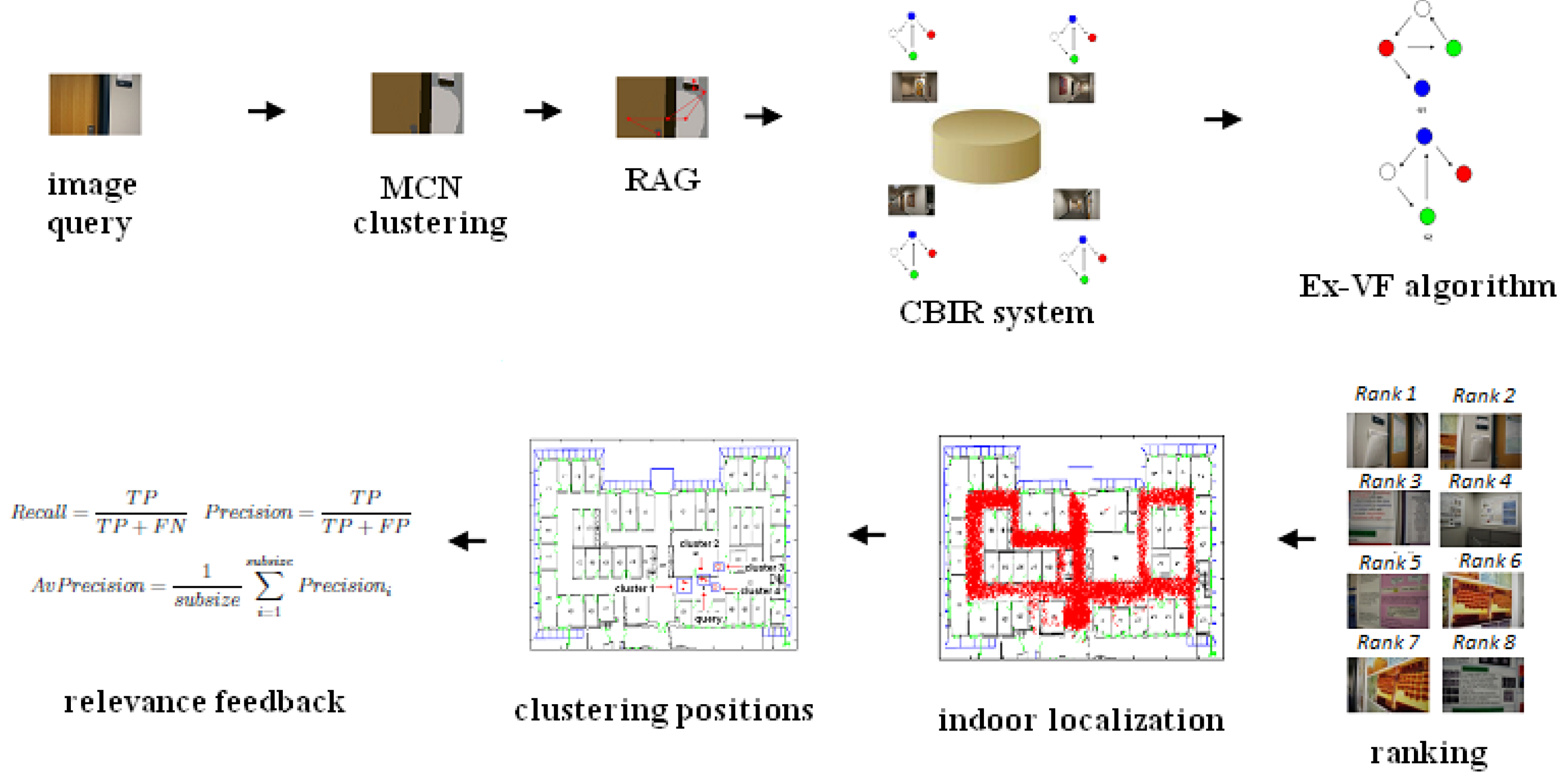
In this context, the main contribution resides in the image features and the mechanism adopted to perform the comparison. Up to now, none of the existing approaches have tackled the relations among features in terms of similarity and spatial homogeneity. Our main contribution consists of introducing an approach based on graph-based representation, according to which regions with their corresponding feature vector and the geometric relationship between these regions are encoded in the form of a graph. The problem of localization is thus formulated as an image retrieval problem between a graph-based representation of the image to be localized and those stored in a database. Each region is represented as a Multicolored Neighborhood (MCN) [9], obtained by extending the representation reported in [9] made for an object to a complex scene. A representation, namely, the Multimodal Neighborhood Signature (MNS), was firstly developed by Matas et al. [10]. However, this signature cannot specify whether there are only two segments or more than two present in the Region Of Interest (ROI). Thus, the neighborhoods having more than two-modal color distributions are not efficiently represented; this problem has been solved by the MCN representation. MCN regions are then linked together by graphs; methods such as the Color Adjacency Graph (CAG) [10], Attributed Relational Graph (ARG) [11], and shock graph [12] are prominent in this approach. The problem, then, is formulated as an approximate graph matching problem. One advantage of graph-based representation is that the geometric relationship can be used to encode certain shape information of the object, and any subgraph matching algorithm can be used to identify a single, as well as multiple objects in query images. We adopt here an extended version of algorithm VFgraph matching [13], which is able to solve the classic problem of graph isomorphism generally. Unlike the version in [13], which operates on simple graph structures, the extended-VF graph matching algorithm works with the purpose of analyzing region features (multicolored neighborhood), corresponding to graph nodes, and at the same time, spatial relationships existing between them. Structural relations prove to be fundamental in order to match images in a context of indoor environment scenes. An overview of our systems is reported in Figure 1.
The paper is organized as follows: Section 2 includes related research in image indoor localization. Section 3, Section 4, Section 5 and Section 6 are dedicated to region representation, attributed graph matching, and complexity analysis. Results and conclusions are respectively reported in Section 7 and Section 8.
2. Related Work
The recent literature reports different approaches to image-based indoor localization. Although not all fully related to feature-based content-based image retrieval, on which mainly our approach resides, we briefly introduce them to better contextualize our approach and, consequently, our contribution.
In [14], the JUDOCAoperator detected junctions in the images. Any junction can be split into a series of two-edge junctions (each two-edge junction forms a triangle). The average intensity is calculated, in gray-scale or color images, for each triangle. Thus, the information is stored in a database, as the output of the JUDOCA [15] operator (location of the junction and the orientations of the edges), in addition to the average color calculated. In the retrieval step, the input image is compared with each one in the database using the features extracted.
The authors in [16] adopted PCA-SIFT [17] features and fast nearest neighbor search based on LSH [18] for image search. Then, the error in the corresponding points was removed by the RANSAC [19] algorithm. Finally, it was necessary to quickly search corresponding image points since the database contained many reference images.
The system proposed in [20] applied a reduction on SIFT features extracted from images. The comparison was performed to measure the feature’s retrieval rate between each image and the entire database. To this end, an image was retrieved if it matched at least five keypoints with the query. This match was considered good if the common content view of two images overlapped.
In [21], the ways to achieve natural landmark-based localization using a vision system for the indoor navigation of an Unmanned Aerial Vehicle (UAV) were discussed. The system first extracted feature points from the image data, taken by a monocular camera, using the SIFT algorithm. Landmark feature points, having distinct descriptor vectors among the feature points, were selected. Then, the position of landmarks was calculated and stored in a map database. Based on the landmark information, the current position of the UAV was retrieved.
In [22], an application for mobile robot navigation was proposed. The system worked on the visual appearance of scenes. For example, scenes, with different locations, that contain repeated visual structures such as corridors, doors, or windows, occur frequently and are recognized as the same. The goal of the proposed method was to recognize the location in the scenes possessing similar structures. The images were described through the salient region, extracted from images using the visual attention model and calculating weights using distinctive features in the salient region. The test phase provided results about single-floor corridor recognition and multi-floor corridor recognition with an accuracy of 78.2% and 71.5%, respectively.
In [23], a new Simultaneous Localization And Mapping (SLAM) algorithm based on the Square Root Unscented Kalman Filter (SRUKF) was described. The logic of the algorithm was based on the square root unscented particle filter for estimating the robot states in every iteration. Afterwards, SRUKF was used to localize the estimated landmarks. Finally, the robot states and landmark information were updated. The algorithm was applied in combined way with the robot motion model and observation model of infrared tag in the simulation. Experimental results showed that the algorithm improved the accuracy and stability of the estimated robot state and landmarks in SLAM.
In [24], the localization problem was addressed by querying a database of omnidirectional images that represented in detail a visual map of the environment. The advantage of omnidirectional consisted, compared to standard perspectives, of capturing in a single frame the entire visual content of a room. This improved the acquisition process of data and favored scalability by significantly decreasing the size of the database. The images were described through an extension of the SIFT algorithm that significantly improved point matching between the two types of images with a positive impact on the recognition based on visual words. The approach was compared with the classical bag-of-words against the recent framework of visual phrases and reported an improvement of localization performance.
In [25], a robust method of self-localization for mobile robots based on a USB camera in order to recognize a landmark in the environment was proposed. The method adopted the Speeded Up Robust Features (SURF) method [26] that is robust to recognize landmark. Then, mobile robot positions were retrieved based on the results of SURF.
In [27], an approach to indoor localization and pose estimation in order to support augmented reality applications on a mobile camera phone was proposed. The system was able to localize the device in an indoor environment and determine its orientation. Furthermore, 3D virtual objects from a database were projected into the image and displayed for the mobile user. Data acquisition was performed off-line and consisted of acquiring images at different locations in the environment. The on-line pose estimation was done by a feature-based matching between the cell phone image and an image selected from the pre-computed database. The algorithm accuracy was evaluated in terms of the reprojection distance of the 3D virtual objects in the cell phone image.
In [28], a mobile device used by the user to help the localization estimation in indoor environments was described. The system was centered on a hybrid method that combined Wi-Fi and object detection to estimate user location in indoor environments. The Wi-Fi localization consisted of a fingerprinting approach using a naive Bayes classifier to analyze the signals of existing networks and give a rougher position estimation. Object detection was accomplished via feature matching between the image database of environment and the image being captured by the camera device in real time.
In [29], the authors presented a probabilistic motion model in which the indoor map was represented in the form of graph. In particular, the motion of the user was followed through the building floor plan. The floor plan was represented as an arrangement of edges and open space polygons connected by nodes.
In [30], the authors provided an indoor localization method to estimate the location of a user. A matching approach between an actual photograph and a rendered BIM (Building Information Modeling) image was adopted. A Convolutional Neural Network (CNN) was used for feature extraction.
In [31], the authors described an approach that recovered the pose of the camera from the 2D points, image positions, and 3D points of the scene model correspondence in order to obtain the initial location and eliminate the accumulative error when an image was successfully registered. However, the image was not always registered since the traditional 2D-to-3D matching rejected different correct correspondences when the view became large. A robust image registration strategy was adopted to recover initially unregistered images by integrating the 3D-to-2D search.
In [32], a large-scale visual localization method for indoor environments was proposed. The authors worked based on three steps: recovery of candidate poses, pose estimation using dense matching different from local features, and pose verification by virtual view synthesis to address the changes in the viewpoint, scene layout, and occluders.
In [33], a framework for performing fine localization and less latency with more a priori information was proposed. The system worked in off-line mode and used SURF to represent the image database, and on-line mode position and direction angle estimation by the homography matrix and learning line was performed.
In [34], the authors combined wireless signals and images to improve the positioning performance. The framework adopted Local Binary Patterns (LBP) to represent images. Localization worked through two steps: first, obtaining a coarse-grained estimation based on wireless signals and, second, to determine the correspondences between two-dimensional pixels and three-dimensional points based on images collected by the smartphone.
According to our approach, the problem of localization is formulated as an image retrieval problem between a graph-based representation of the image to be localized and that stored in a database. In the following sections, details about the region representation and graph-matching-based image retrieval will be given.
3. Region Representation
Color information and pattern appearance are included in the image representation. A way of preserving the position of adjacent segments is to store their color vector representation as units. These units, linked together, cover all segments of adjacent pixels in the ROI. The region is called the MultiColored Neighborhood (MCN) [9].
To keep track of structural information, for each MCN, the value of color found from the centroids of clusters was stored as a unit. The colors represented by the centroids of clusters were formed through the vectors present in MCN. This unit of cluster centroids contained the average color value corresponding to the different segments of the MCN. Ultimately, the scene was represented by the Multicolored Region Descriptor (M-CORD) in terms of the distinct sets of units of the cluster centers of the constituent MCNs. Suppose we have N distinct MCNs. The region contains N units of cluster centroids, and each unit represents a single centroid of an MCN. This descriptor contains the information about each MCN. As a consequence, if there is a unit of clusters present in the descriptor, then there is a set of pixels that cover segments in an image. This greatly improves the discriminating power of the recognition system when the same, but differently-aligned, colors are present in two objects.
Since the distribution of the color of each MCN is multimodal, a clustering technique can be adopted to find the number of colors in a region and construct the M-CORD. The clustering algorithm is applied to overlapping windows extracted from the image.
After having found an MCN, this is matched with all of the previously-considered MCNs and is included in the descriptor if it is significantly different from all the previously-considered MCNs.
The input parameters of the clustering algorithm used to obtain MCNs are:
. , is the set of color vectors. The difference between and is given by , where r is the dissimilarity parameter, and the dissimilarity between sets V is computed according to the Hausdorff distance, which measures the degree of mismatch between two sets. The advantage of the use of this distance, in our case, is that it was not applied to a single-color vector irrespective of all other color vectors. This distance provides more stability and accuracy in calculating the proximity between two sets (color vectors). is the parameter to check the validity of clusters. It needs distances and comparisons to find a region with a uniform color, because in each region, all color vectors are within a disk of radius r centered on .
For surrounding pixels that have more than one cluster, distance computations are necessary. In any case, the number of comparisons increases with the number of clusters.
4. Region Adjacency Graph
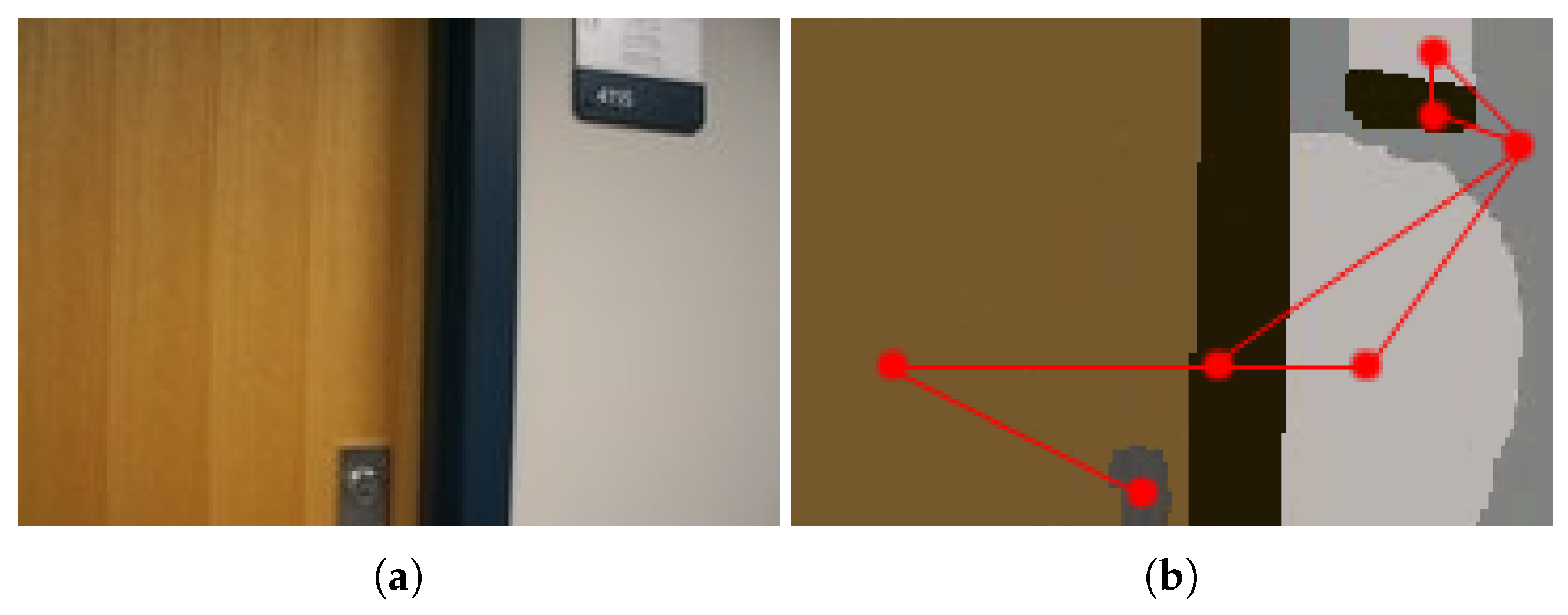
The Region Adjacency Graph (RAG) [35] was used to build the scene representation. The RAG was constructed as follows. Let us consider the clustering result, which has the purpose of recognizing pixels that can be considered as belonging to the same class. After that, each pixel set, region R, can be considered as an elementary component of the image. Finally, the RAG was built based on the spatial relations between regions. Two regions were defined to be adjacent if they shared the same boundary. In the graph, a node represents a region, and a link represents adjacency between two nodes. Each node is associated with the relevant properties of the region (color), i.e., the M-CORD. An example of RAG, based on M-CORD, is reported in Figure 2b.
Formally, a RAG, , is an undirected graph such that:
N is the set of nodes in the graph, where a node corresponds to a region and:
if the corresponding regions and are located adjacent in the image (connected). A neighborhood system can be defined on G, denoted by:
where , with , is the set of all the nodes in N that are neighbors of , such that:
is not connected with itself (loop), and if:
is connected with , then:
is connected with . Given two graphs, representing scenes, it is possible to compare them using a graph matching algorithm; we adopt the algorithm described in [13], properly extended to take into account the M-CORD attached to each node.
5. Extended VF Graph Matching
A matching process between two graphs and is the determination of a mapping M that associates nodes of the graph with nodes of the graph , and vice versa. Different types of constraints may be imposed on M, and consequently, different types of matching can be obtained: morphism [36], isomorphism [37], and isomorphism of a sub-graph [38]. Generally, the mapping M is expressed as a set of ordered pairs (with and ), each representing the matching of a node n of with a node m of . According to the extended VF algorithm, the graph-matching process can be efficiently described using a State Space Representation (SSR), where for each state process s, a partial mapping is a subset of M, containing some components of M. A partial mapping refers to two subgraphs of and , and and , obtained with a selection of nodes of and included in and the connections among them. Moreover, and can be defined as the projection of in and the projection of in , while the sets of the branches of and are identified by and . can be defined as the set of all the possible pair candidates to be added to the current state considering first the sets of the nodes directly connected to and . Additionally, the out-terminal set can be defined as the set of nodes of not in , but with successors of a node in , and the in-terminal set can be defined as the set of nodes that are not in , but with predecessors of a node in . In the same way, and can be defined. In the SSR, a transition between two states corresponds to the adding of a new pair to nodes that form the mapping. The goal is to reduce the number of paths to be explored during the search (brute force approach), for each state from the route to the target. It requires that the corresponding partial solution checks certain conditions of consistency, based on the desired mapping. For example, to have an isomorphism, it is necessary that the solutions be partial isomorphisms between the corresponding sub-graphs. If the addition of a node pair produces a solution that does not match the conditions of consistency, then the exploration of this path can be avoided (because it is certain that it will not lead to a state goal). The logic is to introduce criteria for prediction if a state s has no successor after a certain number of steps. It is clear that the criteria (feasibility rules) would find (quickly) the conditions that lead to inconsistency. In particular, given a pair to be included in state s, to obtain a state , a feasibility rule allows determining all inconsistent states reachable from . Therefore, states that do not match the feasibility rules can be discarded for further expansions. Between all combinations of SSR allowed, only a small part conforms to the type of morphism sought, and there is no way that prevents the achievement of the complete solution. and related to are isomorphic if the condition of consistency is verified for graph isomorphism or subgraph isomorphism search.
6. Complexity Analysis
In this section, we analyze the computational complexity of the image feature extraction algorithm and the graph-matching algorithm.
The Multicolored Neighborhood (MCN) clustering, used to extract M-CORD from the image, is designed to perform the union of k clusters, , as , which compose the output image, where is the set of color vectors. The number of comparisons required to partition all vectors in V in 1 clusters is equal to:
where denotes the number of elements in . Additionally, at most n vector additions and k divisions are needed for the computation of centroids. In any case, the number of comparisons increases with the number of clusters. Then, the computational time complexity is . The execution time and success is strongly dependent on the number of clusters k that will compose the number of components of the output image.
The computational complexity of the graph matching algorithm can be computed in a different way. The extended-VF algorithm works based on SSR. In SSR, the next state is obtained by adding a pair to the previous state, and the cost for this operation can be decomposed into three terms:
- the cost needed to verify if the new state satisfies the feasibility rules;
- the cost needed to calculate the sets associated with the new state;
- the cost needed to generate the sets of the pair candidates for inclusion in the current state.
The first two terms have a cost proportional to the number of branches having n or m as an endpoint. The operations needed for each branch can be performed in constant time proportional to the number of branches. If we denote this quantity with b, the cost for the first two terms will be .
The third term requires a number of operations that is at least proportional to the number of nodes of the two graphs. In order to find all the pair candidates for the inclusion in the current state, it is necessary to examine the node of with the smallest label and all the nodes of belonging to (spending a time proportional to the number of nodes in and ). If we suppose that the two graphs have the same number N of the nodes, the total cost for this term will be . Meanwhile, if the two graphs have a number of different nodes, the term will be . In the worst case, in each state, the predicate will not be able to avoid the visit of any successors, and the algorithm will have to explore all the states before reaching a solution. This situation may occur if the graphs exhibit strong symmetries, for example if they are almost completely connected and the algorithm takes a long time to reach the final solution. Therefore, in order to improve this aspect, it is important to reduce the number of clusters k for image representation, especially when including little information, which affects the matching phase.
7. Image Search for Indoor Localization: Experimental Results
For testing, we adopted a dataset of images with associated location information [1]. Starting from the input image, the framework tried to find similar images in the database. Using the pre-annotated location information, an estimation of input image location can be performed.
The dataset was composed of about 8.8 thousand images in an indoor environment, accompanied by a floor plan map. A location label was associated with each image. The images were located with two types of coordinates: actual world coordinates and floor plan coordinates. The ratio between them was 0.0835.
The goal was to locate an input image within the indoor environment based on associated spatial coordinates. Based on similar images returned by the image retrieval system, the position of the query image can be found.
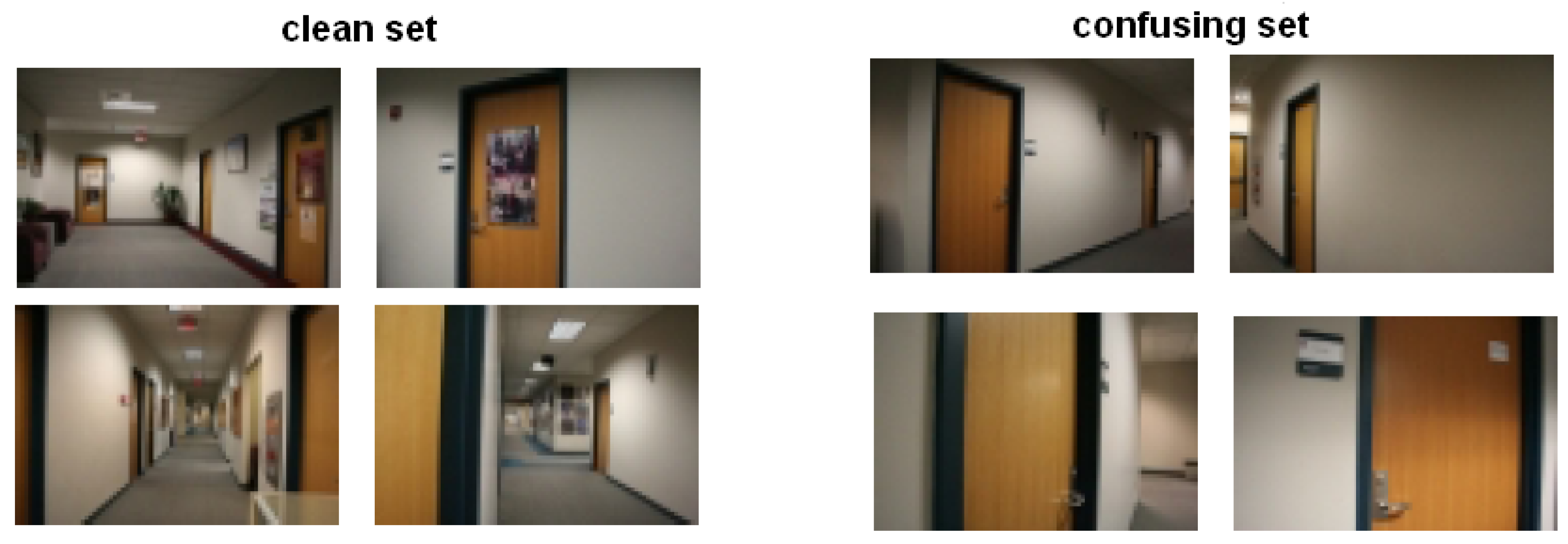
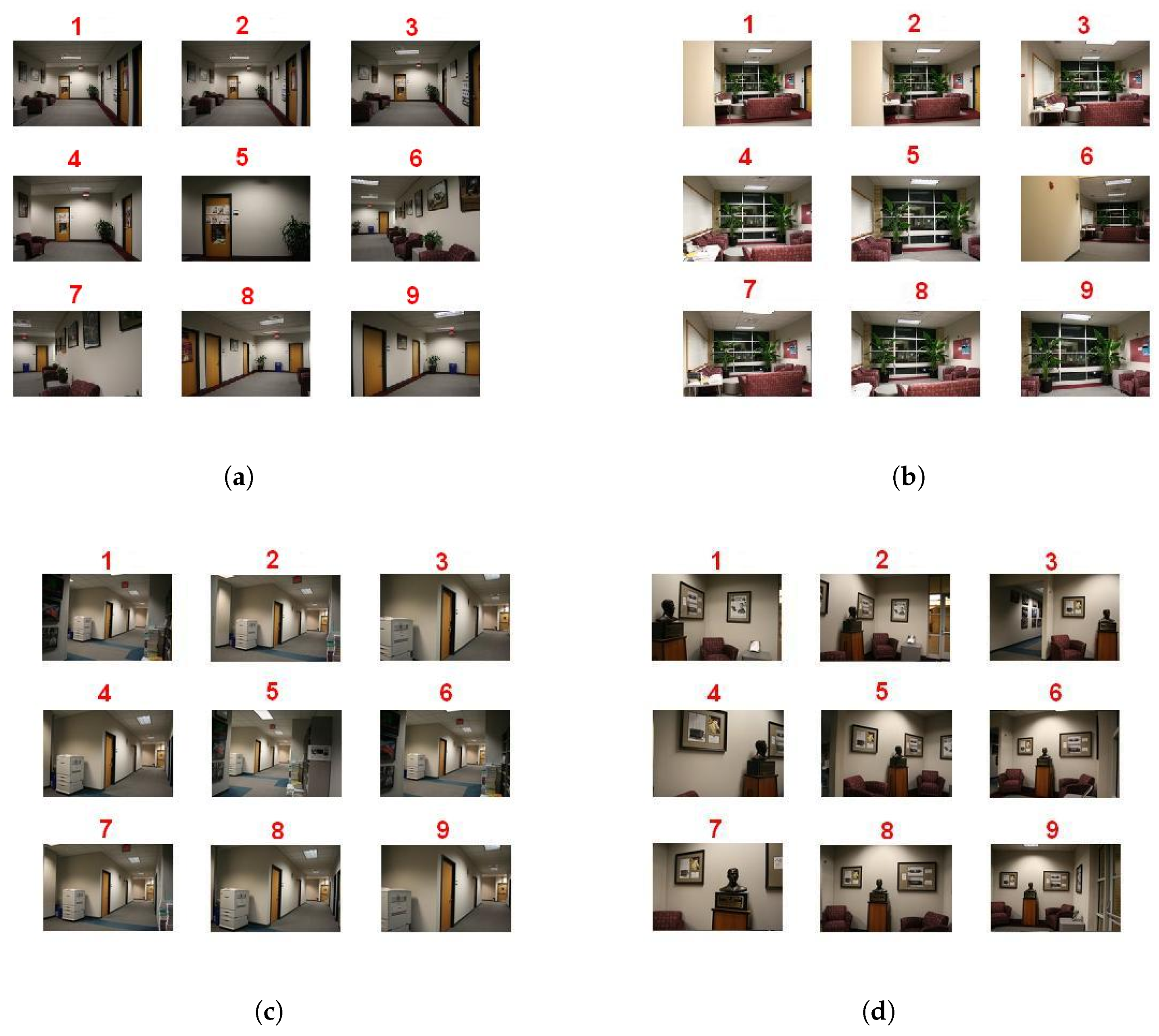
For testing, two types of images were chosen. One set had rich and distinctive visual structures, named the “clean set”. A different set contained images with the details of the scene such as windows or doors. This set was called the “confusing set”. In both sets were included 80 images. Some examples of the “clean set” and “confusing set” are reported in Figure 3.
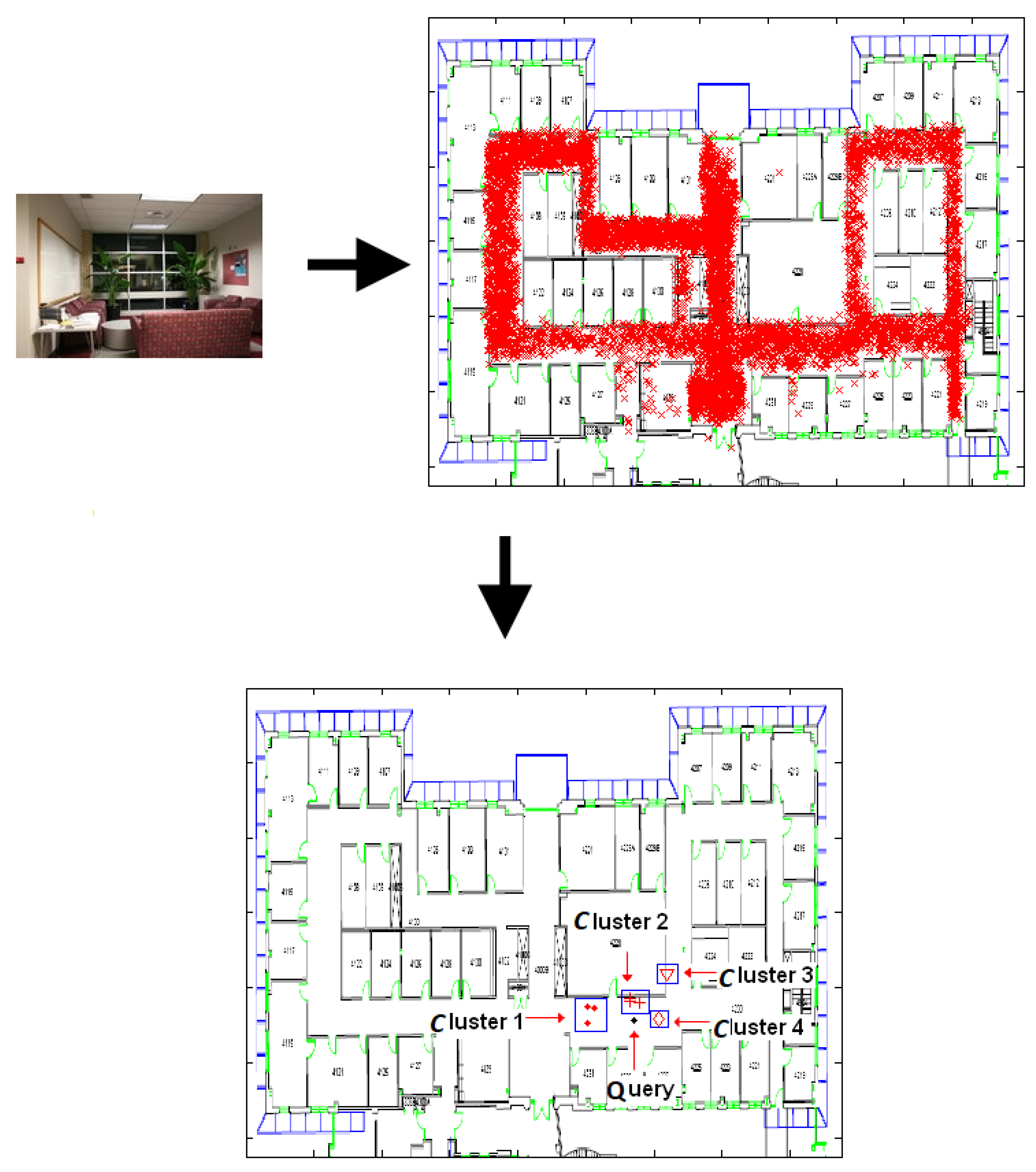
Recall-precision was adopted to measure the performance. Given an image query, eight top-ranked images were shown. A potential localization was performed if a cluster existed, denoted by R, of pre-recorded images captured less than three meters away from each other in the retrieval set (based on spatial coordinates). If more than one cluster existed, the system considered the larger and higher ranked set. An example is show in Figure 4.
Figure 4 shows how the prediction, for an input image, was done for user localization. The position of the first eight images from the ranking was drawn in the reference layout of the environment where they were taken. It should be remarked that images belonging to the same cluster were labeled with the same shape. In addition, the query image was identified with a different color from the color assigned to the retrieved images. In this case “Cluster 2” was chosen as the set R, because it contained a larger number of images and had a better position in the ranking. denotes the size of set R. Using a threshold, identified by , which regulates the minimum size of R, the precision of localization can be changed for each prediction. At this point, there are three different cases:
- : the size of satisfies the condition of the minimum size of the cluster, and all images contained in R are used for prediction;
- : the localization fails;
- : the result of the previous step of clustering is not considered, and information associated with the first image in the ranking is adopted for prediction.
Having chosen the cluster R, a step of relevance feedback was started. The values of , , and were computed as follows:
- : the query image with a correspondence in the database can be considered as a false negative;
- : false positives can be defined as the images, having a correspondence with the query image, in R with a minimum position distance of more than three meters;
- : true positives can be defined as the images, having a correspondence with the query image, in R with a minimum position distance of less than three meters;
From these three values, recall, precision, and average precision measures can be calculated as follows, remarking that is relative to the query of the subset of dimension and the number of queries used to calculate the is equal to :
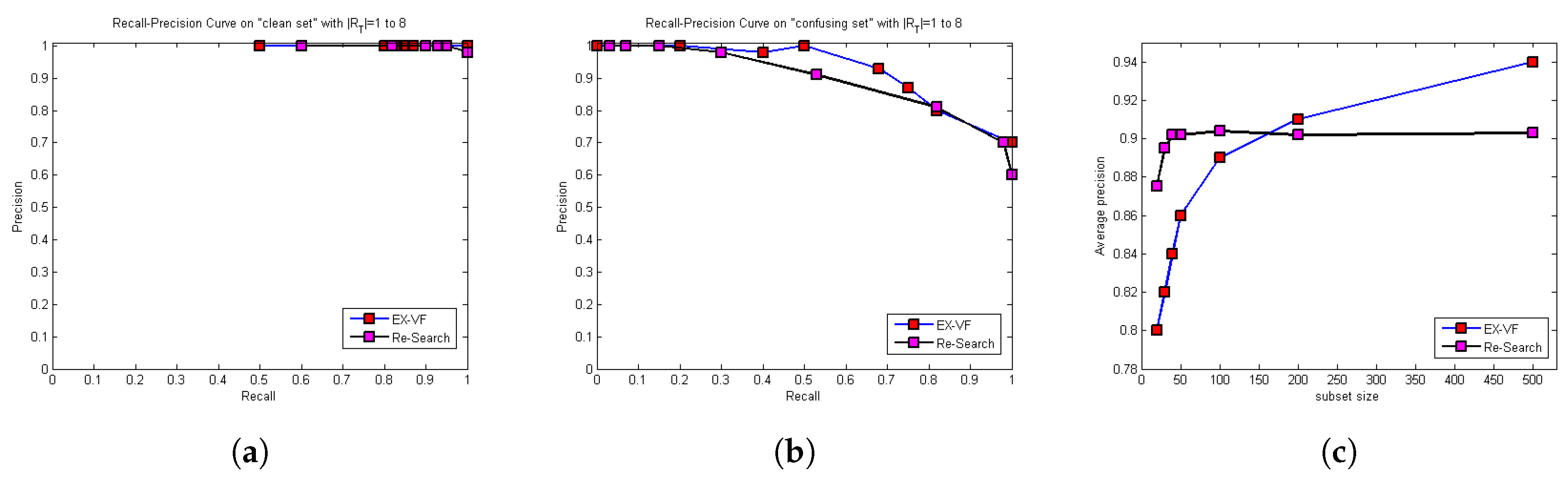
Figure 5a,b show the recall-precision curves using the algorithm on both testing sets. The measures were computed for (integer) values for in the set . The feedback on the “clean set” provided improved performance and showed that the system could be adopted for the indoor localization scenario. For the “confusing” set, the test was very interesting because it is a common situation in which the user can be found. Finally, Figure 5c shows the performance when the subset size changed. This further test concerned an important aspect of our system. The goal was to analyze the behavior of the proposed technique with a growing amount of data. In fact, with increasing images in the test set, performance may decrease due to the large number of false positives. Our system, even if execution times slowed down, improved performance, because it was able to filter out false positives and include true positives. This behavior did not occur for the Re-Search technique.
Figure 6 shows examples of localization. The goal was to find the same scene of the query image and then locate the user within the indoor environment. In Figure 6a–d, Image 1 is the query. In all results, the query image was very similar compared to the images retrieved from the system.
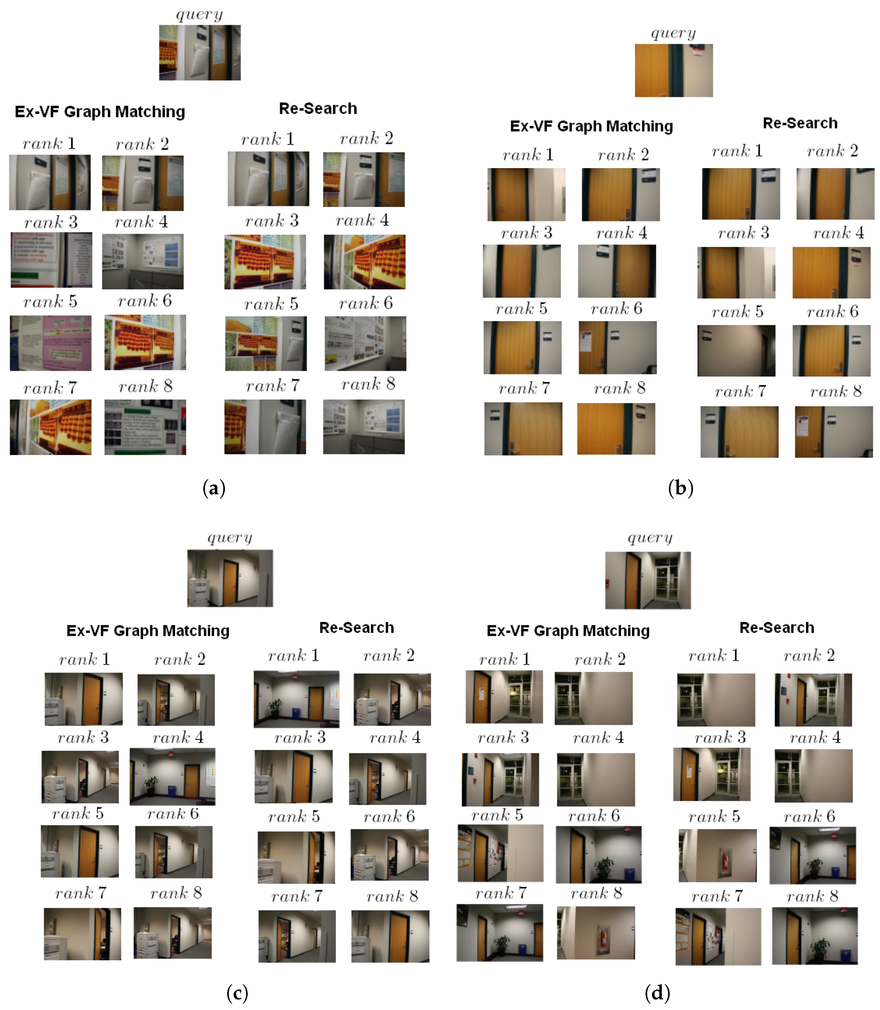
Figure 7 shows more qualitative comparisons. As can be seen, the proposed approach retrieved relevant images, in terms of the visualizationof the scene, related to query images. In this way, the prediction of localization produced a result very close to the real position of the user. Comparisons were also made with the technique in [1], named Re-Search. The Re-Search technique approaches the image matching problem in two steps. Firstly, most images matched to a query image are retrieved. The Harris-Affine (HARAFF) region detector [39] and SIFT [3] are adopted. A vocabulary tree is built for indexing and searching the database.
The result was a small number (top 50 retrievals) of similar candidates for the query image. Secondly, the TF-IDF approach inspired by the textual retrieval field was adopted for visual words representing the images.
The comparison with the technique Re-Search proved the effectiveness of the algorithm extended-VF graph matching in a localization scenario. In order to measure the quality of results obtained using both techniques, rankings in Figure 7 are analyzed. Images ranked on the top were more similar with respect to the query image in both cases. This aspect may be justified by the phase of feature extraction (MCN clustering), which was able to capture parts in the scene, e.g., the door in the second case of Figure 7b, which were represented in all the images (single node in the graph) and, thus, detected by the algorithm.
Further tests were conducted, in order to prove the effectiveness of our approach, using the same dataset and criteria for the localization procedure. The first experiment consisted of a comparison with different features extracted from the image. Our approach was based on MCN clustering with the purpose of representative colors’ detection. In a different way, the K-means algorithm was applied to find cluster centers from several regions in the image. Color features and, consequently, the graph structure, for image representation, were differently built. In both cases, for the matching phase, we adopted the algorithm extended-VF graph matching. Furthermore, for performance evaluation, an additional relevance feedback measure was introduced: .
is defined as, for a set of queries, the mean of the average precision scores for each query. Q is the number of queries. Table 1 contains the results achieved. It can be noted that MCN clustering provided better performance than K-means. Indeed, regions with a uniform color, corresponding to objects in the scene, were extracted. These objects, represented with nodes in the graph structure, were easily detected by the graph-matching algorithm.
The second additional experiment concerned a comparison with two other approaches working in the same localization scenario. The first approach selected was a baseline algorithm named Nistér and Stewénius [40] that uses a hierarchical K-means algorithm for vocabulary generation and a multi-level scoring strategy. The second approach was an image indexing and matching algorithm that performs a distinctive selection of high-dimensional features [41]. A bag-of-words algorithm combined the feature distinctiveness in visual vocabulary generation. Table 1 includes results for the comparison of the algorithms. For the “clean set”, the best performance was provided for the D_BOW algorithm and our approach. While, for the confusing set, our approach outperformed the algorithms used for comparison.
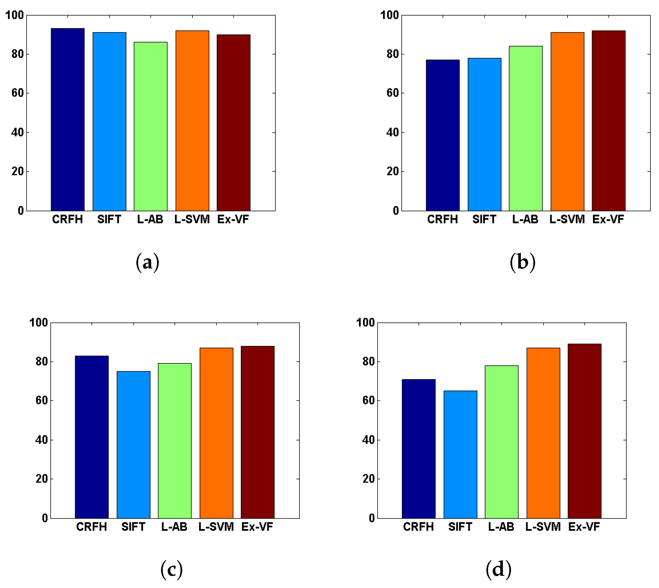
Finally, further tests were conducted using a different indoor environment database: KTH-IDOL2 [2]. The database contains 24 image sequences, with about 800 images for each sequence. The images were acquired in different real-world scenarios (one-person office, two-person office, corridor, kitchen, and printer area), over a span of six months and under different illumination and weather conditions (cloudy weather, sunny weather, and night). Consequently, different visual variations in an indoor environment were captured in the sequences. In this context, four image sets were created. The first set contained different combinations of training and test data acquired closely in time and under similar illumination conditions. On this set were performed 12 experiments. On the second set of experiments were used 24 pairs of sequences captured still at relatively close times, but under different illumination conditions. On third set, consisting of 12 experiments, tests were related to data acquired six months later and under similar illumination conditions. On the last set, both types of variations were combined, and experiments were performed on 24 pairs of subsets, obtained six months from each other and under different illumination settings. The measure of performance used was the percentage of correct images classified for each room. Subsequently, the average was calculated with equal weights independent of the number of images related to each room. Performance were evaluated through a comparison with four types of models: SVM based on visual features, CRFH [42] and SIFT [3], and AdaBoost [43] and SVM trained on Laser range features (L-AB and L-SVM) [44]. The results of the experiments are presented in Figure 8a–d. On the first set, Figure 8a, according to the expectations, CRFH and SIFT suffered from changes in illumination, as our approach, differently from the geometric laser-based features. In other cases, Figure 8b–d, our approach produced different performances and outperformed the comparison techniques with percentages of 92.0%, 88.0%, and 89.0%.
In Figure 9, some additional tests on the KTH-IDOL2 database are shown. In both cases, Image 1 was the query, and retrieved images included its own scene.
To solve the problem of illumination variations, different representations of the same scene were captured both client-side (image queries) and server-side (image database). Furthermore, in this way, all details of the scene were correctly captured. This certainly enhanced the image database and also improved, of course, the results of user localization.
8. Conclusions
A novel way to capture visual information in an indoor environment was reported. The approach was graph-based and mainly resided on a very peculiar algorithm of feature extraction and scene representation, MCN, which was shown as a valid alternative to classical techniques such as color, shape, and texture. The robustness and effectiveness of the image matching algorithm were demonstrated while detecting, in an indoor environment, confusing and self-repetitive patterns. The feedback obtained from testing using the technique of graph matching was positive, specifically with the increasing of images in the database, and sometimes even higher in terms of retrieved relevant images. The main disadvantages of the proposed technique concerned the image representation in situations with little structure and confused scenes in which the phase of clustering reports many clusters with little information, resulting in a high number of nodes of the graph. Clearly, a satisfactory result could not be achieved during the matching phase, and consequently, the localization phase failed.
The first future development concerns an on-line version of the Ex-VF algorithm for real-time performance. In this context, statistical models can be learned in order to tune the algorithm settings and to improve the performance. Another important issue concerns the correspondence between real map position and database images. A solution concerns the application of structure from motion methods to obtain the camera position and ground truth information. Finally, a further goal is the use different features in the creation of a graph structure in order to improve localization performance.
In conclusion, it appears clear that the reported tool can be used as an interesting alternative, in restricted scenarios, to other positioning systems to locate users in indoor environments.
Funding
This research received no external funding.
Acknowledgments
This work is dedicated to Alfredo Petrosino. With him, I took my first steps in the field of computer science. During these years spent together, I learned the firmness of achieving the goals and the love and passion for the work. I will be forever grateful. Thank you my great master.
Conflicts of Interest
The author declares no conflict of interest.
References
- Kang, H.; Efros, A.A.; Hebert, M.; Kanade, T. Image matching in large scale indoor environment. In Proceedings of the 2009 IEEE Computer Society Conference on Computer Vision and Pattern Recognition Workshops, Miami, FL, USA, 20–25 June 2009; pp. 33–40. [Google Scholar]
- Pronobis, A.; Mozos, O.M.; Caputo, B. SVM-based discriminative accumulation scheme for place recognition. In Proceedings of the 2008 IEEE International Conference on Robotics and Automation, Pasadena, CA, USA, 19–23 May 2008; pp. 522–529. [Google Scholar]
- Lowe, D.G. Distinctive image features from scale-invariant keypoints. Int. J. Comput. Vis. 2004, 60, 91–110. [Google Scholar] [CrossRef]
- Csurka, G.; Dance, C.; Fan, L.; Willamowski, J.; Bray, C. Visual categorization with bags of keypoints. In Proceedings of the ECCV Workshop on Statistical Learning in Computer Vision, Prague, Czech Republic, 11–14 May 2004. [Google Scholar]
- Neira, J.; Tardós, J.D. Data association in stochastic mapping using the joint compatibility test. IEEE Trans. Robot. Autom. 2001, 17, 890–897. [Google Scholar] [CrossRef]
- Filliat, D. A visual bag of words method for interactive qualitative localization and mapping. In Proceedings of the 2007 IEEE International Conference on Robotics and Automation, Roma, Italy, 10–14 April 2007; pp. 3921–3926. [Google Scholar]
- Richard, A.; Gall, J. A bag-of-words equivalent recurrent neural network for action recognition. Comput. Vis. Image Underst. 2017, 156, 79–91. [Google Scholar] [CrossRef] [Green Version]
- Passalis, N.; Tefas, A. Learning bag-of-features pooling for deep convolutional neural networks. In Proceedings of the IEEE International Conference on Computer Vision, Venice, Italy, 22–29 October 2017; pp. 5755–5763. [Google Scholar]
- Naik, S.K.; Murthy, C. Distinct multicolored region descriptors for object recognition. IEEE Trans. Pattern Anal. Mach. Intell. 2007, 29, 1291–1296. [Google Scholar] [CrossRef] [PubMed]
- Matas, J.; Koubaroulis, D.; Kittler, J. The multimodal neighborhood signature for modeling object color appearance and applications in object recognition and image retrieval. Comput. Vis. Image Underst. 2002, 88, 1–23. [Google Scholar] [CrossRef]
- Ahmadyfard, A.; Kittler, J. Using relaxation technique for region-based object recognition. Image Vis. Comput. 2002, 20, 769–781. [Google Scholar] [CrossRef]
- Siddiqi, K.; Kimia, B.B. A shock grammar for recognition. In Proceedings of the CVPR IEEE Computer Society Conference on Computer Vision and Pattern Recognition, San Francisco, CA, USA, 18–20 June 1996; pp. 507–513. [Google Scholar]
- Cordella, L.P.; Foggia, P.; Sansone, C.; Vento, M. A (sub) graph isomorphism algorithm for matching large graphs. IEEE Trans. Pattern Anal. Mach. Intell. 2004, 26, 1367–1372. [Google Scholar] [CrossRef] [PubMed]
- Elias, R.; Elnahas, A. An accurate indoor localization technique using image matching. In Proceedings of the 3rd IET International Conference on Intelligent Environments, Ulm, Germany, 24–25 September 2007. [Google Scholar]
- Laganiere, R.; Elias, R. The detection of junction features in images. In Proceedings of the 2004 IEEE International Conference on Acoustics, Speech, and Signal Processing, Montreal, QB, Canada, 17–21 May 2004. [Google Scholar]
- Kawaji, H.; Hatada, K.; Yamasaki, T.; Aizawa, K. Image-based indoor positioning system: Fast image matching using omnidirectional panoramic images. In Proceedings of the 1st ACM international workshop on Multimodal pervasive video analysis, Firenze, Italy, 25–29 October 2010; pp. 1–4. [Google Scholar]
- Ke, Y.; Sukthankar, R. PCA-SIFT: A more distinctive representation for local image descriptors. In Proceedings of the 2004 IEEE Computer Society Conference on Computer Vision and Pattern Recognition, Washington, DC, USA, 27 June–2 July 2004; pp. 506–513. [Google Scholar]
- Datar, M.; Immorlica, N.; Indyk, P.; Mirrokni, V.S. Locality-sensitive hashing scheme based on p-stable distributions. In Proceedings of the Twentieth Annual Symposium on Computational Geometry, Brooklyn, NY, USA, 8–11 June 2004; pp. 253–262. [Google Scholar]
- Fischler, M.A.; Bolles, R.C. Random sample consensus: a paradigm for model fitting with applications to image analysis and automated cartography. Commun. ACM 1981, 24, 381–395. [Google Scholar] [CrossRef]
- Ledwich, L.; Williams, S. Reduced SIFT features for image retrieval and indoor localisation. In Proceedings of the Australian Conference on Robotics and Automation, Canberra, Australia, 6–8 December 2004; Volume 322, p. 3. [Google Scholar]
- Lee, J.O.; Kang, T.; Lee, K.H.; Im, S.K.; Park, J. Vision-based indoor localization for unmanned aerial vehicles. J. Aerospace Eng. 2010, 24, 373–377. [Google Scholar] [CrossRef]
- Yoon, K.Y.; Choi, S.W.; Lee, C.H. An approach for localization around indoor corridors based on visual attention model. J. Inst. Control Robot. Syst. 2011, 17, 93–101. [Google Scholar] [CrossRef]
- Zhao, L.; Sun, L.; Li, R.; GE, L. On an improved SLAM algorithm in indoor environment. Robot 2009, 31, 438–444. [Google Scholar]
- Lourenço, M.; Pedro, V.; Barreto, J.P. Localization in indoor environments by querying omnidirectional visual maps using perspective images. In Proceedings of the 2012 IEEE International Conference on Robotics and Automation, Saint Paul, MN, USA, 14–18 May 2012; pp. 2189–2195. [Google Scholar]
- Muramatsu, S.; Chugo, D.; Jia, S.; Takase, K. Localization for indoor service robot by using local-features of image. In Proceedings of the 2009 ICCAS-SICE, Fukuoka, Japan, 18–21 August 2009; pp. 3251–3254. [Google Scholar]
- Bay, H.; Tuytelaars, T.; Van Gool, L. Surf: Speeded up robust features. In Proceedings of the ECCV, Graz, Austria, 7–13 May 2006; pp. 404–417. [Google Scholar]
- Paucher, R.; Turk, M. Location-based augmented reality on mobile phones. In Proceedings of the CVPR 2010, San Francisco, CA, USA, 13–18 June 2010; pp. 9–16. [Google Scholar]
- Morimitsu, H.; Pimentel, R.B.; Hashimoto, M.; Cesar, R.M.; Hirata, R. Wi-Fi and keygraphs for localization with cell phones. In Proceedings of the ICCV Workshops, Barcelona, Spain, 6–13 November 2011; pp. 92–99. [Google Scholar]
- Koivisto, M.; Nurminen, H.; Ali-Loytty, S.; Piche, R. Graph-based map matching for indoor positioning. In Proceedings of the ICICS, Beijing, China, 9–11 December 2015; pp. 1–5. [Google Scholar]
- Ha, I.; Kim, H.; Park, S.; Kim, H. Image-based Indoor Localization using BIM and Features of CNN. In Proceedings of the ISARC, Berlin, Germany, 20–25 July 2018; Volume 35, pp. 1–4. [Google Scholar]
- Zhou, Y.; Zheng, X.; Chen, R.; Xiong, H.; Guo, S. Image-based localization aided indoor pedestrian trajectory estimation using smartphones. Sensors 2018, 18, 258. [Google Scholar] [CrossRef] [PubMed]
- Taira, H.; Okutomi, M.; Sattler, T.; Cimpoi, M.; Pollefeys, M.; Sivic, J.; Pajdla, T.; Torii, A. InLoc: Indoor visual localization with dense matching and view synthesis. In Proceedings of the CVPR, Salt Lake City, 18–22 June 2018; pp. 7199–7209. [Google Scholar]
- Guan, K.; Ma, L.; Tan, X.; Guo, S. Vision-based indoor localization approach based on SURF and landmark. In Proceedings of the IWCMC, Paphos, Cyprus, 5–9 September 2016; pp. 655–659. [Google Scholar]
- Jiao, J.; Li, F.; Tang, W.; Deng, Z.; Cao, J. A hybrid fusion of wireless signals and RGB image for indoor positioning. Int. J. Distrib. Sens. Netw. 2018, 14, 1550147718757664. [Google Scholar] [CrossRef]
- Trémeau, A.; Colantoni, P. Regions adjacency graph applied to color image segmentation. IEEE Trans. Image Process. 2000, 9, 735–744. [Google Scholar] [CrossRef] [PubMed]
- Bandler, W.; Kohout, L.J. On the genearl theory of relational morphisms. Int. J. Gen. Syst. 1986, 13, 47–66. [Google Scholar] [CrossRef]
- Bunke, H.; Allermann, G. Inexact graph matching for structural pattern recognition. Pattern Recognit. Lett. 1983, 1, 245–253. [Google Scholar] [CrossRef]
- Ullmann, J.R. An algorithm for subgraph isomorphism. JACM 1976, 23, 31–42. [Google Scholar] [CrossRef]
- Mikolajczyk, K.; Schmid, C. Scale & affine invariant interest point detectors. Int. J. Comput. Vis. 2004, 60, 63–86. [Google Scholar]
- Nister, D.; Stewenius, H. Scalable recognition with a vocabulary tree. In Proceedings of the CVPR, New York, NY, USA, 17–22 June 2006; Volume 2, pp. 2161–2168. [Google Scholar]
- Kang, H.; Hebert, M.; Kanade, T. Image matching with distinctive visual vocabulary. In Proceedings of the WACV, Kona, HI, USA, 5–7 January 2011; pp. 402–409. [Google Scholar]
- Linde, O.; Lindeberg, T. Object recognition using composed receptive field histograms of higher dimensionality. In Proceedings of the ICPR, Cambridge, UK, 23–26 August 2004; Volume 2, pp. 1–6. [Google Scholar]
- Freund, Y.; Schapire, R.E. A decision-theoretic generalization of on-line learning and an application to boosting. J. Comput. Syst. Sci. 1997, 55, 119–139. [Google Scholar] [CrossRef]
- Mozos, O.M.; Stachniss, C.; Burgard, W. Supervised learning of places from range data using adaboost. In Proceedings of the ICRA, Barcelona, Spain, 18–22 April 2005; pp. 1730–1735. [Google Scholar]
Figure 1.
Application overview. Given an input image, captured by a user located in an indoor environment, a set of images pre-captured in the same environment is retrieved through the extended-VFmatching algorithm. The location of the user is determined by labels attached to matched images. Finally, the relevance feedback phase calculates the accuracy of the localization prediction. MCN, Multicolored Neighborhood; RAG, Region Adjacency Graph; CBIR, Content-Based Image Retrieval.

Figure 2.
Graph representation: (a) the original image of the indoor environment; (b) RAG based on Multicolored Region Descriptor (M-CORD).
Figure 2.
Graph representation: (a) the original image of the indoor environment; (b) RAG based on Multicolored Region Descriptor (M-CORD).

Figure 3.
Some examples of the “clean set” and “confusing set”.

Figure 4.
The result is the top eight retrieved and clustered images.

Figure 5.
Experimental results for Ex-VF and Re-Search. The integer value used for parameter , minimum size of R, was in the range . (a) The recall-precision curve on the “clean set”. In this case, the performances between approaches were comparable. A slight improvement by our technique can be seen for the value of equal to eight, which produced values of recall-precision equal to one. (b) The recall-precision curve on the “confusing set”. A substantial improvement was obtained for Ex-VF algorithm with a better trend than Re-Search. (c) The effect of changing the subset size (the subset sizes used were 20, 30, 40, 50, 100, 200, and 500 images). In this context, the goal was to analyze the behavior with a growing amount of data. As can be seen, the Ex-VF algorithm outperformed Re-Search, even if the execution times slowed down, because it was able to filter out false positives and include true positives.

Figure 6.
An example illustrating the robustness of the extended-VF graph matching. In the four blocks displayed, images located at the top of the ranking, labeled with 1, are the queries; in other words, images captured by the user, placed in an indoor environment, looking for location information. The remaining are images of ranking. As can seen, the images retrieved were very similar, in terms of the structure of scene, to each query. Indeed, the tests showed that the graph structure captured the scene structural information represented by the colors, extracted using the MCN clustering, and the arrangement of the different elements such as doors, windows, etc., through the application of the region adjacency graph. Finally, the algorithm Ex-VF selected all the images with the same structural representation. Consequently, localization occurred in an effective way. Results in (a), (b), (c) figures concern “clean set” while in (d) figure concerns “confusing set”.

Figure 7.
Some qualitative analysis of the image matching results of Re-Search and extended-VF graph matching. Results in (c), (d) figures concern “clean set” while in (a), (b) figure concern “confusing set”.
Figure 7.
Some qualitative analysis of the image matching results of Re-Search and extended-VF graph matching. Results in (c), (d) figures concern “clean set” while in (a), (b) figure concern “confusing set”.

Figure 8.
Quantitative comparison of Ex-VF with SVM based on visual features, CRFH [42] and SIFT [3], and AdaBoost [43] and SVM trained on Laser range features (L-AB and L-SVM) [44]. (a) Stable illumination conditions, close in time. (b) Varying illumination conditions, close in time. (c) Stable illumination conditions, distant in time. (d) Varying illumination conditions, distant in time.

Figure 9.
Two examples illustrating a test performed on the KTH-IDOL2 database. In this case as well, the Ex-VF algorithm selected all the images similar to the query (top left). Both example, (a,b) represent scenes in which the image contains elements that compose a visual structure.
Figure 9.
Two examples illustrating a test performed on the KTH-IDOL2 database. In this case as well, the Ex-VF algorithm selected all the images similar to the query (top left). Both example, (a,b) represent scenes in which the image contains elements that compose a visual structure.


Table 1.
Quantitative comparison of Ex-VF (MCN clustering) with the Ex-VF (K-means), Nistér and Stewénius, D_BOW, and Re-Search algorithms, using the measure, on the indoor localization task.
Table 1.
Quantitative comparison of Ex-VF (MCN clustering) with the Ex-VF (K-means), Nistér and Stewénius, D_BOW, and Re-Search algorithms, using the measure, on the indoor localization task.
| Nistér and Stewénius | D_BOW | Re-Search | Ex-VF (MCN) | Ex-VF (K-Means) | |
|---|---|---|---|---|---|
| Clean set | 0.996 | 1 | 0.999 | 1 | 0.894 |
| Confusing set | 0.843 | 0.988 | 0.905 | 0.991 | 0.974 |
© 2019 by the author. Licensee MDPI, Basel, Switzerland. This article is an open access article distributed under the terms and conditions of the Creative Commons Attribution (CC BY) license (http://creativecommons.org/licenses/by/4.0/).
Share and Cite
MDPI and ACS Style
Manzo, M. Graph-Based Image Matching for Indoor Localization. Mach. Learn. Knowl. Extr. 2019, 1, 785-804. https://doi.org/10.3390/make1030046
AMA Style
Manzo M. Graph-Based Image Matching for Indoor Localization. Machine Learning and Knowledge Extraction. 2019; 1(3):785-804. https://doi.org/10.3390/make1030046
Chicago/Turabian StyleManzo, Mario. 2019. "Graph-Based Image Matching for Indoor Localization" Machine Learning and Knowledge Extraction 1, no. 3: 785-804. https://doi.org/10.3390/make1030046