
Performance Prediction of a Turbodrill Based on the Properties of the Drilling Fluid


1
School of Engineering and Technology, China University of Geosciences, Beijing 100083, China
2
Key Laboratory on Deep Geo-Drilling Technology of Ministry of Natural Resources of the People’s Republic of China, Beijing 100083, China
*
Author to whom correspondence should be addressed.
Machines 2021, 9(4), 76; https://doi.org/10.3390/machines9040076
Submission received: 1 March 2021
/
Revised: 27 March 2021
/
Accepted: 29 March 2021
/
Published: 31 March 2021
(This article belongs to the Special Issue Mechanical Application for Fluid Systems and Computational Fluid Dynamics)
Abstract
:High-temperature geothermal well resource exploration faces high-temperature and high-pressure environments at the bottom of the hole. The all-metal turbodrill has the advantages of high-temperature resistance and corrosion resistance and has good application prospects. Multistage hydraulic components, consisting of stators and rotors, are the key to the turbodrill. The purpose of this paper is to provide a basis for designing turbodrill blades with high-density drilling fluid under high-temperature conditions. Based on the basic equation of pseudo-fluid two-phase flow and the modified Bernoulli equation, a mathematical model for the coupling of two-phase viscous fluid flow with the turbodrill blade is established. A single-stage blade performance prediction model is proposed and extended to multi-stage blades. A Computational Fluid Dynamics (CFD) model of a 100-stage turbodrill blade channel is established, and the multi-stage blade simulation results for different fluid properties are given. The analysis confirms the influence of fluid viscosity and fluid density on the output performance of the turbodrill. The research results show that compared with the condition of clear water, the high-viscosity and high-density conditions (viscosity 16 mPa∙s, density 1.4 g/cm3) will increase the braking torque of the turbodrill by 24.2%, the peak power by 19.8%, and the pressure drop by 52.1%. The results will be beneficial to the modification of the geometry model of the blade and guide the on-site application of the turbodrill to improve drilling efficiency.
1. Introduction
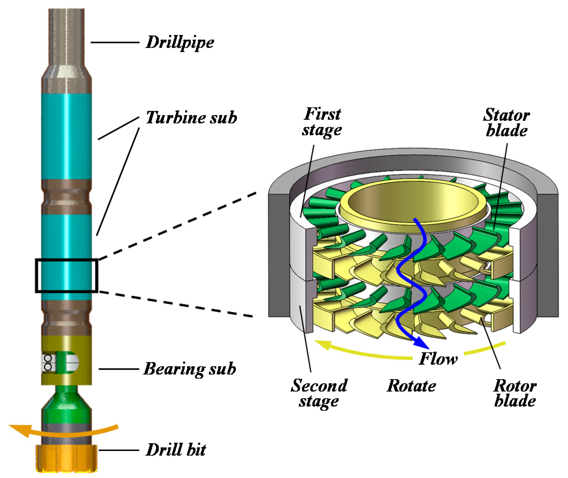
Hot dry rock (HDR) [1] is a renewable clean resource with abundant reserves, and the development of HDR resources can reshape the resource structure, which is beneficial to the sustainable development of the economy, resources, and the environment at large [2]. The bottom of the HDR well hole is a high-temperature and high-pressure environment, and the temperature of the geothermal stratum is high, typically greater than 200 °C and even up to 500 °C [3]. In addition, the huge frictional loss between the slender drill string and the borehole wall causes problems such as a poor surface driving feasibility of the rig and an insufficient strength of the drill pipe. Therefore, it is an inevitable choice to use downhole-powered drilling tools. There are two basic types of downhole driving tools: the screwdrill and the turbodrill [4]. The screwdrill has good mechanical properties, but its rubber stators cannot adapt to the high-temperature working conditions at the bottom of the hole. The all-metal turbodrill has the advantages of high-temperature resistance and corrosion resistance. It is a kind of hydraulic motor driven by the pumped fluid. As shown in Figure 1, drilling fluid transfers its hydraulic power to the mechanical power of the turbine rotor while flowing through the turbine stages. Practical work shows that an all-metal turbodrill with impregnated diamond bits [5] has a good temperature adaptability and a high efficiency in terms of the hard rock [6].
To maintain the stability of deep borehole walls and the stratum, the use of high-density and high-temperature-resistant drilling fluids is possible in HDR wells. High temperatures will affect the flow properties of drilling fluids, which have critical effects on drilling performance [7], including the density, viscosity, shear force, and sand content. The effect of high temperatures on the rheological properties of water-based drilling fluids can be specified by the relationship between temperature and viscosity, which can be divided into three cases: (1) the viscosity decreases as the temperature increases, which is mainly manifested in the reduction of the dynamic shear force of the drilling fluid; (2) solidification occurs after high temperatures, and the drilling fluid loses fluidity; and (3) the viscosity of the drilling fluid decreases first and then increases as the temperature increases. The viscosity range of drilling fluids is between 11.88–35.58 mPa∙s. At the same time, to stabilize the borehole wall and prevent a high-pressure stratum, the density of the drilling fluid can be increased from 1.2 g/cm3 to approximately 1.4 g/cm3 for high-temperature poly-sulfonated drilling fluids drilled in the deep coring of Well Songke-II. Therefore, in view of the flow properties of high-temperature drilling fluids, it is of great significance to develop a theoretical method for the design of high-temperature turbodrills under the conditions of viscous fluid media with two-phase flow.
Wang et al. [8] reviewed recent advances in multiphase flow modeling for Computational Fluid Dynamics (CFD). Seale et al. [9] described the design enhancements made to a turbodrill to accomplish the goals of establishing a shorter tool with more power to address current and future applications. Liu et al. [10] proposed a novel method to optimize the performance of a multi-stage multiphase pump by theoretical prediction based on Oseen vortex and verified the method by CFD. Mokaramian et al. [11] presented numerical simulations of a downhole turbine motor, which were optimized for coiled tube turbodrilling in deep hard rock mineral exploration applications, and studied the CFD simulations of a single-stage turbodrill performance with different rotation speeds and mass flow rates [12]. Beaton [13] described the design enhancements made to the Turbodrill to accomplish the goals of establishing a shorter tool with more power on Coiled Tubing. Andrea et al. [14] performed a fluid-solid coupled simulation by CFD to verify a coupled dynamic model. Wang et al. [15] proposed the law of energy transfer of a turbodrill blade and built a computational model of a single-stage blade on the ANSYS CFD for the Ø127 turbodrill applied in a crystallized section under high-temperature and high-pressure conditions. Mokaramian et al. [16] presented a methodology for designing multistage turbodrills with asymmetric rotor and stator blade configurations, and the simulation results were carried out using a CFD code for the proposed small-size model of the turbodrill stage with different drilling fluid types and various mass flow rates. Hariri et al. [17] investigated the effect of various flow rates, densities, and crude oil viscosities in the steady-state condition of the performance of an industrial turbine flow meter (12 in. with 15 blades), utilizing CFD techniques. Jr et al. [18] considered two different drilling fluid types: sea water and brine and different flow rates to investigate how the velocity vectors, pressure profile, output power, and other performance parameters of the turbodrill are affected. Li [19] studied the energy transmission system of the turbodrill tool using CFX software and discussed the possible influence of the drilling fluid viscosity on the performance of turbine blades. Cusini et al. [20] explored a finite-volume discretization for the multiphase flow equations coupled with a finite-element scheme for the mechanical equations. Betsy et al. [21] carried out CFD analysis to study the fluid-solid coupled effects between blood flow and the stent.
In summary, current research on the design and performance prediction of turbodrill blades is mainly based on the basic principles of axial-flow turbomachinery, using the energy conservation and momentum moment theorems of fluid. There are three main aspects to be improved: (1) The high-temperature and high-density drilling fluid system has a high solid phase content and a large viscosity change at high temperatures. The flow through the blade can no longer be described by an ideal fluid. The current design theory of turbodrill blades based on the Euler equation of ideal fluids is no longer applicable. (2) The application of energy conservation to single-stage blades ignores the effects of two-phase flow and the viscous shear stress of the fluid, resulting in insufficient mathematical models for the output performance of the turbodrill. (3) Turbodrill simulation research is usually aimed at single-stage or below 10 stages, and there are more than one hundred stages of turbodrill blades applied in the field. In this case, the CFD simulation will consider the mutual coupling effects between each stage of the turbodrill to improve the accuracy of the performance prediction.
Based on the flow properties of high-temperature drilling fluids, the basic equation of solid-liquid two-phase flow and the modified Bernoulli equation, a mathematical model for the coupling of two-phase viscous fluid flow with a turbodrill blade is established. A single-stage blade performance prediction model is proposed and extended to multi-stage blades. A 100-stage turbodrill channel model was established using Solidworks. The model was imported into Gambit for meshing. Fluent was used to set the boundary conditions and determine post-processing solutions to obtain the contour diagrams and performance data of the 100-stage turbodrill under different fluid properties, including torque, power, and pressure drop. A comparison of the mathematical models and simulations confirms the influence of two-phase flow, fluid viscosity, and fluid density on the output performance of the turbodrill. The research results help to invert and optimize the design of the basic blade shape and structure of the turbodrill and provide a basis for predicting the actual mechanical properties of high-temperature downhole turbodrills.
2. Model and Methodology
2.1. Hypothesis of the Model
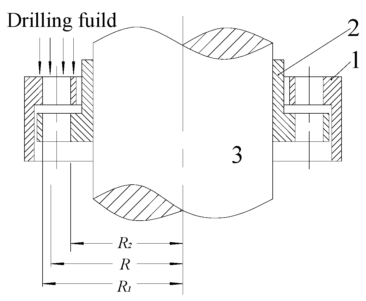
A turbodrill is a non-volume downhole hydraulic motor, the most important of which is the hydraulic component made of the stator and the rotor [22]. Figure 2 shows a schematic diagram of a stator and rotor combination of a single-stage turbodrill blade. When the high-pressure drilling fluid passes through the tunnel, it first flows through the stator blade 1 and then flows out. It interacts with the lower rotor blade 2, and the moment of momentum changes. The mechanical energy of the rotation shaft 3 is obtained, and the drill bit is driven to destroy the rock, thus completing the single-stage blade action. The entire turbodrill power section is composed of hundreds to thousands of single-stage blades stacked in series.
The model is established based on the Navier–Stokes equation of incompressible fluids and the following assumptions: (1) the drilling fluid between the blades is simplified into a solid–liquid two-phase fluid; (2) the pseudo-fluid hypothesis is introduced by assuming that the solid particles dispersed in the fluid are fluids that fill the entire space without gaps; (3) the blades of the turbodrill are smooth and infinitely thin; and (4) there is no flow loss or fluid compression loss out of the stator cylinder.
2.2. Governing Equation of Pseudo-Fluid Solid-Liquid Two-Phase Flow
A two-fluid model (separated flow model) is used here to discuss the basic equations of solid-liquid two-phase flow, where the solid phase is considered as pseudo-fluid.
For the solid phase,
where CS represents the volume concentration of the solid phase in the mixture; is the density of the solid phase; and is the velocity of the solid pseudo-fluid in the direction .
For the liquid phase,
The two equations are added to obtain the continuous equation of the mixture as a whole:
Clearly, the average density of the two-phase mixture is
The equation of motion of the liquid phase also becomes the Navier–Stokes equation of incompressible fluid, as follows:
where VL represents the velocity vector of the liquid phase fluid, p is the pressure of the liquid, µL is the dynamic viscosity of the liquid phase, and FSL is the force vector of the solid phase to the liquid phase in the two-phase flow.
For the solid phase, the equation of motion is
FLS and FSL are the interaction forces between the two phases, with equal magnitudes and opposite directions, including the resistance, the buoyancy caused by the density of the two phases, and the forces caused by the acceleration of the particle’s additional mass.
It can be known from the law of conservation of energy that the rate of change of energy in a system is equal to the sum of the work done by the external force in a unit of time and the heat transferred to it. The energy equation of the viscous fluid expressed by the internal energy is
The constitutive equation of a Newtonian fluid is
Formula (8) can be substituted into (7):
where
Φ is the viscous dissipation function, and it represents the energy dissipation due to the work done by the viscous force. It is given by the expression in the rectangular coordinate system as
For the liquid and solid pseudo-fluid phases, the energy equations follow the formulas derived above. In fact, during the flow of fluid through the turbodrill, it is assumed that the blade wall is smooth, and mechanical energy is lost from the work done by the surface force between the fluid and the wall, including the viscous shear friction between the fluid molecules of the liquid phase, the fluid molecules of the solid phase, and the work done by the interaction forces between the solid and liquid phases.
2.3. Blade Energy Conversion Model Based on Two-Phase Flow
The blade energy conversion model follows the modified Bernoulli equation [3] assuming that the actual turbulent flow is a laminar flow on average. First, the Bernoulli equation for a two-phase flow is given as follows. The energy per unit mass of the liquid in the turbodrill channel is
The energy per unit mass of the solid pseudo-fluid in the turbodrill channel is
The energy per unit mass of the two-phase flow drilling fluid in the turbodrill channel is
When VS = VL,
where and are the mass concentration and volume concentration of the solid phase, respectively, and are the densities of the solid phase and the liquid phase, respectively, and are the velocities of the solid phase and the liquid phase, respectively, and gZ is the potential energy of the position.
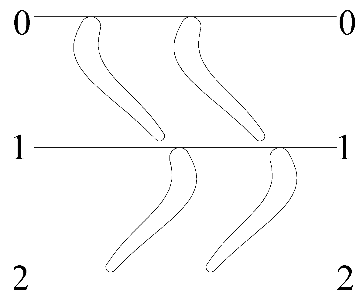
Figure 3 is a planar development view of the stator and rotor blade of the turbodrill, in which the flow routine can be divided into two parts: one is from the stator entrance 0-0 to the stator exit 1-1, and the other is from the rotor entrance 1-1 to the rotor exit 2-2.
In terms of the first stage stator, the pressure energy of the fluid will be transformed into kinetic energy and a partial hydraulic loss due to a lack of mechanic energy output. According to the Bernoulli equation, the energy at the input and output of the turbodrill stator is shown as
where E0 and E1 are the energies of the drilling fluid at the inlet and outlet of the first stage turbodrill stator, respectively; P0 and P1 are the pressures of the drilling fluid at the inlet and outlet of the first stage turbodrill stator, respectively; V0 and V1 are the absolute speeds of the drilling fluid at the inlet and outlet of the first stage turbodrill stator, respectively; Z0 and Z1 are the heights of the drilling fluid at the inlet and outlet of the first stage turbodrill stator, respectively; and hs1 is the mechanical loss of the drilling fluid as it passes through the first stage turbodrill stator.
In terms of the first stage rotor, most energy will transform into mechanical energy and hydraulic loss due to mechanical rotational energy output. According to the Bernoulli equation, the energy at the input and output of the turbodrill rotor is shown as
where E2 is the energy of the drilling fluid at the outlet of the first stage turbodrill rotor; P2 is the pressure of the drilling fluid at the outlet of the first stage turbodrill rotor; V2 is the absolute speed of the drilling fluid at the outlet of the first stage turbodrill rotor; Z2 is the height of the drilling fluid at the outlet of the first stage turbodrill rotor; hr1 is the mechanical loss of the drilling fluid as it passes through the first stage turbodrill rotor; hW is the mechanical energy translated to the rotor; is the energy consumption caused by the centrifugal force component; is the angular velocity; and is the radius of a point on the wall.
According to Formulas (16) and (17), the pressure energy of the first stage stator and rotor and the overall static pressure drop of the stator and rotor can be written as follows:
Repeating the procedures above for a turbodrill with all K stages, all the static pressure drop can be written as
where is the mechanical energy loss of the multi-stage turbodrill blades, and its value is difficult to calculate through formulas and will be obtained through a subsequent numerical simulation analysis of the fluid.
According to the moment of momentum theorem, the torque of the liquid flow acting on the turbodrill shaft in the first stage is
The output torque on the rotation shaft driven by the i stage turbodrill blade is calculated as
In fact, due to the viscosity of the drilling fluid, (21) also needs a viscosity-related term, so that this term is F(µ). When considering the viscosity of the two-phase flow, the conversion torque is
where Mi is the transformation torque of the i stage turbodrill blade, ρ is the average density of the two-phase flow, Q is the average flow rate of the drilling fluid, V(2i−1)u and V(2i)u are the circumferential components of the inlet and outlet speeds of the i stage turbodrill blade, respectively, and F(µ) is a viscosity-related term.
The transfer power of the i stage turbodrill blade is calculated as
For a multi-stage turbodrill, the corresponding torque (power) is the sum of the abovementioned single-stage torque (power), which is
2.4. Simulation Process of the Turbodrill
CFD is the analysis of a system containing fluid flow through computer numerical simulation calculations and image display. By 3D modeling and meshing of the turbodrill blade channel and the subsequent use of CFD software to set the boundary conditions and perform iterative calculations, the speed distribution and pressure distribution of the channels at different speeds can be accurately and intuitively reflected. The performance parameters of the drilling tool are predicted and analyzed, and the cascade design is optimized to improve the hydraulic performance of the designed blade [11].
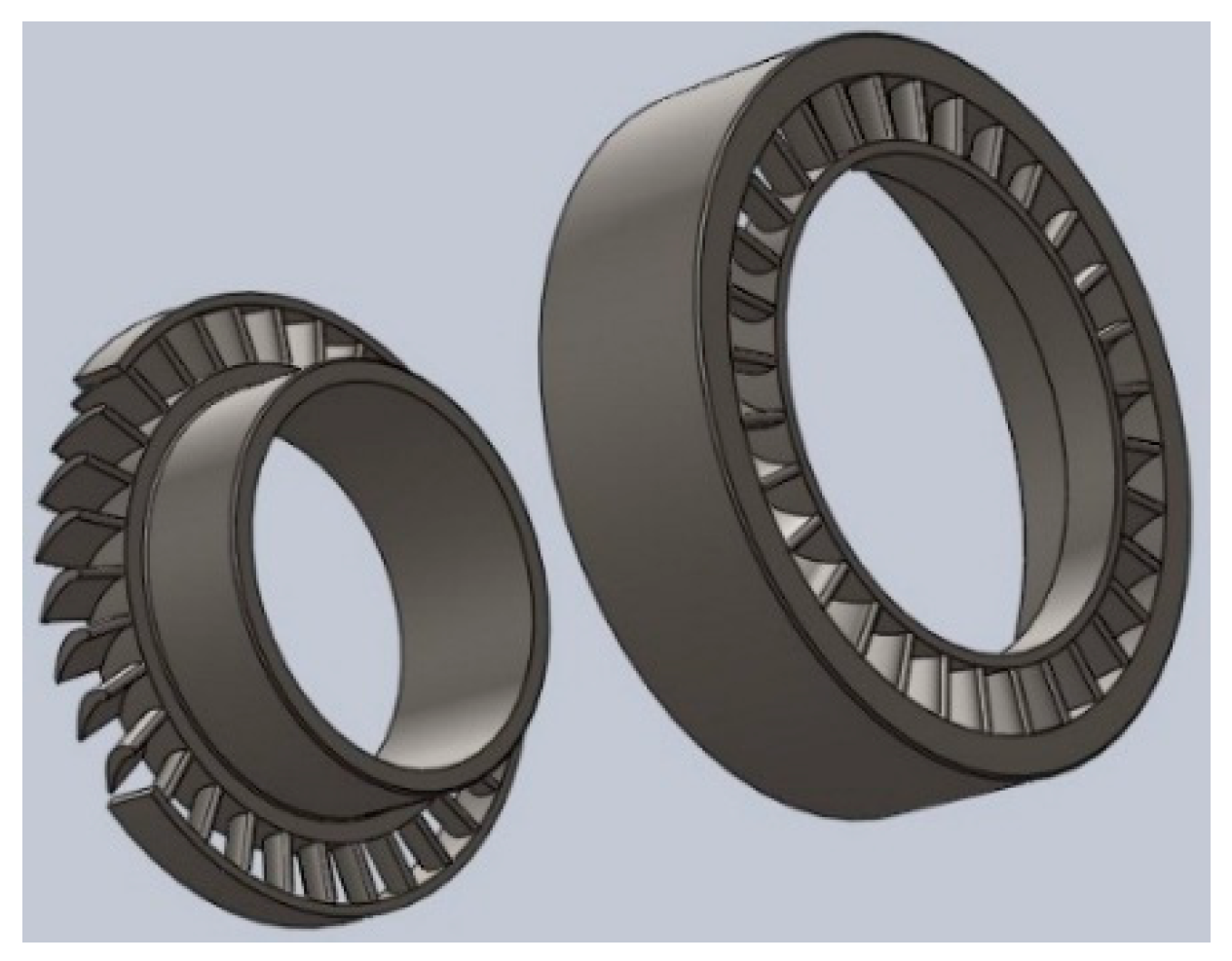
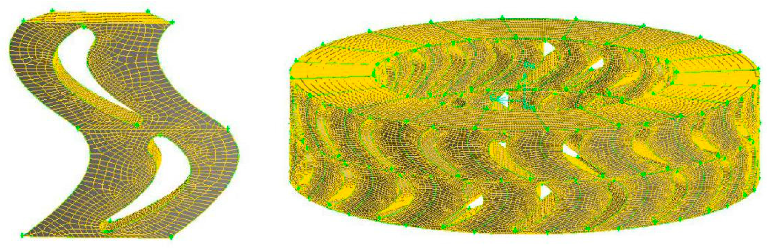
Aiming at the basic structural parameters of the Φ127 mm turbodrill power section, the stator and rotor outer diameter, rim and hub thickness, blade radial height, blade airfoil data points, and a 3D model of the turbine stator and rotor were generated using the Solidworks 3D modeling software. The single-stage and multi-blade model of the turbine is shown in Figure 4.
Due to the periodicity of the stator and rotor in the circumferential direction of the blade, periodic simplification was adopted, and the flow field of only one of the blades (a total of 24 blades) was calculated. At the same time, the stators and rotors of level 100 were completely the same. The grid copy function in the gambit software was used to realize the overall grid of the multi-stage stator and rotor. Because the flow field is a turbulent flow of a three-dimensional viscous fluid, the mesh elements were all hexahedral meshes. For mesh sensitivity, it has been discovered that the simulation results have less fluctuation with the k-ϵ turbulence model [12]. Meanwhile, as the standard k-ϵ model is suitable for general turbulent problems including turbomachinery, it was selected for the following simulation. The mesh independence was considered by comparing the number of cells between whole single-stage turbine, where 1.4 million cells were proven to be enough [23]. In this case, the number of cells in a whole stage was 2.37 million, as shown in Figure 5. So the mesh independence was considered to be satisfied.
To simplify the model, the stator and rotor clearance in the simulation was ignored in this paper. The definition and settings of the model, fluid, and boundary of the channel grid by the Fluent pre-processing software were as follows:
- (1)
- Select the steady-state simulation of the axial turbine. Set up a turbulence model of standard k-ϵ. The solid phase has a density of 2590 kg/m3 and viscosity of 0.05 mPa∙s, and the volume fraction of the solid pseudo-fluid phase is set to 10% for multiphase flow.
- (2)
- Set the regional boundary conditions, including the flow velocity at the stator inlet boundary, the pressure at the rotor outlet, the speed of the rotor area, and the direction of rotation.
- (3)
- The leading and trailing edges of the stator and rotor blades and the blade wall surface rotate with the rotation of the rotor. The speed and direction of the rotor blades remain the same, while the other wall surfaces remain stationary. Therefore, the wall state is set to a non-slip wall state.
- (4)
- Iterative calculation. Select the relaxation factor of the solution, set the residual standard and time step, and use computer multi-core parallel processing to reduce the calculation time.
3. Results and Discussion
3.1. Turbodrill Output Performance Comparison
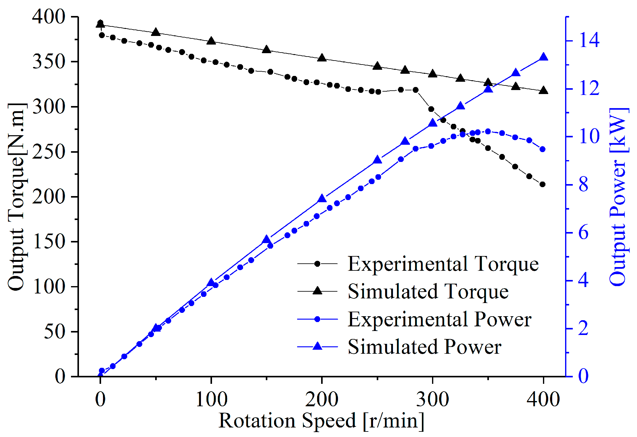
The numerical simulation can obtain the output performance data of the turbodrill including the torque, power, and pressure drop. The simulation results were compared with the performance test data of the 100-stage blades in the article by Wang [15] to verify the new method to predict the overall performance of the turbodrill.
Figure 6 shows a comparison of the turbine stage output performance under simulated and experimental conditions. The experiment took water as the drilling fluid, thus the simulation material was set to 1000 kg/m3 of density. In both cases, the pressure drops of the turbodrill, which are 1.83 MPa and 1.76 MPa, respectively, do not change much with the speed. It can be seen from Figure 6 that the trends of the torque curves obtained by simulation and experiment are basically the same, whose braking torques are 391 N·m and 378 N·m, respectively, and the values are very close. The experimental output power versus speed is basically in a parabolic relationship, and the speed corresponding to the peak power is approximately 350 r/min.
However, as the speed increases, the torque under the experimental conditions tends to decrease faster, causing the torque versus speed to be nonlinear. It is considered that experimental conditions contain friction from ball bearings, which increases with rotation speed. 300 r/min is about the efficient speed for common ball bearings, over which the friction torque will increase greatly with speed. Therefore, the torque versus speed has a greater gradient at speeds more than 300 r/min. In simulations, the mechanical loss is not considered, so torque versus speed remains linear, leading to a larger peak power at a larger speed. Another reason for the difference between the two peak power is that the simplified simulation model gets the shaft power of the turbodrill, while the experimental results are the overall power of the turbodrill. Due to the pulsation of the pump output flow, there is a gap between the output power values in the two cases, especially over 300 r/min. Low-speed turbodrills usually have rated speeds less than 400 r/min, and, therefore, the prediction trend of the 100-stage simulation for the output performance of the turbodrill is correct, and multi-stage simulation can be used as a method for predicting the experimental performance parameters.
3.2. Flow Contour Analysis
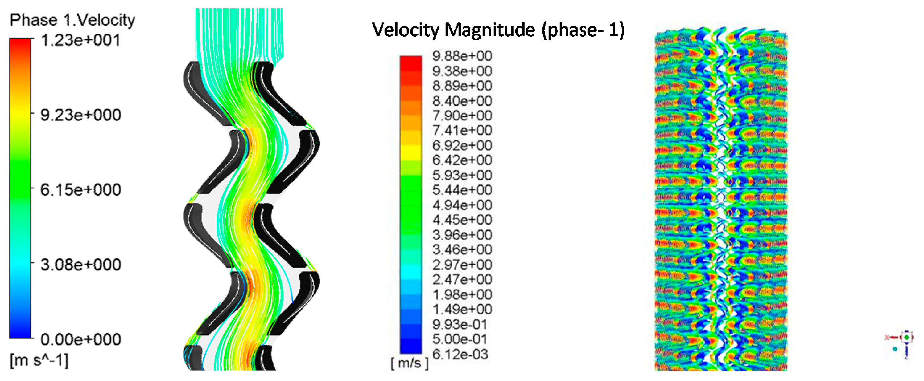
Taking water as the drilling fluid, and the inlet flow rate as 1.5 × 10⁻² m3/s under the speed of 0 r/min; Figure 7 shows a streamline diagram of single-blade multi-stage blades and full-cycle multi-stage blades, with the legend of velocity. As shown in Figure 7, after the drilling fluid entered the blade flow path, the fluid particles basically moved along the blade and separated from the leading edge of the stator. One point flowed to the suction surface of the stator, and the other impacted the pressure surface. The flow velocity at the leading edge of the first stage stator was small. Part of the fluid accelerated to the leading edge of the rotor through the pressure surface of the stator, and the flow velocity gradually increased along the suction surface of the rotor until the maximum curve curvature where the speed reached the peak; the other part flowed directly to the next stage stator through the suction surface of the stator. The velocity of the fluid in the pressure surface of the stator and rotor was significantly higher than that at the suction surface. From the perspective of the blade’s overall flow field, no flow separation occurred.
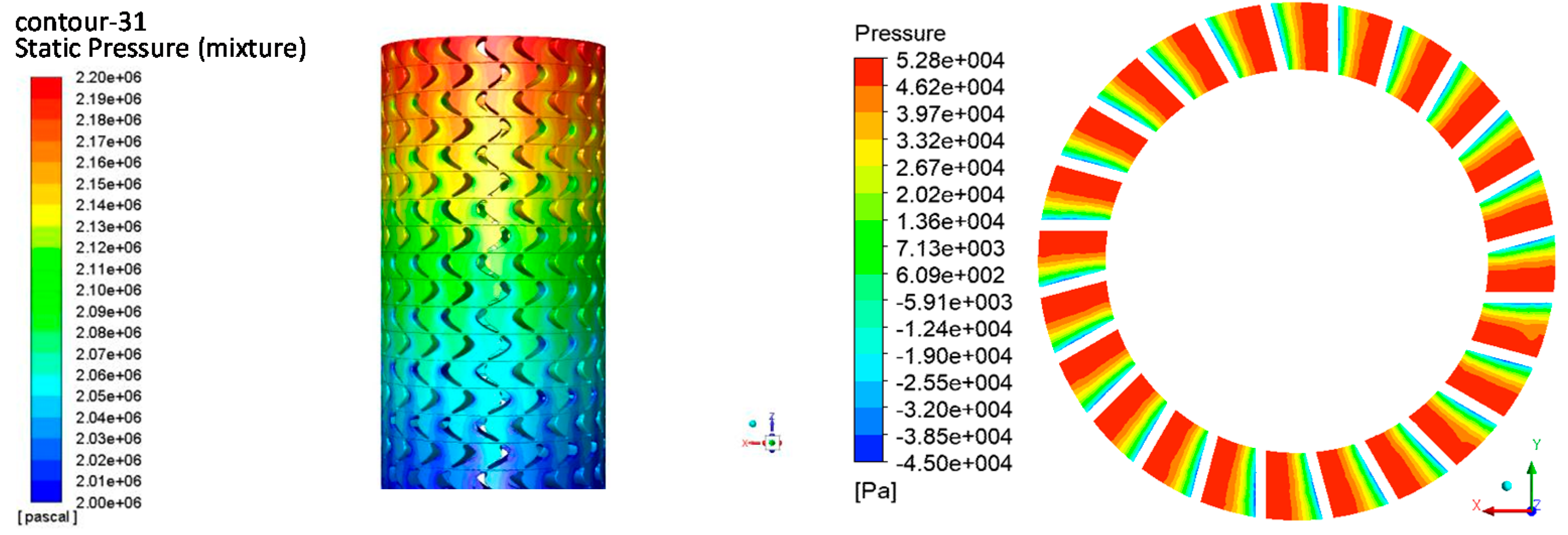
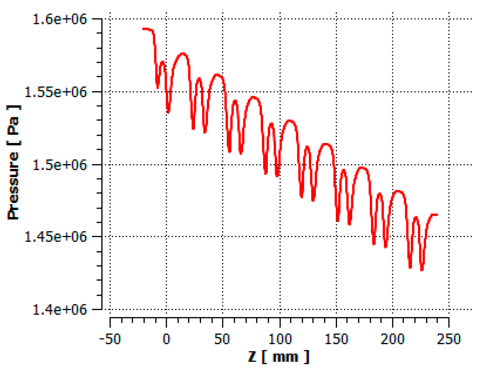
Figure 8 shows the pressure contour diagrams of full-cycle multi-stage turbodrill blades, axially and radially. It can be seen from the figure that the pressure contour diagram of the overall watershed of the 100-stage blades decreased from the first stage to the last stage and there was an obvious pressure gradient in the flow path. Figure 9 shows static pressure versus axial position in a single flow channel. Due to the centrifugal force as Equation (18) indicated, pressure in Figure 9 was lower than that of the outer wall in Figure 8. As the detected axial line passing through the suction surfaces and pressure surfaces, the static pressure fluctuated periodically, but pressure drops in each stage were almost the same, making the static pressure decrease linearly along with the whole turbine. The pressure surface of the blades was higher than the pressure of the suction surface, thereby generating a torque that made the rotor rotate, and energy conversion from pressure energy to mechanical energy was realized.
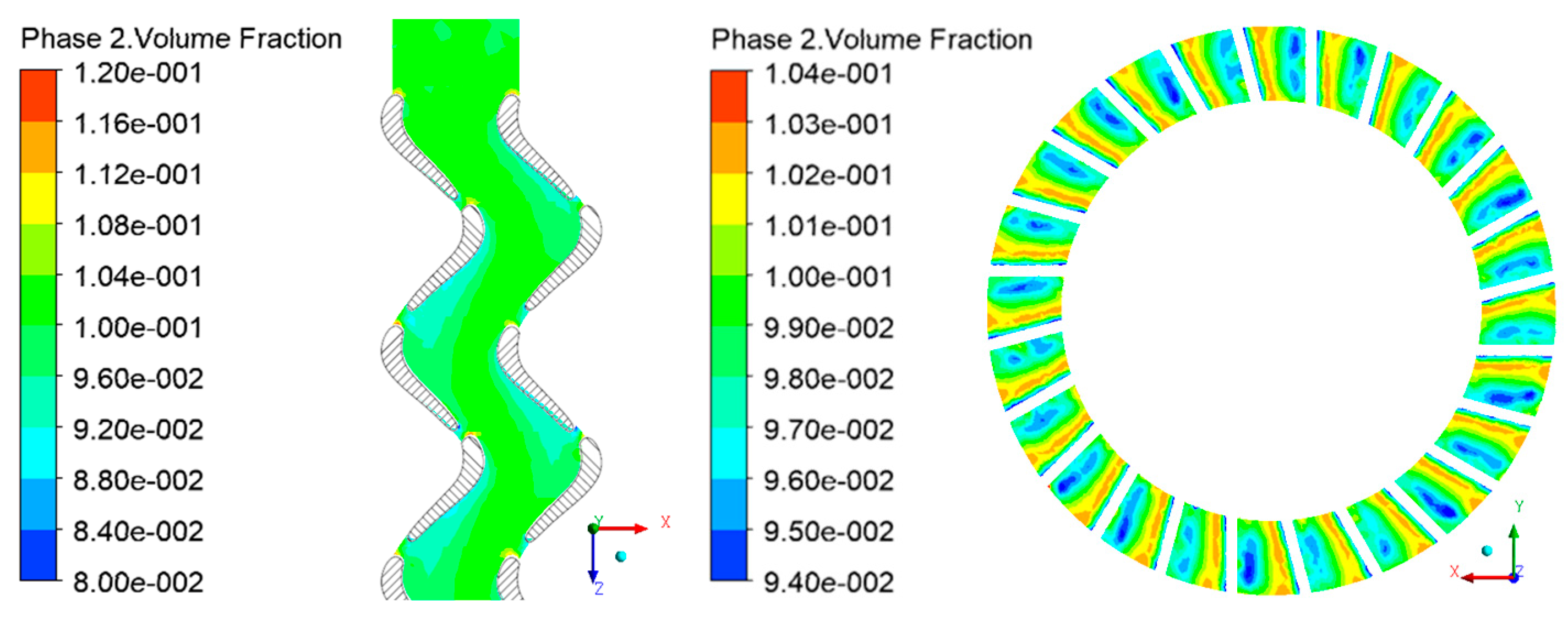
Figure 10 shows the volume fraction contours of the solid pseudo-fluid phase, axially and radially. As the original fraction was 10% from the inlet, the phase distribution slightly changed during the flow. The most concentration occurred at the leading edge of blades, where the flow was blocked. Correspondingly, the volume fraction near trailing edges was the least, indicating the position where the solid phase was unlikely to pass through. The 10% solid phase was in the middle of the flow channel, showing less change in momentum than the water phase. The volume fraction near suction surfaces was less than 10%. This indicates that the solid phase, of more density and viscosity, cannot work as expected as the liquid phase does, which may cause the turbodrill to be less efficient with densified drilling fluid than it was designed. The volume fraction did not vary significantly along the radius.
3.3. Effect of the Drilling Fluid Viscosity on the Turbodrill Output Performance
The change of the viscosity of the drilling fluid is mainly reflected in the change of the dynamic shear force of the liquid phase. According to the mathematical model expression of the pressure drop of the turbodrill blades in Formula (19), the total pressure drop increases as the total mechanical energy loss increases, and most of the mechanical energy loss comes from the shear friction loss caused by the fluid viscosity. According to Formulas (10) and (11), the energy dissipation caused by the viscous force work is positively related to the viscosity of the fluid, so theoretically, an increase in the viscosity of the drilling fluid will cause an increase in the pressure drop in the turbodrill, and the degree of change needs to combine quantitative simulation data.
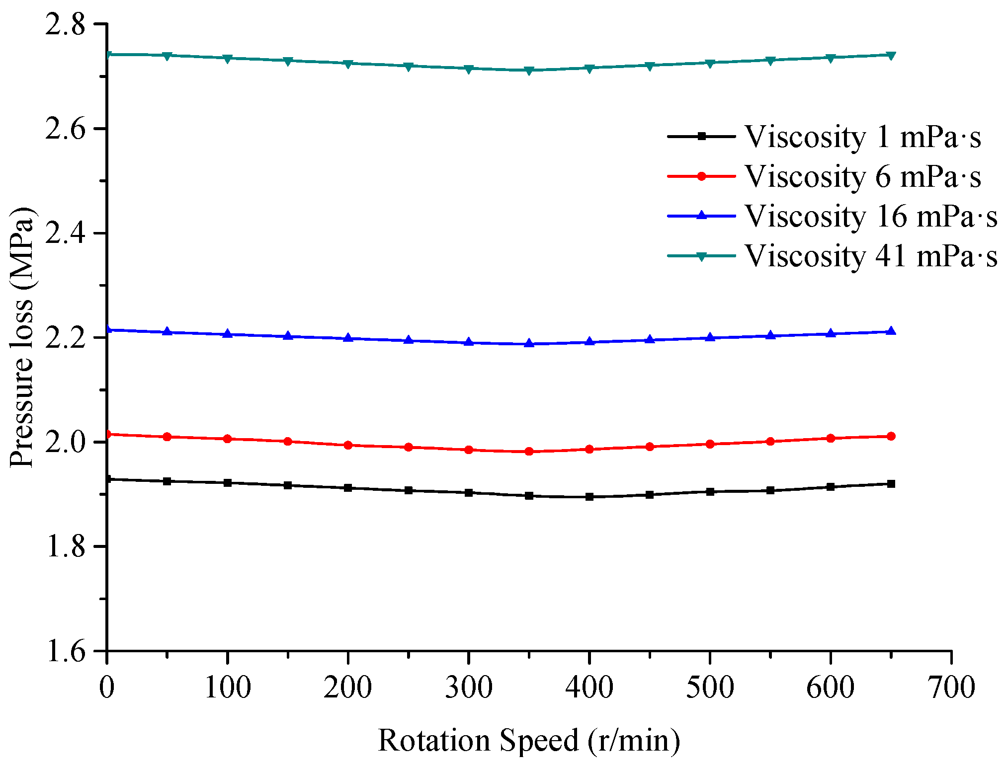
Figure 11 shows the pressure drop vs. speed performance curves for different drilling fluid viscosities (1 mPa·s, 6 mPa·s, 16 mPa·s, 41 mPa·s). The drilling fluid flow rate is 1.5 × 10⁻² m3/s, and the density is 1.16 g/cm3. As shown in Figure 11, the pressure drop of the turbodrill does not substantially change with the rotation speed. Overall, an increase in viscosity increases the pressure drop across the turbodrill. At a viscosity of 1 mPa·s, the pressure drop is 1.92 MPa, and at 41 mPa·s, the corresponding pressure drop is 2.74 MPa, which is an increase of approximately 42.7%. Therefore, the simulation data and the mathematical model reflect the same variation law, and the viscosity of the drilling fluid has a great effect on the pressure drop of the turbodrill.
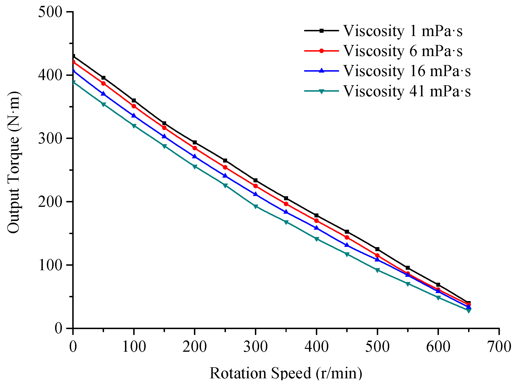
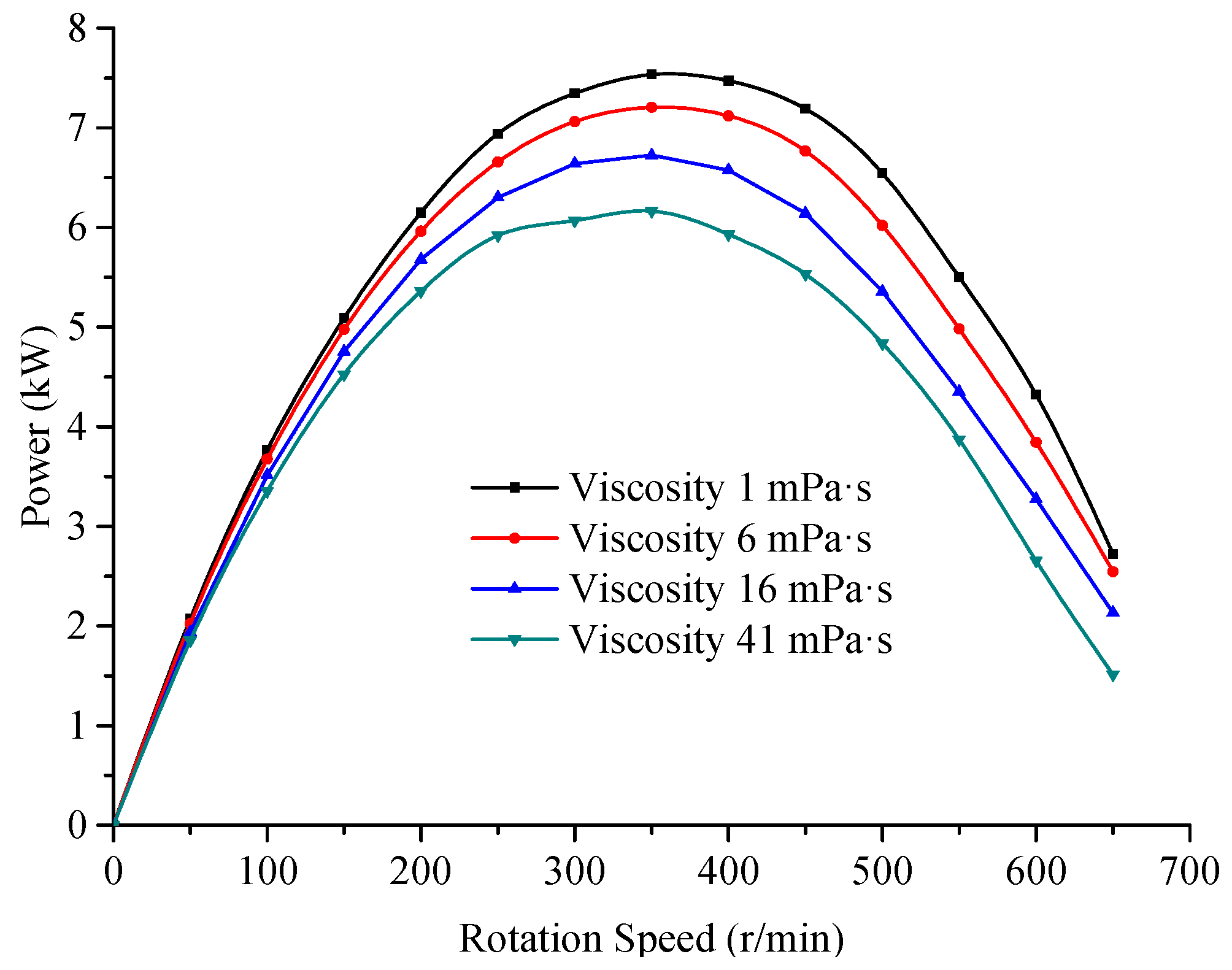
The effect of the drilling fluid viscosity on the turbine-level torque and power is consistent. Based on Formula (24), the influence of the viscous fluid relative to the ideal fluid is the assumed function F(µ). The flow of the three-dimensional viscous fluid along the axis of the turbodrill and the centrifugal rotation relative to the blade are very complicated. Figure 12 is a numerical simulation curve of torque vs. speed under different viscosities, and Figure 13 is a numerical simulation curve of power vs. speed.
According to Figure 12, the torque of the turbine stage is linearly related to the speed. In general, the torque decreases as the viscosity increases, but only slightly. The braking torque is 430 N·m at a viscosity of 1 mPa·s and 389 N·m at a viscosity of 41 mPa·s, a decrease of 9.53%. According to Figure 13, the power decreases as the viscosity increases. When the corresponding power at the four viscosities reached the peak value, the rotation speed was approximately 350 r/min, the peak power was 7.54 kW at a viscosity of 1 mPa·s, and the corresponding power was 6.16 kW at a viscosity of 41 mPa·s, a decrease of 18.31%. Therefore, the viscosity-related term in Formula (24) has a relatively small effect on the torque of the turbodrill. At the optimal operating speed, the power is positively related to the viscosity of the drilling fluid.
The possible reason for this phenomenon is that as the viscosity increases, the Reynolds Number decreases, the degree of turbulence continues to weaken, the laminar flow continues to increase, the kinetic energy of the drilling fluid decreases, and the pressure drop of the turbodrill increases. When the viscosity increases to a certain degree, the Reynolds Number becomes fairly small so that the fluid flowing through the turbodrill channel has mostly become laminar flow. As the viscosity continues to increase, the pressure difference required to promote the same fluid continues to increase at the same speed while the flow characteristic does not change substantially, so the output torque does not change much.
3.4. Effect of the Drilling Fluid Density on the Turbodrill Output Performance
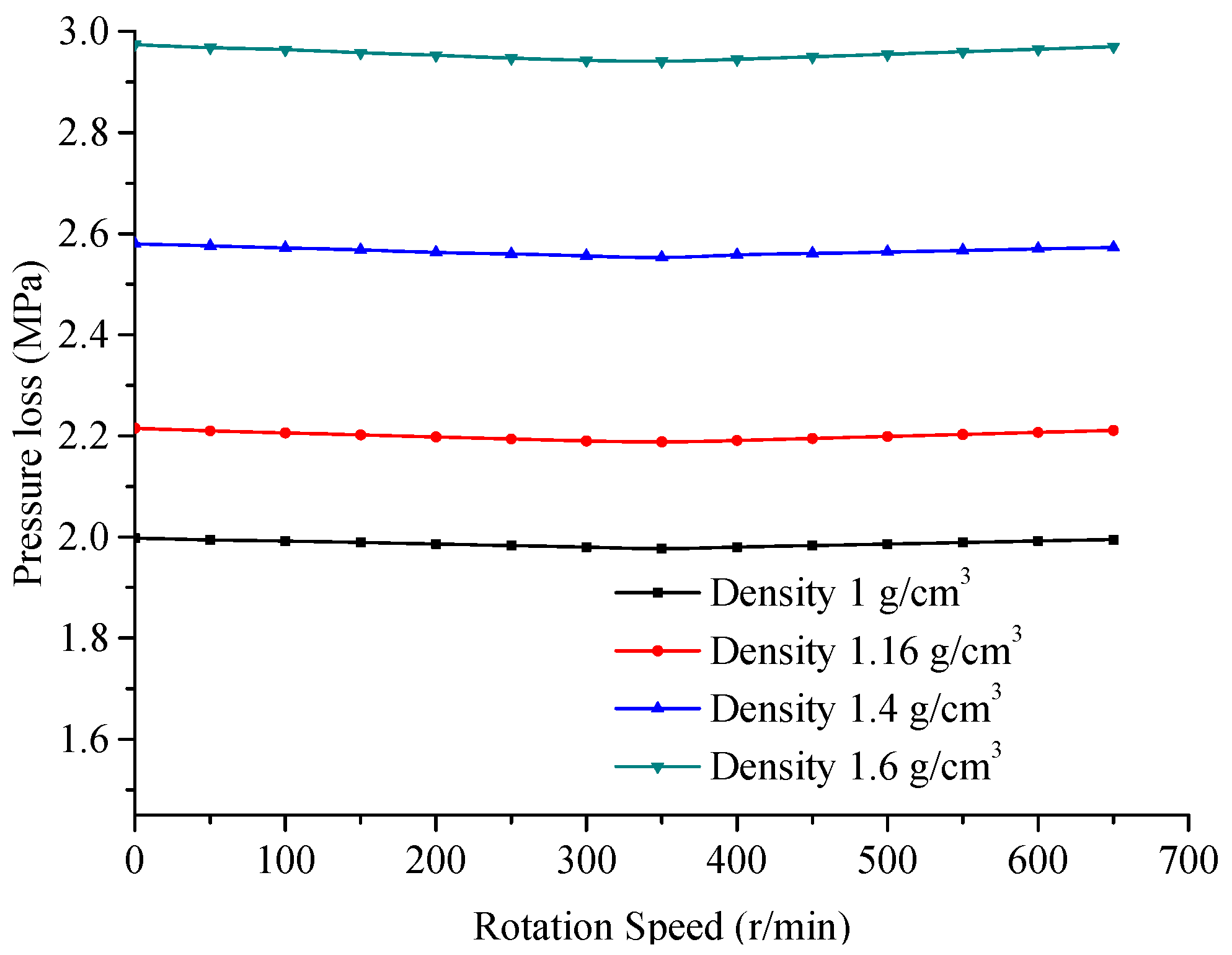
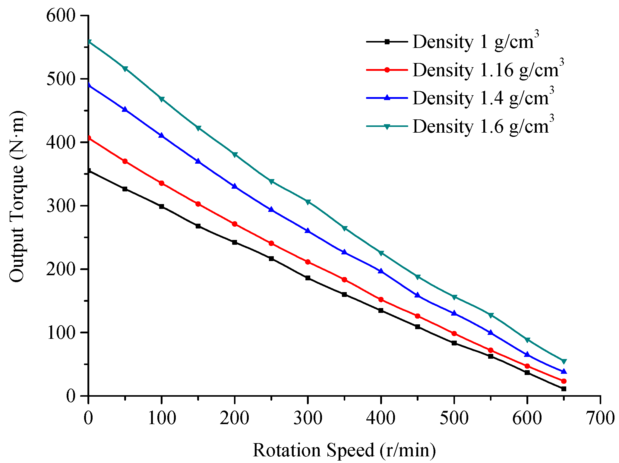
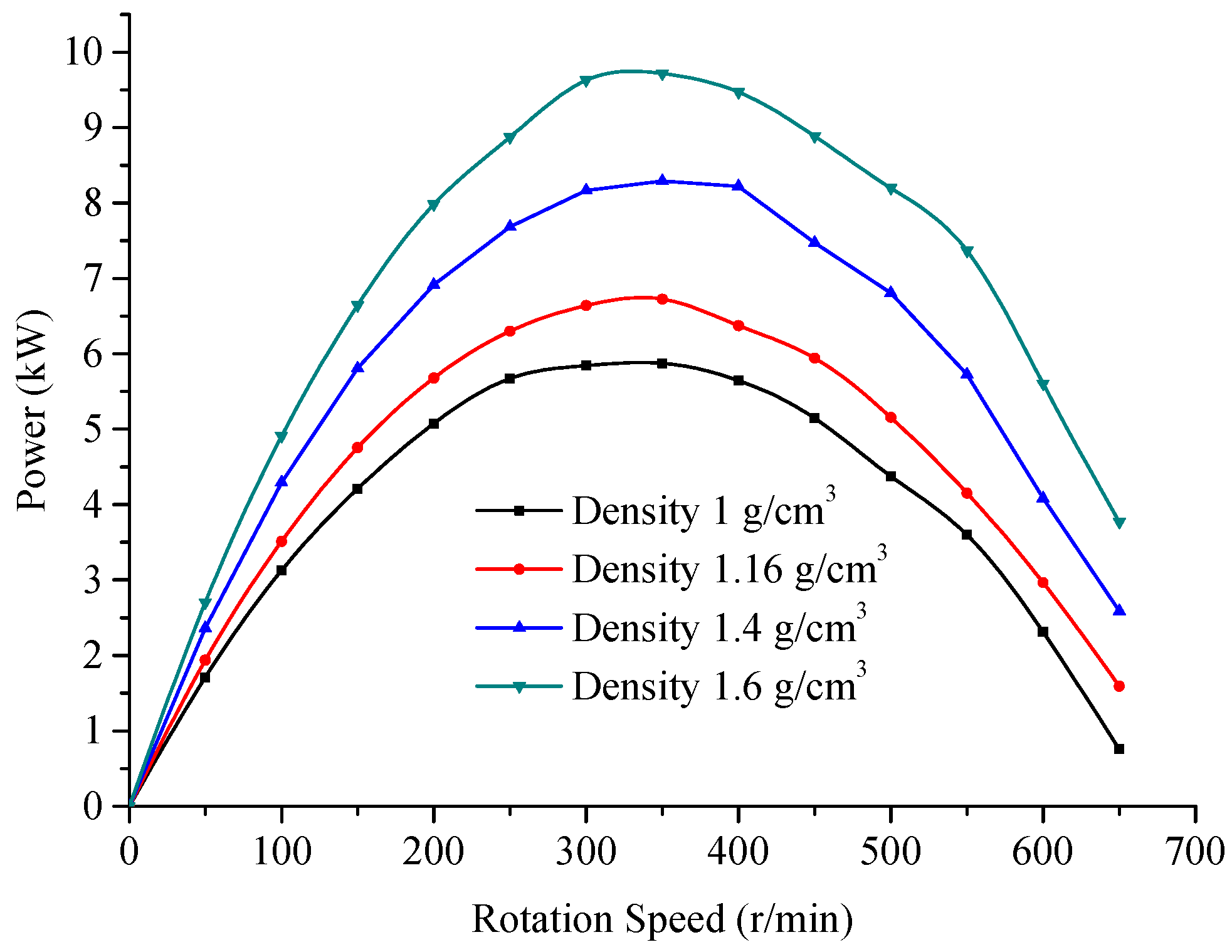
The change of the drilling fluid density is mainly reflected in the site by densifying the drilling fluid, that is, increasing the volume fraction of the solid phase. The mathematical model expression of the pressure drop of the turbine stage is given by Formula (19). The total pressure drop is related to the coefficient , so regardless of whether it increases the liquid phase density, the solid phase density, or the solid phase volume fraction, will lead to an increase in the total pressure drop. At the same time, according to Formula (24), when the average density of the two-phase flow changes, the torque, and power of the turbodrill are positively related to it. Figure 14 shows the pressure drop vs. speed numerical simulation curves under different drilling fluid densities (1 g/cm3, 1.16 g/cm3, 1.4 g/cm3, 1.6 g/cm3), when the flow rate is 1.5 × 10⁻² m3/s and the viscosity is 16 mPa∙s. Figure 15 shows the torque vs. speed curve. Figure 16 shows the power vs. speed curve.
As shown in Figure 14, the increase in density will increase the pressure drop of the turbodrill. The pressure drop at a density of 1 g/cm3 is approximately 2 MPa, and the corresponding pressure drop at 1.6 g/cm3 is 2.95 MPa, an increase of approximately 47.5%. As shown in Figure 15 and Figure 16, when the average density of the two phases is increased from 1 g/cm3 to 1.6 g/cm3, the braking torque and peak power are increased by 56.3% and 65.6%, respectively. Therefore, the simulation data confirm the law of the mathematical model very well: an increase in the drilling fluid density will greatly increase the torque and power and improve the performance of the turbodrill. At the same time, the pressure drop will also increase, which is not good for drilling.
4. Conclusions
In this paper, based on the basic equations of solid-liquid two-phase flow and the modified Bernoulli equation, a mathematical model of turbodrill blade energy transmission was established, considering the fluid properties. The mathematical model shows that the viscosity of the drilling fluid does not have a very large effect on the torque and power of the turbodrill, but the increase in viscosity will greatly increase the pressure drop consumed by the turbodrill, thereby reducing the working efficiency. A 100-stage turbodrill channel fluid model was established, which improved the multi-stage and multi-blade simulation method. The simulation results were verified by the existing experimental results. The effects of fluid viscosity, and fluid density on the output performance of the turbodrill were qualitatively analyzed. The numerical simulation results show that aggravating the drilling fluid can significantly increase the torque and power and improve the performance of the drilling tool, but at the same time, it will increase the pressure drop of the hydraulic components. Therefore, the composition of the drilling fluid should be reasonably configured. For the drilling fluid, conditions of medium viscosity (16 mPa·s) and medium density (1.6 g/cm3) are more conducive to the optimal operation of the turbodrill.
Author Contributions
D.Z. and Y.W. wrote the paper. J.S. carried out the numerical simulations. Y.H. reviewed the paper. All authors have read and agreed to the published version of the manuscript.
Funding
This work is supported by the National Natural Science Foundation of China (No. 41872180, 41802197), the Fundamental Research Funds for the Central Universities (No. 292018093), and the National Key R&D Program of China (No. 2018YFC0603404).
Institutional Review Board Statement
Not applicable.
Informed Consent Statement
Not applicable.
Data Availability Statement
Data sharing not applicable.
Acknowledgments
We sincerely acknowledge the previous researchers for their excellent work, which greatly assisted our academic study.
Conflicts of Interest
The authors declare that there is no conflict of interests regarding the publication of this paper.
References
- Frash, L.P.; Gutierrez, M.; Hampton, J. True-triaxial apparatus for simulation of hydraulically fractured multi-borehole hot dry rock reservoirs. Int. J. Rock Mech. Min. Sci. 2014, 70, 496–506. [Google Scholar] [CrossRef] [Green Version]
- Zhang, D.L.; Weng, W.; Zhao, C.L. Development and application of turbodrills in hot dry rock drilling. J. Groundw. Sci. Eng. 2018, 6, 1–6. [Google Scholar]
- Wang, Y.; Xia, B.; Wang, Z.; Wang, L.; Zhou, Q. Design and output performance model of turbodrill blade used in a slim borehole. Energies 2016, 9, 1035. [Google Scholar] [CrossRef] [Green Version]
- Sergey, L.S. Turbodrill and screw motor: Development dialectics. In Proceedings of the SPE Russian Petroleum Technology Conference and Exhibition, Moscow, Russia, 24–26 October 2016. [Google Scholar]
- Pantoja, R.; Britto, G.; Buzzá, J. Pioneer turbodrilling with 16 ½ impregnated bit in deep pre-salt well in Santos basin. In Proceedings of the SPE/IADC Drilling Conference and Exhibition, London, UK, 17–19 March 2015. [Google Scholar]
- Wang, Y.; Liu, B.L.; Zhu, H.Y. Thermophysical and mechanical properties of Granite and its Effects on Borehole Stability in High Temperature and Three-dimensional Stress. Sci. World J. 2014, 2014, 650683. [Google Scholar]
- Abazariyan, S.; Rafee, R.; Derakhshan, S. Experimental study of viscosity effects on a pump as turbine performance. Renew. Energy 2018, 127, 539–547. [Google Scholar] [CrossRef]
- Wang, J.; Vujanovic, M.; Sunden, B. A review of multiphase flow and deposition effects in film-cooled gas turbines. Therm. Sci. 2018, 22, 1905–1921. [Google Scholar] [CrossRef]
- Seale, R.; Beaton, T.; Flint, G. Optimizing turbodrill designs for coiled tubing application. In Proceedings of the SPE Eastern Regional Meeting, SPE-91453-MS, Charleston, WV, USA, 15–17 September 2004; pp. 1–10. [Google Scholar]
- Liu, M.; Tan, L.; Xu, Y.; Cao, S.L. Optimization design method of multi-stage multiphase pump based on Oseen vortex. J. Pet. Sci. Eng. 2020, 184, 106532. [Google Scholar] [CrossRef]
- Amir, M.; Vamegh, R.; Gary, C. CFD simulations of turbodrill performance with asymmetric stator and rotor blades congiguration. In Proceedings of the Ninth International Conference on CFD in the Minerals and Process Industries CSIRO, Melbourne, Australia, 10–12 December 2012. [Google Scholar]
- Amir, M.; Vamegh, R.; Gary, C. Fluid Flow Investigation through Small Turbodrill for Optimal Performance. Mech. Eng. Res. 2013, 3, 1–24. [Google Scholar]
- Beaton, T.; Seale, R. The use of turbodrills in coiled tubing applications. In Proceedings of the SPE/ICoTA Coiled Tubing Conference and Exhibition, Houston, TX, USA, 23–24 March 2004. [Google Scholar]
- Andrea, D.M.; Giovanni, J.; Massimo, S. Optimization of gerotor pumps with asymmetric profiles through an evolutionary strategy algorithm. Machines 2019, 7, 17. [Google Scholar]
- Wang, Y.; Yao, J.Y.; Li, Z.J. Design and development of turbodrill blade used in crystallized section. Sci. World J. 2014, 2014, 682963. [Google Scholar]
- Mokaramian, A.; Rasouli, V.; Cavanough, G. Turbodrill design and performance analysis. J. Appl. Fluid Mech. 2015, 8, 377–390. [Google Scholar] [CrossRef]
- Hariri, S.; Hashemabadi, S.H.; Noroozi, S. Analysis of operational parameters, distorted flow and damaged blade effects on accuracy of industrial crude oil turbine flow meter by CFD techniques. J. Pet. Sci. Eng. 2015, 127, 318–328. [Google Scholar] [CrossRef]
- Sampaio, J.H.B., Jr.; Monteiro, V.G.; Tomita, J.T. Performance evaluation of a hydraulic turbine used as a turbodrill for oil and gas applications in post-salt environment. In Proceedings of the ASME Turbo Expo: Turbomachinery Technical Conference and Exposition, Charlotte, NC, USA, 26–30 June 2017. [Google Scholar]
- Li, Y. Energy Transmission System and Blade Shap Optimization of Turbodrill. Master’s Thesis, Harbin Institute of Technology, Harbin, China, 2021. [Google Scholar]
- Cusini, M.; White, J.A.; Castelletto, N.; Settgast, R.R. Simulation of coupled multiphase flow and geomechanics in porous media with embedded discrete fractures. Int. J. Numer. Anal. Methods Geomech. 2020. [Google Scholar] [CrossRef]
- Betsy, D.M.; Fabio, S.; Daniele, C. A smart stent for monitoring eventual restenosis: Computational fluid dynamic and finite element analysis in descending thoracic aorta. Machines 2020, 8, 81. [Google Scholar]
- Eskin, M.; Maurer, W.C. Advanced Downhole Drilling Motors; Maurer Engineering Inc.: Houston, TX, USA, 1997. [Google Scholar]
- Khaled, S.; Abderrahmane, B.; Ahmed, S.M.; Rekik, O. Flow simulation and performance analysis of a drilling turbine. J. Eng. Res. 2020, 8, 255–270. [Google Scholar]
Figure 1.
Typical turbodrill schematic.

Figure 2.
Sketch of the turbodrill blade assembly. 1. Stator blade 2. Rotor blade 3. Rotation shaft.
Figure 2.
Sketch of the turbodrill blade assembly. 1. Stator blade 2. Rotor blade 3. Rotation shaft.

Figure 3.
Drilling fluid flow in the turbodrill blade.

Figure 4.
Single-stage and multi-blade turbodrill stator and rotor model.

Figure 5.
Single blade and full channel meshing model.

Figure 6.
Comparison of turbodrill output performance under simulated and experimental conditions.

Figure 7.
Streamline diagram of single−blade multi−stage turbodrill blades.

Figure 8.
Pressure contour diagram of full−cycle multi−stage turbodrill blades.

Figure 9.
Static pressure in the first 8−stage blades’ channel.

Figure 10.
Volume fraction contour of turbodrill stages.

Figure 11.
Pressure drop vs. speed curves for different viscosities.

Figure 12.
Torque vs. speed curves for different viscosities.

Figure 13.
Power vs. speed curves for different viscosities.

Figure 14.
Pressure drop vs. speed curves at different densities.

Figure 15.
Torque vs. speed curves at different densities.

Figure 16.
Power vs. speed curves at different densities.

Publisher’s Note: MDPI stays neutral with regard to jurisdictional claims in published maps and institutional affiliations. |
© 2021 by the authors. Licensee MDPI, Basel, Switzerland. This article is an open access article distributed under the terms and conditions of the Creative Commons Attribution (CC BY) license (https://creativecommons.org/licenses/by/4.0/).
Share and Cite
MDPI and ACS Style
Zhang, D.; Wang, Y.; Sha, J.; He, Y. Performance Prediction of a Turbodrill Based on the Properties of the Drilling Fluid. Machines 2021, 9, 76. https://doi.org/10.3390/machines9040076
AMA Style
Zhang D, Wang Y, Sha J, He Y. Performance Prediction of a Turbodrill Based on the Properties of the Drilling Fluid. Machines. 2021; 9(4):76. https://doi.org/10.3390/machines9040076
Chicago/Turabian StyleZhang, Delong, Yu Wang, Junjie Sha, and Yuguang He. 2021. "Performance Prediction of a Turbodrill Based on the Properties of the Drilling Fluid" Machines 9, no. 4: 76. https://doi.org/10.3390/machines9040076
Note that from the first issue of 2016, this journal uses article numbers instead of page numbers. See further details here.