

Tool Wear State Identification Based on the IWOA-VMD Feature Selection Method
1
School of Mechanical Automation, Wuhan University of Science and Technology, Wuhan 430081, China
2
Key Laboratory of Metallurgical Equipment and Its Control, Ministry of Education, Wuhan University of Science and Technology, Wuhan 430081, China
*
Author to whom correspondence should be addressed.
Machines 2024, 12(3), 184; https://doi.org/10.3390/machines12030184
Submission received: 29 January 2024
/
Revised: 22 February 2024
/
Accepted: 23 February 2024
/
Published: 12 March 2024
(This article belongs to the Topic Uncertainty Quantification in Design, Manufacturing and Maintenance of Complex Systems)
Abstract
:Complex, thin-walled components are the most important load-bearing structures in aircraft equipment. Monitoring the wear status of milling cutters is critical for enhancing the precision and efficiency of thin-walled item machining. The cutting force signals of milling cutters are non-stationary and non-linear, making it difficult to detect wear stages. In response to this issue, a system for monitoring milling cutter wear has been presented, which is based on parameterized Variational Mode Decomposition (VMD) Multiscale Permutation Entropy. Initially, an updated whale optimization technique is used, with the joint correlation coefficient serving as the fitness value for determining the VMD parameters. The improved VMD technique is then used to break down the original signal into a series of intrinsic mode functions, and the Multiscale Permutation Entropy of each effective mode is determined to generate a feature vector. Finally, a 1D Convolutional Neural Network (1D CNN) is employed as the input model for state monitoring using the feature vector. The experimental findings show that the suggested technique can efficiently extract characteristics indicating the wear condition of milling cutters, allowing for the precise monitoring of milling cutter wear states. The recognition rate is as high as 98.4375%, which is superior to those of comparable approaches.
1. Introduction
The aircraft industry has a significant need for multiple thin-walled components with high machining accuracy, such as aero-engine impellers and blades. The surface integrity and geometric tolerances of these thin-walled components are inextricably linked to the state of the cutting tools. As a result, the real-time and exact monitoring of tool wear during the machining process of thin-walled components is critical for improving machining precision and productivity. Current methodologies for the monitoring cutting tool status are divided into two categories: direct inspection techniques and indirect inspection techniques [1]. Currently, the most common direct monitoring approach is machine vision, but the technology is costly, and the picture is readily altered by on-site processing circumstances [2]. Indirect procedures include the extraction of implicit parameters related to tool deterioration from cutting signals collected by field sensors. The relationship between these implicit traits and tool deterioration is established using machine learning and deep learning techniques, allowing for the real-time monitoring of tool degradation. Sensors now collect physical signals associated with the states of the cutting tools, such as cutting forces [3,4], electrical current and power [5,6], acoustic emission (AE) [7,8], auditory signals [9,10], and vibrational signals [11,12]. Of these signs, cutting force has been proven to be the most reliable and widely used method for predicting tool wear [13].
However, when utilizing the cutting force signal to determine the milling tool’s deterioration condition, noise is frequently intermingled with the signal acquired on the spot, making signal processing critical. Wavelet Analysis [14,15] and Empirical Mode Decomposition (EMD) [16,17] are two commonly used signal processing approaches that have been successfully employed to detect milling tool damage. Wavelet Analysis is effective in extracting wear characteristics from non-linear and non-stationary tool deterioration data. However, considerable technical knowledge is required when determining the proper basis function, since this will affect the efficacy of extracting milling cutter wear characteristics. EMD is a self-adaptive technique for processing non-linear and non-stationary signals, eliminating the need for basis functions. However, there are issues with the EMD decomposition method, including modal confusion and endpoint effect [18], as well as a weak anti-noise capacity. Dragomiretskity et al. [19] introduced a unique approach of Adaptive Variational Mode Decomposition (VMD) that addresses the problems of the end effect and modal aliasing for EMD while also having a high anti-noise capacity. It has been used to cut chatter monitoring [20,21]. However, using the VMD method to deconstruct cutting force signals requires pre-setting the decomposition iterations and penalty factor. Currently, the most often utilized approaches are the center frequency observation method [22] and the intelligent optimization algorithm for parameter optimization [23]. The former is heavily influenced by subjective variables and has limited flexibility. The latter has an issue with establishing the parameters for the fitness function and the optimization process. Currently, a wide range of meta-heuristic techniques have been successfully used to solve the issue of VMD parameter optimization. Among these optimization methods, the whale optimization (WOA) [24] algorithm has gained popularity because of its quick convergence time, minimal control parameters, and ease of implementation. However, when looking for a near-global optimum, there is still the issue of diminished population variety and a tendency to settle for local optima. To solve this issue, the elite reverse learning approach is used to choose individuals with a high fitness for the following iteration, thereby enhancing the original population quality. The golden sine algorithm is introduced to improve the spiral upward predation of the whales, resulting in a faster rate of convergence for the algorithm. To efficiently determine the best parameters for VMD, the least joint correlation coefficient is employed as the objective function, and an IWOA-VMD-based approach is used to extract wear feature information from the milling cutter’s cutting force signal.
After decomposing the milling cutter’s cutting force signal using the IWOA-VMD approach, the resulting Intrinsic Mode Functions (IMFs) include a plethora of feature information on the milling cutter’s wear. The IMFs’ feature information is adequately described through the addition of entropy theory. Entropy-based techniques, such as Fuzzy Entropy, Approximate Entropy, and Sample Entropy, have been widely utilized to monitor milling cutter noise [25,26,27]. Peng et al. [28] presented a system for vibration detection based on Optimized Variational Mode Decomposition and Fuzzy Entropy, to realize vibration surveillance. Yang et al. [29] used Approximate Entropy and Sample Entropy as vibration indices to identify vibrations under various machining settings. However, the value of approximation entropy is heavily influenced by the length of the data; particularly when working with short data, its estimate typically falls short of the expected value [18]. Although the Sample Entropy and Fuzzy Entropy techniques are intended to reduce the dependence on data length, they are computationally inefficient for processing large amounts of data. To address these issues, Bandt et al. [30] proposed a new entropy, Permutation Entropy (PE), for measuring signal complexity. Its computation technique is straightforward and ideal for online monitoring. However, the intrinsic non-stationary and time-varying properties of cutting force signals generated by milling tools are often wrapped inside a multiscale sequence. The extraction of these properties exclusively through Permutation Entropy has inherent limitations. Multiscale Permutation Entropy (MPE) may extract multiscale aspects of signals based on the time series, allowing for a full characterization of the underlying information in cutting force signals. This approach, known for its durability and high operational speed, has found widespread use in chatter detection [31,32].
Choosing an effective approach for state recognition is also critical in terms of signal processing and feature vector creation. Given the considerable improvements that deep learning has made across a wide range of fields, it is particularly interesting that Convolutional Neural Networks (CNNs) are the most often used methodology within the realm of deep learning approaches. CNNs have been widely employed for monitoring tool wear conditions [33] due to their inherent capacity to incorporate feature extraction and classification, together with adaptive feature filtering, as opposed to standard machine learning models [34]. Yang et al. [35] presented a system for tool wear monitoring based on multivariate cutting force and a 1D CNN, which demonstrated higher precision in recognizing the degradation condition of milling tools. Lu et al. [36] incorporated an Adaptive Frequency Band Attention Module (AFBAM) into the CNN model. This module adaptively amplifies the frequency bands with the most vibration information by analyzing the signal’s time–frequency characteristics.
Because of the inherent non-linear and non-stationary characteristics of the cutting force signals produced by milling tools, determining the status of tool wear is a significant difficulty. In this paper, a milling cutter wear state recognition method based on parameter optimization VMD multi-scale permutation entropy is proposed. First, the elite reverse learning and golden sine algorithms are used to enhance the WOA, and the IWOA is constructed to optimize the VMD parameters by using the joint correlation coefficient as a fitness value. The original signal is then decomposed into several IMFs using the IWOA-VMD method. The correlation coefficient is then calculated between each IMF and the original signal, and then the MPE value is computed for the IMFs that have a significant connection with the original signal. This is then utilized to create the feature vector. Finally, a proposal is provided for using a one-dimensional Convolutional Neural Network as the input model for milling cutter wear condition detection. The main contributions of this study are as follows:
- (1)
- An approach for refining VMD parameters is provided, based on the IWOA. To address the issues of a slow convergence velocity and the tendency to slip into local optima, an IWOA method based on elite inverse learning and the golden sine algorithm is presented. The IWOA technique is used to investigate the ideal parameter combinations for VMD by minimizing the joint correlation coefficient in using modal components.
- (2)
- In leveraging its capabilities, it is proposed to incorporate Multiscale Permutation Entropy into the feature extraction process for milling tools, resulting in a more robust representation of feature information.
- (3)
- A one-dimensional CNN was used to filter wear characteristics and determine the conditions of milling cutters. This technique ensures milling tool wear monitoring precision while decreasing the 1D CNN’s training parameters.
- (4)
- The approach’s efficacy was confirmed through testing on the 2010PHM public dataset.
2. Milling Cutter Wear Feature Extraction
2.1. Variational Mode Decomposition
The variational mode decomposition algorithm is a signal decomposition approach that may be both adaptive and quasi-orthogonal, allowing it to avoid end-point effects and spurious components during iteration. The VMD algorithm redefines the IMFs as an AM-FM signal, as shown in Equation (1):
where is the modal component; is its envelope amplitude; and is its instantaneous phase.
The marginal spectrum is obtained using the Hilbert transform and shifted to the baseband for each , and the bandwidth is estimated using the VMD on the squared parameter L2 of the signal’s gradient to derive the expression for the variational problem, as shown in Equation (2):
which stands for the K mode components; corresponds to the center frequencies of each ; is the Dirac function; e indicates the convolution operation; and refers to the original signal.
To solve the optimal solution issue, the Lagrange multiplier and the quadratic penalization factor are introduced, with the enhanced Lagrange expression represented in Equation (3):
In order to obtain the optimal solution, the alternating direction multiplication operator is used to solve the problem. The iterative steps are as follows:
- (1)
- Initialize , and n = 0.
- (2)
- N = n+1, enter the loop.
- (3)
- , , and are updated based on the updated Equation (6), and the inner loop is terminated once the decomposition count hits K.
- (4)
- Stop the loop given the discriminative accuracy ; otherwise, go back to step (2) and continue to execute the previously described steps until the conditions for iteration cessation are fulfilled.
2.2. IWOA Optimization of VMD
2.2.1. IWOA
Mirjalili and colleagues first introduced the whale optimization method (WOA), a novel method for swarm intelligence optimization, in 2016 [37]. It is congruent with intelligent algorithms, which are often inspired by the properties of biological organisms and their natural behaviors. The WOA represents a swarm intelligence-based heuristic approach to global optimization. It is a proposed algorithm that simulates the social behavior of humpback whales in the ocean when rounding up prey and introduces a bubble net hunting strategy, which is typically used to find the optimal solution. This study uses the properties of the WOA to discover the ideal parameters for the VMD algorithm, ensuring that the VMD’s decomposition impact fulfills expectations. The whale optimization method is made up of three major components: rounding up prey, bubble attack, and discovering prey.
The objective of the Elite Inverse Learning Strategy [38] is to augment the heterogeneity within the initial population. The traditional whale optimization algorithm uses random generation to generate the initial population, resulting in the initial population’s adaptability being low, which directly affects the effect of the later iterations. The elite reverse learning strategy generates a reverse population on the basis of the randomly generated population, calculates the population with the best fitness function value to serve as the beginning population for the next iteration, and the mathematical notation for producing the reverse population is as follows:
In Equation (4), is a random number in [0,1], is the maximum value of the position vector in the initial population, is the minimum value of the position vector in the initial population, and change with the increase in iteration number, is the position vector in the initial population, and is the position vector in the corresponding reverse population. The position vectors in the reverse population are examined using the constraints, and the position vectors that do not satisfy the constraints are randomly generated, and the mathematical publicity of the randomly generated position vectors is shown in Equation (5):
Tanyildizi et al. presented the golden sine algorithm [39] in 2017, which optimizes the position updating approach. The algorithm employs the sinusoidal function in mathematics for a computational, iterative optimization search, and its primary advantages are fast convergence, good robustness, ease of implementation, and fewer parameters and operators to regulate, making it widely used in various fields of algorithm optimization.
Gold-SA’s fundamental process is its solution update method, which combines the golden ratio generated from the sine function with the unit circle connection, resulting in an ideal balance between exploration and exploitation. Equation (6) shows the mathematical notation for its position update:
where the moving distance and update direction of the individual in the next iteration are determined by and , respectively, being a random number between and being a random number between ;
To ensure its convergence, the coefficients and are introduced as in Equations (8) and (9).
In Equation (8), t is the golden section number and is a fixed value of , is initialized with the value of , and is initialized with the value of .
2.2.2. IWOA-VMD
While applying the optimization algorithm for parameter optimization, a fitness function must be developed, and both under-decomposition and over-decomposition must be considered while picking the fitness function. The correlation number is a quantitative statistic for analyzing the similarity of variables. A greater score indicates a stronger connection between the two signals. The level of correlation between two temporal sequences, and , is defined as follows:
The fitness function is defined as follows, taking into account the connection between the IMF components in the cases of under- and over-decomposition, as well as the original signal, and including the concept of joint correlation coefficients:
where is the number of interrelationships between the bright adjacent center frequency IMF components and ; is the maximum value of the interrelationships between the two adjacent center frequency IMF components; represents the cross-correlation coefficient between the IMF component and the original signal ; is the minimum value of the interrelationships between the IMF component and ; and is the number of interrelationships between decomposition residue and .
When the signal is under-decomposed, the decomposition residual still contains important information about the original signal, and when some frequencies are not decomposed at this time, is larger, and the joint correlation coefficient is larger; when the signal is over-decomposed, modal aliasing or the generation of spurious components will occur—at this time, is larger or is smaller, and the joint correlation coefficient is larger. Only if suitable parameters are selected to make the signal decompose reasonably, then the decomposition residual will no longer contain important information, and does not occur. Modal aliasing does not occur, is smaller, no false component is generated, is larger, and the joint correlation coefficient is smaller at this time; thus, the joint correlation coefficient is chosen as the fitness function for optimizing the parameters of the VMD, and the best global parameters are found . The detailed procedure is outlined below:
Step 1: Read the data, split the test and training sets, and compute the initial fitness function.
Step 2: Set parameters, which comprise the upper and lower limits of the parameters and the dimension dim (relative to the number of parameters optimized). The population size is represented as SearchAgents, and the maximum number of iterations is referred to as Max_iter.
Step 3: Initialize the population based on its size and dimensions.
Step 4: Generate the inverse solution using elite inverse learning and calculate the fitness function values for the initial and inverse populations.
Step 5: The individuals with good fitness function are selected from the initial population and the reverse population as the final initial population for iterative update. The selected number is consistent with the set population size SearchAgents, and the individual position of the optimal fitness Leader _ position, the optimal fitness is recorded as Leader _ fitness;
Step 6: Update the settings.
Step 7: Update the whale’s location; when , the random search for prey is utilized for updating; when and , the encircling predation is used for updating; otherwise, the update is performed using Equation (6).
Step 8: Repeat steps 4 through 7 until the process ends when the maximum number of iterations (Max_iter) is achieved.
2.3. Multiscale Arrangement Entropy
Alignment entropy quantitatively describes one-dimensional sequences with strong noise immunity. The spatial reconstruction of a one-group time series produces
where is the dimension of the embedding, and τ is the time delay.
For each , there are permutations; in computing the frequency of occurrence for any given permutation as the probability that corresponds to an occurrence:
The arrangement entropy of various arrangement sequences may be determined using the information entropy
obtained after normalization:
However, while computing the arrangement entropy, only the numerical arrangement connection of the components in the phase points is considered, while the important aspect of numerical magnitude is ignored, resulting in the coarse-graining process. It is feasible to calculate the Multiscale Permutation Entropy. The coarse-graining procedure is as follows:
where is the coarsening factor; is the coarsening signal when the coarsening factor is ; and is the value of the time series.
Setting the range of coarse-grained factors yields a sequence of coarse-grained signals. The alignment entropy of the coarse-grained signals is derived independently using the aforementioned alignment entropy solution approach. This is composed of the multiscale alignment entropy and represents the tool’s wear state across multiple sub-frequency ranges.
2.4. 1D CNN
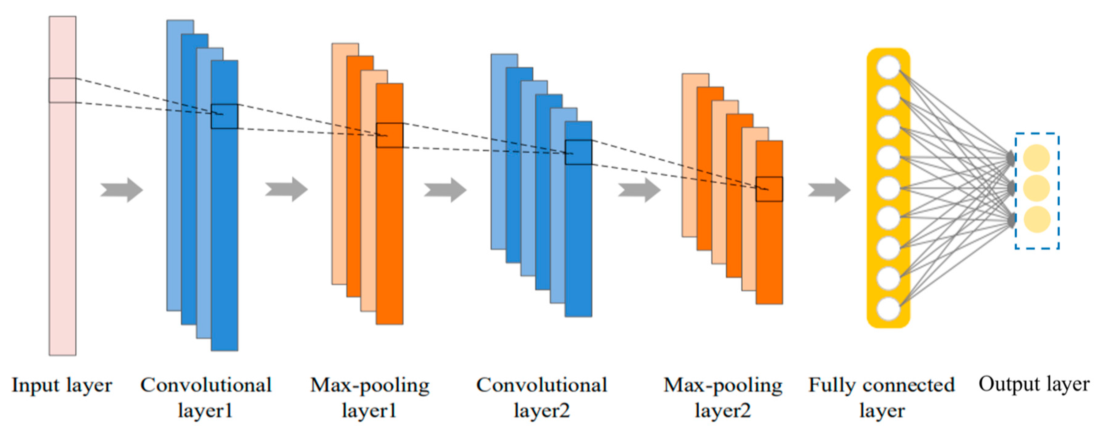
1D CNNs are appropriate for studying one-dimensional data with fixed duration periods. They can automatically extract features from the data and have the characteristics of local connection and shared weights. This significantly decreases the complexity of the state recognition model, conserving computer resources and resulting in more efficient state recognition [40]. The construction of a 1D CNN model is shown in Figure 1.
(1) Convolutional layer
The convolutional layer is critical to feature extraction from cutting data. The exact operation is as follows:
In the formula, is the output of the layer; is the output of the layer; is the convolution kernel corresponding to the layer; is the h-layer bias; is the convolution symbol; and is the activation function.
(2) Pooling layer
The pooling layer’s purpose is to preserve as much information as possible while lowering data dimensions. This study selected the maximum pooling approach, with the specific operation being
In the formula, is the value passed to the corresponding neurons in the layer after the maximum pooling of ; represents the activation value of the neuron in the feature vector of the layer; and denotes the width of the pooling range.
(3) Fully connected layer
The fully connected layer smoothes the multilayer convolution and pooling features in the one-dimensional CNN model into a one-dimensional vector inputs before computing the outputs of each layer’s input pathways as in Equation (19) and the diagnostic results as in Equation (20) in the output layer pathways:
In the formula, is the activation value of the neuron in the layer; is the activation value of the neuron in the lth layer; is the weight between the neuron and the neuron in the layer; and is the bias of all neurons in the layer to the neurons in the layer .
(4) Output layer
The output layer addresses the multi-class problem with a Softmax classifier. The model is represented as follows:
In the formula, is the output result matrix, and and are the weight and bias matrices corresponding to categories.
3. Identification Process of Milling Cutter Wear State Based on Parameter Optimization VMD Multiscale Permutation Entropy and a 1D CNN
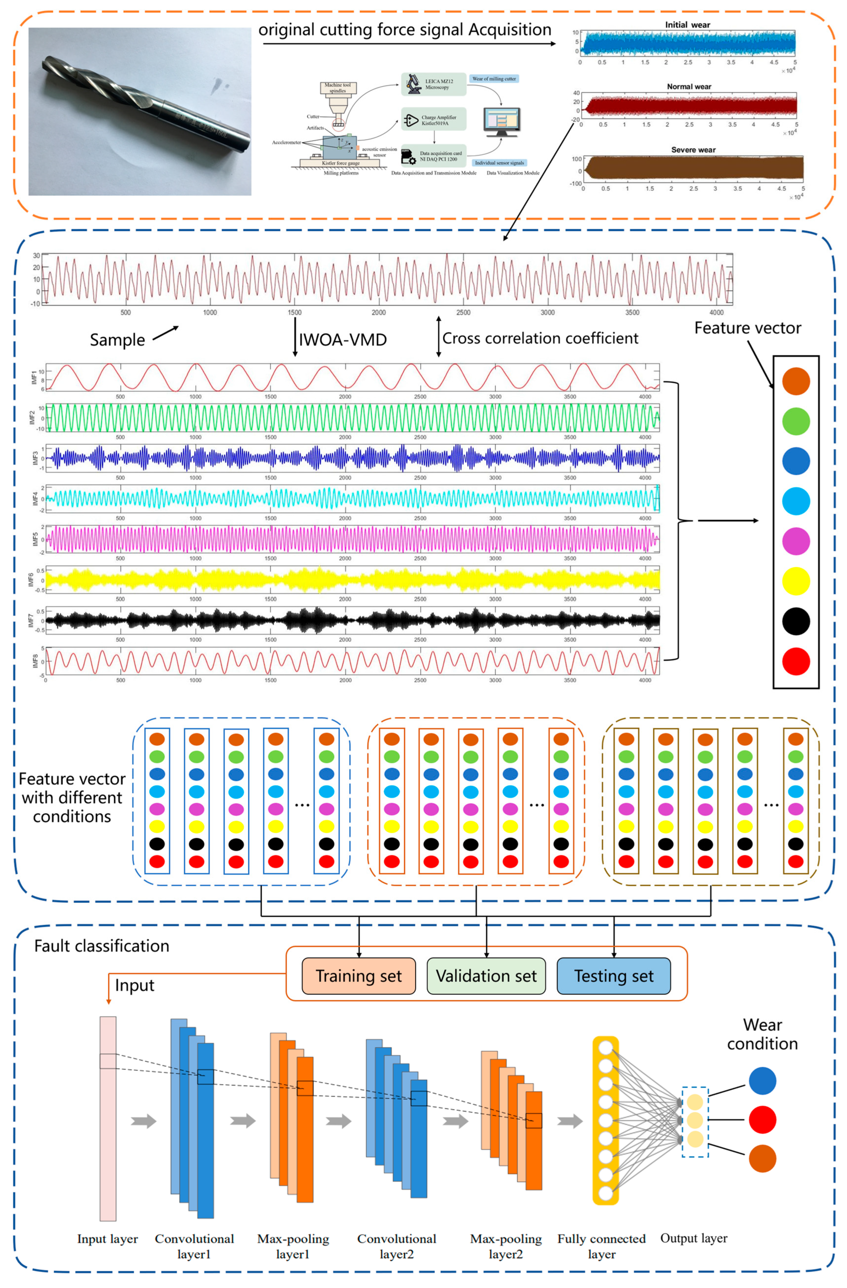
Because the working environment for milling cutter milling is complicated and varied, the cutting force data from on-site sensors is non-smooth, non-linear, and time-varying, among other features. The VMD algorithm, which is robust against noise, is used to decompose the milling vibration signal into multiple IMFs, and the number of interrelationships is used as an index to select the preferred IMFs that are rich in wear feature information, and the MPEs of each IMF are extracted and calculated, as well as the mean value of the multiscale arrangement entropy of each modal. A feature matrix is created using the average Multiscale Permutation Entropy of each mode component and put into a one-dimensional CNN model for state detection. The approach for state identification presented in this work is shown in Figure 2. The precise stages for implementation are as follows:
- (1)
- The IWOA approach is used to find VMD parameters, with the least joint correlation coefficient as the optimization aim.
- (2)
- The optimized VMD is used to decompose the cutting force signal into K IMF components.
- (3)
- Equations (12)–(16) are used to compute the IMF’s Multiscale Permutation Entropy and create the feature vector .
- (4)
- The feature vectors are proportionally partitioned into training and testing sets. A one-dimensional CNN is used to identify the milling tool’s wear state, and the recognition results are then produced.
4. Experimental Examples
4.1. Tool Wear Experiment
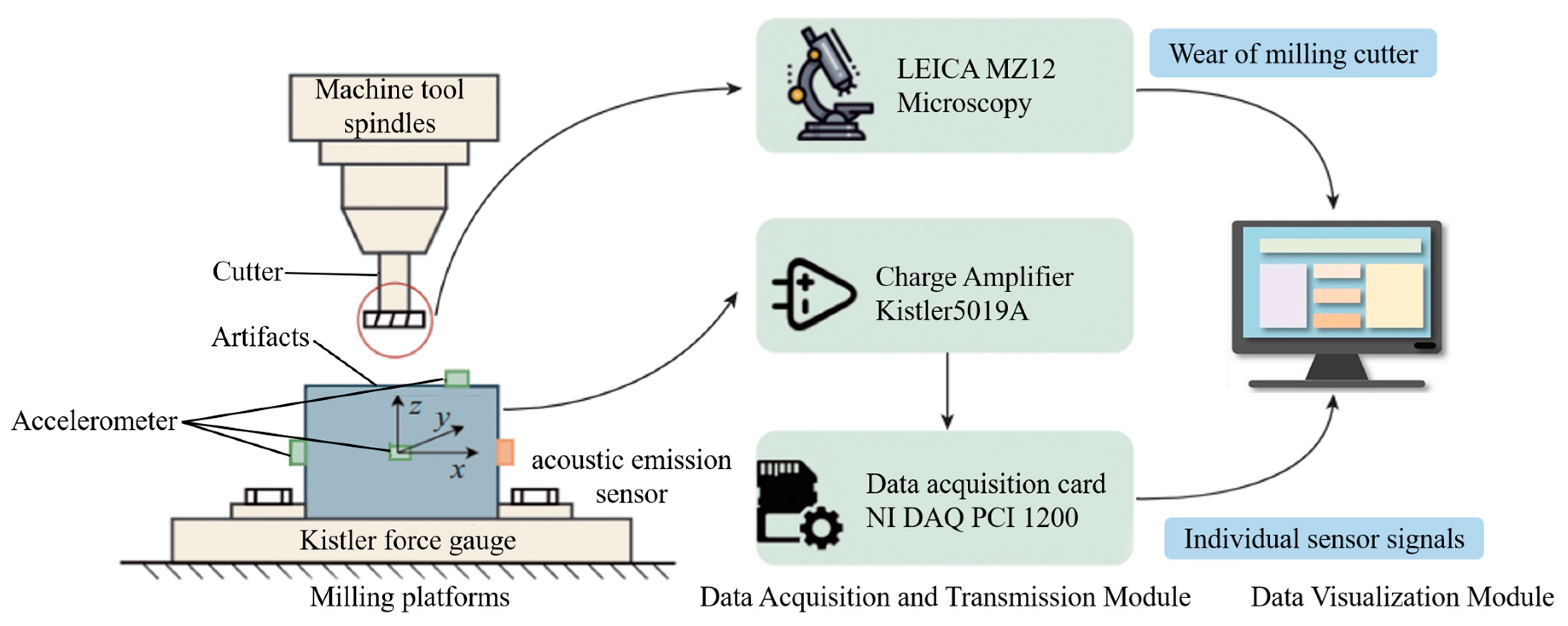
This research demonstrates the technique proposed in this paper by utilizing the public dataset from the 2010 data contest conducted by the PHM Society in the United States [41]. The experimental setup included a Röders-Tech RFM760 high-speed CNC milling machine and a tri-blade hard alloy ball-head vertical milling cutter. The cutting material is stainless steel (HRC52). Figure 3 depicts the equipment platform design, and Table 1 lists the experimental machining settings.
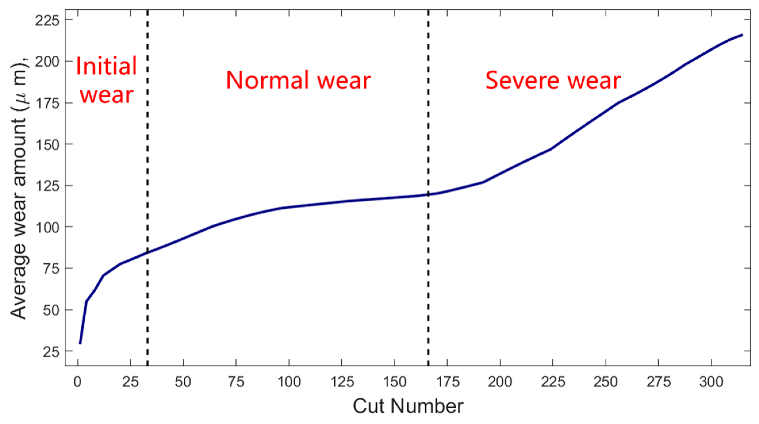
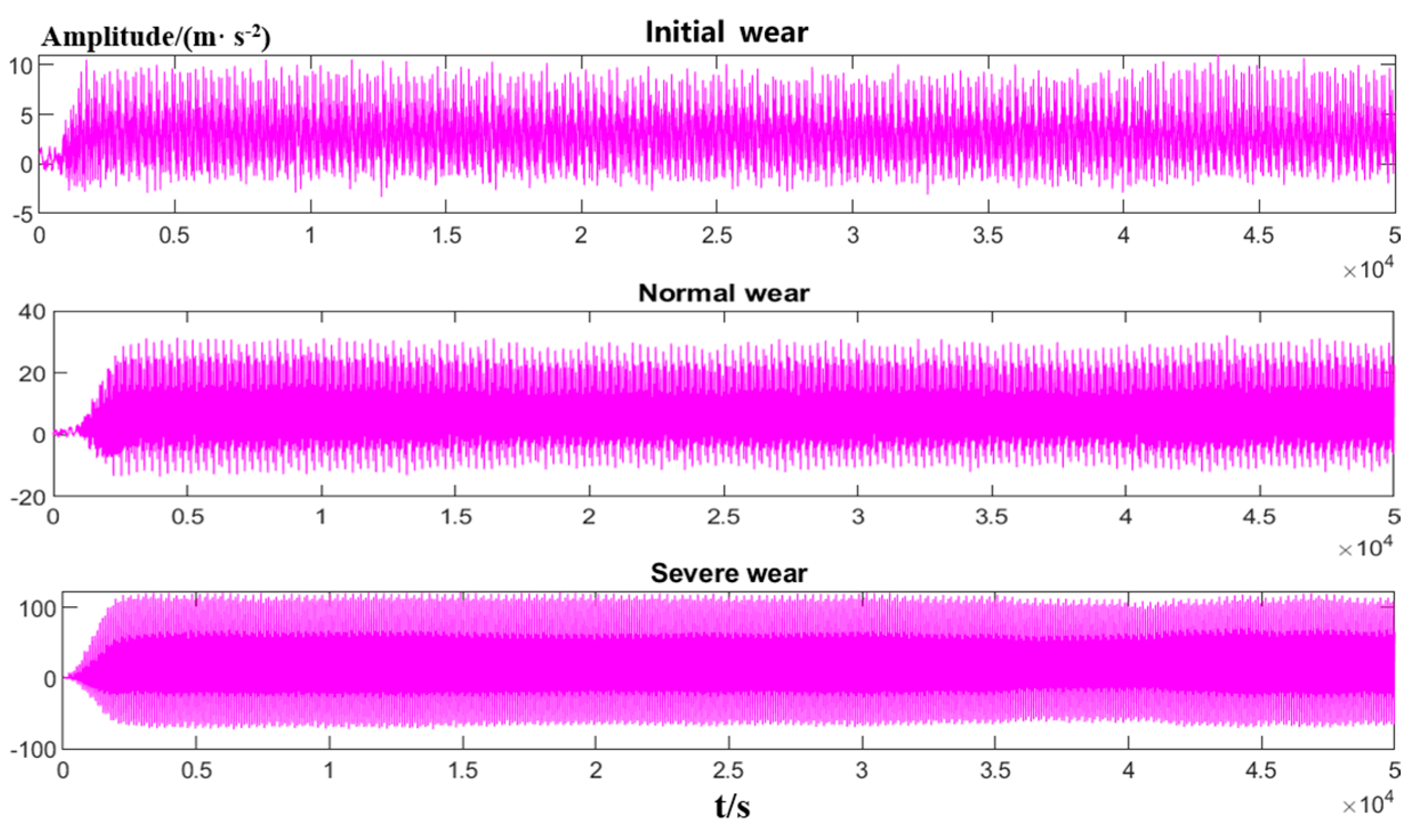
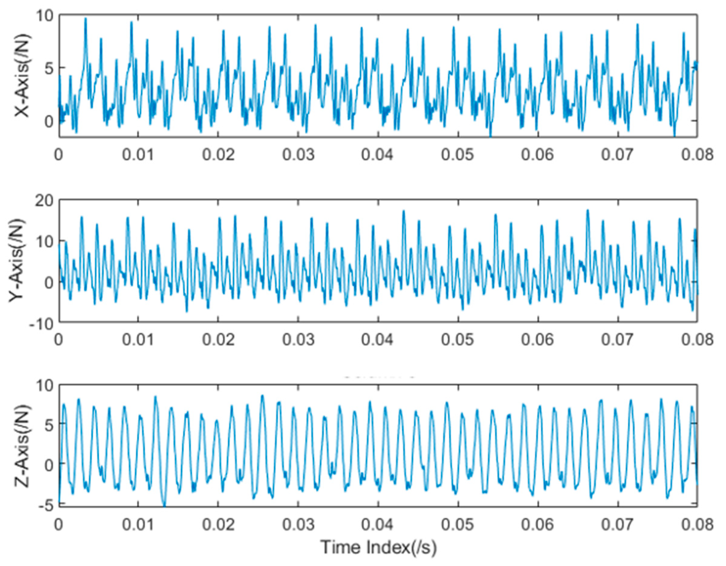
The milling parameters were the same for each tool journey, and the machining workpiece was chosen as square, so the time interval between each tool travel was equal, and the duration of the tool machining may have been simply substituted by the number of tool travels. An NI data card was used to capture acoustic emission, vibration, and cutting force information during the milling operation. The sampling frequency was 50 kHz. At the end of each walk, the rear face wear of the milling cutter was measured and recorded using a Leica MZ12 microscope. The dataset comprised machining data from six different milling cutters (designated C1 through C6) across their full life cycle, with 315 tool walks recorded for each test. In this study, the cutting force signals (x, y, and z) from the C6 milling cutter test dataset were analyzed to create a CNN milling cutter wear state detection model. Figure 4 depicts the mean degradation trajectory for the trio of cutting edges on the C6 milling cutter. In considering the pragmatic conditions of the milling operation, the tool’s initial wear stage was determined to be the first 33 trips; the tool’s normal wear stage was from the 34th to the 166th trip; and the tool entered the severe wear stage on the 167th trip (Figure 5). And the time-frequency plots of the set of multivariate cutting forces in the initial wear state are presented in Figure 6.
4.2. Signal Analysis of Milling Cutter Wear Cutting Force
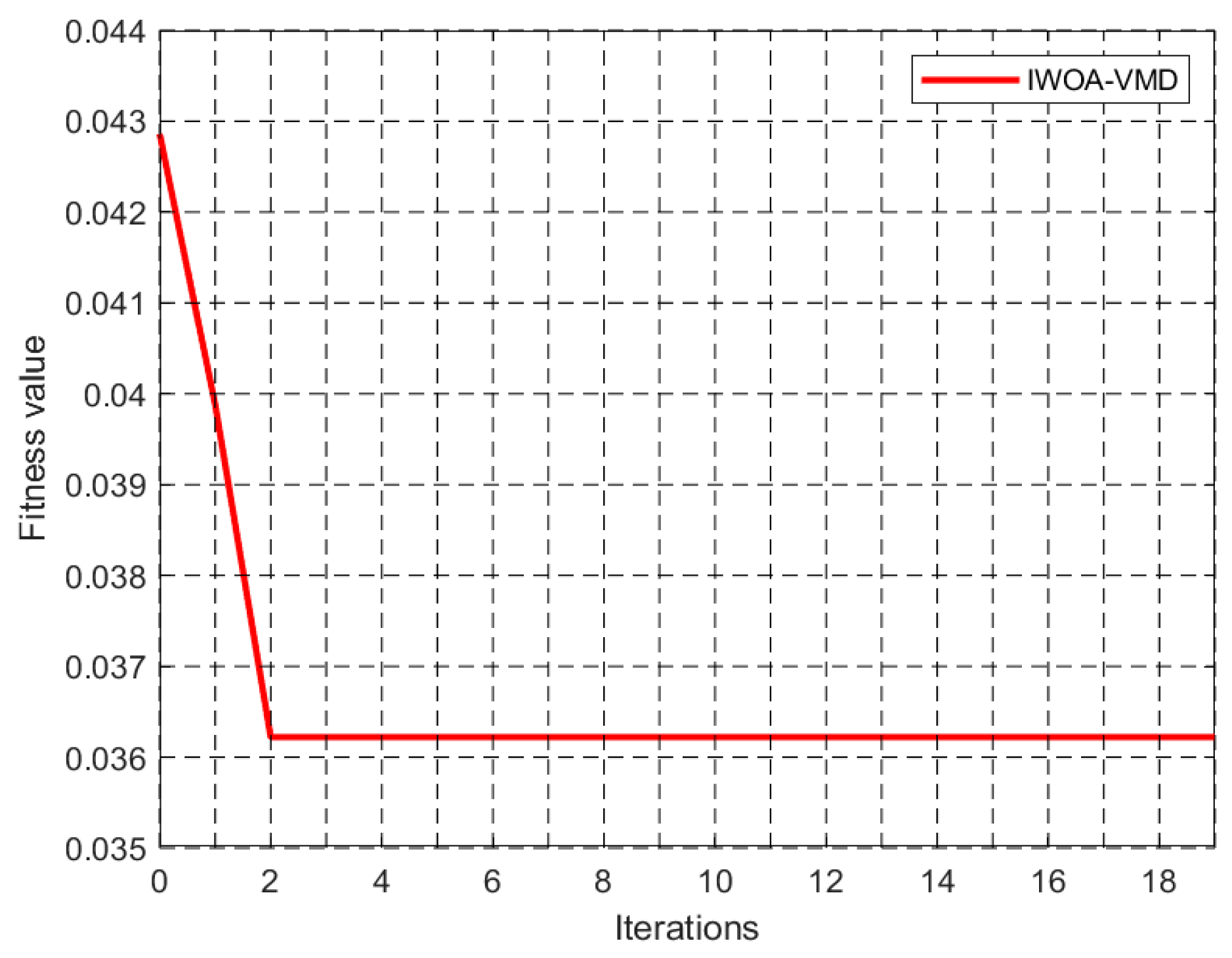
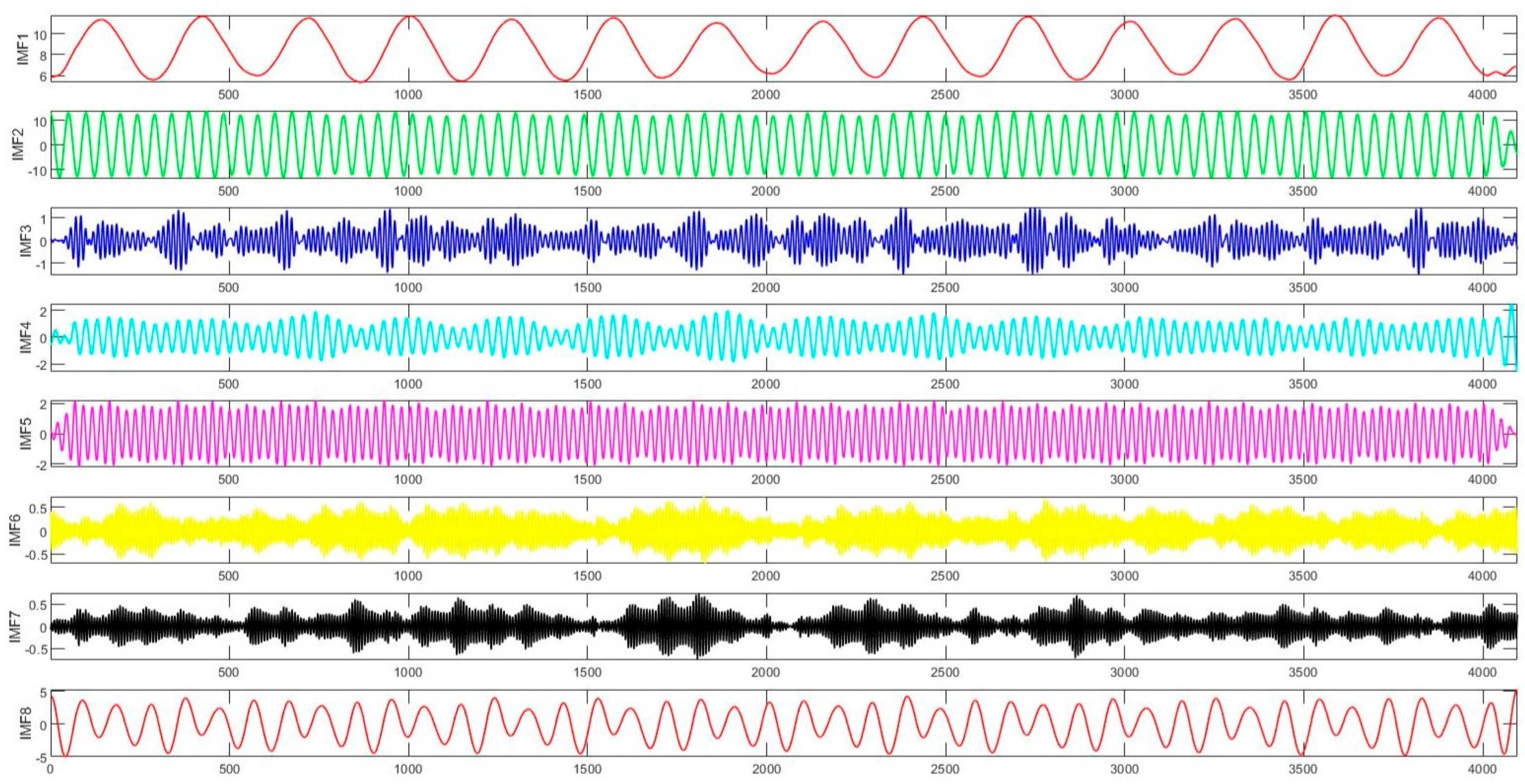
To address difficulties with the WOA algorithm, such as sluggish convergence and sensitivity to local optima, the elite inverse learning method and golden sine algorithm were implemented. The elite reverse learning technique was used to enhance variability within the starting population, and the golden sine algorithm was used to improve the whale’s spiral upward predation, resulting in the IWOA, which improved the algorithm’s speed of convergence and search capabilities. The IWOA algorithm’s population size was set to 50, and it was programmed to iterate a maximum of 20 times. The mode count was , and the penalization coefficient was . Using the signal of the cutting force in the x-direction during the normal wear phase of the milling cutter as a case study, and at the same time, to mitigate the influence of the tool wear condition at the beginning and end of the cutting process, this study employed a sample dataset consisting of 4096 data points for each cutting cycle, ranging from 60,001 to 64,096. The ideal curve was determined through iterative optimization, as seen in Figure 7. The chart shows that the adaptation value is 0.03622 after the second iteration, when it hits a minimum value, and the succeeding iterations converge. The findings demonstrate that the IWOA method achieves quick convergence in VMD parameter optimization. The best VMD parameter, as determined using the IWOA method, is [8,1680.019]. Figure 8 shows the waveform diagrams of each IMF component produced through the IWOA-VMD.
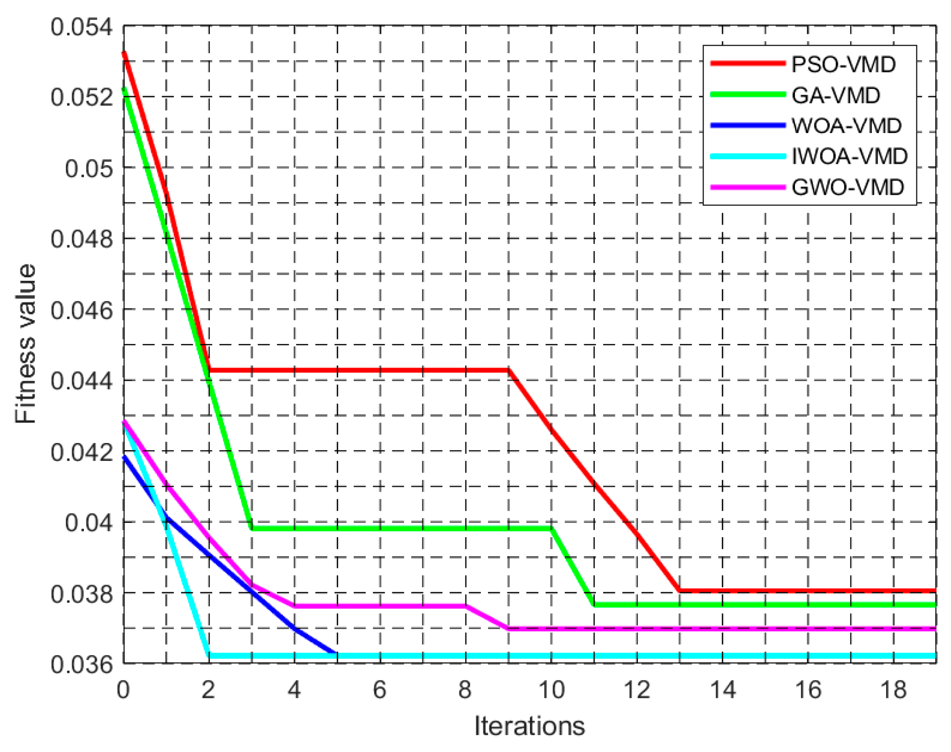
This research demonstrates the superiority of the IWOA method in optimizing VMD parameters, with the combined correlation coefficient as the aim for optimization. Identical settings for the population count and maximum iteration limit were set. The PSO, GA, GWO, and WOA algorithms were employed to repeatedly optimize the VMD parameters, and the resulting curves are presented in Figure 8. According to Figure 9, the PSO method, GA algorithm, GWO algorithm, and WOA algorithm all reached convergence after the 13th, 11th, 9th, and 5th iterations with fitness values of 0.03805, 0.03766, 0.03698, and 0.03622, respectively. As shown in Figure 9, the IWOA algorithm outperforms other algorithms in terms of optimization speed and global search capability, establishing its superiority in optimizing VMD parameters. It also demonstrates the effectiveness of incorporating the elite backward learning strategy and the golden sine algorithm into the IWOA.
4.3. MPE-Based Milling Cutter Wear State Feature Extraction
To improve the signal accuracy, a correlation analysis was performed to evaluate the correlation coefficients between the eight IMF components obtained through VMD and the original signal. Spurious components with interrelationships less than 0.1 were removed. The signal was then reconstructed using the residual IMFs with the highest mutual correlations. As shown in Table 2, the interrelationship numbers of IMF3, IMF4, IMF6, and IMF7 are less than 0.1. Therefore, after deleting the four false categories that were less than 0.1, the original signal was rebuilt using the residual IMFs.
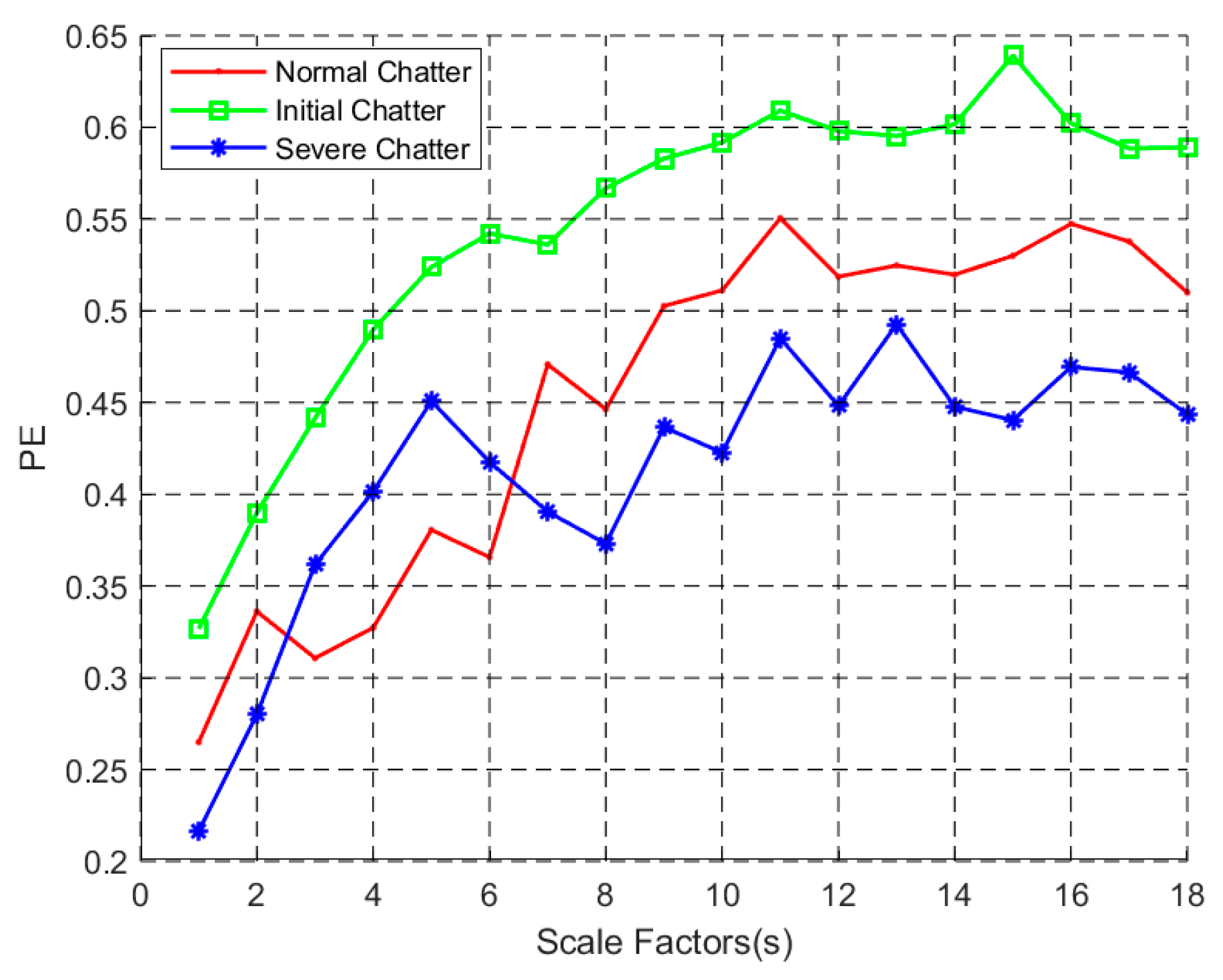
Before computing the MPE of each IMF, the following parameters must be defined: the embedding’s dimensionality, the delay duration, and the scaling factor. According to the research, the optimal dimensionality for embeddings is between three and seven. If the value is insufficiently tiny, the MPE will be unable to accurately depict signal dynamic mutations; if the value is insufficiently great, the time series will become homogenized and ineffective at catching minute changes in the time series data [36]. Following the investigation, we chose 6 as the embedding dimension and 1 as the delay time . There is presently no obvious foundation for selecting scale factors. As a result, in order to discover the appropriate scaling factor, this study examined the change in MPE with scale factor , as shown in Figure 10.
As shown in Figure 10, although three milling cutter wear states may be recognized (i.e., single-scale PE), they are easily confused since their entropy values are quite near to other scale variables. At the same time, it can be seen that the entropy value of the somewhat worn state is the largest, while the entropy value of the severely worn state is the lowest, resulting in an inability to accurately depict the milling cutter’s wear process. This demonstrates that for MPE (that is, when ), especially when the scale factor is present, the MPE increases from stable to serious during the chatter development process, a dynamic process effectively reflecting chatter formation. When , the differences between the three processing conditions are most obvious. As a result, we could select MPE as the best scale factor for determining the milling tool’s attrition status.
4.4. Performance Comparison
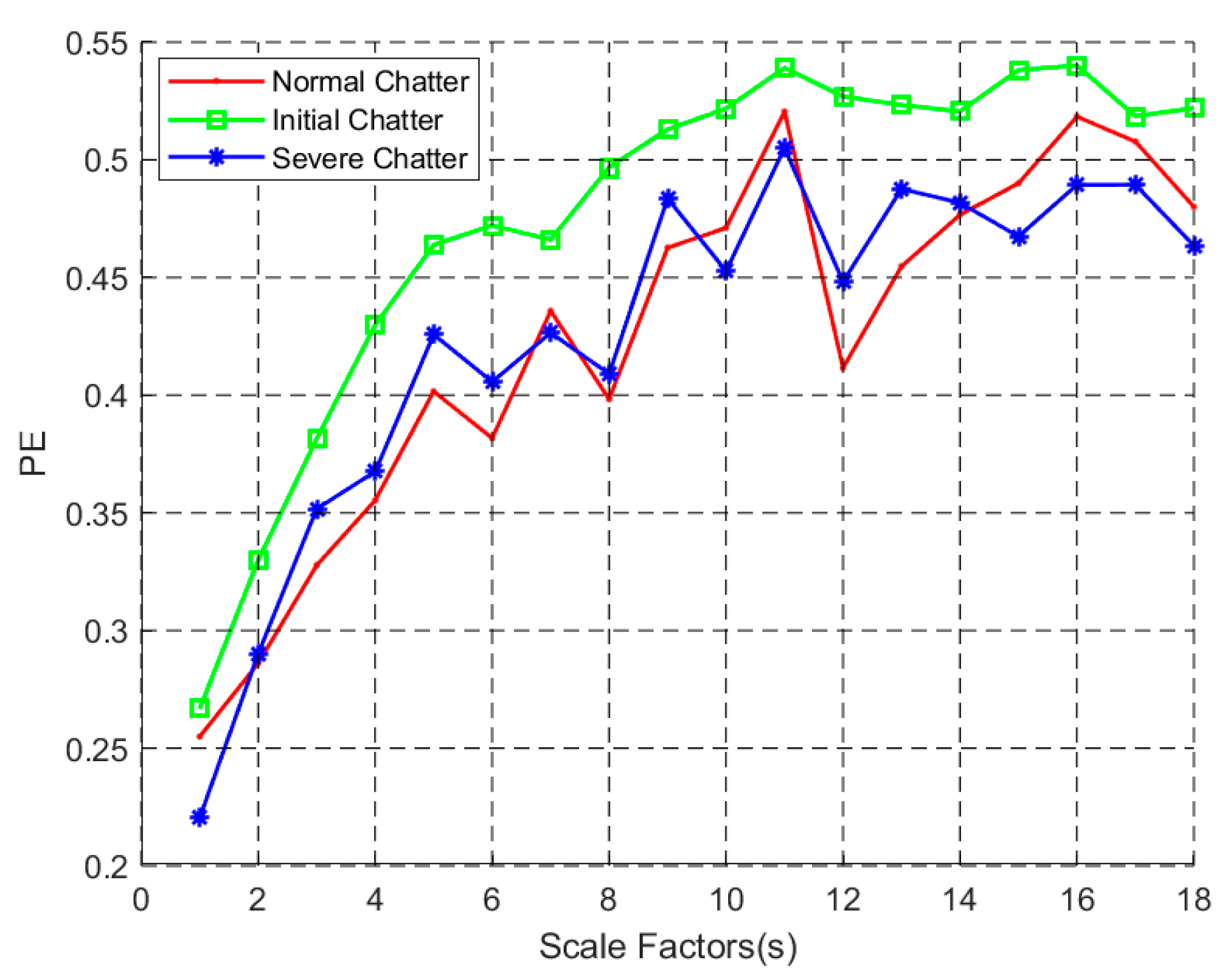
The superiority of this method was demonstrated through a comparative study on the original signal’s MPE values. Figure 11 depicts the fluctuation in MPE of the original signal with the scaling factor. The graph clearly shows that the MPE values for the three wear states are surprisingly similar, making it difficult to discriminate between them based just on MPE values. The cause for this is the substantial noise inherent in the initial cutting force signal, which interferes with milling cutter wear status detection.
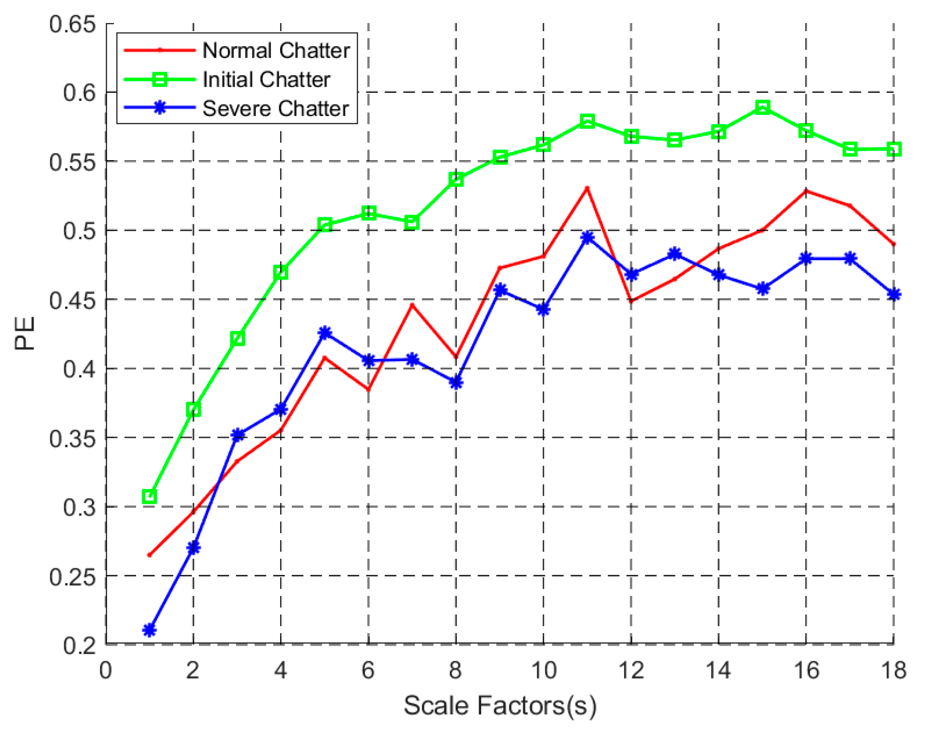
To demonstrate the advantages of the technique used in this study, the algorithm was compared to the unoptimized VMD. When utilizing unoptimized VMD, K and were determined through the IWOA’s random initialization procedure. Table 3 shows the signal decomposition parameters in three states, together with their minimal joint correlation coefficients. Figure 12 demonstrates the extraction of MPE values at different scales using the control variable method. The unoptimized VMD could discriminate between normal and the other two wear states, but not between minor and severe wear states. Figure 12 shows that the unoptimized VMD-MPE fails to recognize the milling tool’s wear state as efficiently as the AVMD-MPE.
The comparison analysis above demonstrates that parameters K and have a significant impact on the efficacy of VMD decomposition. If K and are not appropriate values, no matter how the scale factor is chosen, it will be impossible to discern the three milling cutter wear stages using the VMD-MPE approach.
4.5. Identification Results of Milling Cutter Wear State
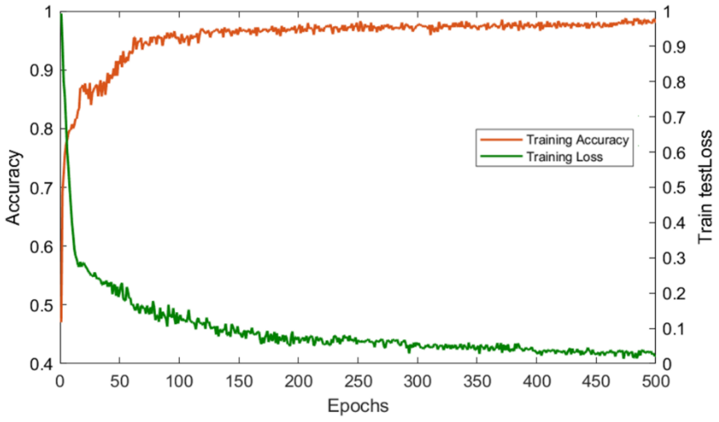
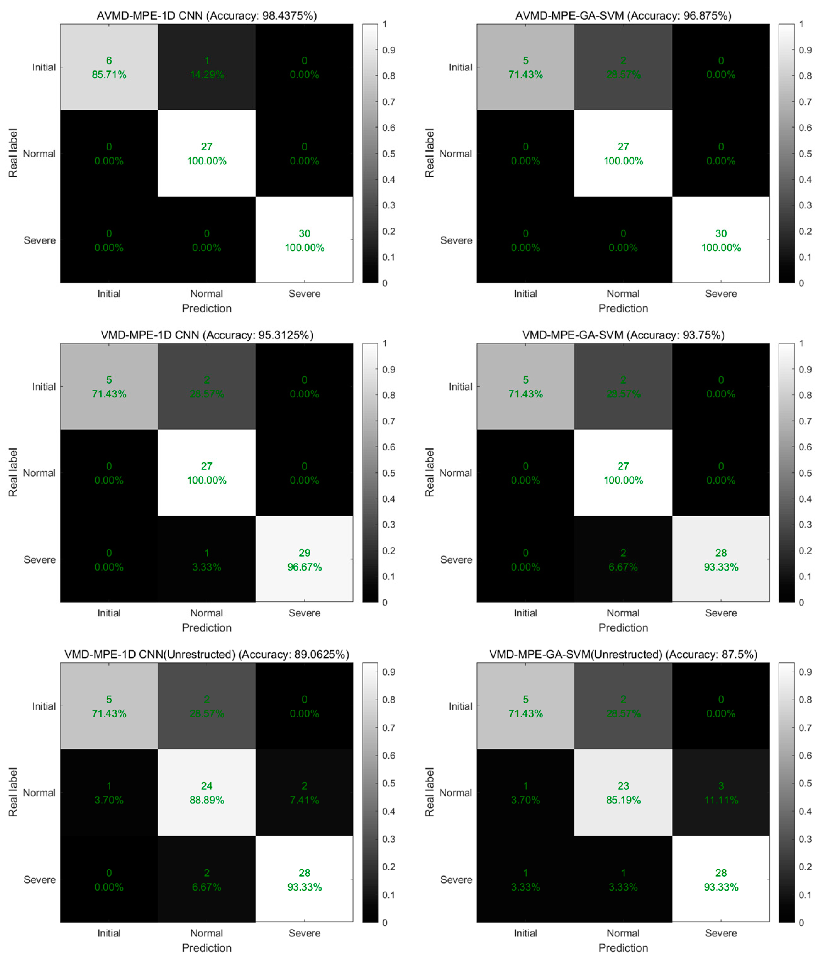
This research analyzed the multivariable cutting force signal of C6. On this basis, a feature vector was generated from the MPE value of the multivariable cutting force signal. According to the earlier discussion on the categorization of the C6 milling cutter’s wear condition, the datasets for training, validation, and testing were randomly distributed in proportions of 0.6:0.2:0.2 for each wear scenario. Multiple experiments were performed to adjust the 1D CNN model to the study’s needs. The final architecture of the 1D CNN model consisted of two convolutional layers, two max-pooling layers, two batch normalization layers, a flattened layer, a dropout layer, and two fully connected layers. The ReLU activation function was used to speed up the model’s convergence, and a dropout layer was added after the fully linked layers to prevent overfitting. During training, each neuron in the buried layer’s output was negated with a probability of p = 0.5, eliminating reciprocal dependencies between neurons [42]. The best parameters for the 1D CNN model were determined through numerous trials. T Adam was chosen as the optimizer, with a fixed learning rate of 0.0001 and a batch size of 12. Tensorflow was used to build a one-dimensional CNN model, and its recognition accuracy is shown in Figure 13. To demonstrate the advantages of the approach presented in this work, it was compared against AVMD-MPE-GA-SVM, VMD-MPEE-IDCNN, VMD-MPE-GA-SVM, VMD-MPE-1DCNN (unreconstructed), and VMD-MPE-GA-SVM (unreconstructed). As shown in Figure 14, the recognition accuracies of the AVMD and 1D CNN methods for three wear states of the milling cutter were 98.4375% (63/64), allowing for the exact determination of the milling cutter’s wear condition. The recognition accuracy of the AVMD + GA-SVM technique was 96.875% (62/64), owing to the superior recognition performance of the deep learning model over the machine learning model.
The accuracies of the VMD + 1D CNN and VMD + GA-SVM techniques were 95.3125% (61/64) and 93.75% (60/64), respectively. This might be because the VMD parameters and are not ideal, resulting in a decomposition effect that differs greatly from the first group. In the final group, the signal with a high correlation coefficient with the original signal was not optimized after unoptimized VMD. The recognition performance of this group is clearly lower than that of the first two groups. This is because, following the unoptimized VMD, not all of the produced IMFs were significantly associated with the original signal, resulting in the group’s worst decomposition effect. The VMD + 1D CNN (unreconstructed) and VMD + GA-SVM (unreconstructed) approaches exhibited accuracies of only 89.0625% (57/64) and 87.5 (56/64), respectively. Therefore, by comparing the VMD + 1D CNN approach to the classic machine learning classification model and other algorithms, its efficacy and practicability are proven, and the effective classification of the wear condition of the milling cutter is achieved.
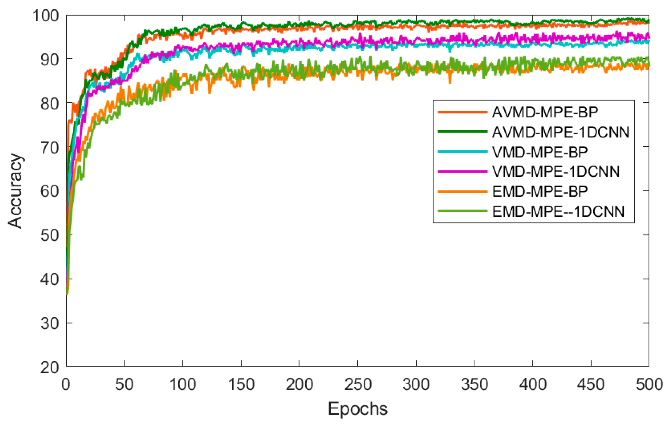
Figure 15 shows the connection between the accuracies and iteration counts for EMD-MPE-BP, EMD-MPE-1D CNN, VMD-MPE-BP, VMD-MPE-1D CNN, AVMD-MPE-BP, and AVMD-MPE-1D CNN, which provides further support for the benefits of the technique used in this research. It is clear that the BP and 1D CNN networks achieve excellent accuracy after around 150 iterations, with the following iterations beginning to settle. After 150 iterations, the recognition rate of the 1D CNN is essentially steady, demonstrating that the ID CNN may increase the recognition accuracy and reflecting its superiority.
5. Conclusions
A technique was developed to address the difficulty in monitoring the wear status of milling cutters in CNC machine tools, which is caused by the non-linear and non-stationary characteristics of the cutting force signal. This technique is based on feature extraction via parameter-optimized VMD-MPE and includes a 1D CNN recognition model for detecting milling cutter wear. This approach is used as a reference for recognizing the condition of milling cutters in CNC machine tools, which helps to improve the precision and efficiency of the thin-walled component production process. The main conclusions of the study are as follows:
- (1)
- The suggested IWOA-VMD technique can successfully evaluate the milling cutter’s cutting force signal and has several benefits.
- (2)
- Multiscale Permutation Entropy may be used to efficiently derive the wear characteristics of a CNC milling cutter.
- (3)
- A one-dimensional CNN used as the input model for feature vectors outperforms the comparable models, illustrating the proposed approach’s major benefits.
- (4)
- Using this strategy to identify milling cutter wear situations results in a detection rate of up to 98.4375%, which is superior to those of comparable methods.
- (5)
- Future work includes identifying milling cutter wear conditions under variable speed conditions, selecting multidimensional feature vectors as input vectors for the identification model, and recognizing milling cutter wear conditions based on imbalanced or multi-channel data.
Author Contributions
The design, verification, and writing of the milling cutter wear state recognition model in this study were completed by the author X.S. The research ideas and full-text guidance were provided by Z.R. and B.D. The modification of the full-text details and the improvement of the format were completed by the authors Q.H. and X.Y. All authors have read and agreed to the published version of the manuscript.
Funding
This research was funded by the Key Research and Development Program of Hubei Province (ID: 2022BAA059).
Data Availability Statement
Experimental data were obtained from the Prognostics and Health Management Society 2010 PHM Society Conference Data Challenge. The resource can be found in the corresponding reference.
Conflicts of Interest
The authors declare no conflict of interest.
References
- Wei, X.; Liu, X.; Yue, C.; Wang, L.; Liang, S.Y.; Qin, Y. Tool Wear State Recognition Based on Feature Selection Method with Whitening Variational Mode Decomposition. Robot. Comput. Integr. Manuf. 2022, 77, 102344. [Google Scholar] [CrossRef]
- Nasir, V.; Sassani, F. A Review on Deep Learning in Machining and Tool Monitoring: Methods, Opportunities, and Challenges. Int. J. Adv. Manuf. Technol. 2021, 115, 2683–2709. [Google Scholar] [CrossRef]
- Dai, Y.; Zhu, K. A Machine Vision System for Micro-Milling Tool Condition Monitoring. Precis. Eng. J. Int. Soc. Precis. Eng. Nanotechnol. 2018, 52, 183–191. [Google Scholar] [CrossRef]
- Nair, U.; Krishna, B.M.; Namboothiri, V.N.N.; Nampoori, V.P.N. Permutation Entropy Based Real-Time Chatter Detection Using Audio Signal in Turning Process. Int. J. Adv. Manuf. Technol. 2009, 46, 61–68. [Google Scholar] [CrossRef]
- Niroomand, M.R.; Forouzan, M.R.; Heidari, A. Experimental Analysis of Vibration and Sound in Order to Investigate Chatter Phenomenon in Cold Strip Rolling. Int. J. Adv. Manuf. Technol. 2019, 100, 673–682. [Google Scholar] [CrossRef]
- Dong, X.; Zhang, W. Chatter Identification in Milling of the Thin-Walled Part Based on Complexity Index. Int. J. Adv. Manuf. Technol. 2017, 91, 3327–3337. [Google Scholar] [CrossRef]
- Zhu, L.; Liu, C.; Ju, C.; Guo, M. Vibration Recognition for Peripheral Milling Thin-Walled Workpieces Using Sample Entropy and Energy Entropy. Int. J. Adv. Manuf. Technol. 2020, 108, 3251–3266. [Google Scholar] [CrossRef]
- Ji, Y.; Wang, X.; Liu, Z.; Yan, Z.; Jiao, L.; Wang, D.; Wang, J. Eemd-Based Online Milling Chatter Detection by Fractal Dimension and Power Spectral Entropy (Vol 92, Pg 1185, 2017). Int. J. Adv. Manuf. Technol. 2020, 111, 2401–2402. [Google Scholar] [CrossRef]
- Liu, J.; Hu, Y.; Wu, B.; Jin, C. A Hybrid Health Condition Monitoring Method in Milling Operations. Int. J. Adv. Manuf. Technol. 2017, 92, 2069–2080. [Google Scholar] [CrossRef]
- Liu, Y.; Wang, X.; Lin, J.; Zhao, W. Early Chatter Detection in Gear Grinding Process Using Servo Feed Motor Current. Int. J. Adv. Manuf. Technol. 2016, 83, 1801–1810. [Google Scholar] [CrossRef]
- Li, Y.; Zhou, S.; Lin, J.; Wang, X. Regenerative Chatter Identification in Grinding Using Instantaneous Nonlinearity Indicator of Servomotor Current Signal. Int. J. Adv. Manuf. Technol. 2017, 89, 779–790. [Google Scholar] [CrossRef]
- Zhu, L.; Liu, C. Recent Progress of Chatter Prediction, Detection and Suppression in Milling. Mech. Syst. Signal Process. 2020, 143, 106840. [Google Scholar] [CrossRef]
- Chen, Y.; Li, H.; Jing, X.; Hou, L.; Bu, X. Intelligent Chatter Detection Using Image Features and Support Vector Machine. Int. J. Adv. Manuf. Technol. 2019, 102, 1433–1442. [Google Scholar] [CrossRef]
- Lei, N.; Soshi, M. Vision-Based System for Chatter Identification and Process Optimization in High-Speed Milling. Int. J. Adv. Manuf. Technol. 2017, 89, 2757–2769. [Google Scholar] [CrossRef]
- Benkedjouh, T.; Zerhouni, N.; Rechak, S. Tool Wear Condition Monitoring Based on Continuous Wavelet Transform and Blind Source Separation. Int. J. Adv. Manuf. Technol. 2018, 97, 3311–3323. [Google Scholar] [CrossRef]
- Laddada, S.; Si-Chaib, M.O.; Benkedjouh, T.; Drai, R. Tool Wear Condition Monitoring Based on Wavelet Transform and Improved Extreme Learning Machine. Proc. Inst. Mech. Eng. Part C J. Mech. Eng. Sci. 2020, 234, 1057–1068. [Google Scholar] [CrossRef]
- Babouri, M.K.; Ouelaa, N.; Djebala, A. Experimental Study of Tool Life Transition and Wear Monitoring in Turning Operation Using a Hybrid Method Based on Wavelet Multi-Resolution Analysis and Empirical Mode Decomposition. Int. J. Adv. Manuf. Technol. 2016, 82, 2017–2028. [Google Scholar] [CrossRef]
- Yang, K.; Wang, G.; Dong, Y.; Zhang, Q.; Sang, L. Early Chatter Identification Based on an Optimized Variational Mode Decomposition. Mech. Syst. Signal Process. 2019, 115, 238–254. [Google Scholar] [CrossRef]
- Lei, Y.; Lin, J.; He, Z.; Zuo, M.J. A Review on Empirical Mode Decomposition in Fault Diagnosis of Rotating Machinery. Mech. Syst. Signal Process. 2013, 35, 108–126. [Google Scholar] [CrossRef]
- Dragomiretskiy, K.; Zosso, D. Variational Mode Decomposition. IEEE Trans. Signal Process. 2014, 62, 531–544. [Google Scholar] [CrossRef]
- Liu, C.; Zhu, L.; Ni, C. Chatter Detection in Milling Process Based on VMD and Energy Entropy. Mech. Syst. Signal Process. 2018, 105, 169–182. [Google Scholar] [CrossRef]
- Liu, B.; Liu, C.; Zhou, Y.; Wang, D. A Chatter Detection Method in Milling Based on Gray Wolf Optimization VMD and Multi-Entropy Features. Int. J. Adv. Manuf. Technol. 2023, 125, 831–854. [Google Scholar] [CrossRef]
- Paternina, M.R.A.; Tripathy, R.K.; Zamora-Mendez, A.; Dotta, D. Identification of Electromechanical Oscillatory Modes Based on Variational Mode Decomposition. Electr. Power Syst. Res. 2019, 167, 71–85. [Google Scholar] [CrossRef]
- Sharma, M.; Kaur, P. A Comprehensive Analysis of Nature-Inspired Meta-Heuristic Techniques for Feature Selection Problem. Arch. Comput. Methods Eng. 2021, 28, 1103–1127. [Google Scholar] [CrossRef]
- Mirjalili, S.; Lewis, A. The Whale Optimization Algorithm. Adv. Eng. Softw. 2016, 95, 51–67. [Google Scholar] [CrossRef]
- Wang, X.; Si, S.; Li, Y. Multiscale Diversity Entropy: A Novel Dynamical Measure for Fault Diagnosis of Rotating Machinery. IEEE Trans. Ind. Inform. 2021, 17, 5419–5429. [Google Scholar] [CrossRef]
- Richman, J.S.; Moorman, J.R. Physiological Time-Series Analysis Using Approximate Entropy and Sample Entropy. Am. J. Physiol. Heart Circ. Physiol. 2000, 278, H2039–H2049. [Google Scholar] [CrossRef]
- Chen, W.; Wang, Z.; Xie, H.; Yu, W. Characterization of Surface EMG Signal Based on Fuzzy Entropy. IEEE Trans. Neural Syst. Rehabil. Eng. 2007, 15, 266–272. [Google Scholar] [CrossRef]
- Peng, D.; Li, H.; Ou, J.; Wang, Z. Milling Chatter Identification by Optimized Variational Mode Decomposition and Fuzzy Entropy. Int. J. Adv. Manuf. Technol. 2022, 121, 6111–6124. [Google Scholar] [CrossRef]
- Li, Y.; Xu, M.; Wei, Y.; Huang, W. A New Rolling Bearing Fault Diagnosis Method Based on Multiscale Permutation Entropy and Improved Support Vector Machine Based Binary Tree. Measurement 2016, 77, 80–94. [Google Scholar] [CrossRef]
- Li, Y.; Wang, X.; Liu, Z.; Liang, X.; Si, S. The Entropy Algorithm and Its Variants in the Fault Diagnosis of Rotating Machinery: A Review. IEEE Access 2018, 6, 66723–66741. [Google Scholar] [CrossRef]
- Bandt, C.; Pompe, B. Permutation Entropy: A Natural Complexity Measure for Time Series. Phys. Rev. Lett. 2002, 88, 174102. [Google Scholar] [CrossRef]
- Liu, X.; Wang, Z.; Li, M.; Yue, C.; Liang, S.Y.; Wang, L. Feature Extraction of Milling Chatter Based on Optimized Variational Mode Decomposition and Multi-Scale Permutation Entropy. Int. J. Adv. Manuf. Technol. 2021, 114, 2849–2862. [Google Scholar] [CrossRef]
- Yang, D.; Lv, Y.; Yuan, R.; Li, H.; Zhu, W. Robust Fault Diagnosis of Rolling Bearings via Entropy-Weighted Nuisance Attribute Projection and Neural Network under Various Operating Conditions. Struct. Health Monit. An Int. J. 2022, 21, 2890–2909. [Google Scholar] [CrossRef]
- Yang, X.; Yuan, R.; Lv, Y.; Li, L.; Song, H. A Novel Multivariate Cutting Force-Based Tool Wear Monitoring Method Using One-Dimensional Convolutional Neural Network. Sensors 2022, 22, 8343. [Google Scholar] [CrossRef]
- Kuo, P.-H.; Lin, C.-Y.; Luan, P.-C.; Yau, H.-T. Dense-Block Structured Convolutional Neural Network-Based Analytical Prediction System of Cutting Tool Wear. IEEE Sens. J. 2022, 22, 20257–20267. [Google Scholar] [CrossRef]
- Wang, W.; Guo, S.; Zhao, S.; Lu, Z.; Xing, Z.; Jing, Z.; Wei, Z.; Wang, Y. Intelligent Fault Diagnosis Method Based on Vmd-Hilbert Spectrum and Shufflenet-V2: Application to the Gears in a Mine Scraper Conveyor Gearbox. Sensors 2023, 23, 4951. [Google Scholar] [CrossRef]
- Tubishat, M.; Abushariah, M.A.M.; Idris, N.; Aljarah, I. Improved Whale Optimization Algorithm for Feature Selection in Arabic Sentiment Analysis. Appl. Intell. 2019, 49, 1688–1707. [Google Scholar] [CrossRef]
- Tanyildizi, E.; Demir, G. Golden Sine Algorithm: A Novel Math-Inspired Algorithm. Adv. Electr. Comput. Eng. 2017, 17, 71–78. [Google Scholar] [CrossRef]
- Peng, D.; Liu, Z.; Wang, H.; Qin, Y.; Jia, L. A Novel Deeper One-Dimensional Cnn with Residual Learning for Fault Diagnosis of Wheelset Bearings in High-Speed Trains. IEEE Access 2019, 7, 10278–10293. [Google Scholar] [CrossRef]
- PHM Society, 2010 Phm Society Conference Data Challenge. 2010. Available online: https://www.kaggle.com/datasets/tobbyrui/phm2010 (accessed on 25 December 2022).
- Wu, X.; Liu, Y.; Zhou, X.; Mou, A. Automatic Identification of Tool Wear Based on Convolutional Neural Network in Face Milling Process. Sensors 2019, 19, 3817. [Google Scholar] [CrossRef] [PubMed]
Figure 1.
Structure of a one-dimensional CNN model.

Figure 2.
State recognition process.

Figure 3.
Architecture of the experimental device for tool wear monitoring.

Figure 4.
Change curve of average wear of C6 milling cutter.

Figure 5.
Cutting force signals of milling cutter in three states.

Figure 6.
Time−frequency diagram of multivariate cutting force signals in the initial state.

Figure 7.
IWOA-optimized VMD parameter iteration profile.

Figure 8.
IWOA−VMD decomposition result plot.

Figure 9.
Comparison diagram of VMD parameters optimized using multiple algorithms.

Figure 10.
MPE changes with scale factor after signal reconstruction using the IWOA-VMD method.

Figure 11.
Variation in the MPE of the original signal with the scaling factor.

Figure 12.
Effect of non-optimized VMD on the change in MPE of the reconstructed signal with scaling factor.
Figure 12.
Effect of non-optimized VMD on the change in MPE of the reconstructed signal with scaling factor.

Figure 13.
1D CNN state recognition accuracy curve.

Figure 14.
Classification confusion matrix of different status identification methods.

Figure 15.
VMD and neural network combination comparison accuracy.


Table 1.
Experimental parameters.
| Spindle Speed/rpm | Feed Speed/(mm/min) | Radial Cutting Depth/mm | Axial Cutting Depth/mm | Milling Method |
|---|---|---|---|---|
| 10,400 | 1555 | 0.125 | 0.2 | climb milling |
Table 2.
Number of correlations between each modal component and the corresponding original signal.
| IMF | IMF1 | IMF2 | IMF3 | IMF4 | IMF5 | IMF6 | IMF7 | IMF8 |
|---|---|---|---|---|---|---|---|---|
| correlation coefficient | 0.2788 | 0.9181 | 0.0716 | 0.0381 | 0.1598 | 0.034 | 0.0255 | 0.3085 |
Table 3.
Random initialization parameters and joint correlation coefficient.
| Cutting State | K | Joint Correlation Coefficient | |
|---|---|---|---|
| Initial chatter | 7 | 2654 | 0.0432 |
| Normal chatter | 6 | 4378 | 0.0429 |
| Severe chatter | 7 | 921 | 0.0435 |
Disclaimer/Publisher’s Note: The statements, opinions and data contained in all publications are solely those of the individual author(s) and contributor(s) and not of MDPI and/or the editor(s). MDPI and/or the editor(s) disclaim responsibility for any injury to people or property resulting from any ideas, methods, instructions or products referred to in the content. |
© 2024 by the authors. Licensee MDPI, Basel, Switzerland. This article is an open access article distributed under the terms and conditions of the Creative Commons Attribution (CC BY) license (https://creativecommons.org/licenses/by/4.0/).
Share and Cite
MDPI and ACS Style
Shui, X.; Rong, Z.; Dan, B.; He, Q.; Yang, X. Tool Wear State Identification Based on the IWOA-VMD Feature Selection Method. Machines 2024, 12, 184. https://doi.org/10.3390/machines12030184
AMA Style
Shui X, Rong Z, Dan B, He Q, Yang X. Tool Wear State Identification Based on the IWOA-VMD Feature Selection Method. Machines. 2024; 12(3):184. https://doi.org/10.3390/machines12030184
Chicago/Turabian StyleShui, Xing, Zhijun Rong, Binbin Dan, Qiangjian He, and Xin Yang. 2024. "Tool Wear State Identification Based on the IWOA-VMD Feature Selection Method" Machines 12, no. 3: 184. https://doi.org/10.3390/machines12030184
Note that from the first issue of 2016, this journal uses article numbers instead of page numbers. See further details here.