
Numerical Investigation of Background Noise in a Circulating Water Tunnel

School of Naval Architecture & Ocean Engineering, Huazhong University of Science and Technology, Wuhan 430074, China
*
Author to whom correspondence should be addressed.
Machines 2023, 11(8), 839; https://doi.org/10.3390/machines11080839
Submission received: 30 June 2023
/
Revised: 7 August 2023
/
Accepted: 10 August 2023
/
Published: 18 August 2023
(This article belongs to the Special Issue Machine Science and Research in HUST: Celebrating the 70th Anniversary of Huazhong University of Science and Technology)
Abstract
:The presence of excessive background noise in hydrodynamic noise experiments conducted in circulating water tunnels can significantly impact the accuracy and reliability of experimental test results. To address this issue, it is crucial to evaluate and optimize the background noise during the design stage. In this research, acoustic field model and fluid–solid coupling numerical calculation model of circulating water tunnels are established. Utilizing the finite element method, we analyze the flow noise and flow-excited noise resulting from wall pressure pulses in the circulating water tunnel. Furthermore, we conduct a noise contribution analysis and explore strategies for structural vibration noise control. The results demonstrate that both flow noise and flow-excited noise decrease with increasing frequency, with flow-excited noise being the primary component of the tunnel’s background noise. The presence of resonant peaks significantly contributes to the elevated flow-excited noise levels. Moreover, enhancing structural stiffness and damping proves less effective in suppressing low-frequency peaks. Additionally, employing sound measurement pods suspended from the side of the test section for noise measurement exhibits a high error rate at low frequencies. This research provides insights into optimizing background noise in water tunnels, thereby informing future enhancements in tunnel design.
1. Introduction
The hydrodynamic performance of underwater vehicles plays a crucial role in their overall functionality, with the hydrodynamic noise level serving as a significant indicator [1]. The circulating water tunnel represents the most established and widely utilized apparatus for conducting hydrodynamic noise tests. However, during such experiments, the flow field in inadequately designed water tunnels is highly turbulent, influenced by the tunnel walls. Consequently, this turbulence generates substantial hydrodynamic background noise, resulting in a low signal-to-noise ratio for the intended research targets [2]. Therefore, it becomes imperative to predict the noise performance of water tunnels during their design and construction phases.
The hydrodynamic background noise in circulating water tunnels arises from a combination of disturbances within the turbulent boundary layer, wall pressure pulses in the flow field, and structural vibrations induced by fluid–solid interaction. The velocity perturbations and wall pressure pulsations within the turbulent boundary layer can be regarded as the equivalent of quadrupole and dipole sources, respectively. These components collectively contribute to the flow noise, with the dipole source formed by the wall pressure pulses constituting the major portion. Furthermore, the interaction between the fluid and the elastic structure leads to structural vibrations, which generate flow-excited noise [3,4,5].
Previous studies have extensively investigated the generation and propagation of flow noise, resulting in various approaches for its estimation and prediction. Croaker et al. [6] proposed a straightforward method to estimate flow noise based on steady-state computational fluid dynamics (CFD) data, which were validated using experimental and simulation data. Wei et al. [7] developed a flow/acoustic separation method that incorporated a higher-order finite-difference format to predict flow noise. Jonson et al. [8] introduced a statistical energy analysis (SEA) model specific to water tunnels, allowing for the estimation of root mean square (RMS) pressure within the test section and providing guidelines for reducing background noise. Large eddy simulation (LES) and Ffowcs Williams–Hawkings (FW-H) acoustic analogy have proven to be effective numerical methods for flow noise prediction, finding broad application in the analysis of flow noise in structures such as airfoils, propellers, and cavities [9,10,11,12]. A numerical simulation method was employed to obtain the wall pressure pulses in the water tunnel, based on the proposed flow field calculation method of the water cavern, which were then used as inputs for the noise calculations conducted in this study.
Flow-excited noise arises predominantly from the structural vibrations under turbulent pressure fluctuations, encompassing a complex interplay between fluid, structure, and sound. Abshagen et al. [13] conducted both experimental and numerical investigations into the vibration and noise characteristics of a flat plate subjected to a turbulent boundary layer. They identified the significance of evanescent plate modes excited by wall pressure fluctuations in the generation of flow-excited noise for flat plates. Song et al. [3] proposed an efficient fluid–solid interaction method specifically designed for shell elements with fluid on both sides. This approach improves solver performance while reducing computational costs. Sawada et al. [14] explored a technique for predicting background noise in water tunnels resulting from flow-excited noise, employing an acoustic power flow balance analysis between individual components and adjacent structures. Computational fluid dynamics (CFD) and computational acoustics (CA), coupled with direct numerical simulation, have proven effective in solving fluid–solid interaction and flow-excited noise problems in underwater structures [5,12,15]. Mori et al. conducted experimental and numerical studies on pipe vibration and noise generated by flow within the pipe. Their findings highlighted the strong influence of pipe acoustics and vibration characteristics on pipe noise [16]. Numerous scholars have also conducted experimental investigations into the flow-excited vibration and noise characteristics of structures in both air and underwater environments [4,17,18].
Several large water tunnels worldwide are renowned for their low background noise levels, including the French grand tunnel hydrodynamics (GTH) [19], the American large cavitation channel (LCC) [20], the German hydrodynamic and cavitation tunnel (HYKAT) [21], and the Australian Maritime College cavitation tunnel (AMCCT) [22]. Consequently, numerous methods have been developed to accurately measure sound signals within the test section of water tunnels. Amailland et al. [2] utilized the low-rank property of the acoustic mutual spectral matrix and the sparse property of the boundary layer noise mutual spectral matrix to decompose the wall pressure mutual spectral matrix. This approach addresses the low signal-to-noise ratio issue caused by the presence of boundary layer noise in propeller noise measurements. Boucheron et al. [23] applied the square test section demodulation processing technique in the cavitation tunnel, performing acoustic experiments and subsequent post-processing to demonstrate the feasibility of reconstructing the acoustic field within the test section via demodulation techniques. Doolan et al. [24] proposed methods for measuring and processing hydroacoustics, including techniques to reduce turbulent wall pressure fluctuations during hydrophone measurements. Lauchle et al. [25] employed the reciprocal technique to directly measure the sound source intensity of an orifice plate in a water tunnel, developing a semi-empirical scaling law for the generated noise. Boucheron et al. [26] put forth a method for the simultaneous estimation of modal amplitude and wall impedance to facilitate the free-field conversion of propeller acoustic response, with good agreement observed between experimental results and the proposed method. Park et al. [27] achieved the accurate localization of model mechanical noise and propeller noise by employing hydrophone arrays in a large water tunnel. Consequently, a relatively comprehensive and systematic investigation has been conducted on measurement methods for assessing the acoustic response of targets within the test section of water tunnels.
Background noise levels are an important concern in large recirculating water tunnels, and excessive background noise can disturb the testing of experimental targets. As mentioned above, considerable progress has been made in studying flow noise and vibration noise of structures in water tunnels [24,25,26]. However, a method that can predict the overall background noise of large water tunnels is so far still missing, leading to a lack of literature on related topics.
In this research, we have developed a model of the circulating water tunnel and utilized Virtual Lab and Abaqus to perform numerical simulations. The simulations were based on computational fluid dynamics (CFD) results obtained for the flow field within the water tunnel. Our objective was to investigate the overall flow noise and flow-excited noise within the water tunnel. By analyzing the obtained data, we were able to identify the distribution pattern and characteristics of the background noise within the tunnel. Additionally, we explored methods aimed at reducing vibration and background noise levels in the test section of the water tunnel. Furthermore, we evaluated the practical effectiveness of employing a sound measurement chamber within the experimental setup. The findings of this research offer valuable insights and guidance for the design and construction of water tunnels in future projects.
2. Theory of Noise Calculation
2.1. Finite Element Theory of Acoustic Cavities
Flow noise is primarily caused by wall pressure pulses in the turbulent boundary layer. The expression for the acoustic wave equation in a damped ideal fluid can be given as
where is the Lagrange operator, p is the sound pressure, and q is the volume velocity.
Considering a steady sound field due to a steady simple harmonic excitation, the sound pressure and volume velocity are assumed to be
Writing the acoustic wave equation as an integral expression in the sound field V and discretizing the fluid domain yields, the discretized wave equation in the acoustic cavity is expressed as
where is the weight function, B is the strain matrix, N is the shape function matrix, v is the fluid velocity, and n is the normal vector to the surface of the sound field [28].
2.2. Fluid–Solid Coupling Equation
The structure walls of the water tunnel are excited by the pressure pulsations of the fluid to vibrate, thus radiating noise in the fluid. Assume that the solid domain is Vs, the fluid domain is Vf, the intersection is S0, the solid force boundary is Sσ, the normal vector outside the fluid boundary is nf, and the normal vector outside the solid boundary is ns.
The basic equations of the flow field in the fluid domain can be expressed as
where p is the fluid pressure and is the speed of sound in the fluid.
The solids control equation in the solid domain can be written as
where σij is the solid stress component, ft is the solid volume force component, ρs is the solid mass density, and ut is the solid displacement component.
The conditions for normal velocity continuity and normal force continuity at the fluid–solid coupling interface are written as
where τij is the component of the fluid stress tensor.
The fluid is in the form of pressure and the solid is in the form of displacement, and the distribution of pressure within the fluid and the distribution of displacement within the cell are expressed as
Using the interpolation function, according to the basic equation of fluid–solid coupling and boundary conditions, the finite element equation of the fluid–solid coupling system is obtained:
where Q is the fluid–solid coupling matrix, Mf is the fluid mass matrix, Ms is the solid mass matrix, Kf is the fluid stiffness matrix, Ks is the structural stiffness matrix, and Fs is the solid external load vector [29].
3. Modeling and Boundary Conditions
3.1. Geometric Models
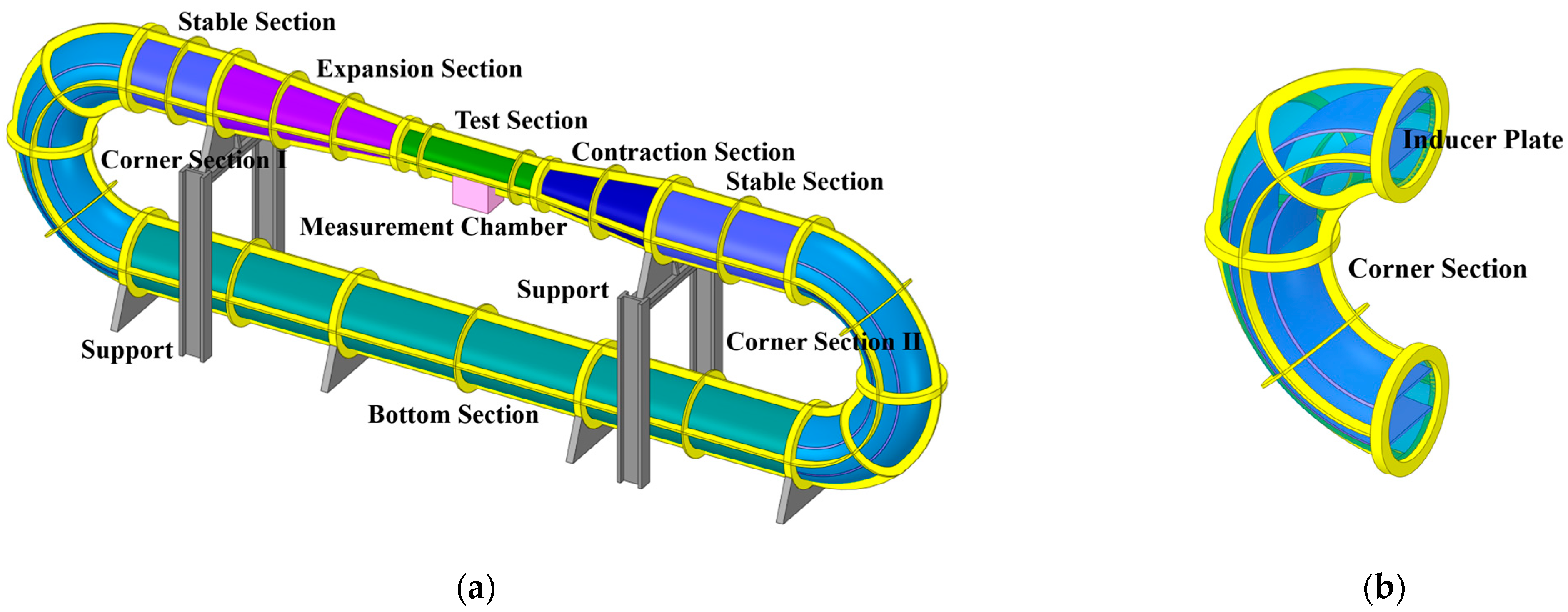
A 3D model of the water tunnel was developed based on the design specifications outlined in the literature reference [30]. The water tunnel comprises several components, including the test section, measurement chamber, contraction section, expansion section, stable sections, corner sections, bottom section, and rack, as shown in Figure 1a. The test section has a diameter of 180 mm and a length of 800 mm. The main pipeline of the water tunnel has a diameter of 350 mm. The contraction section and expansion section are conical pipes, with lengths of 700 mm and 1000 mm, respectively. Two 10 mm-thick inducer plates are installed inside the corner sections, with bending radii of 450 mm and 600 mm, as shown in Figure 1b.
The materials used for the construction of the water tunnel components vary depending on their specific functions. In this study, the test section and the measurement chamber are constructed using polymethyl methacrylate (PMMA), with a wall thickness of 25 mm. To enhance sound absorption within the measurement chamber, it is lined with sound-absorbing material, which has an absorption coefficient of 0.4 below 1 kHz. A 25 mm thick PMMA panel is installed between the test section and the measurement chamber. The remaining sections of the water tunnel are constructed using steel, with a wall thickness of 10 mm. To provide additional reinforcement, stiffeners with thickness of 10 mm are incorporated into the steel components. The different sections of the water tunnel are connected using flanges, which have a flange thickness of 20 mm. The material parameters for the various components of the water tunnel are summarized in Table 1.
3.2. Grid Division
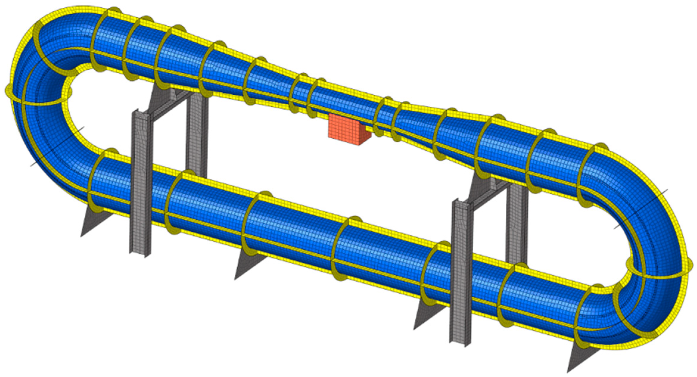
As the wall thickness of the main structure is relatively thin at 10 mm, it can be treated as a thin plate. Therefore, in order to ensure accuracy and improve computational efficiency, the structures of the water tunnel are modeled using shell elements to construct a finite element mesh model. The bending wave velocity of thin plate can be written as
where cp is the bending wave velocity, ω is the angular frequency, E is the Young’s modulus, h is the plate thickness, ρ0 is the density, and μ is the Poisson’s ratio. The minimum structural bending wave wavelength in the water tunnel, considering a minimum thickness of the steel plate of 10 mm and a maximum calculation frequency of 1 kHz, is determined to be 313.6 mm. To ensure accurate results, the finite element calculation should satisfy the criterion of having at least six elements within one bending wave wavelength. Based on this requirement, the maximum allowable size for structural elements is determined to be 52 mm, according to the requirement for the mesh, as shown in Figure 2.
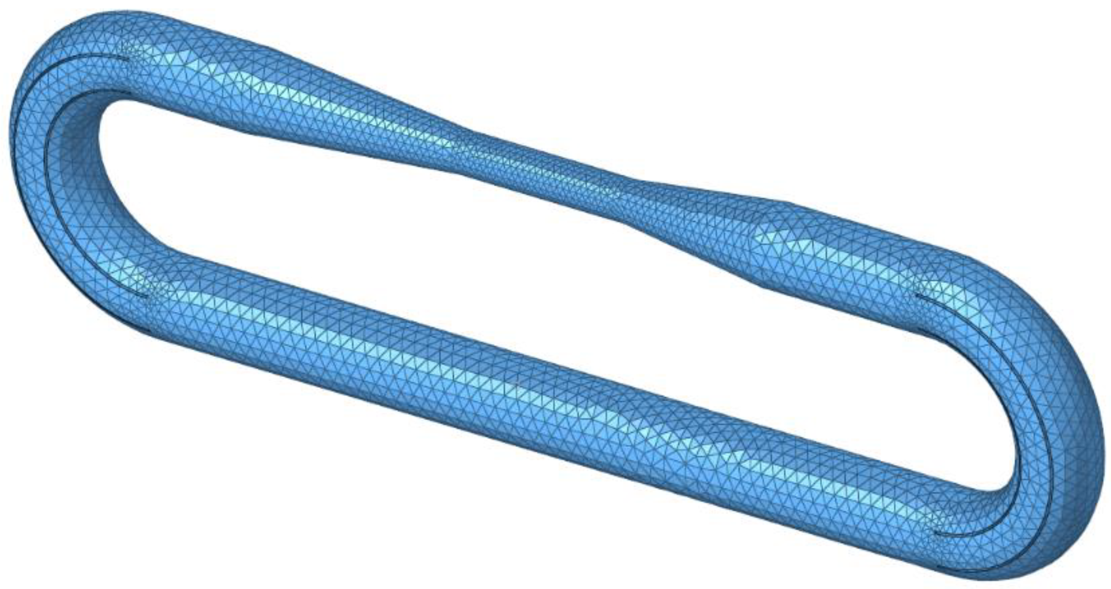
All the cavities inside the water tunnel are fluid domains and need to be divided into acoustic mesh. The acoustic wavelength in water can be written as
where λ is acoustic wavelength, is the sound velocity in water, and f is frequency. Thus, the minimum acoustic wavelength is 1500 mm at a maximum calculation frequency of 1 kHz. The acoustic mesh for finite element calculations also needs to satisfy the requirement of at least six elements within one acoustic wavelength, so the maximum acoustic mesh size is 250 mm, according to the requirement for meshing in the fluid domain, as shown in Figure 3.
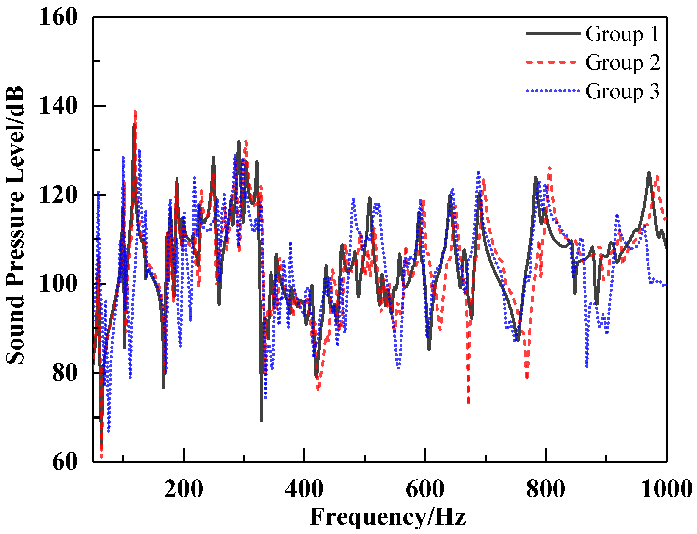
Prior to conducting the numerical simulation, an independent mesh verification process was performed to ensure the reliability and accuracy of the results. For this purpose, three sets of structural and acoustic meshes with different sizes were utilized. The element sizes and quantities for each mesh set are presented in Table 2.
The sound pressure level at the field point at the center of the test section is defined to check the mesh independence, as shown in Figure 4. It can be seen that the calculated results of the Group 1 and Group 2 agree with each other and the peaks basically match, and there is a difference between the calculated results of Group 2 and Group 3 after 800 Hz. Therefore, it can be concluded that the 40 mm structural mesh and the 150 mm acoustic mesh already satisfy the mesh independence requirements.
3.3. Flow Field
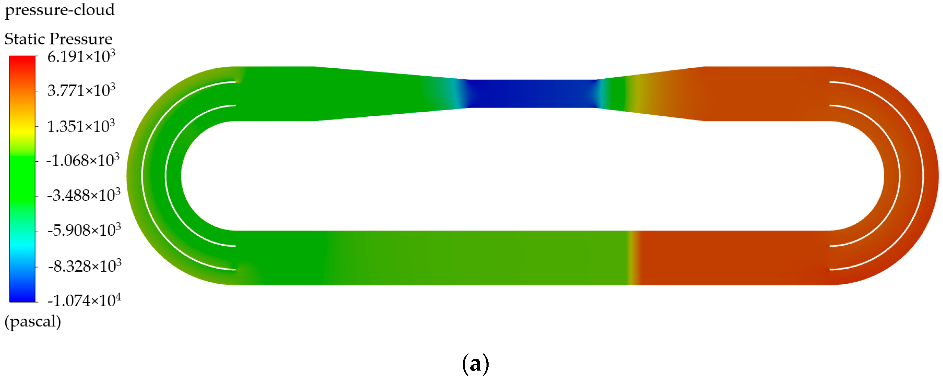
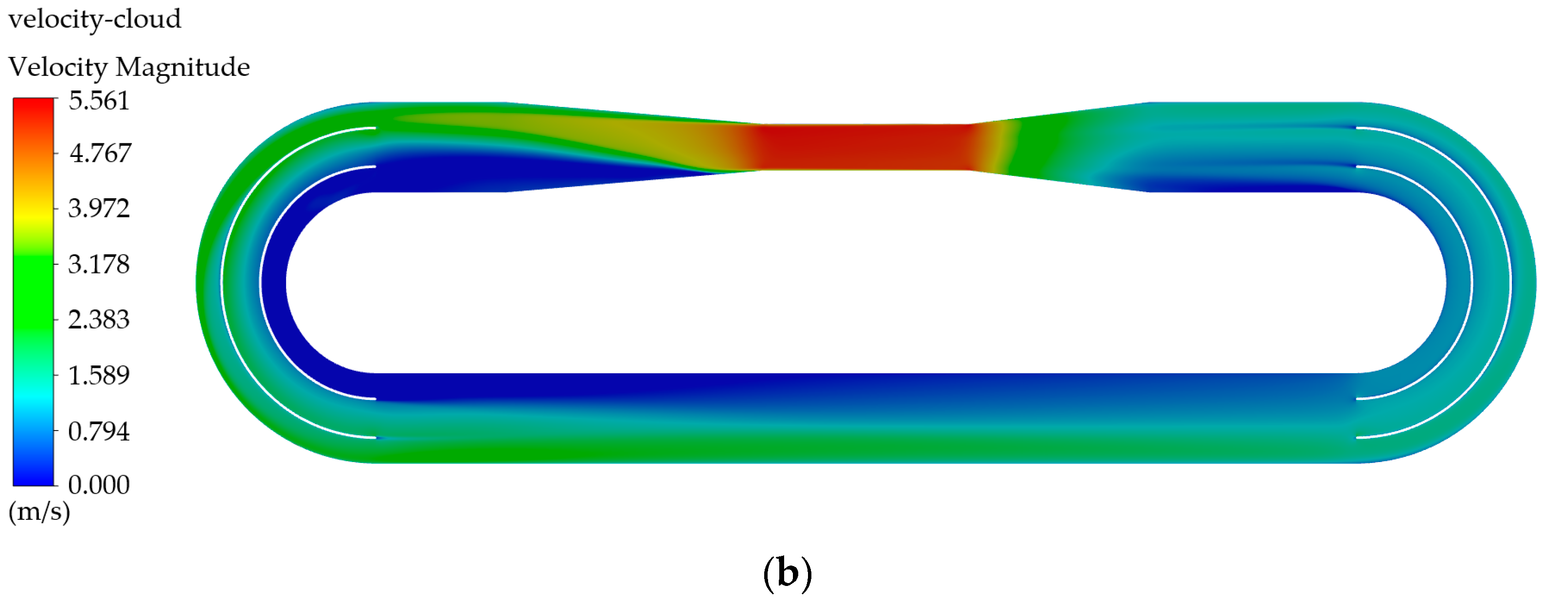
In this study, a delayed detached eddy simulation (DES) turbulence model based on the k-ω shear stress transport (k-ω SST) approach is employed to analyze the transient flow field inside a water tunnel. The computational time step is set at 0.0005 s. The water flow exhibits a counterclockwise circulation pattern within the tunnel. For modeling simplicity, the propeller impeller is replaced with a surface pressure drop representation. The test section operates at a flow velocity of 5.56 m/s. In consideration of the substantial size of the fluid domain, computational efficiency is a crucial concern. So, boundary layer grids within the fluid domain are established with a Yplus value of 30, while the first layer’s thickness at the boundary layer is maintained at 0.0126 mm. The total number of grids in the computational domain amounts to 19.95 million. The distribution of pressure and velocity in the longitudinal section of the flow field is illustrated in Figure 5.
3.4. Boundary Condition
Flow noise is calculated using acoustic finite element with a frequency interval of 1 Hz. The wall of the water tunnel structure is assumed to be rigid. The wall pressure pulses are interpolated to the acoustic mesh envelope and Fourier transformed and set as a surface dipole source as a boundary condition for the flow noise calculation.
In the fluid–solid interaction analysis, the surface of internal fluid is coupled to the inner wall of structure to form a fluid–solid coupling surface, while the wall pressure pulsations are interpolated onto the fluid–solid coupling surface for flow-excited noise calculation. Fixed constraints are applied to the ends of the support and bracing at the bottom of the water tunnel. The direct method of steady-state dynamics is used to calculate the vibration displacement of the water tunnel under the excitation of the wall pressure pulse, and then the vibration displacement is used to solve for the sound pressure response in the test section and the measurement chamber. The finite element calculation process is shown in Figure 6.
4. Results and Discussion
4.1. Characteristics of Flow Noise
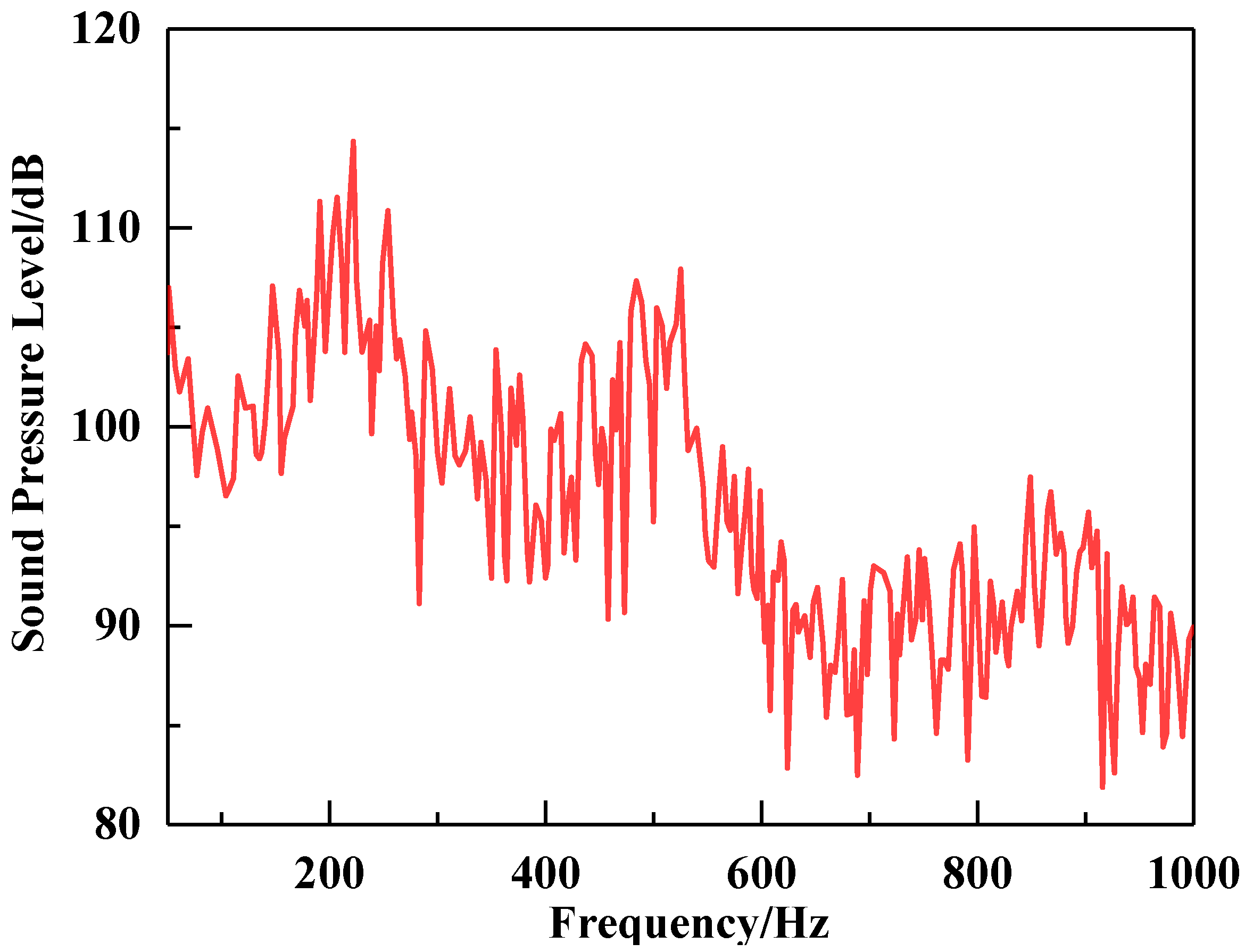
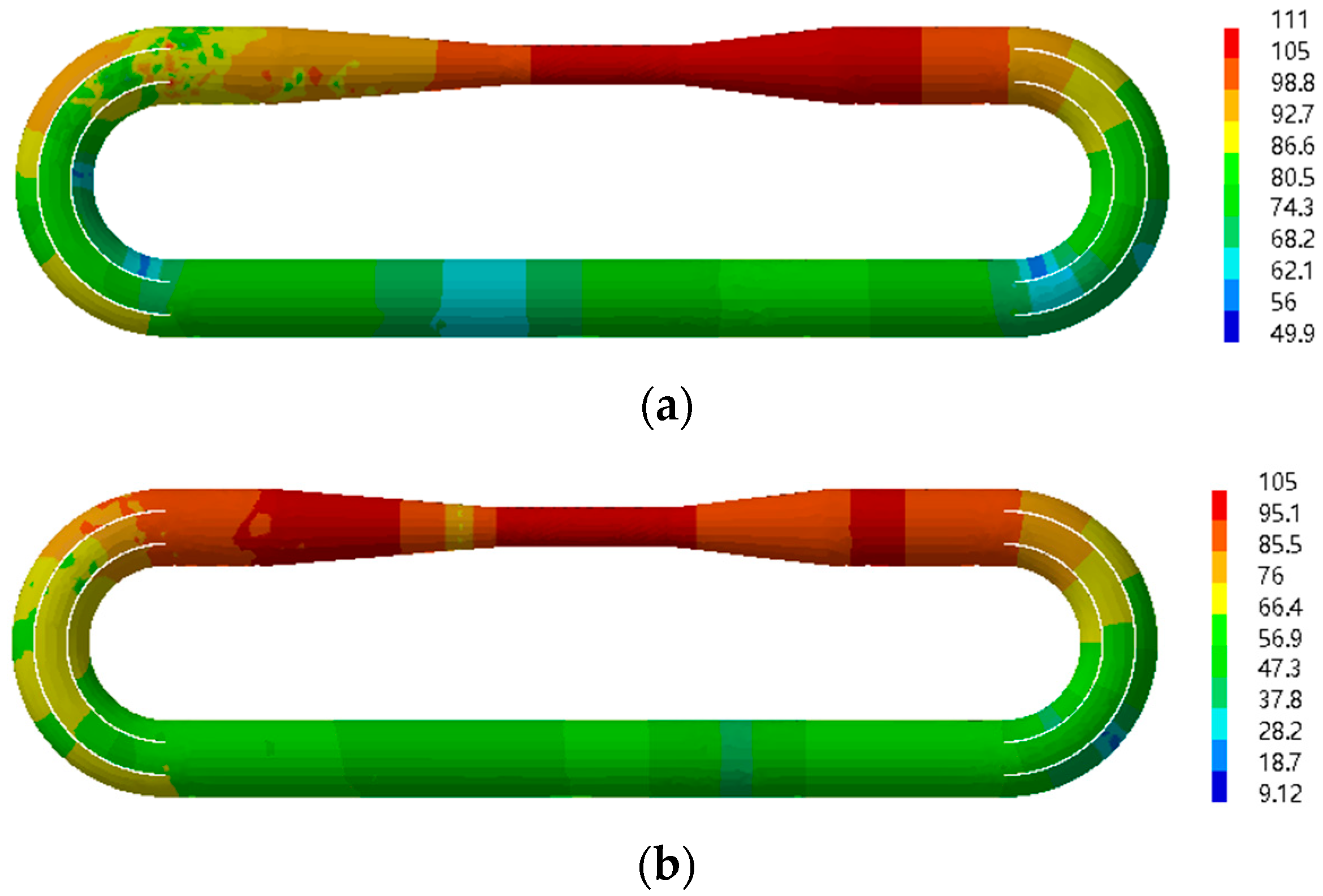
The flow noise in the fluid domain of the water tunnel due to wall pressure pulse was calculated using acoustic finite elements. The flow noise response curves for the center of the test section are shown in Figure 7. The data show that the overall trend of the flow noise decreases as the frequency increases within the range of 50 to 1000 Hz, with larger peaks at 254 Hz and 525 Hz. The sound pressure response cloud near 254 Hz and 525 Hz is shown in Figure 8. The distribution of internal sound pressure follows an axial pattern along the length of the water tunnel, resembling the shape of bamboo knots, and both have the largest sound pressure amplitudes at the test section.
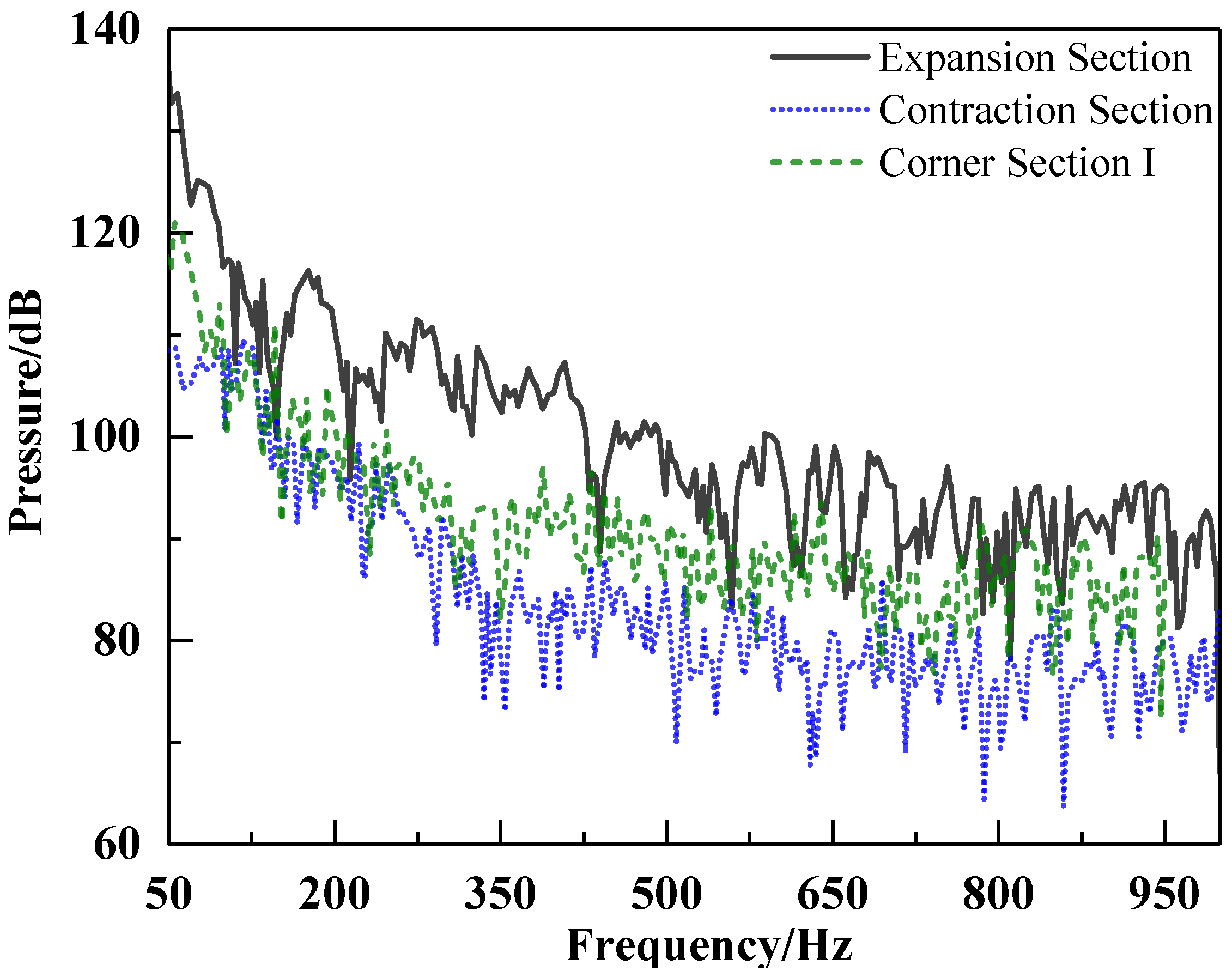
Due to the high degree of turbulence in the flow field in the contraction section, expansion section and corner section I, the wall pressure pulse curve at these sections is shown in Figure 9. The wall pressure pulse curve at the sections ranging from 50 to 1000 Hz gradually decreases with increasing frequency, which is consistent with the overall trend of the flow noise. However, the wall pressure pulse does not show significant peaks around 250 Hz and 500 Hz.
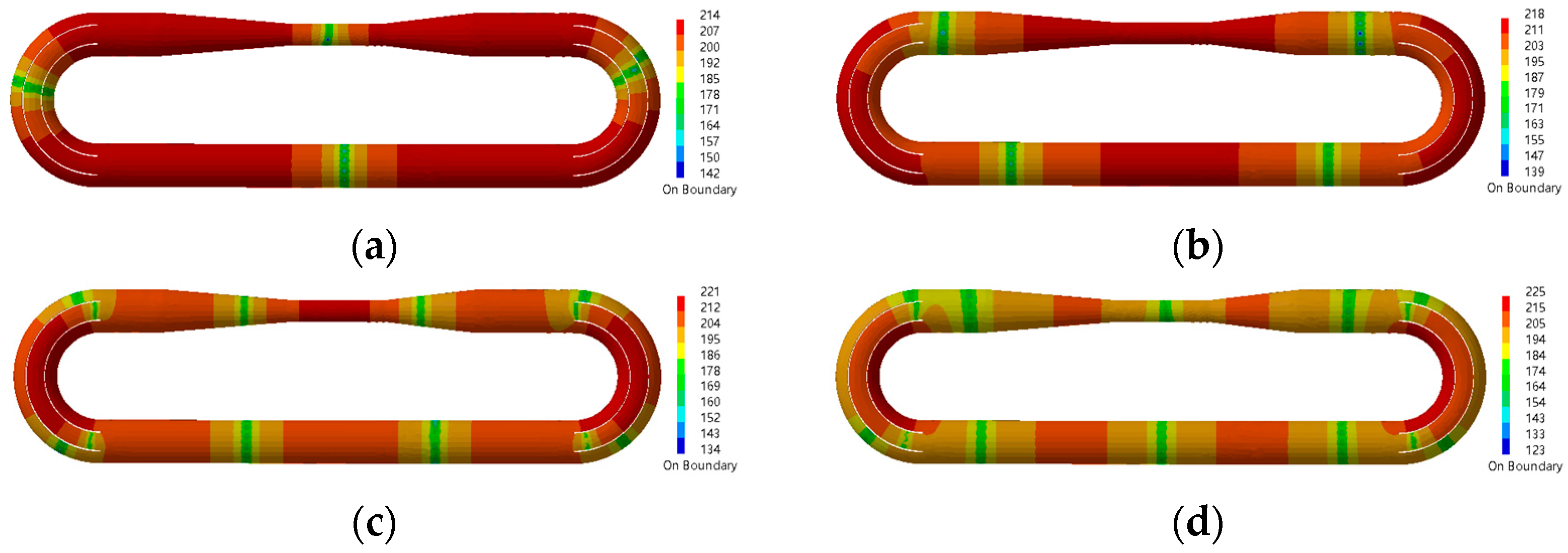
The acoustic modes in the fluid domain of the water tunnel were analyzed below 1000 Hz. Specifically, the acoustic modes around 250 Hz and 500 Hz were investigated and are presented in Table 3. Additionally, the corresponding acoustic mode distributions are depicted in Figure 10. It is evident that at these frequencies, the acoustic modes in the water tunnel exhibit a distinctive bamboo-like distribution. This distribution pattern indicates that the acoustic waves propagate as plane waves throughout the water tunnel. Comparing Figure 8 with Figure 10, it becomes apparent that the wall pressure pulse excites multiple acoustic modes within the water tunnel, leading to the formation of peaks in the flow noise response.
4.2. Characteristics of Flow-Excited Noise
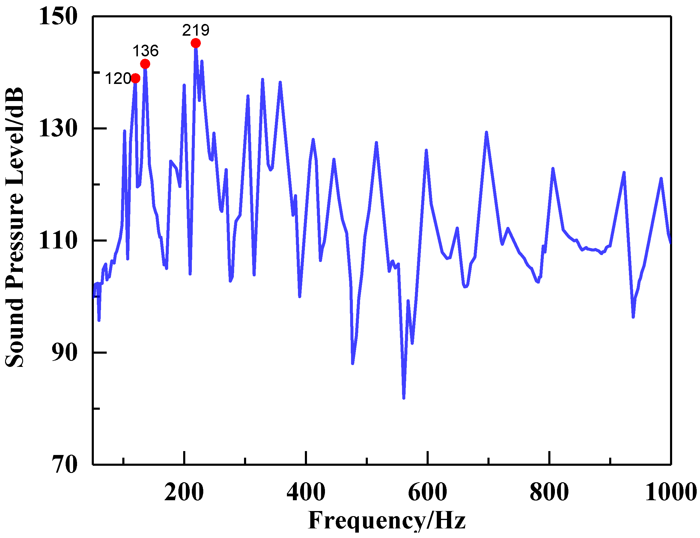
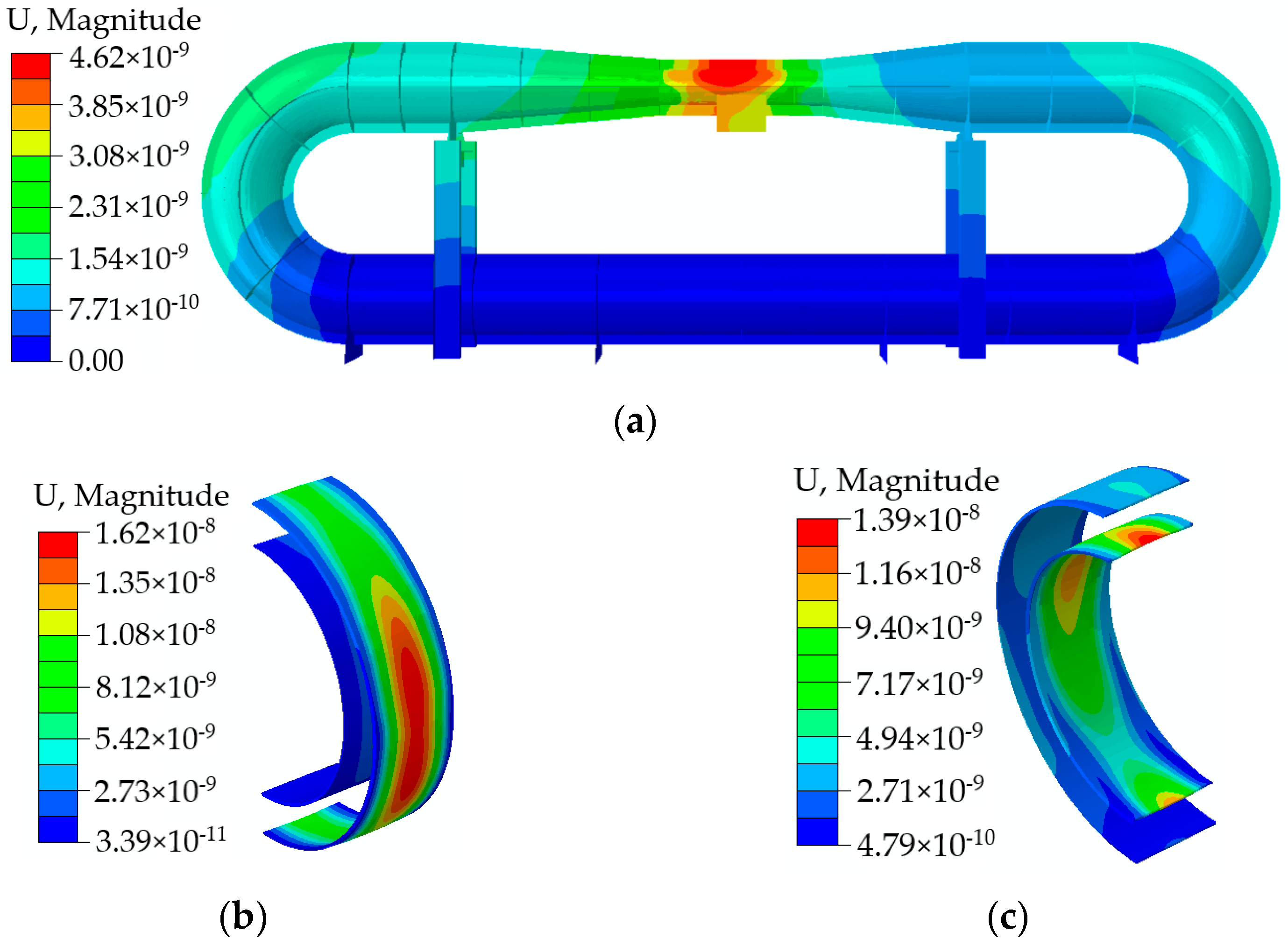
The unidirectional fluid–solid coupling calculation was used to obtain the noise radiated by the structure vibration due to the excitation of wall pressure pulses. The flow-excited response curve in the test section is obtained as shown in Figure 11. The curve exhibits a general decreasing trend across the frequency range of 50 to 1000 Hz. Notably, the curve displays several peaks, and the vibration displacement clouds corresponding to the peaks at 120 Hz, 136 Hz, and 219 Hz are illustrated in Figure 12. At 120 Hz, the maximum displacement occurs at the middle of the test section, while at 136 Hz, it is located in the middle of the inducer plate. Similarly, at 219 Hz, the maximum displacement is observed at the edge of the inducer plate. Upon examining the wall pressure pulse curves in Figure 9, it is evident that no peak wall pressure pulse coincides with the frequencies of 120 Hz, 136 Hz, and 219 Hz. Consequently, the peak sound pressure levels observed at these frequencies are not attributed to the excitation caused by wall pressure pulses.
The wet mode of the water tunnel was analyzed within the frequency range of 100 to 250 Hz, and the corresponding results are presented in Table 4. Furthermore, the mode shapes associated with frequencies of 119.81 Hz, 136.07 Hz, and 219.27 Hz are illustrated in Figure 13. By examining Figure 12 in conjunction with Figure 13, it can be observed that the responses at these three frequencies align with the frequencies and vibration patterns of the wet mode. It can be seen that the structural resonance is excited at 120 Hz and the maximum displacement is at the test section. At 136 Hz, the first order mode of the inducer plate is excited, forming a monopole radiation mode. Lastly, the edge mode of the inducer plate is excited at 219 Hz.
The further analysis of the subsequent peaks revealed that the prominent causes of the larger peaks were twofold. Firstly, the excitation of overall structural modes led to intensified structural vibrations, amplifying the amplitude of the peaks. Secondly, the local modes of the inducer plate are excited, leading to the generation of efficient radiation patterns. In light of these findings, it becomes evident that measures need to be implemented to mitigate and suppress these peaks.
4.3. Analysis of Background Noise Components
Flow noise caused by wall pressure pulse and flow-excited noise caused by flow-solid coupling effect are the main components of the water tunnel background noise. Analyzing the relative magnitudes of these two types of noise can provide insights into reducing the background noise across different frequency bands.
Figure 14 shows the comparison of flow noise, flow-excited noise, and total background noise in the water tunnel from 50 to 1000 Hz at a working condition of 5.56 m/s. It can be seen that the curves for the flow noise and the flow-excited noise follow a similar trend, both decreasing with increasing frequency. At this flow rate, the level of flow-excited noise is higher than that of flow noise in the 50–1000 Hz range, mainly due to the presence of numerous line spectra generated by structural resonance. As the line spectra of flow-excited noise are the main cause of high background noise, measures should be taken in the structural design of water tunnel to reduce these peaks in order to achieve lower background noise levels.
4.4. Analysis of Vibration and Noise Control
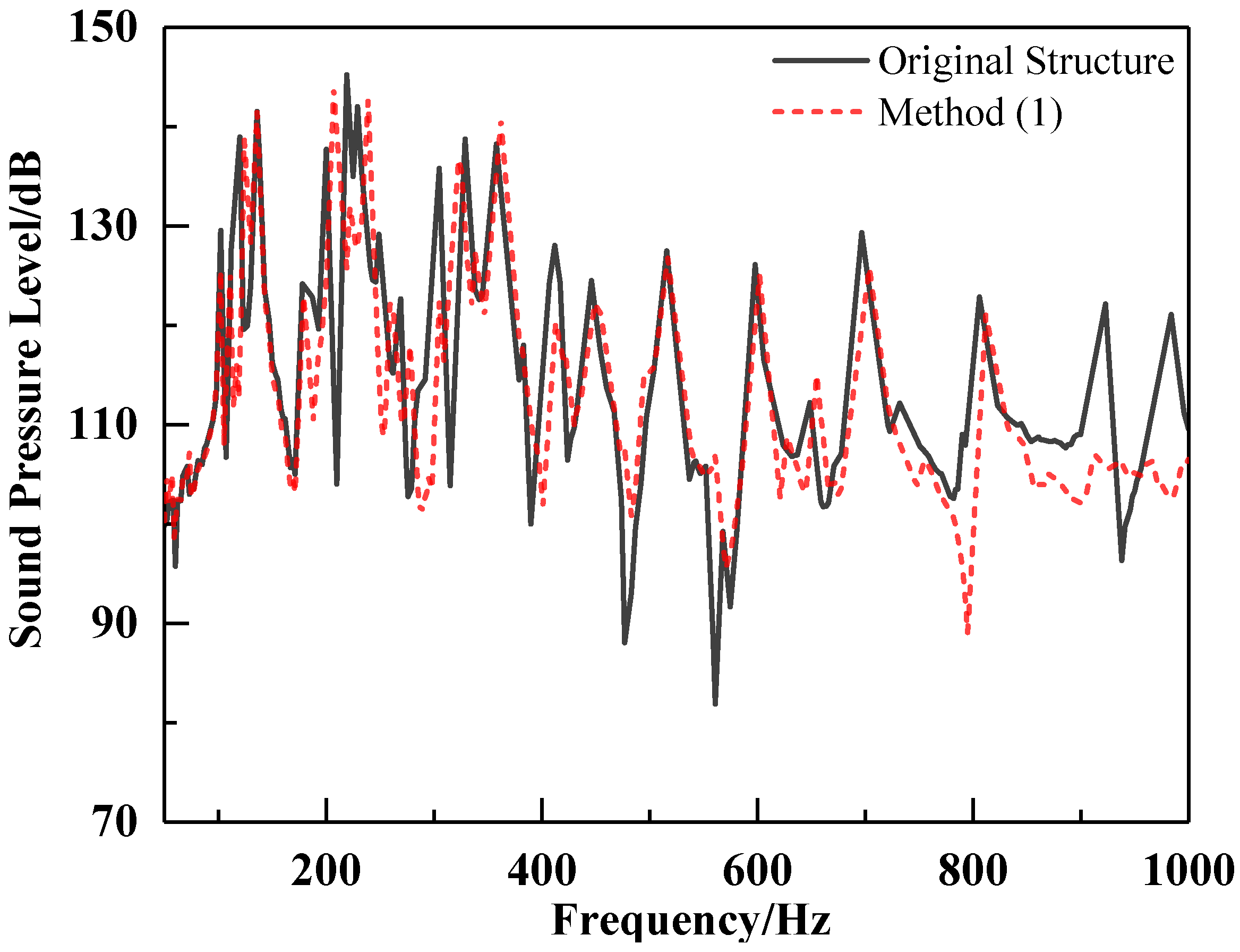
In water tunnel experiments, high background noise can interfere significantly with the experimental results, so measures need to be taken to reduce the background noise level within the test section. Based on the above analysis, the flow-excited noise peaks generated by structural resonance are the main components of the background noise and measures should be taken to suppress them. Three methods are proposed to investigate strategies for reducing structural vibration noise:
(1) Increase the number of longitudinal stiffeners on the outer wall of the contraction section, test section, and expansion section, as shown in Figure 15a.
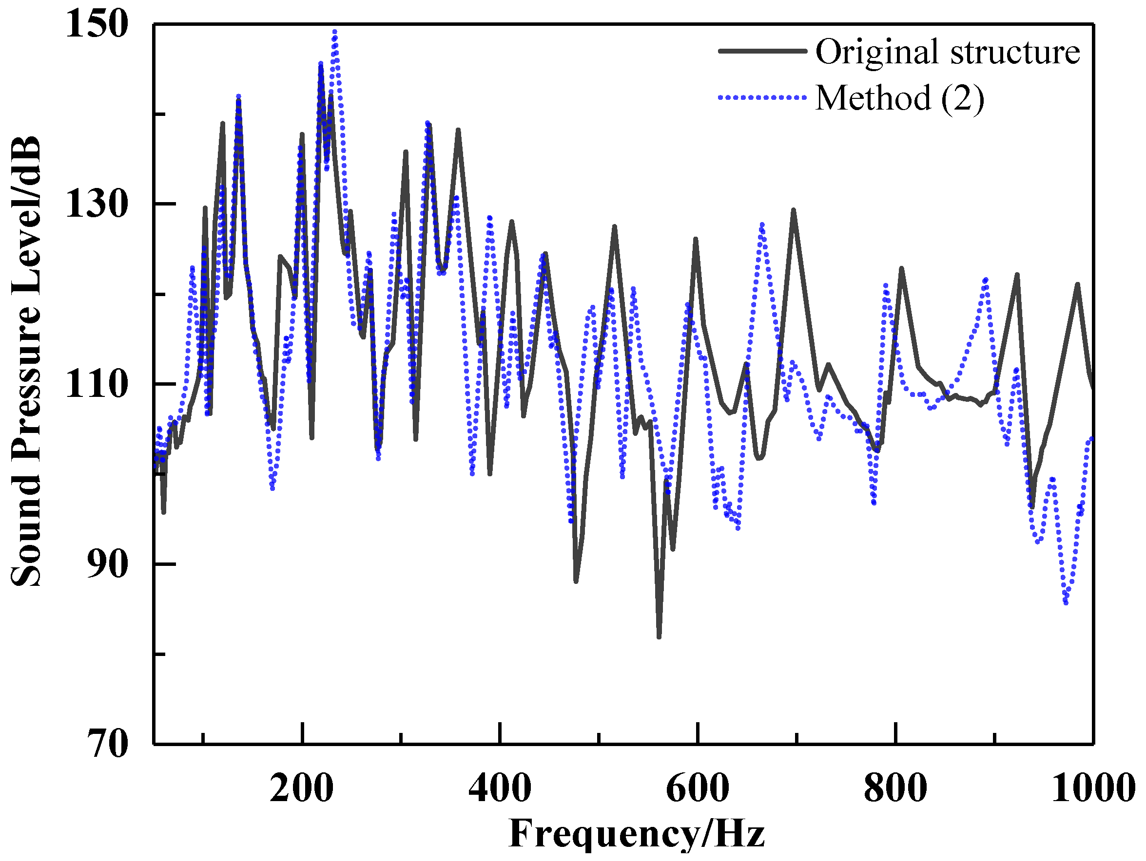
(2) Lay rubber damping material on the outer wall of the structure in the contraction section, test section, and expansion section, as shown in Figure 15b.
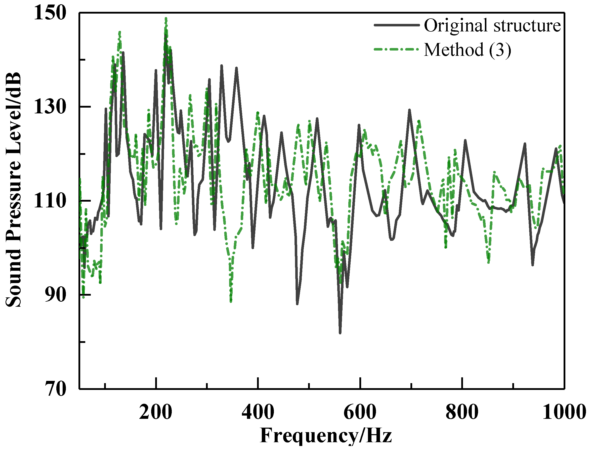
(3) Add two longitudinal bulkheads connected to the wall of the corner section on the inducer plate of the corner section, as shown in Figure 15c.
The flow-excited noise response in the test section was calculated and compared under the same wall pressure pulse, and the results are illustrated in Figure 16, Figure 17 and Figure 18. It can be observed that the flow-excited noise peaks at low frequencies do not exhibit a significant decrease using method (1). However, the level of flow-excited noise at high frequencies experiences a reduction, and the peak frequency shifts towards higher frequencies due to the increased stiffness of the structure by increasing the number of stiffeners. With method (2), the flow-excited noise curve is reduced by laying rubber damping material, and the peak frequency is shifted to lower frequencies because the damped natural frequency of the structure is lower than the undamped natural frequency. In method (3), the addition of longitudinal bulkheads to the inducer plate reduces some of the peak that would be generated via inducer plate vibration, because the stiffness of the inducer plate increases with the addition of longitudinal bulkheads, resulting in reduced vibration displacement.
In practical engineering applications, it is crucial to consider the three different structural improvement measures together to achieve comprehensive background noise suppression in water tunnels. Each measure targets specific aspects of noise reduction and contributes to an overall reduction in background noise levels. By combining these measures, their respective advantages can be leveraged to address different sources of noise and optimize the overall acoustic performance of the water tunnel.
4.5. Analysis of Vibration and Noise Control
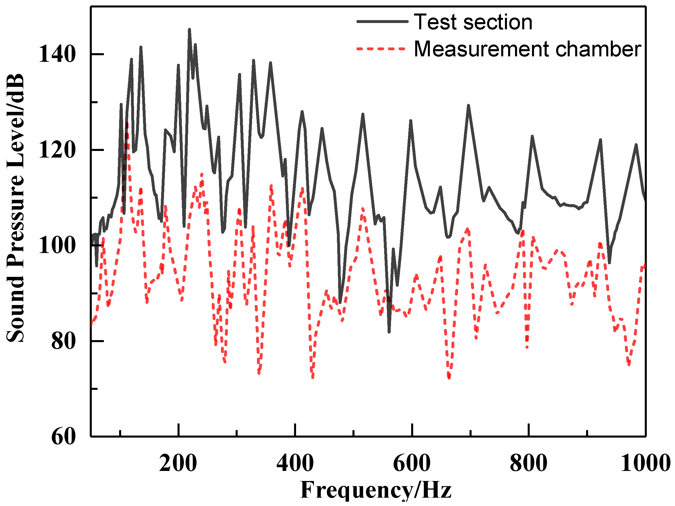
In this research, noise measurements were conducted using a hydrophone placed inside a measurement chamber that was suspended on the side of the test section. A PMMA plate was installed between the test section and the chamber to separate them. Based on the finite element model of the circulating water tunnel, the flow-excited noise response was calculated at two monitoring points in the test section and the chamber under wall pressure pulse, as shown in Figure 19. The results reveal the flow-excited noise response of the monitoring point in the test section is much higher than that of the monitoring point in the chamber in the range of 50 to 1000 Hz.
The water tunnel pipe in this study has a circular cross-section, and the cut-off frequency fc of the acoustic waveguide in the cylindrical pipe can be expressed as
where is the sound speed in water and a is the radius of pipe [31]. With a maximum radius of 175 mm, the cut-off frequency in the acoustic waveguide can be determined to be 2511 Hz. It is known that as long as the frequency of the acoustic source is below 2511 Hz, only the plane wave that propagates along the axial direction will be generated in the pipe. As the maximum calculated frequency is 1000 Hz, the acoustic wave in the water tunnel propagates axially along the pipe in the form of plane wave at frequencies below 1000 Hz.
At the PMMA plate, where the chamber is connected to the test section, the plane sound wave is incident at a large oblique angle, and the sound pressure reflection coefficient rp and the sound pressure transmission coefficient tp can be expressed as follows when plane sound wave is incident obliquely from medium I to medium II:
where m = ρ2/ρ1, ρ1 is the density of medium I and ρ2 is the density of medium II. When n = c1/c2, c1 is the sound velocity in medium I and c2 is the sound velocity in medium II. θi is the angle of incidence [31]. As c1 < c2, the sound pressure reflection coefficient rp ≈ 1 when the angle of incidence θi is large, resulting in only a small proportion of the sound waves with a small angle of incidence being able to pass through the PMMA plate. As a result, the sound pressure in the chamber is much lower than that in the test section below 1000 Hz.
As a result, when the frequency is far below the cut-off frequency of the acoustic waveguide, it is possible to measure the noise level within the test section by hanging the chamber on the side of the test section with a large error.
5. Conclusions
The numerical calculation model of the internal acoustic field and fluid–solid coupling of the water tunnel is established in this research. The numerical simulations of the flow noise and flow-excited noise in the water tunnel under wall pressure pulse are carried out using finite element software, and the characteristics of flow noise and flow-excited noise in the water tunnel are analyzed in detail, which provide some guidance for the practical engineering construction and optimization of water tunnels.
The overall trend of flow noise in the water tunnel aligns with the trend observed in the wall pressure pulse. Both exhibit a decreasing trend as the frequency increases. It is important to note that the flow noise spectrum displays peaks that are associated with the multi-order acoustic modes present in the fluid domain. In contrast, the flow-excited noise spectrum exhibits numerous peaks that are primarily caused by the excitation of overall and local modes of the structure through the wall pressure pulse. In water tunnels characterized by high flow velocities, the levels of flow-excited noise at low and medium frequencies are significantly higher than flow noise.
To achieve effective noise reduction, measures need to be implemented to mitigate or suppress these peaks in the flow-excited noise. The effectiveness of reducing vibration and noise in the structure by incorporating stiffeners and damping materials is found to be limited when it comes to attenuating low-frequency peaks. However, as the frequency increases, the noise reduction effect gradually improves. The inducer plates within the water tunnel are identified as significant sources of flow-excited noise peaks. By increasing the stiffness of the inducer plates by adding longitudinal bulkheads, it is possible to mitigate some of the resonance peaks associated with their vibration.
Below the cut-off frequency, the predominant mode of acoustic wave propagation takes the form of plane waves. This characteristic behavior impacts the accuracy of measuring low-frequency noise using a sound measurement chamber suspended on the side of the test section. The reliance on the chamber in this manner introduces a higher degree of error when assessing low-frequency noise levels in a water tunnel.
Author Contributions
Conceptualization, M.C. and T.W.; methodology, Z.H.; software, Z.H. and H.C.; validation, Z.H.; formal analysis, Z.H. and W.D.; investigation, Z.H. and H.C.; resources, H.C.; data curation, Z.H.; writing—original draft preparation, Z.H.; writing—review and editing, M.C., T.W., H.C. and W.D.; visualization, Z.H.; supervision, H.C. and W.D.; project administration, M.C. and T.W.; funding acquisition, M.C. and T.W. All authors have read and agreed to the published version of the manuscript.
Funding
This research was funded by National Key Laboratory of Electromagnetic Energy (grant number 614221722020302), the National Natural Science Foundation (grant number 52071152), the National Natural Science Foundation (grant number 52001131), and Young Elite Scientists Sponsorship Program by Cast (grant number 2022QNRC001).
Data Availability Statement
Not applicable.
Conflicts of Interest
The authors declare no conflict of interest.
References
- Tani, G.; Viviani, M.; Ferrando, M.; Armelloni, E. Aspects of the measurement of the acoustic transfer function in a cavitation tunnel. Appl. Ocean Res. 2019, 87, 264–278. [Google Scholar] [CrossRef]
- Amailland, S.; Thomas, J.H.; Pézerat, C.; Boucheron, R. Boundary layer noise subtraction in hydrodynamic tunnel using robust principal component analysis. J. Acoust. Soc. Am. 2018, 143, 2152–2163. [Google Scholar] [CrossRef] [PubMed]
- Song, H.; He, Y.; Yan, X.; Dajing, S. A numerical simulation of flow-induced noise from cavity based on LES and Lighthill acoustic theory. In Proceedings of the IEEE/OES China Ocean Acoustics Symposium, Harbin, China, 9–11 January 2016. [Google Scholar]
- Jia, D.; Zou, Y.C.; Pang, F.Z.; Miao, X.H.; Li, H.C. Experimental study on the characteristics of flow-induced structure noise of underwater vehicle. Ocean Eng. 2022, 262, 112126. [Google Scholar] [CrossRef]
- Ren, Y.; Qin, Y.X.; Pang, F.Z.; Wang, H.F.; Su, Y.M.; Li, H.C. Investigation on the flow-induced structure noise of a submerged cone-cylinder-hemisphere combined shell. Ocean Eng. 2023, 270, 113657. [Google Scholar] [CrossRef]
- Croaker, P.; Skvortsov, A.; Kessissoglou, N. A simple approach to estimate flow-induced noise from steady state CFD data. In Proceedings of the ACOUSTICS, Gold Coast, Australia, 2–4 November 2011. [Google Scholar]
- Zhu, W.J.; Shen, W.Z.; Sørensen, J.N. High-order numerical simulations of flow-induced noise. Int. J. Numer. Methods Fluids 2011, 66, 17–37. [Google Scholar] [CrossRef]
- Jonson, M.L.; Shepherd, M.R.; Myer, E.C.; Hambric, S.A.; DeRoche, R.J. Numerical characterization of the background noise generated by the ARL/PENN state garfield Thomas water tunnel impeller. In Proceedings of the ASME International Mechanical Engineering Congress and Exposition, Lake Buena Vista, FL, USA, 13–19 November 2009. [Google Scholar]
- Zhang, N.; Xie, H.; Wang, X.; Wu, B.S. Computation of vortical flow and flow induced noise by large eddy simulation with FW-H acoustic analogy and Powell vortex sound theory. J. Hydrodyn. 2016, 28, 255–266. [Google Scholar] [CrossRef]
- Zhang, N.; Shen, H.C.; Yao, H.Z. Numerical simulation of cavity flow induced noise by LES and FW-H acoustic analogy. J. Hydrodyn. 2010, 82, 242–247. [Google Scholar] [CrossRef]
- Wei, L.; Zhu, G.R.; Qian, J.Y.; Fei, Y.; Jin, Z.J. Numerical Simulation of Flow-Induced Noise in High Pressure Reducing Valve. PLoS ONE 2015, 10, e0129050. [Google Scholar] [CrossRef] [PubMed]
- Yao, H.L.; Zhang, H.X.; Liu, H.T.; Jiang, W.C. Numerical study of flow-excited noise of a submarine with full appendages considering fluid structure interaction using the boundary element method. Eng. Anal. Bound. Elem. 2017, 77, 1–9. [Google Scholar] [CrossRef]
- Abshagen, J.; Schafer, I.; Will, C.; Pfister, G. Coherent flow noise beneath a flat plate in a water tunnel experiment. J. Sound Vib. 2015, 340, 211–220. [Google Scholar] [CrossRef]
- Kudo, T.; Nishimura, M.; Sawada, S.; Mori, T.; Sato, R. Noise prediction of the cavitation tunnel. In Proceedings of the Fluids Engineering Division Summer Meeting, Honolulu, HI, USA, 6–10 July 2003. [Google Scholar]
- Kim, J.; Sung, H.J. Wall pressure fluctuations and flow-induced noise in a turbulent boundary layer over a bump. J. Fluid Mech. 2006, 558, 79–102. [Google Scholar] [CrossRef]
- Mori, M.; Masumoto, T.; Ishihara, K. Study on acoustic, vibration and flow induced noise characteristics of T-shaped pipe with a square cross-section. Appl. Acoust. 2017, 120, 137–147. [Google Scholar] [CrossRef]
- Shi, S.K.; Tang, W.H.; Huang, X.C.; Dong, X.Q.; Hua, H.X. Experimental and numerical investigations on the flow-induced vibration and acoustic radiation of a pump-jet propulsor model in a water tunnel. Ocean Eng. 2022, 258, 111736. [Google Scholar] [CrossRef]
- Maryami, R.; Arcondoulis, E.J.; Liu, Q.; Liu, Y. Experimental near-field analysis for flow induced noise of a structured porous-coated cylinder. J. Sound Vib. 2023, 551, 117611. [Google Scholar] [CrossRef]
- Lecoffre, Y.; Chantrel, P.; Teiller, J. Le Grand Tunnel Hydrodynamicpie (GTH): France’s New Large Cavitation Tunnel for Hydrodynamics Research. Int. Symp. Cavitation Res. Facil. Tech. 1987, 54, 1–10. [Google Scholar]
- Wetzel, J.M.; Arndt, R.E.A. Hydrodynamic Design Considerations for Hydroacoustic Facilities: Part I—Flow Quality. J. Fluids Eng. 1994, 116, 324–331. [Google Scholar] [CrossRef]
- Wetzel, J.M.; Arndt, R.E.A. Hydrodynamic Design Considerations for Hydroacoustic Facilities: Part II—Pump Design Factors. J. Fluids Eng. 1994, 116, 332–337. [Google Scholar] [CrossRef]
- Brandner, P.A.; Lecoffre, Y.; Walker, G.J. Design considerations in the development of a modern cavitation tunnel. In Proceedings of the 16th Australasian Fluid Mechanics Conference, Gold Coast, Australia, 2–7 December 2007. [Google Scholar]
- Boucheron, R.; Amailland, S.; Thomas, J.H.; Pezerat, C.; Frechou, D.; Briancon-Marjollet, L. Experimental modal decomposition of acoustic field in cavitation tunnel with square duct section. In Proceedings of the Meetings on Acoustics 173EAA, Boston, MA, USA, 25–29 June 2017. [Google Scholar]
- Doolan, C.; Brandner, P.; Butler, D.; Pearce, B.; Moreau, D.; Brooks, L. Hydroacoustic characterisation of the AMC cavitation tunnel. In Proceedings of the Acoustics 2013 Victor Harbor: Science, Technology and Amenity, Victor Harbor, Australia, 17–20 November 2013. [Google Scholar]
- Lauchle, G.C.; Bistafa, S. Acoustic source strength measurements of cavitation noise in a water tunnel. J. Acoust. Soc. Am. 1989, 85, S115. [Google Scholar] [CrossRef]
- Boucheron, R. Modal decomposition method in rectangular ducts in a test-section of a cavitation tunnel with a simultaneous estimate of the effective wall impedance. Ocean Eng. 2020, 209, 107491. [Google Scholar] [CrossRef]
- Park, C.; Kim, G.D.; Park, Y.H.; Lee, K.; Seong, W. Noise localization method for model tests in a large cavitation tunnel using a hydrophone array. Remote Sens. 2016, 8, 195. [Google Scholar] [CrossRef]
- Li, Z.G.; Zhan, F.L. Virtual. Lab Acoustics Advanced Application Example of Acoustic Simulation Calculation; National Defense Industry Press: Beijing, China, 2010; pp. 7–14. [Google Scholar]
- Huo, R.D. Research on Numerical Method of Flow-Induced Noise of Ship Structure; Harbin Engineering University: Harbin, China, May 2020. [Google Scholar]
- Liu, M.S. Design of Cavitation Water Channel for Simulating the Hydrodynamic Environment of High Speed Underwater Moving Bodies; Nanjing University of Science and Technology: Nanjing, China, January 2014. [Google Scholar]
- Du, G.H.; Zhu, Z.M.; Gong, X.F. Fundamentals of Acoustics; Nanjing University Press: Nanning, China, 2012; pp. 183–191. [Google Scholar]
Figure 1.
A 3D geometric model: (a) water tunnel; (b) corner section.

Figure 2.
Structural Mesh.

Figure 3.
Acoustic Mesh.

Figure 4.
Sound pressure level at the field point at the center of the test section.

Figure 5.
(a) Pressure distribution and (b) velocity distribution in the longitudinal section of the flow field.
Figure 5.
(a) Pressure distribution and (b) velocity distribution in the longitudinal section of the flow field.


Figure 6.
Finite element calculation flowchart.

Figure 7.
Flow noise response curves for the center of the test section.

Figure 8.
Flow noise response cloud at (a) 254 Hz and (b) 525 Hz.

Figure 9.
Wall pressure pulse curve of contraction section, expansion section and corner section I.

Figure 10.
Acoustic mode clouds of the fluid domain at (a) 258.15 Hz, (b) 295.06 Hz, (c) 495.87 Hz, and (d) 519.76 Hz.
Figure 10.
Acoustic mode clouds of the fluid domain at (a) 258.15 Hz, (b) 295.06 Hz, (c) 495.87 Hz, and (d) 519.76 Hz.

Figure 11.
Flow-excited noise response curves for the center of the test section.

Figure 12.
Vibration displacement clouds of (a) 120 Hz, (b) 136 Hz, and (c) 219 Hz.

Figure 13.
Mode shapes of (a) 119.81 Hz, (b) 136.07 Hz, and (c) 219.27 Hz.

Figure 14.
Flow noise, flow-excited noise, and total background noise in the water tunnel.

Figure 15.
Diagram of (a) method (1), (b) method (2), and (c) method (3).


Figure 16.
Flow-excited noise response curves of original structure and method (1).

Figure 17.
Flow-excited noise response curves of original structure and method (2).

Figure 18.
Flow-excited noise response curves of original structure and method (3).

Figure 19.
Flow-excited noise response curves of test section and sound measurement chamber.


Table 1.
Material parameters.
| Material Name | Density | Young’s Modulus | Poisson’s Ratio | Sound Speed |
|---|---|---|---|---|
| PMMA | 1180 kg/m3 | 3 GPa | 0.35 | 2020 m/s |
| Steel | 7850 kg/m3 | 210 GPa | 0.3 | 5800 m/s |
Table 2.
Structural and acoustic mesh parameters.
| Group | Structural Mesh | Acoustic Mesh | Mesh Quantity |
|---|---|---|---|
| Group 1 | 35 mm | 100 mm | 114,126 |
| Group 2 | 40 mm | 150 mm | 67,724 |
| Group 3 | 45 mm | 200 mm | 39,340 |
Table 3.
Acoustic modes of the fluid domain.
| Order | 3 | 4 | 9 | 10 |
|---|---|---|---|---|
| Acoustic mode | 258.15 Hz | 295.06 Hz | 495.87 Hz | 519.76 Hz |
Table 4.
Wet mode of the water tunnel.
| Order | 10 | 11 | 12 |
|---|---|---|---|
| Frequency | 119.81 Hz | 136.07 Hz | 219.27 Hz |
Disclaimer/Publisher’s Note: The statements, opinions and data contained in all publications are solely those of the individual author(s) and contributor(s) and not of MDPI and/or the editor(s). MDPI and/or the editor(s) disclaim responsibility for any injury to people or property resulting from any ideas, methods, instructions or products referred to in the content. |
© 2023 by the authors. Licensee MDPI, Basel, Switzerland. This article is an open access article distributed under the terms and conditions of the Creative Commons Attribution (CC BY) license (https://creativecommons.org/licenses/by/4.0/).
Share and Cite
MDPI and ACS Style
Huang, Z.; Chen, M.; Wang, T.; Cui, H.; Dong, W. Numerical Investigation of Background Noise in a Circulating Water Tunnel. Machines 2023, 11, 839. https://doi.org/10.3390/machines11080839
AMA Style
Huang Z, Chen M, Wang T, Cui H, Dong W. Numerical Investigation of Background Noise in a Circulating Water Tunnel. Machines. 2023; 11(8):839. https://doi.org/10.3390/machines11080839
Chicago/Turabian StyleHuang, Zhangkai, Meixia Chen, Ting Wang, Huachang Cui, and Wenkai Dong. 2023. "Numerical Investigation of Background Noise in a Circulating Water Tunnel" Machines 11, no. 8: 839. https://doi.org/10.3390/machines11080839
Note that from the first issue of 2016, this journal uses article numbers instead of page numbers. See further details here.