
A Global Path Planning Method for Unmanned Ground Vehicles in Off-Road Environments Based on Mobility Prediction


1
Hefei Institutes of Physical Science, Chinese Academy of Sciences, Hefei 230031, China
2
Science Island Branch, University of Science and Technology of China, Hefei 230026, China
*
Author to whom correspondence should be addressed.
Machines 2022, 10(5), 375; https://doi.org/10.3390/machines10050375
Submission received: 15 April 2022
/
Revised: 7 May 2022
/
Accepted: 12 May 2022
/
Published: 16 May 2022
(This article belongs to the Topic Advances in Mobile Robotics Navigation)
Abstract
:In a complex off-road environment, due to the low bearing capacity of the soil and the uneven features of the terrain, generating a safe and effective global route for unmanned ground vehicles (UGVs) is critical for the success of their motion and mission. Most traditional global path planning methods simply take the shortest path length as the optimization objective, which makes it difficult to plan a feasible and safe route in complex off-road environments. To address this problem, this research proposes a global path planning method, which considers the influence of terrain factors and soil mechanics on UGV mobility. First, we established a high-resolution 3D terrain model with remote sensing elevation terrain data, land use and soil type distribution data, based on a geostatistical method. Second, we analyzed the vehicle mobility by the terramechanical method (i.e., vehicle cone index and Bakker’s theory), and then calculated the mobility cost based on a fuzzy inference method. Finally, based on the calculated mobility cost, the probabilistic roadmap method was used to establish the connected matrix and the multi-dimensional traffic cost evaluation matrix among the sampling nodes, and then an improved A* algorithm was proposed to generate the global route.
1. Introduction
Due to their unnecessary requirement of human interference and their ability to replace human operations in risky environments, unmanned ground vehicles (UGVs) have several applications, such as disaster rescue, nuclear inspection, planet exploration and military operations, etc. In order to enable a UGV to traverse complex off-road environments quickly and safely and achieve its missions, an effective global path planning method is required, of which the key objective is to generate a safe and feasible route from the initial position to the specified targets based on given off-road environmental map information [1,2].
In recent decades, path planning methods developed rapidly, resulting in numerous new such methods [3]. Path planning methods can be mainly divided into two categories, i.e., graph search-based and sampling-based [3]. Typical graph search-based methods include Dijkstra, A*, D*, field D* and several other variants [4,5,6,7]. The graph search-based path planning methods can find the optimal path accurately, but such algorithms should traverse the surrounding of the current node and select the minimum cost node, which leads to large computational efforts. To reduce the calculation time the algorithm takes to search each interval, an efficient A* algorithm was proposed [8]. Guruji et al. [9] proposed an online path planning method for a mobile robot in a grid-map environment, using a modified real time A* algorithm. In obstacle-avoidance path planning, Duan et al. introduced a safety–cost matrix in the A* algorithm and the heuristic function was modified to ensure the optimal safety path in different environments [10].
Compared with graph search-based methods, sampling-based path planning methods have fast search efficiency, and classical sample-based approaches include rapidly exploring random trees (RRT) [11], probabilistic road maps (PRM) [12] and several other variants [13]. However, the random nature of sampling may lead to the tendency of falling into the local minimum in complex environments [14]. To address this problem, a potentially guided intelligent bi-directional RRT* algorithm was proposed [15], and the proposed algorithm greatly improved the convergence rate and had more efficient memory utilization. Also, Park et al. proposed a hierarchical roadmap (HRM) approach that enabled the indoor mobile robot to cover navigable areas using fewer nodes than a probabilistic roadmap [16].
However, most existing developed planning methods focus on structured environments, such as indoor and urban scenarios. Due to the low bearing capacity of the soil and the uneven features of the terrain, existing methods are very difficult to apply to complex unstructured off-road environments. To adapt to the off-road environments, researchers have proposed several improved planning methods based on traditional methods. For example, to evaluate the comprehensive influence of terrain slope and surface attributes, an improved A* algorithm with a window moving method was proposed; this method can plan a gentle global route for the mobile robot, while the robot can effectively avoid moving obstacles [17]. Similarly, a method was proposed to systematically deal with the effects of kinematic vehicle models, off-road terrains and obstacles to UGV path planning by constructing artificial potential fields [18]. Also, there is an increased risk of vehicle obstruction due to soil deformation. Gonzalez et al. [19] proposed a path planning method based on the classification of terrain into GO/NOGO areas by soil strength value (CI); it is worth mentioning that the method was integrated into the next-generation NATO reference mobility model (NG-NRMM). With the purpose of generating a high confidence global route in the off-road, Jiang et al. [20] employed a global path planning method based on the RRT* algorithm with the cost function of the uncertainty in terrain elevation. In terms of global path smoothing, the geometric curve method transforms the path planning problem into a two-point boundary value problem, such as the B-spline curve [21] and fifth degree polynomial curve [22].
In spite of progress, most existing global path planning methods ignore the effects of soil deformation on vehicle mobility. Although Gonzalez et al. proposed classifying off-road terrain into GO and NOGO based on the soil strength value (CI), it is still difficult to plan an optimal global route for UGV within the GO areas because of the lack of a well-designed cost function to quantify the effects of vehicle–terrain interaction. To address this problem, the contributions of this study are as follows: (1) In order to obtain 3D models of unknown off-road environments effectively, this paper proposes a Kriging terrain interpolation method based on open-source remote sensing DEM data with multi-source data fusion, which is general and easy to implement. (2) To address the problem that the current global path planning methods for unmanned vehicles do not take into account the impact of soil deformation on mobility, this paper proposes an analysis method based on terramechanical theory to calculate the impact of soil deformation on the speed of a UGV. Then, a method to quantify the cost of mobility based on fuzzy inference fusion of multiple influencing factors is proposed. (3) In terms of a global path generation algorithm, an improved A* algorithm based on mobility cost is proposed to generate a topological map by sampling terrain points, and to introduce mobility costs, in both extended cost and heuristic cost, to generate an efficient, feasible and safe global route. Finally, the effectiveness of the proposed method is validated by simulation and comparison experiments.
2. Methods
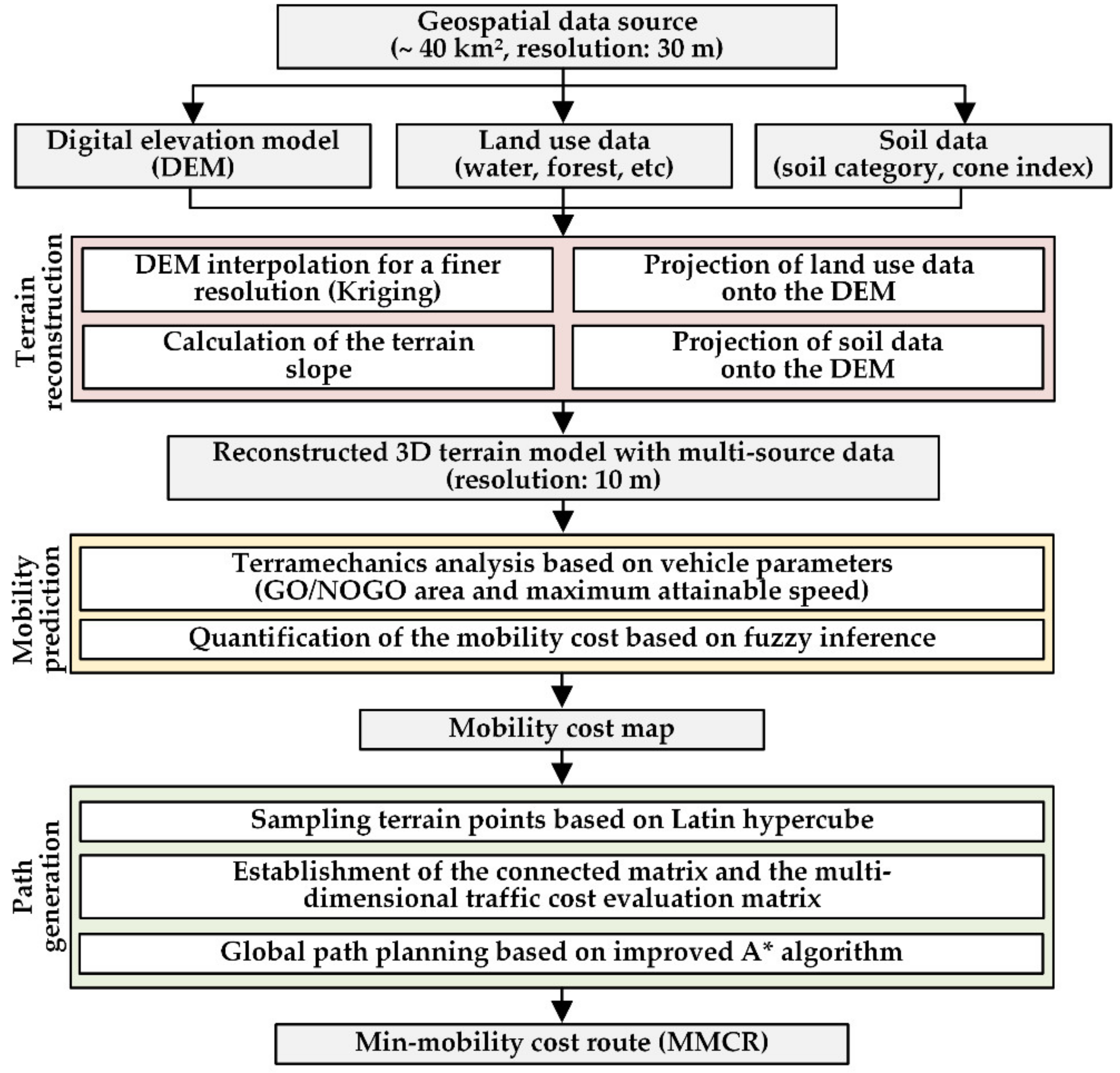
The proposed global planning method include three phases, i.e., terrain reconstruction, mobility prediction and path generation. In the terrain reconstruction phase, the original sparse digital elevation model (DEM) is firstly converted into a high-resolution 3D point cloud using a geostatistics interpolation method, and then the land use and soil type distribution data are integrated to generate a multisource terrain model. In the mobility prediction phase, the vehicle cone index and Bakker’s theory-based terramechanical model is proposed to calculate the maximum attainable speed of the UGV on different soil areas, and a fuzzy inference method is utilized to generate the global mobility cost map. In the path generation phase, an improved A* algorithm with extended cost and heuristic cost based on the mobility cost map is proposed to generate an optimal global route. Figure 1 shows the method framework.
2.1. Terrain Reconstruction
Terrain geometry information typically comes from remote sensing sources (e.g., radar, imagery camera, etc.). Since the resolution of the original DEM is too sparse for accurate prediction of vehicle mobility, an interpolation process is required to obtain a refined terrain model with a higher resolution. In our study, open-source remote sensing topographic data with a resolution of 30 m was used as the raw data; the required resolution for mobility prediction is usually about 10 m [23]. To further characterize other features of the selected terrain, the obtained land use data and soil type distribution data were projected onto the resulting refined DEM data. The reconstruction result was saved in the form of a 3D point cloud for the following processes.
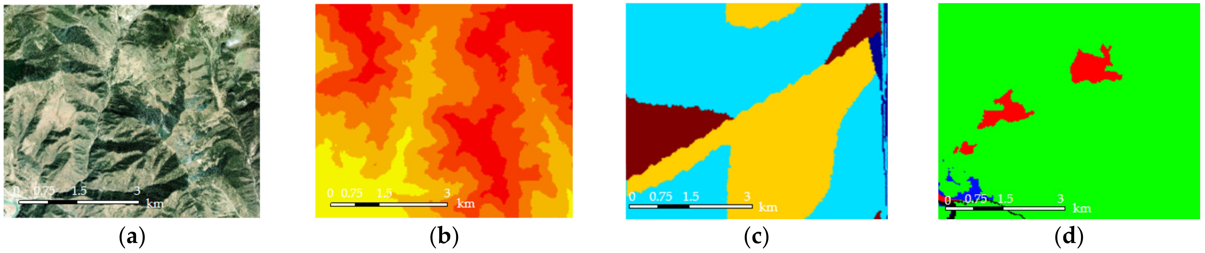
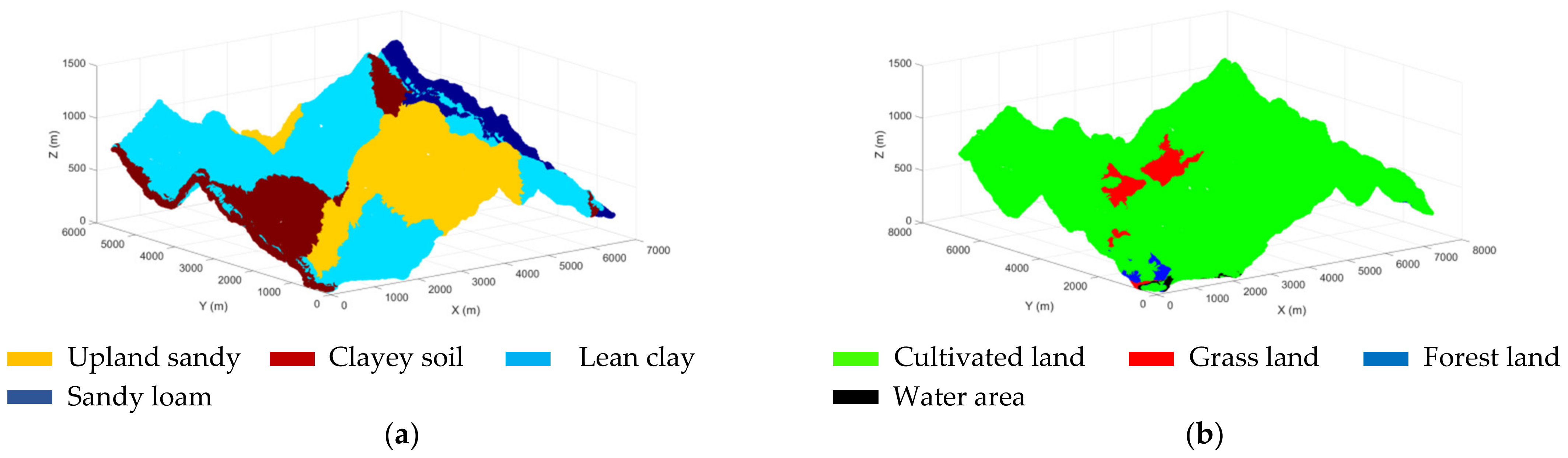
In this research, we selected a target area of about 40 km² within the range of 97.2°–97.3° E and 31.4°–31.5° N. After determining the target area, the satellite map and the DEM were downloaded on the geospatial data cloud website. In addition to elevation, the file contains a layer with different soil regions classified according to the National Earth System Science Data Center. Specifically, there are four soil types include sandy loam, clayey soil, lean clay and upland sandy. Also, land use data can be obtained using the method described above, and the data include water area, forest land, grass land and cultivated land. All the data are shown in Figure 2.
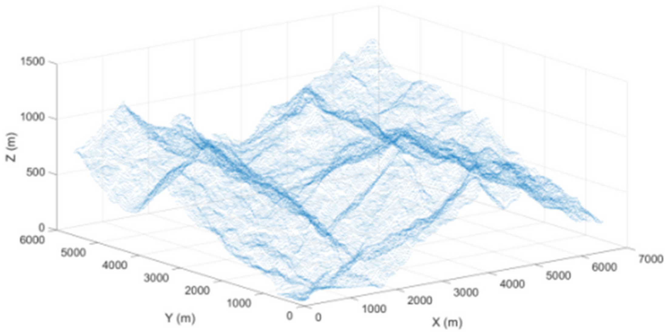
In the process of reconstructing the terrain, we needed to obtain the coordinates of the DEM data from the geographic coordinates (Longitude–Latitude). This preprocessing process generates the new DEM data in the Cartesian format. Each location was then formatted in terms of planar coordinates (X-Y) and elevation (Z), all of which are in metric units. The resulting 3D terrain model is displayed in Figure 3; the soil type distribution data and the land use data were also projected onto the corresponding terrain points (see Appendix A.1 the Projection of each Data Type.
The process of natural terrain modeling begins with a sparse set of measurements obtained from remote sensors on the terrain area of interest. An important step in simulating the performance of a UGV on such terrain is to generate a continuous surface; this process can be achieved by interpolating the elevations of unknown terrain points from the known terrain points. The most widely used terrain interpolation method in geostatistics is the Kriging [24], which is based on the principle of estimating the elevations of interpolated points from the variance of the known points. The variogram represents the statistical relationship between terrain points. This shows how the heterogeneity between and evolves with the lag distance ; its calculation formula is
where N is the number of terrain points, is the elevation at point and represents the separation distance, which is the vector separating the locations of two variables. For example, d is the separation distance between points. If points are sampled at 10 m, then d = 10 and the semi-variogram is calculated for the separation distance .
When the variogram model has been built, the Kriging method can be used for the terrain interpolation. There are three main forms of Kriging, depending on whether the mean of the data is known (simple Kriging) or unknown (ordinary Kriging and universal Kriging). In geostatistics, the most common method used is the ordinary Kriging [24], because the mean is not a priori and only spatial variation is meaningful. According to the ordinary Kriging formula, every terrain point with an unknown elevation is interpolated based on a weighted combination of the known terrain points, the expression being
where is the predicted elevation of the sample located at (interpolated terrain point) and are the weights for the combination of the known terrain points The parameter i represents the samples available in the dataset. Ordinary Kriging minimizes the mean squared error of prediction, and its expression is
After differentiating Equation (3) and setting the derivative to zero, it follows that
where is the Lagrange parameter used for ensuring . By using matrix expressions, the previous set of equations can be written as
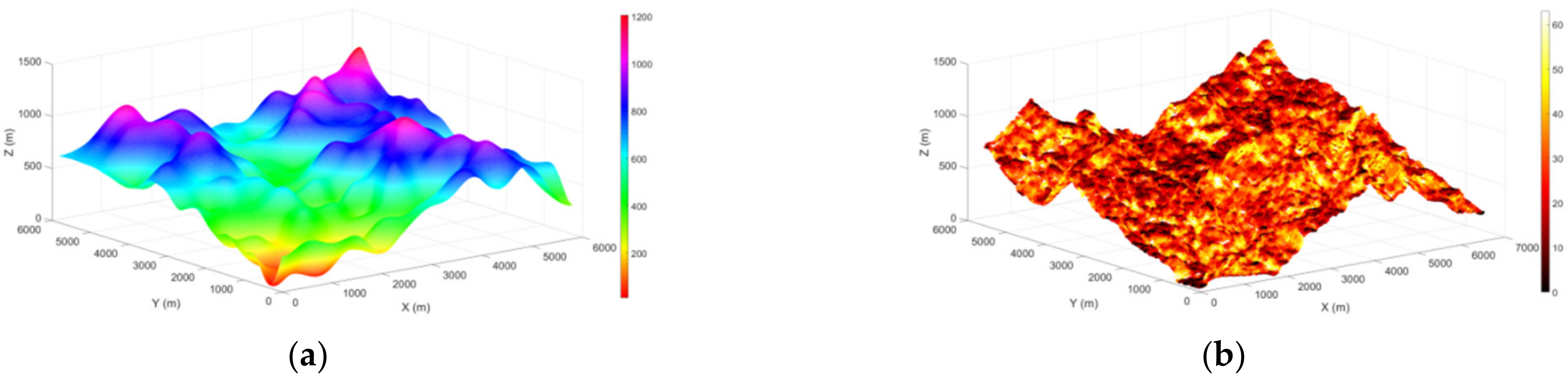
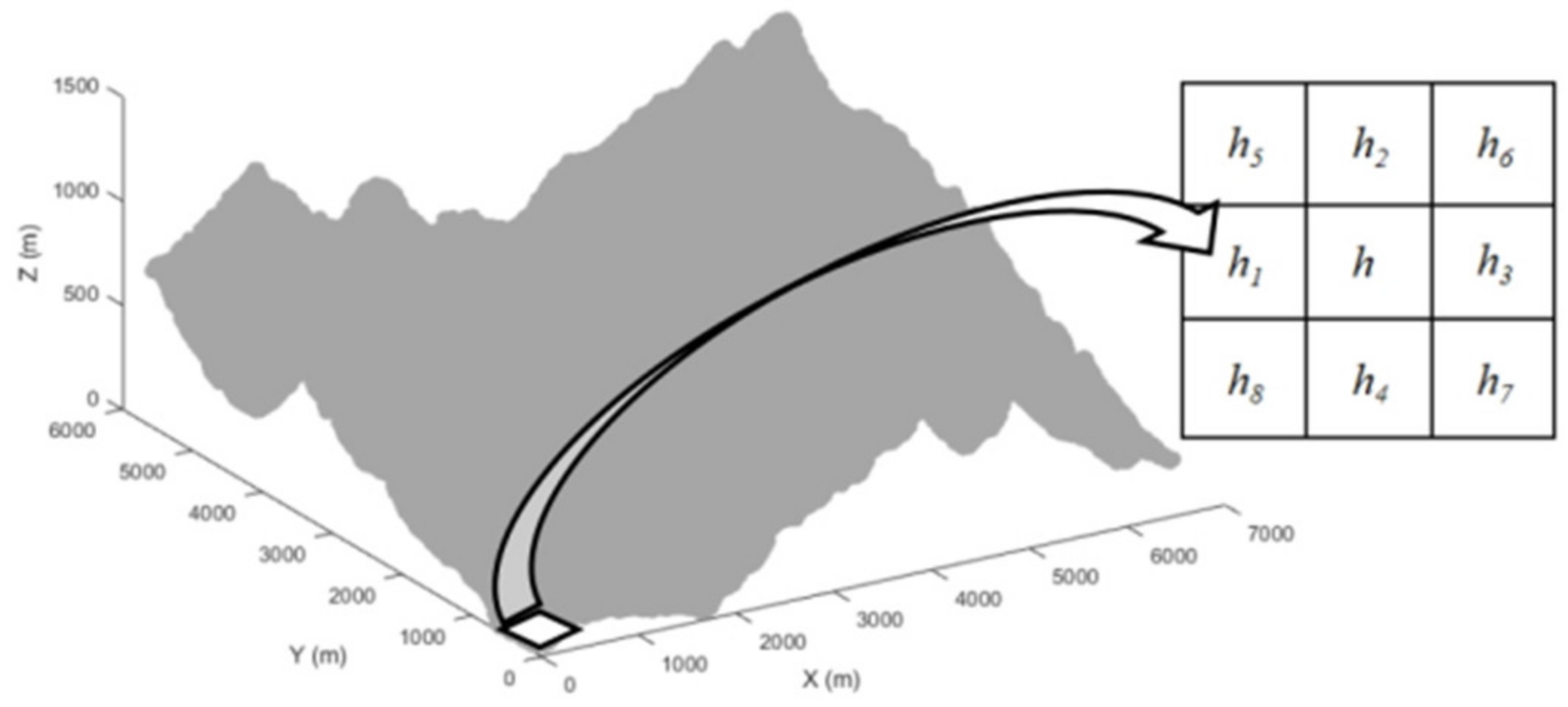
Once the weights are calculated, the predicted elevations at the unknown locations can be estimated using Formula (2). The reconstructed DEM is shown in Figure 4a. The slope of the terrain is also an important factor in limiting the mobility of the vehicle, as large slope angles can cause the vehicle to roll over. Therefore, after obtaining the refined 3D terrain model, the slope value of each terrain point is calculated. Specifically, a window template is used to traverse all points of the terrain; the slope map is shown in Figure 4b (see Appendix A.2 Slope Calculation Method).
2.2. Terramechanic Analysis
The off-road vehicle mobility prediction model is usually employed in the mobility-analysis phase to map environmental variables, such as soil properties, for example, into the vehicle mobility (vehicle maximum attainable speed). Various theoretical models were developed; for instance, the U.S. Army Engineer Research and Development Center (ERDC) defines vehicle mobility in two different ways. One is the single vehicle cone index (VCI1) and the other is the fifty-pass vehicle cone index (VCI50) [25]. VCI1 and VCI50 represent the minimum soil strength required for a vehicle to consistently make a specific number of passes. In the NATO Reference Mobility Model (NRMM) [26], VCI is used as a metric to evaluate the off-road mobility of military ground vehicles on different soils. The mobility performance is judged by the following:
- ·
- If CI VCI50, pass easily
- ·
- If VCI50 > CI VCI1, pass difficultly
- ·
- If CI < VCI1, not pass
Where CI (cone index) refers to the ratio of the force required to vertically press the cone penetrometer into the soil at a certain depth at a speed of 0.5 cm/s to the area of the cone. The value of VCI is related to the vehicle mobility index (MI), which is related to the ground pressure coefficient, axle load coefficient, tire coefficient, anti-skid coefficient, engine coefficient and transmission coefficient of the vehicle, reflecting the overall mobility of the vehicle. The expression of MI is
where is grounding pressure coefficient, is the engine coefficient, is the track tooth coefficient or wheel spur coefficient, is the tire coefficient, is the load factor, is the ground clearance and is the transmission coefficient.
According to the MI, the empirical formula can be used to calculate the VCI values of a single pass and fifty passes [25], which are VCI1 and VCI50, respectively.
For single-pass wheeled vehicles with MI ≤ 115:
For single-pass wheeled vehicles with MI > 115:
For wheeled vehicles with 50 passes:
To express the interaction between the vehicle and the ground, Bakker measured the mechanical properties of foundation soil experimentally [27], then Bakker’s derived terramechanic model (BDTM) was created. This model was applied to the NATO Reference Mobility Model (NRMM) to obtain the mobility prediction of military vehicles. In particular, when the structural parameters of the vehicle are known, the maximum attainable speed of the vehicle on a soft soil foundation mainly depends on soil characteristics. Considering these, BDTM is used to calculate the maximum attainable speed.
This paper takes wheeled unmanned vehicles as the object of analysis, when the pneumatic tire traverses off-road, it rolls in different states due to the different strengths of the soil. When the soil is soft and the sum of the tire inflation pressure generated by the tire stiffness is greater than the support force of the soil to the lowest point of the tire, the pneumatic tire rolls like a rigid tire; this phenomenon is referred to as the rigid mode of the tire, shown in Figure 5a. In contrast, on relatively solid soil, the tread-grounding parts of tires will be pressed into a plane, also known as the elastic mode, as shown in Figure 5b.
To calculate the maximum attainable speed of the vehicle, it is necessary to predict rolling resistance (). When the tire rolls on the soft soil, it forms a rut with a depth of , and the contact surface between the tire and the soil is divided into two areas, the curved surface and the plane. According to the pressure and sinkage relationship of BDTM, the calculated unit pressure in the curved surface area is
The unit pressure in the plane area is
where , and n are Bakker’s soil parameters, b is the tire width and is the sinkage.
Assuming that the diameter of the rigid wheel is , if the reaction force of the soil on the rigid wheel is only radial, the soil resistance () of the wheel can be obtained as
In the rigid mode, the soil is compressed only in the vertical direction, so the value of calculated from Equation (12) should be equal to the work done when a flat plate of width is pressed vertically into the soil to a depth of . The vertical load on the wheel is
This can be obtained from the geometric relationship of each variable:
Combine Equations (13) and (14):
Since the speed of a UGV traversing soft soil is very low, the air resistance factor is usually ignored. According to the principle of dynamic balance, the maximum speed that a UGV may achieve on soft soil is
where is the rated power of the engine and is the terrain slope.
In the elastic mode, the resistance effect caused by the elastic deformation of the tire must be considered. If a part of the tire is flattened and its projection length is L, the contact stress of this part is
According to Equation (11), the sinkage of the tire at this time is
Substitute Equation (19) into Equation (12) to obtain:
Similarly, after obtaining the resistance of the soil, the maximum speed that the vehicle may reach can be calculated according to Equation (17).
2.3. Mobility Cost Quantification
As described above, mobility prediction methods usually divide the terrain into GO and NOGO [19], where GO represents the area where the vehicle can traverse and NOGO is the opposite. The terrain points with slopes greater than the kinematic limits of the UGV are marked as NOGO, while soil areas with a CI less than VCI are marked as NOGO. Nevertheless, it is difficult for decision-makers to determine an optimal route for the UGV to travel from the GO areas. Consequently, it is necessary to quantify the mobility of the UGV in the GO areas. In the process of quantifying mobility, the influence of terramechanics and terrain parameters should also be considered.
However, the multi-factor fusion process cannot be simply weighted, so a fuzzy logic-based multi-factor fusion method is used. Fuzzy logic is a technique which uses the degree of truth instead of discrete values such as 0 or 1; it also uses “linguistic” variables such as “low”, “medium”, and “high”, as well as numerical variables for the calculations. The relationship between inputs and outputs is given by some simple statements rather than complex mathematical equations [28]. Let be a fuzzy subset. We can represent as
where is the degree of membership of in fuzzy subset . The membership degree has a value between 0 and 1. For a fuzzy subset , if , then , if , then , if possibly in , but not sure, then . The block diagram of the proposed fuzzy mobility cost quantification process is shown in Figure 6.
Combining the terramechanics and the fuzzy inference method, the terrain is then divided into NOGO, safe (high), low-risk (medium) and high-risk areas (low), and the mobility cost of each terrain point is converted into a distribution between [0, 1]: the closer the value is to 1, the worse the mobility. The rules need to be further analyzed in the context of specific vehicle and terrain characteristics, and this process is presented in Section 3.2 of this paper. For the determination of the membership function, in general, the steeper its shape, the higher the resolution of the system, the slower the change and the better the stability of the system [29]. Therefore, the membership functions corresponding to “low”, “medium” and “high” are Z-type, triangular type and S-type, respectively, as shown in Figure 7, and the corresponding expressions are listed in Equation (22).
For the fuzzy inference method, no consistent theory has been established to guide the construction of fuzzy relations, implying that the construction of fuzzy relations is diverse, the related fuzzy operations are different and the final inference results are not the same. A relatively simple and effective algorithm based on “Max–min” criterion is widely adopted in the practical use of fuzzy inference [30]. The “Max–min” criterion, also known as the pessimistic criterion, is one of the decision criteria for uncertainty-based decision making, and the basic attitude of this approach is conservative. It is implemented by finding the worst possible outcome of each option, i.e., the minimum value, and then selecting the option that provides the maximum payoff, i.e., the maximum value, among its worst outcomes. This guides one to maximize the minimum possible outcome. In order to avoid the risk of damage to the UGV during the off-road mission as much as possible, the “Max–min” criterion is, therefore, used in this case for defuzzification to obtain relatively conservative mobility prediction results.
2.4. Path Generation
In the global path planning method, it is necessary to build the topological relationships of the grids and plan the optimal route according to the topological relationships. In the traditional method, the topological relationships are usually established based on the distance between grids and the distribution of obstacles. Nevertheless, in large off-road terrains (>5 × 5 km) considering multiple influencing factors, traditional topological relationship-building methods cannot meet the requirement of generating a feasible, safe and effective global route. In this section, we propose a method to construct topological relations based on the above quantified results of mobility. Because of the large number of terrain points, the terrain points are sampled by the Latin hypercube sampling (LHS) method, and the sampled terrain points are used as the nodes for establishing topological relations. The topological relations of each node are then constructed based on the above quantified results of the mobility cost. The specific topological relationships are built based on the extended cost evaluation matrix and the heuristic cost evaluation matrix. With the topological relations, an improved A* algorithm is used for global path planning.
According to the results of the fuzzy process, the terrain is divided into NOGO area (), low-risk area (), high-risk area () and safe area (). All the areas are coupled into the total environmental area .
To build the topological relationship between each node, the sampling terrain points are first generated by Latin hypercube sampling, and the topological map is formed: P is the set of sampling nodes and E is the set of road sections between sampling points. The connectivity matrix is then used for connectivity evaluation, as shown in Figure 8a and the expression is
where is the connectivity matrix between the sampling nodes. If the straight line between two certain nodes and passes through , then its connectivity cost = 0, otherwise = 1.
The extended cost evaluation matrix includes the extended low-risk cost matrix , extended high-risk cost matrix , extended distance cost matrix and extended safe-cost matrix . For instance, the extended low-risk cost matrix consists of the low-risk cost between the nodes in set P. The evaluation method is to take n uniformly distributed sampling nodes on the straight line between two nodes and ; the low-risk is evaluated by the cost accumulation of each child node in the low-risk area and the evaluation results are indicated as the low-risk cost matrix of the path between multiple nodes, as shown in Figure 8b; its expression is
Similarly, the extended high-risk cost matrix and the extended safe-cost matrix can be obtained, as shown in formulas:
The distances between the nodes also need to be considered in node expansion, so the extension distance cost matrix is composed of Euclidean distance between the nodes in set P, as shown in Figure 8c, and its expression is
To improve the efficiency of path planning and to optimize the expansion direction of nodes, it is necessary to consider the heuristic cost evaluation between the new expansion node and the goal node , and search along the path direction with the least heuristic cost. Therefore, the heuristic cost evaluation matrix includes the heuristic barrier cost matrix , the heuristic distance cost matrix and the heuristic safe cost matrix . is composed of the heuristic barrier cost between the node and the goal node . It is evaluated using the cumulative sum of the cost of the NOGO areas and the cost of the risk area where each child node is located in the path between the sampling nodes and the goal node, as shown in Figure 8d, so the expression is , and .
The heuristic distance cost matrix consists of the Euclidean distance between the node and the goal node ; its expression is , and .
The heuristic safe cost matrix consists of the heuristic safe cost between the node and the goal node . It is evaluated by accumulating the cost of the safe area, where each child node is located in the path between the sampling nodes and the goal node, and its expression is and .
The global path planning method based on the extended cost evaluation function and the heuristic cost evaluation function designed in this paper is
where is the cost evaluation function from the start node to the current node and is the extended cost evaluation function from the start node to the current node ; is the heuristic cost evaluation function from the current node to the goal node .
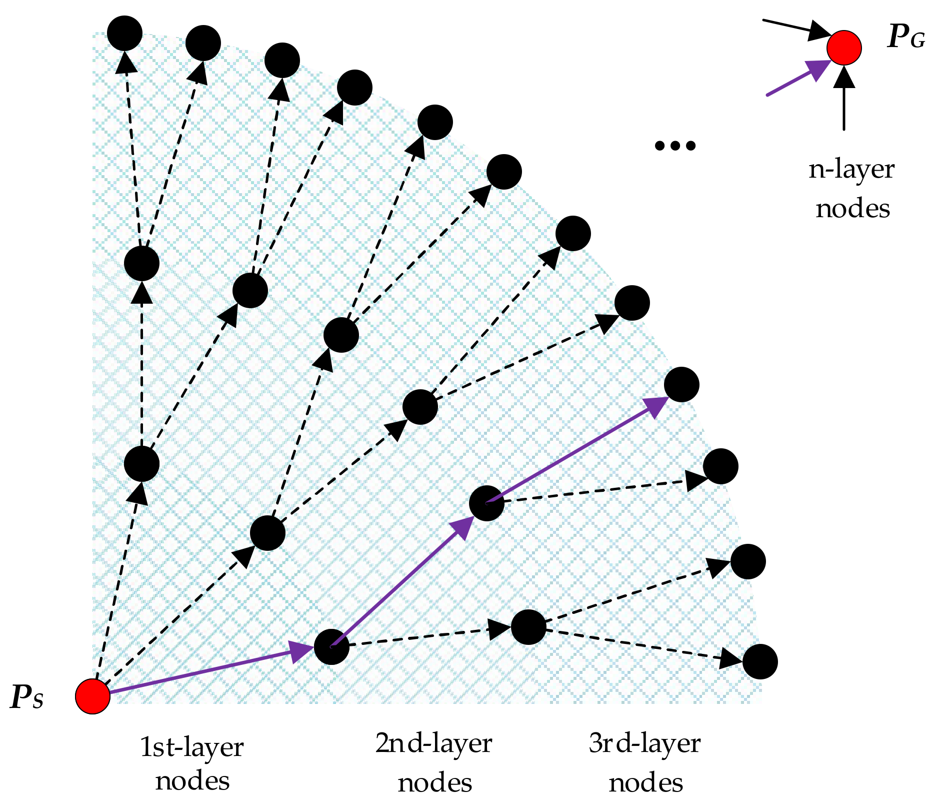
The node extension method connects the current node to its surrounding nodes in the topology graph M. The node extension method is shown in Figure 9. The start node is extended to a feasible connected node according to the connectivity matrix. If the connection path between and is feasible, a candidate node set Q is generated. The optimized node with the lowest cost is searched in the Q set, expanded to the connected nodes around it, and then the new extended node is added to set Q, until it extends to the goal node .
In the process of node extension, for the new extension nodes, the extension cost evaluation function is used to evaluate the extension cost from the parent node to the next node using weighted calculation, as shown in the formula
where is the extension cost from the parent node to node , and is the extension cost from node to . , , and are low-risk weight coefficient, high-risk weight coefficient, safe-weight coefficient and distance weight coefficient, respectively. The heuristic function is shown in the formula:
where is the heuristic cost evaluation function between the new extension node and the goal node , is the barrier weight coefficient, and , and are the heuristic barrier cost, heuristic distance cost and heuristic safe cost of node in the heuristic cost evaluation matrix, respectively.
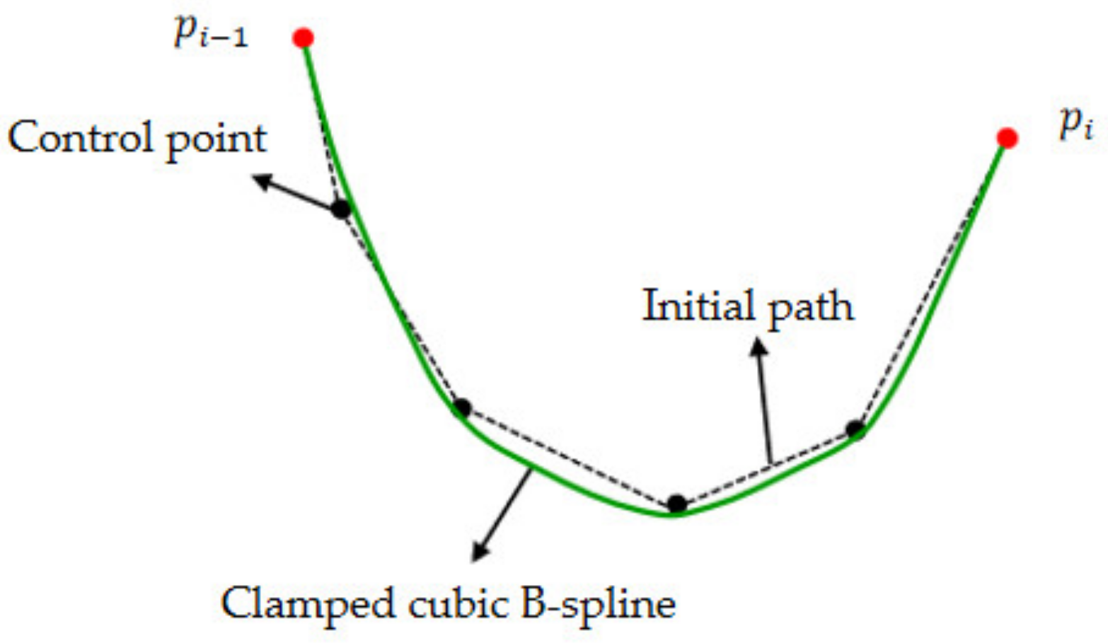
After the optimized path nodes are connected sequentially, the vehicle motion trajectory contains multi-segment polylines. Because the trajectory has hard inflection nodes, it cannot meet the requirements of vehicle kinematic constraints. In this paper, the clamped cubic B-spline smoothing method is used to optimize the trajectory of path planning; as shown in Figure 10, the black dotted line is the initial path from to , while the green curve is the result of smoothing.
3. Simulation Experiments and Discussion
3.1. Experimental Setting
3.2. Mobility Prediction Results
According to Equations (8) to (10), and the UGV parameters given in Table 1, the MI index of the UGV is 67.9, so VCI1 is 389.4 kN/m2 and VCI50 is 534.1 kN/m2. The soil types in this terrain are mainly divided into sandy loam, clayey soil, lean clay and upland sandy, as illustrated in Table 2.
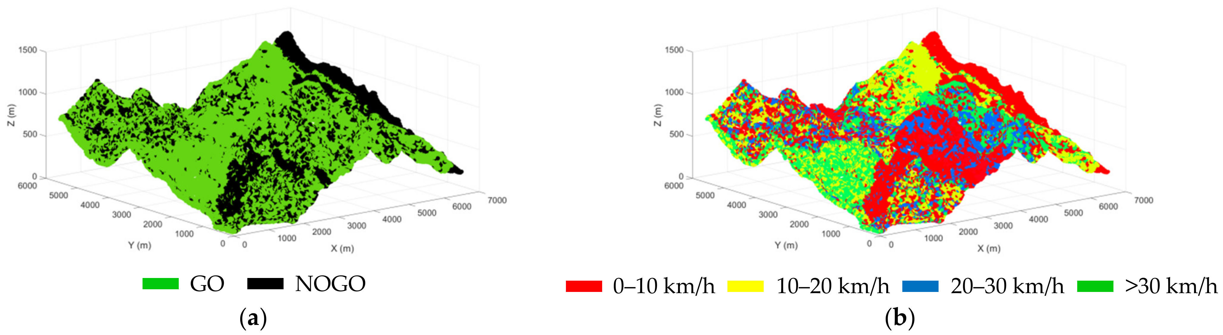
Recall that the 3D terrain model we created is a multi-dimensional model containing elevation data, soil type data (soil strength values, CI), slope values and land use data. Therefore, according to the comparison between the calculated VCI and the CI of each area, the area with a CI less than VCI1 is defined as the NOGO area. According to the obtained slope map in Figure 5, combined with the limitations of the vehicle kinematic model, if the slope value exceeds the maximum pitch angle or roll angle of the UGV, it is then determined as a NOGO area. Additionally, based on land use data, the areas covered by water and forests are also defined as NOGO areas, while the rest are GO areas. Thus, a GO/NOGO map is finally generated, as shown in Figure 12a. In this terrain, the GO areas account for 71% and the NOGO areas account for 29%. Combined with the slope value and the soil parameters in Table 1, the maximum attainable speed of the UGV in each area can be obtained using Equation (18). As a result, the maximum attainable speed distribution map of the UGV can be obtained, as shown in Figure 12b. The maximum speed that the UGV can reach is 32.4 km/h, and the average speed is 9.5 km/h.
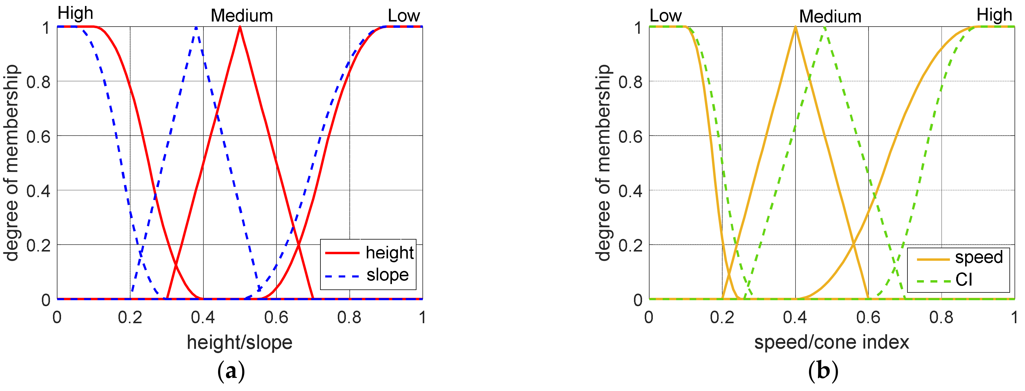
The quantification method of mobility results adopts the fuzzy inference described above; three states are defined for the three independent evaluation indexes, namely “low”, “medium” and “high”, to make the final result more accurate. These are combined with the above determination for NOGO areas, with four states being defined for the mobility cost, namely, “NOGO area”, “high-risk area”, “low-risk area” and “safe area”. Reviewing the previous section, the factors affecting mobility are summarized as the maximum attainable speed of the UGV, CI, terrain slope and height. When it comes to the fuzzy rule setting, this study references the expert rules for off-road vehicles in off-road terrain evaluation studies, such as the slope being defined as high, if in the range of 0°–8°, medium 5°–15°, and low 10°–30° [31]. Similarly, terrain height is defined as high if in the range of 0–300 m, medium 200–600 m, and low if greater than 500 m [32]. Under off-road traversing conditions, the vehicle speed is defined as low, if in the range of 0–15 km/h, medium 10–30 km/h, and high 20–40 km/h [28]. By comparing the calculated VCI1 and VCI50 to the CI, CI is defined as low if in the range of 0–500 kN/m2, medium 400–700 kN/m2, and high if greater than 700 kN/m2 (See Appendix B for details of the specific rules setting). When determining the membership function, we normalize the input data, then use the S-type membership function, triangular membership function and Z-type membership function to express the fuzzy rules, as shown in Figure 13.
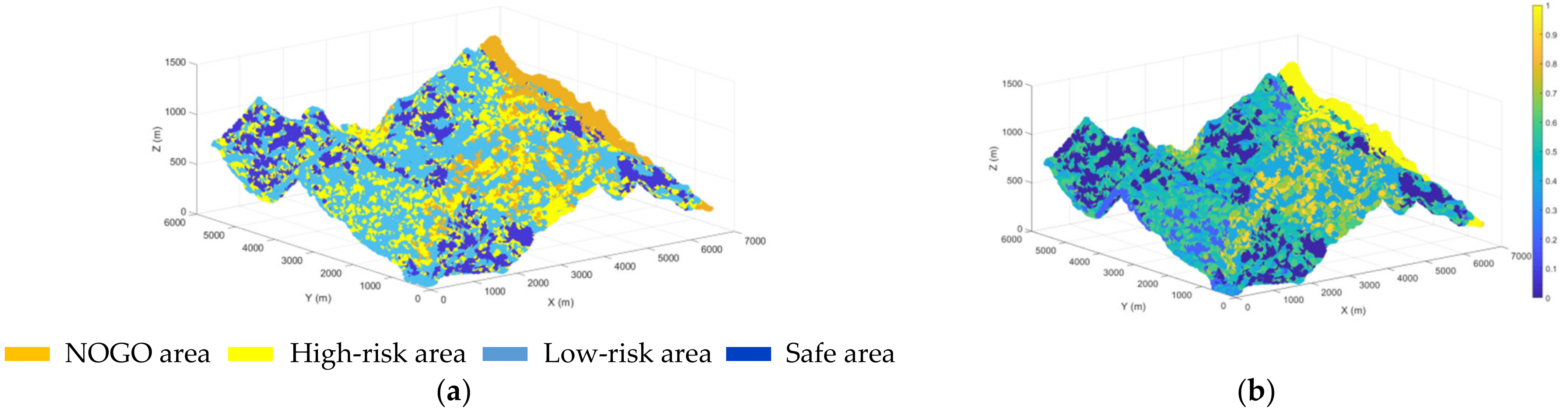
The defuzzification process uses the “Max–min” criterion proposed in Section 2.3. After defuzzification, the global terrain is divided into four categories, as shown in Figure 14a. The mobility cost evaluation result is also expressed as the distribution of [0, 1], and the closer to 1, the worse the mobility, as shown in Figure 14b.
3.3. Path Generation Results
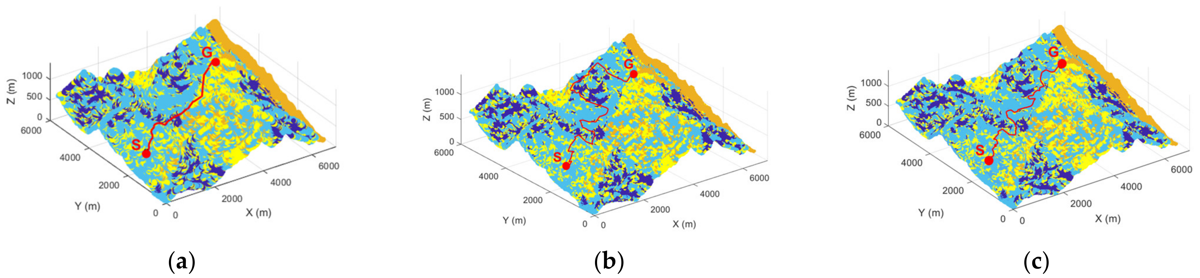
After obtaining the mobility cost results, the improved A* algorithm described above is used for global path planning (min-mobility cost route). We also compare two other algorithms, the traditional A* algorithm for searching the shortest route (min-distance route), and the A* algorithm with the consideration of the terrain profile (min-slope route) [33], as shown in Figure 15.
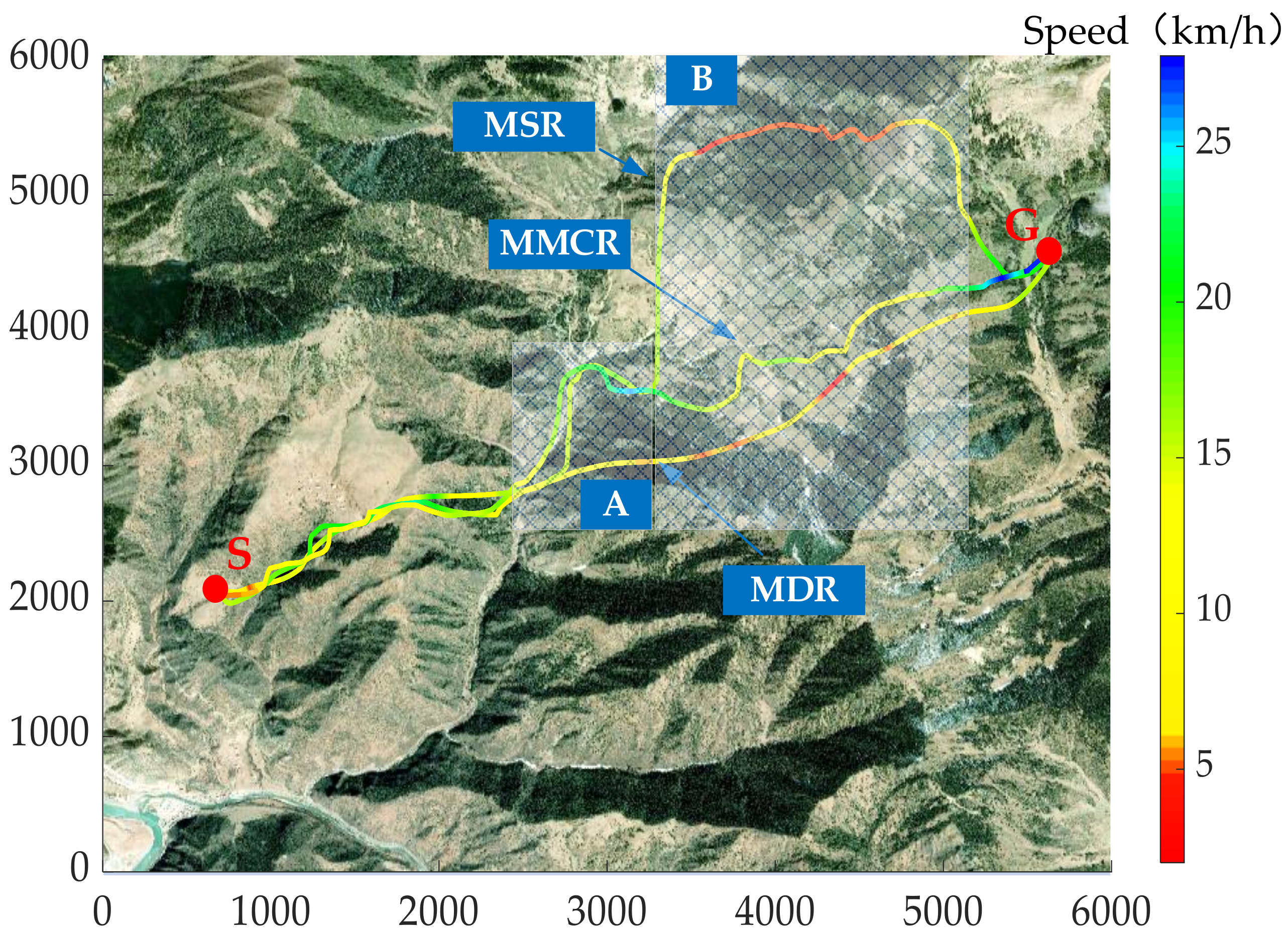
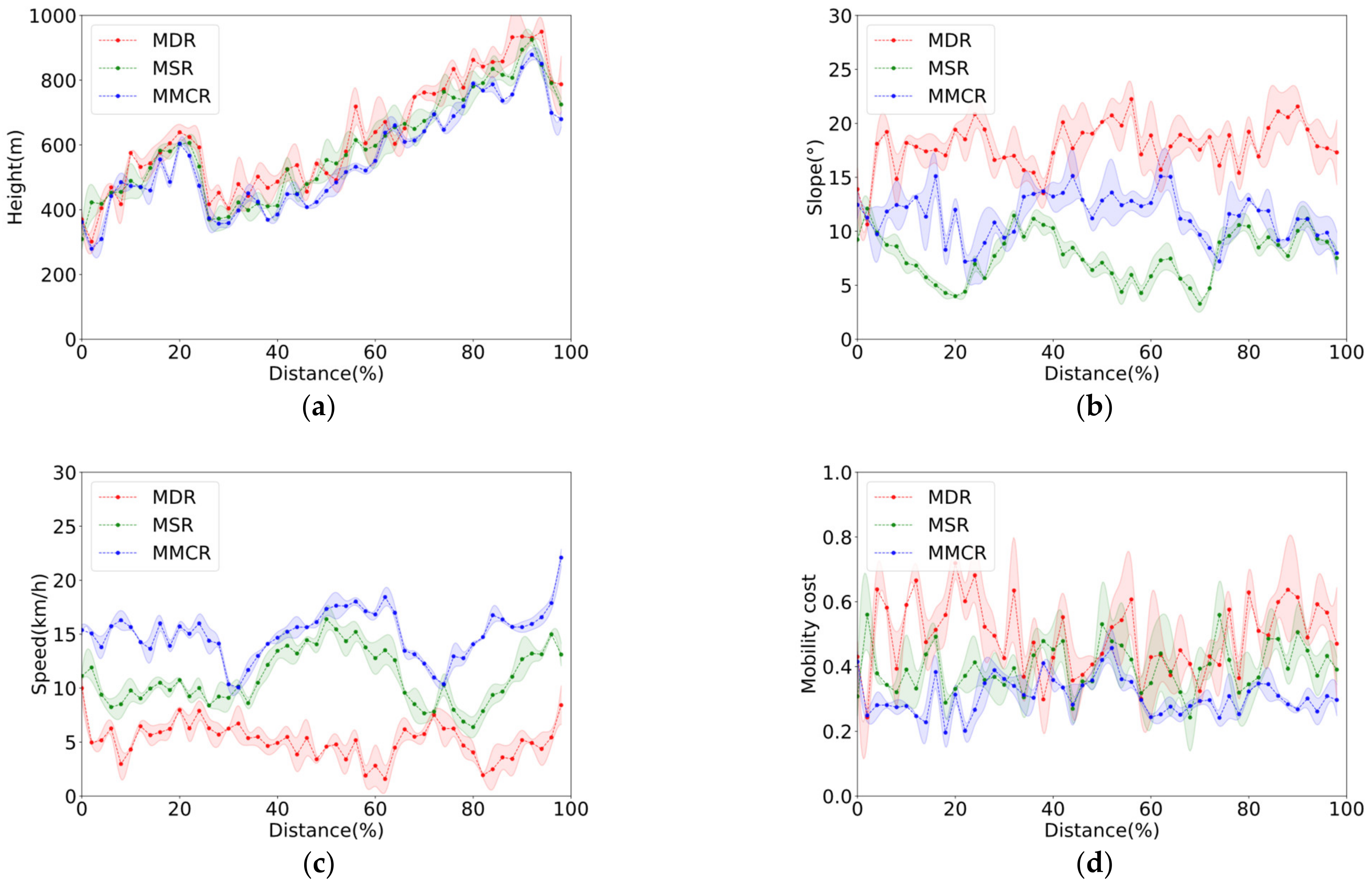
The final experimental result shows that the three path planning strategies generate three global routes, namely, MDR (min-distance route), MSR (min-slope route) and MMCR (min-mobility cost route), as given in Figure 16. To intuitively evaluate the routes generated at different costs, each route node is stored and statistically analyzed. All routes are normalized and segmented in Table 3 to show the average indicators of the UGV in different route segments, and the detailed comparison of the data is shown in Figure 17. After ignoring the NOGO areas, MDR adopts the planning strategy of the shortest route. The comparison of experimental results also proves that this route is the shortest. However, only the distance factor is considered, and the influence of slope and soil strength on vehicle mobility are ignored. The route has the highest average slope (20.9°), the highest height (628.8 m), the lowest average speed (5.3 km/h) and the longest traversing time (1.47 h). Combined with the abovementioned fuzzy rules, the MDR is classified as “high risk”. MSR adopts the planning strategy of the slowest route. It is obvious that the route has the smallest average slope (8.5°); because only the influence of slope is considered in the cost function, the slowest route leads to the longest path length (11,670 m). Simultaneously, when searching for the slowest route, it inevitably selects areas with low soil strength, resulting in an increase in traversing resistance and reduced average speed (11.5 km/h). Combined with fuzzy rules, MSR is classified as “low risk”. Conversely, the minimum mobility cost planning strategy proposed in this paper comprehensively considers the influence of terrain. On this basis, the terrain points with higher speed are searched as the route nodes. Therefore, this route has the highest average speed (13.8 km/h) and the least traversing time (0.62 h), and its fuzzy result is “low risk”.
In addition, the computer execution time for the three methods in Matlab shows the longest to be MSR, which takes 75 min, followed by MDR, which takes 44 min, whereas MCCR combines the characteristics of the sampling algorithm and, therefore, takes the least time, less than 4 min; these experiments were run on a general-purpose computer (Intel Core i7 3 GHz,16 MB RAM).
In order to further prove the effectiveness of the algorithm in this paper, the generated routes are extracted and compared with regions A and B, with a large difference in fitting degree, as shown in Figure 18.
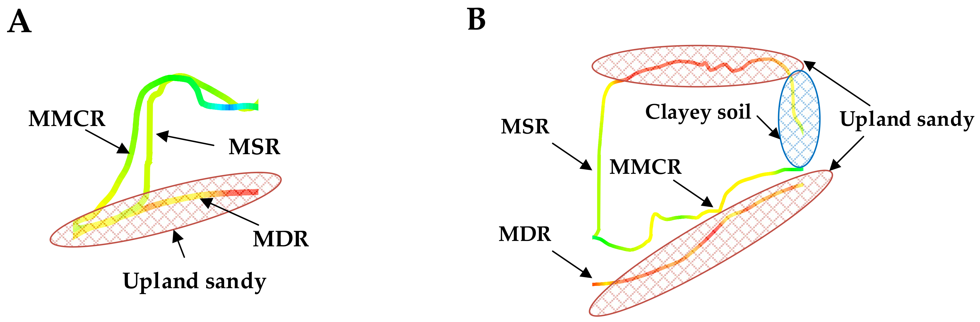
Region A has two types of soil, lean clay (CI = 1070.5 kN/m2, 77%) and upland sandy (CI = 528.5 kN/m2, 23%), while the average slope value in this area is 15.6° with a standard deviation of 4.2. The comparison results of the three routes are shown in Table 4.
In region A, MDR only considers distance cost, resulting in traversing areas with low soil strengths and high slopes, so it has the lowest average speed (4.8 km/h) and the longest traversal time. In the MSR search process, only the slope cost is considered, and the result satisfies the requirement of searching for the slowest route; however, this process also produces the longest route and a route with low soil strength. MMCR proposed in this paper, and which considers the comprehensive factors (mobility cost), avoids the soft soil areas well, so that it can search along the lean clay area; this route has the best mobility, with the highest average speed (13.3 km/h) and the lowest time (0.17 h). It also has a smoother route by using the B-spline curve.
In the case of the large terrain relief in region B (mean slope value of 21.1°, standard deviation of 6.7), the soil contains lean clay (CI = 1070.5 kN/m2, 56%), upland sandy (CI = 528.5 kN/m2, 27%) and clayey soil (CI = 732.5 kN/m2, 17%); the results of the three planning strategies are shown in Table 5.
In region B, MDR still searches for the shortest route within the upland sandy; its average speed is further limited (3.9 km/h) due to the increase in terrain undulation; although its route distance is the shortest, it takes the longest time (0.74 h). Due to the large change of slope, MSR only pursues a gentler route and also increases traversing distance. Meanwhile, part of the route enters the area of upland sandy and clayey soil with relatively low soil strength, which leads to a lower average speed. MMCR can avoid this situation well on the basis of the mobility cost quantification method, while being able to find a faster route on the high strength soils (average speed 12.1 km/h, traversing time 0.28 h).
4. Conclusions and Future Work
In this paper, a mobility prediction-based global path planning method for UGVs is proposed. The experimental results show that the proposed method, MMCR, can effectively generate a more feasible, efficient and safer route when considering the mobility cost. It is worth noting that the current path-planning technologies usually rely on terrain modeling by the UGV’s own sensory devices, which can build a more detailed terrain model, but the data storage volume required is huge and the data parsing method is relatively complex. Sensing the surrounding environment in the actual unknown off-road terrain is likely to cause the risk of failure of the unmanned equipment. This paper proposed an effective method to reconstruct 3D off-road terrain by fusing multi-source remote sensing data based on the Kriging interpolation method. Also based on terramechanics and fuzzy inference, the effect of soil deformation on the UGV is considered to reduce the risk of obstruction. In summary, this paper provides an effective and safe reference method for UGVs to perform off-road tasks. The method is not only applicable to the terrain selected in this paper, but also applicable to other terrains, so it is generalized, and has a certain value in engineering applications.
Future work will focus on several limitations of this study. (1) The limitation of this study is that the attitude change of the vehicle during the driving process is not taken into account; therefore, to obtain more accurate and more informative mobility prediction results, discrete element or finite element techniques will be considered for modeling the soil and coupling the soil model with the vehicle model for simulation. Although several techniques for coupled simulation have been proposed [34,35], these approaches are, nevertheless, time-consuming when predicting mobility over large areas. To obtain mobility prediction results efficiently, it is necessary to combine these methods with machine learning algorithms. (2) On the other hand, there are perceptual errors in satellite remote sensing data and interpolation errors generated using terrain interpolation methods, as well as spatial variability in physical soil properties (water content, season, etc.); all of these may lead to uncertain results of mobility prediction. Therefore, how to reduce or quantify the uncertainty of mobility prediction will be another future research direction.
Author Contributions
Conceptualization, C.H., R.N. and B.Y.; methodology, C.H.; formal analysis, B.Y.; investigation, C.H. and B.Y.; resources, B.Y.; data curation, X.Z.; writing—original draft preparation, C.H.; writing—review and editing, C.H., B.Y. and X.Z.; visualization, C.H., R.B. and S.Z.; supervision, B.Y.; project administration, B.Y.; funding acquisition, B.Y. All authors have read and agreed to the published version of the manuscript.
Funding
This work was supported by Youth Innovation Promotion Association of CAS (Y2021115).
Institutional Review Board Statement
Not applicable.
Informed Consent Statement
Not applicable.
Data Availability Statement
The satellite map and digital elevation model are downloaded on the geospatial data cloud website, http://www.gscloud.cn/sources (accessed on 26 April 2021); soil type distribution data and land use data can be obtained from the National Earth System Science Data Center website, http://www.geodata.cn/data (accessed on 7 July 2021). Some data presented in this study are available on request from the corresponding author. The data are not publicly available due to the confidentiality clause of some projects.
Conflicts of Interest
The authors declare no conflict of interest.
Appendix A
Appendix A.1. Projection of Each Data Type
We project the soil type distribution data and land use data onto the corresponding 3D terrain model, respectively, and the results are shown in Figure A1. In this research, we define water areas and forest lands as NOGO areas. According to the comparison between VCI and CI calculated above, sandy loam is defined as a NOGO area. In particular, since the CI of lean clay is between VCI1 and VCI50, these areas are relatively difficult to traverse.
Figure A1.
Data projection results. (a) The projection results of soil type distribution data. (b) The projection results of land use data.
Figure A1.
Data projection results. (a) The projection results of soil type distribution data. (b) The projection results of land use data.

Appendix A.2. The Slope Map Calculation Process
According to the interpolated 3D terrain model, the slope value of each point in the data can be calculated, as shown in Figure A2; we used the 3 × 3 moving window to traverse the whole point and calculated the slope value of each point. The calculation formula of the slope value of each point is
where (i =1, …, 8) are the elevation values of eight points near the calculated point h and d is the resolution size.
Figure A2.
The calculation method of slope in 3 × 3 grid traversal window.

Appendix B
The input of fuzzy rules in this paper comprises four types (slope, height, CI and speed) and the output is Mobility, each with three states as “low (high-risk area)”, “medium (low-risk area)” and “high (safe area)”, as shown in the Table A1, so there are 81 fuzzy inference rules, as shown in the Table A2. To reduce the risk for the UGV in the off-road environment, a fuzzy inference rule strategy, which is on the conservative side, is used. The distribution of mobility state results: 26 for “L”,38 for “M”, and 17 for “H”.

Table A1.
Fuzzy state of each variable.
| Variable | Fuzzy State | ||
|---|---|---|---|
| Slope | L1 | M1 | H1 |
| Height | L2 | M2 | H2 |
| CI | L3 | M3 | H3 |
| Speed | L4 | M4 | H4 |
| Mobility | L | M | H |
Table A2.
Fuzzy inference rules.
| If L1 and L2 and L3 and L4 then L; | If M1 and M2 and M3 and H4 then H; |
| If L1 and L2 and L3 and M4 then L; | If M1 and M2 and H3 and L4 then M; |
| If L1 and L2 and L3 and H4 then L; | If M1 and M2 and H3 and M4 then M; |
| If L1 and L2 and M3 and L4 then L; | If M1 and M2 and H3 and H4 then H; |
| If L1 and L2 and M3 and M4 then L; | If M1 and H2 and L3 and L4 then L; |
| If L1 and L2 and M3 and H4 then L; | If M1 and H2 and L3 and M4 then M; |
| If L1 and L2 and H3 and L4 then L; | If M1 and H2 and L3 and H4 then M; |
| If L1 and L2 and H3 and M4 then L; | If M1 and H2 and M3 and L4 then M; |
| If L1 and L2 and H3 and H4 then M; | If M1 and H2 and M3 and M4 then H; |
| If L1 and M2 and L3 and L4 then L; | If M1 and H2 and M3 and H4 then H; |
| If L1 and M2 and L3 and M4 then L; | If M1 and H2 and H3 and L4 then M; |
| If L1 and M2 and L3 and H4 then L; | If M1 and H2 and H3 and M4 then H; |
| If L1 and M2 and M3 and L4 then L; | If M1 and H2 and H3 and H4 then H; |
| If L1 and M2 and M3 and M4 then M; | If H1 and L2 and L3 and L4 then L; |
| If L1 and M2 and M3 and H4 then M; | If H1 and L2 and L3 and M4 then L; |
| If L1 and M2 and H3 and L4 then L; | If H1 and L2 and L3 and H4 then M; |
| If L1 and M2 and H3 and M4 then M; | If H1 and L2 and M3 and L4 then L; |
| If L1 and M2 and H3 and H4 then H; | If H1 and L2 and M3 and M4 then M; |
| If L1 and H2 and L3 and L4 then L; | If H1 and L2 and M3 and H4 then M; |
| If L1 and H2 and L3 and M4 then M; | If H1 and L2 and H3 and L4 then M; |
| If L1 and H2 and L3 and H4 then M; | If H1 and L2 and H3 and M4 then M; |
| If L1 and H2 and M3 and L4 then L; | If H1 and L2 and H3 and H4 then M; |
| If L1 and H2 and M3 and M4 then M; | If H1 and M2 and L3 and L4 then L; |
| If L1 and H2 and M3 and H4 then M; | If H1 and M2 and L3 and M4 then M; |
| If L1 and H2 and H3 and L4 then M; | If H1 and M2 and L3 and H4 then M; |
| If L1 and H2 and H3 and M4 then M; | If H1 and M2 and M3 and L4 then M; |
| If L1 and H2 and H3 and H4 then H; | If H1 and M2 and M3 and M4 then M; |
| If M1 and L2 and L3 and L4 then L; | If H1 and M2 and M3 and H4 then H; |
| If M1 and L2 and L3 and M4 then L; | If H1 and M2 and H3 and L4 then M; |
| If M1 and L2 and L3 and H4 then L; | If H1 and M2 and H3 and M4 then H; |
| If M1 and L2 and M3 and L4 then L; | If H1 and M2 and H3 and H4 then H; |
| If M1 and L2 and M3 and M4 then M; | If H1 and H2 and L3 and L4 then M; |
| If M1 and L2 and M3 and H4 then M; | If H1 and H2 and L3 and M4 then M; |
| If M1 and L2 and H3 and L4 then L; | If H1 and H2 and L3 and H4 then H; |
| If M1 and L2 and H3 and M4 then M; | If H1 and H2 and M3 and L4 then M; |
| If M1 and L2 and H3 and H4 then M; | If H1 and H2 and M3 and M4 then H; |
| If M1 and M2 and L3 and L4 then L; | If H1 and H2 and M3 and H4 then H; |
| If M1 and M2 and L3 and M4 then M; | If H1 and H2 and H3 and L4 then H; |
| If M1 and M2 and L3 and H4 then M; | If H1 and H2 and H3 and M4 then H; |
| If M1 and M2 and M3 and L4 then M; | If H1 and H2 and H3 and H4 then H |
| If M1 and M2 and M3 and M4 then M; |
References
- Zhu, P.; Ferrari, S.; Morelli, J.; Linares, R.; Doerr, B. Scalable Gas Sensing, Mapping, and Path Planning via Decentralized Hilbert Maps. Sensors 2019, 19, 1524. [Google Scholar] [CrossRef] [PubMed] [Green Version]
- Quann, M.; Ojeda, L.; Smith, W.; Rizzo, D.; Castanier, M.; Barton, K. Off-road Ground Robot Path Energy Cost Prediction Through Probabilistic Spatial Mapping. J. Field Robot. 2019, 37, 421–439. [Google Scholar] [CrossRef]
- Paden, B.; Cap, M.; Yong, S.Z.; Yershov, D.; Frazzoli, E. A Survey of Motion Planning and Control Techniques for Self-driving Urban Vehicles. IEEE Trans. Intell. Veh. 2016, 1, 133–155. [Google Scholar] [CrossRef] [Green Version]
- Algfoor, Z.A.; Sunar, M.S.; Abdullah, A. A New Weighted Path Finding Algorithms to Reduce The Search Time on Grid Maps. Expert Syst. Appl. 2017, 71, 319–331. [Google Scholar] [CrossRef]
- Norhafezah, K.; Nurfadzliana, A.H.; Megawati, O. Simulation of Municipal Solid Waste Route Optimization by Dijkstra’s Algorithm. J. Fundam. Appl. Sci. 2018, 9, 732–747. [Google Scholar] [CrossRef] [Green Version]
- Alazzam, H.H.; Abualghanam, O.; Sharieh, A.A. Best Path in Mountain Environment Based on Parallel A* Algorithm and Apache Spark. J. Supercomput. 2021, 78, 5075–5094. [Google Scholar] [CrossRef]
- Shi, J.; Liu, C.; Xi, H. Improved D* Path Planning Algorithm Based on CA Model. J. Electron. Meas. Instrum. 2016, 30, 30–37. [Google Scholar]
- Wang, Z.; Zeng, G.; Huang, B.; Fang, Z. Global Optimal Path Planning for Robots with Improved A* Algorithm. Comput. Appl. 2019, 39, 2517–2522. [Google Scholar]
- Guruji, A.K.; Agarwal, H.; Parsediya, D.K. Time Efficient A Algorithm for Robot Path Planning. Procedia Technol. 2016, 23, 144–149. [Google Scholar] [CrossRef] [Green Version]
- Duan, S.; Wang, Q.; Han, X. Improved A-star Algorithm for Safety Insured Optimal Path with Smoothed Corner Turns. J. Mech. Eng. 2020, 56, 205–215. [Google Scholar]
- Li, Y.; Cui, R.; Li, Z.; Xu, D.M. Neural Network Approximation Based Near-optimal Motion Planning with Knodynamic Constraints Using RRT. IEEE Trans. Ind. Electron. 2018, 65, 8718–8729. [Google Scholar] [CrossRef]
- Xu, Z.; Deng, D.; Shimada, K. Autonomous UAV Exploration of Dynamic Environments via Incremental Sampling and Probabilistic Roadmap. IEEE Robot. Autom. Lett. 2021, 6, 2729–2736. [Google Scholar] [CrossRef]
- Gammell, J.D.; Barfoot, T.D.; Srinivasa, S.S. Informed Sampling for Asymptotically Optimal Path Planning. IEEE Trans. Robot. 2018, 34, 966–984. [Google Scholar] [CrossRef] [Green Version]
- Dolgov, D.; Thrun, S.; Montemerlo, M. Path Planning for Autonomous Vehicles in Unknown Semi-structured Environments. Int. J. Robot. Res. 2010, 29, 485–501. [Google Scholar] [CrossRef]
- Zaid, T.; Qureshi, A.H.; Yasar, A.; Nawaz, R. Potentially Guided Bidirectionalized RRT* for Fast Optimal Path Planning in Cluttered Environments. Robot. Auton. Syst. 2018, 108, 13–27. [Google Scholar]
- Park, B.; Choi, J.; Chung, W.K. Incremental Hierarchical Roadmap Construction for Efficient Path Planning. ETRI J. 2018, 40, 458–470. [Google Scholar] [CrossRef]
- Cheng, C.Q.; Hao, X.Y.; Li, J.S. Global dynamic path planning based on improved A* algorithm and dynamic window method. J. Xi’an Jiao Tong Univ. 2017, 51, 137–143. [Google Scholar]
- Hu, J.; Hu, Y.; Lu, C. Integrated Path Planning for Unmanned Differential Steering Vehicles in Off-Road Environment with 3D Terrains and Obstacles. IEEE Trans. Intell. Transp. Syst. 2021, 18, 1–11. [Google Scholar] [CrossRef]
- Gonzalez, R.; Jayakumar, P.; Iagnemma, K. Stochastic Mobility Prediction of Ground Vehicles over Large Spatial Regions: A Geostatistical Approach. Auton. Robot. 2017, 41, 311–331. [Google Scholar] [CrossRef]
- Jiang, C.; Hu, Z.; Mourelatos, Z.P.; Gorsich, D.; Jayakumar, P.; Fu, Y.; Majcher, M. R2-RRT*: Reliability-Based Robust Mission Planning of Off-Road Autonomous Ground Vehicle Under Uncertain Terrain Environment. IEEE Trans. Autom. Sci. Eng. 2022, 19, 1030–1046. [Google Scholar] [CrossRef]
- Lv, T.; Feng, M. A Smooth Local Path Planning Algorithm Based on Modified Visibility Graph. Mod. Phys. Lett. B 2017, 31, 174–184. [Google Scholar] [CrossRef]
- Liu, J.; Ji, J.; Ren, Y.; Huang, Y.J.; Wang, H. Path Planning for Vehicle Active Collision Avoidance Based on Virtual Flow Field. Int. J. Automot. Technol. 2021, 22, 1557–1567. [Google Scholar] [CrossRef]
- Choi, K.K.; Jayaktumar, P.; Funk, M.; Gatul, N.; Wasfy, T.M. Framework of Reliability-Based Stochastic Mobility Map for Next Generation NATO Reference Mobility Model. J. Comput. Nonlinear Dyn. 2018, 14, 132–143. [Google Scholar] [CrossRef] [Green Version]
- Gonzalez, R.; Jayakumar, P.; Iagnemma, K. An Efficient Method for Increasing the Accuracy of Mobility Maps for Ground Vehicles. J. Terramech. 2016, 68, 23–35. [Google Scholar] [CrossRef]
- Wong, J.Y.; Jayakumar, P.; Toma, E. A Review of Mobility Metrics for Next Generation Vehicle Mobility Models. J. Terramech. 2020, 87, 11–20. [Google Scholar] [CrossRef]
- Wong, J.Y.; Jayakumar, P.; Toma, E. Comparison of Simulation Models NRMM and NTVPM for Assessing Military Tracked Vehicle Cross-country Performance. J. Terramech. 2018, 80, 31–48. [Google Scholar] [CrossRef]
- Wasfy, T.M.; Jayakumar, P. Next-generation NATO Reference Mobility Model Complex Terramechanics—Part 2: Requirements and Prototype. J. Terramech. 2021, 5, 59–79. [Google Scholar] [CrossRef]
- George, A.K.; Singh, H.; Dattathreya, M.S.; Meitzler, T.J. A Fuzzy Simulation Model for Military Vehicle Mobility Assessment. Adv. Fuzzy Syst. 2017, 23, 179–191. [Google Scholar] [CrossRef] [Green Version]
- Huang, J.; Ri, M.; Wu, D.R.; Ri, S. Interval Type-2 Fuzzy Logic Modeling and Control of a Mobile Two-Wheeled Inverted Pendulum. IEEE Trans. Fuzzy Syst. 2018, 26, 2030–2038. [Google Scholar] [CrossRef]
- Yang, F. Research on Key Techniques of Vehicle Trafficability Based on Wheel Force Test. Ph.D. Thesis, Southeast University, Nanjing, China, May 2016. [Google Scholar]
- Wong, J.Y. Theory of Ground Vehicles, 4th ed.; Machine Press: Beijing, China, 2018; pp. 210–268. [Google Scholar]
- Sonker, R.; Dutta, A. Adding Terrain Height to Improve Model Learning for Path Tracking on Uneven Terrain by a Four-Wheel Robot. IEEE Robot. Autom. Lett. 2020, 6, 239–246. [Google Scholar] [CrossRef]
- Zhang, K.; Yang, Y.; Fu, M.; Wang, M.L. Traversability Assessment and Trajectory Planning of Unmanned Ground Vehicles with Suspension Systems on Rough Terrain. Sensors 2019, 19, 4372. [Google Scholar] [CrossRef] [PubMed] [Green Version]
- Mechergui, D.; Jayakumar, P. Efficient Generation of Accurate Mobility Maps Using Machine Learning Algorithms. J. Terramech. 2020, 88, 53–63. [Google Scholar] [CrossRef]
- Yang, P.; Zang, M.; Zeng, H. An efficient 3D DEM-FEM Contact Detection Algorithm for Tire-sand Interaction. Powder Technol. 2020, 360, 1102–1116. [Google Scholar] [CrossRef]
Figure 1.
The method framework.

Figure 2.
Multi source data with a resolution of 30 m in the target area. (a) Satellite imagery, (b) DEM (elevation), (c) Soil type distribution data, (d) Land use data.
Figure 2.
Multi source data with a resolution of 30 m in the target area. (a) Satellite imagery, (b) DEM (elevation), (c) Soil type distribution data, (d) Land use data.

Figure 3.
3D terrain model.

Figure 4.
The reconstructed terrain map and slope map. (a) Terrain reconstruction with a resolution of 10 m using the ordinary Kriging method, (b) Slope map of 3D terrain.
Figure 4.
The reconstructed terrain map and slope map. (a) Terrain reconstruction with a resolution of 10 m using the ordinary Kriging method, (b) Slope map of 3D terrain.

Figure 5.
Patterns of the tire on different soil strengths, is tire inflation pressure, is tire stiffness pressure, is the support force of the lowest point of the tire, is the static settlement of the tire, L is the deformation length of the tire. (a) Rigid mode, where: , (b) Elastic mode, where .
Figure 5.
Patterns of the tire on different soil strengths, is tire inflation pressure, is tire stiffness pressure, is the support force of the lowest point of the tire, is the static settlement of the tire, L is the deformation length of the tire. (a) Rigid mode, where: , (b) Elastic mode, where .

Figure 6.
Block diagram of the proposed mobility quantification method. In this case, the maximum attainable speed of the UGV and multiple terrain factors (slope, height and soil) are taken as the input sets. In the fuzzy inference process, firstly, the fuzzifier converts the numerical value obtained from the input data into fuzzy sets. Which is, the input variables are represented in terms of their degree of membership for different membership functions. Secondly, the rules use “If–then” structure to relate the input sets to the output sets. Thirdly, the inference engine takes the input sets and decides which rules should be used from the rule base and creates the output sets. Finally, the defuzzifier takes the fuzzy output sets created by the inference engine and generates the output results (area classification and the mobility cost).

Figure 7.
Schematic diagram of the membership function.

Figure 8.
Node extension diagram. (a) Connectivity matrix diagram, taking nodes , and as an example, since the connecting line between and passes through the NOGO area, so , are “0”, , , are also “0”; on the contrary, , , and are “1”, (b) Extended low risk cost matrix diagram, dividing the connecting line between and evenly into n child nodes, accumulating the cost value of the nodes contained in , similarly, calculating the other nodes in the same way, (c) Extension distance cost matrix diagram, (d) Heuristic barrier cost diagram, the current nodes , and are connected to the goal node , and each connecting line is discretized into n child nodes, which are accumulated and calculated, respectively, to obtain the heuristic cost of each line segment.

Figure 9.
Nodes extension process.

Figure 10.
Clamped cubic B-spline interpolation.

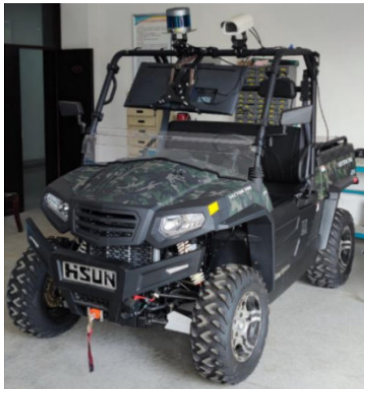
Figure 11.
The experimental UGV.

Figure 12.
Distribution map of GO/NOGO and maximum attainable speed. (a) GO/NOGO map, (b) Maximum attainable speed map.
Figure 12.
Distribution map of GO/NOGO and maximum attainable speed. (a) GO/NOGO map, (b) Maximum attainable speed map.

Figure 13.
Membership of fuzzy rules. (a) Degree of membership of the height and slope, (b) Degree of membership of the speed and CI.
Figure 13.
Membership of fuzzy rules. (a) Degree of membership of the height and slope, (b) Degree of membership of the speed and CI.

Figure 14.
Fuzzy inference results. (a) Fuzzy inference result for four categories: NOGO area, high-risk area, low-risk area and safe area, (b) Fuzzy inference result for the mobility cost of [0, 1].
Figure 14.
Fuzzy inference results. (a) Fuzzy inference result for four categories: NOGO area, high-risk area, low-risk area and safe area, (b) Fuzzy inference result for the mobility cost of [0, 1].

Figure 15.
Comparison of the three routes, the global path planning algorithm that considers mobility as a function of cost (min-mobility cost route), considers distance (min-distance route), and considers terrain profile (min-slope route). (a) Min-distance route, (b) Min-slope route, (c) Min-mobility cost route.

Figure 16.
Comparison of maximum attainable speed under three path planning strategies on satellite map, A and B are the regions with large deviations in the routes, respectively.
Figure 16.
Comparison of maximum attainable speed under three path planning strategies on satellite map, A and B are the regions with large deviations in the routes, respectively.

Figure 17.
Comparison of various mobility indicators of the planned routes. (a) Height comparison curve, (b) Slope comparison curve, (c) Maximum attainable speed comparison curve, (d) Mobility cost comparison curve. By counting the elevation, slope and velocity of each node, the first three sets of curves show that MMCR has a clear advantage over the other two planning strategies, while its data have a small standard deviation (the standard deviation is represented by the envelope area on both sides of the curve), which also corresponds to the trend in the mobility cost of each node of curve (d). Therefore, it further proves the superiority of the path planning strategy that considers the smallest integrated mobility cost.

Figure 18.
Comparison of the three routes in the two regions. In region (A), the red grid area is upland sandy area, except for lean clay area. In region (B), the red grid areas are upland sandy areas and the blue grid area is upland sandy area, except for lean clay area.
Figure 18.
Comparison of the three routes in the two regions. In region (A), the red grid area is upland sandy area, except for lean clay area. In region (B), the red grid areas are upland sandy areas and the blue grid area is upland sandy area, except for lean clay area.

Table 1.
Parameters of the UGV model.
| Parameters | Gross Mass/kg | Clearance/m | Number of Axles | Number of Tires | Tire Load/N | Tire Width/m | Tire Radius/m | Engine Power/kW |
|---|---|---|---|---|---|---|---|---|
| Value | 1242 | 0.45 | 2 | 4 | 3200 | 0.40 | 0.51 | 262 |
Table 2.
Soil characteristic parameters.
| Soil Type | Moisture Content (%) | Deformation Index (n) | Cohesive Force Modulus (kN/mn+1) | Internal Friction Modulus (kN/mn+2) | Sinkage (m) | Rolling Resistance (kN) | Cone Index (kN/m2) |
| Sandy loam | 26 | 0.30 | 2.79 | 141.11 | 0.51 | 18.84 | 223.40 |
| Clayey soil | 38 | 0.50 | 13.19 | 692.15 | 0.13 | 8.86 | 732.50 |
| Lean clay | 22 | 0.20 | 16.43 | 1724.69 | 0.02 | 3.11 | 1070.50 |
| Upland sandy | 51 | 1.10 | 74.60 | 2080.00 | 0.16 | 9.32 | 528.50 |
Table 3.
Summary of the three cost functions considered in this research.
| Route | Distance (m) | Average Height (m) | Average Slope (°) | Average Speed (km/h) | Average Mobility Cost | Traversal Time (h) |
|---|---|---|---|---|---|---|
| MDR | 6724 | 628.8 | 20.9 | 5.3 | 0.48 | 1.47 |
| MSR | 11,670 | 593.2 | 8.5 | 11.5 | 0.40 | 1.01 |
| MMCR | 8306 | 551.1 | 12.4 | 13.8 | 0.32 | 0.62 |
Table 4.
Comparison of the parameters of the three routes in region A.
| Route | Distance (m) | Average Height (m) | Average Slope (°) | Average Speed (km/h) | Traversal Time (h) |
|---|---|---|---|---|---|
| MDR | 1465 | 518.7 | 16.1 | 4.8 | 0.31 |
| MSR | 2734 | 563.4 | 8.8 | 8.9 | 0.30 |
| MMCR | 2267 | 500.2 | 9.1 | 13.3 | 0.17 |
Table 5.
Comparison of the parameters of the three routes in region B.
| Route | Distance (m) | Average Height (m) | Average Slope (°) | Average Speed (km/h) | Traversal Time (h) |
|---|---|---|---|---|---|
| MDR | 2890 | 708.7 | 18.3 | 3.9 | 0.74 |
| MSR | 4518 | 686.4 | 10.8 | 7.2 | 0.63 |
| MMCR | 3321 | 644.2 | 13.3 | 12.1 | 0.28 |
Publisher’s Note: MDPI stays neutral with regard to jurisdictional claims in published maps and institutional affiliations. |
© 2022 by the authors. Licensee MDPI, Basel, Switzerland. This article is an open access article distributed under the terms and conditions of the Creative Commons Attribution (CC BY) license (https://creativecommons.org/licenses/by/4.0/).
Share and Cite
MDPI and ACS Style
Hua, C.; Niu, R.; Yu, B.; Zheng, X.; Bai, R.; Zhang, S. A Global Path Planning Method for Unmanned Ground Vehicles in Off-Road Environments Based on Mobility Prediction. Machines 2022, 10, 375. https://doi.org/10.3390/machines10050375
AMA Style
Hua C, Niu R, Yu B, Zheng X, Bai R, Zhang S. A Global Path Planning Method for Unmanned Ground Vehicles in Off-Road Environments Based on Mobility Prediction. Machines. 2022; 10(5):375. https://doi.org/10.3390/machines10050375
Chicago/Turabian StyleHua, Chen, Runxin Niu, Biao Yu, Xiaokun Zheng, Rengui Bai, and Song Zhang. 2022. "A Global Path Planning Method for Unmanned Ground Vehicles in Off-Road Environments Based on Mobility Prediction" Machines 10, no. 5: 375. https://doi.org/10.3390/machines10050375
Note that from the first issue of 2016, this journal uses article numbers instead of page numbers. See further details here.