
Semi-Analytical Approach and Green’s Function Method: A Comparison in the Analysis of the Interaction of a Moving Mass on an Infinite Beam on a Three-Layer Viscoelastic Foundation at the Stability Limit—The Effect of Damping of Foundation Materials


Abstract
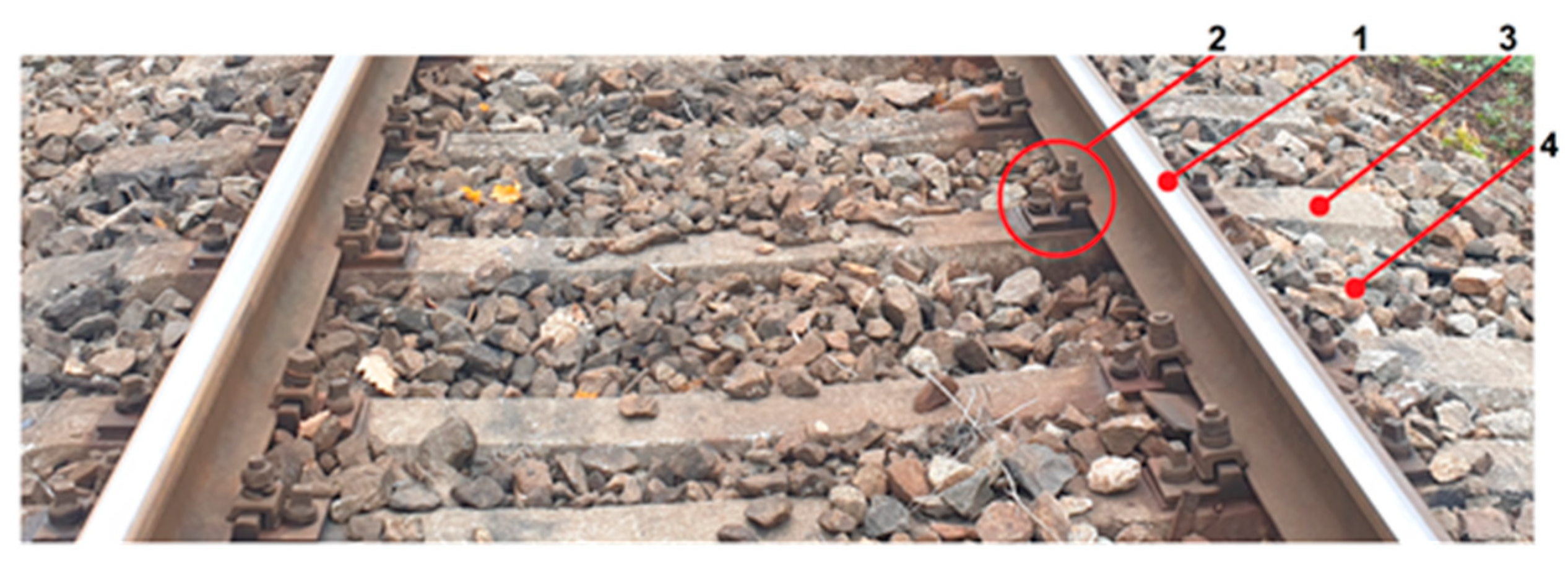
:1. Introduction
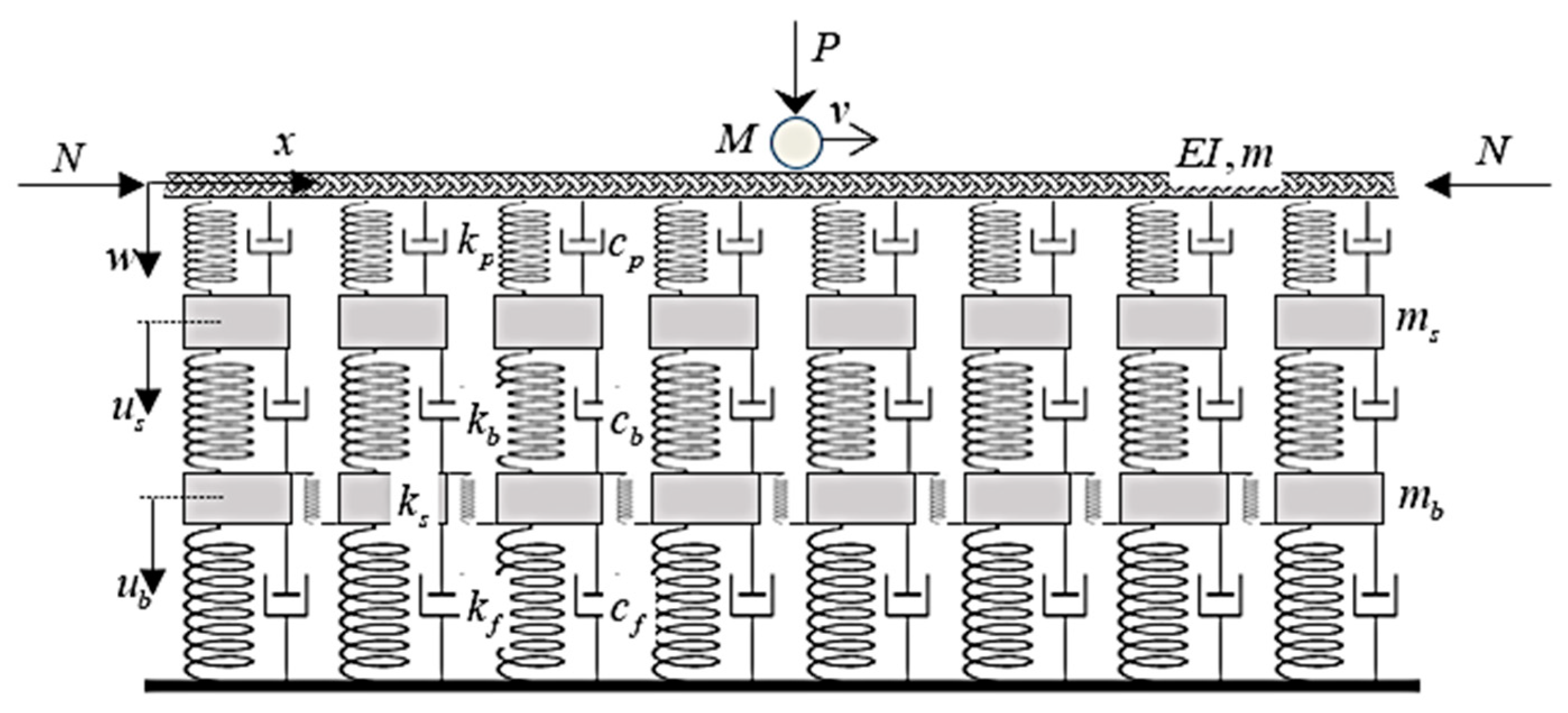
2. Mechanical Model and Governing Equations
- (i)
- The beam is straight and prismatic, and it is made of isotropic homogeneous material.
- (ii)
- The beam can withstand an axial force, in accordance with Figure 2.
- (iii)
- The beam obeys the linear elastic Euler–Bernoulli theory.
- (iv)
- Vertical displacements are measured from the equilibrium position corresponding to the deflection induced by the weight of the model components.
- (v)
- The initial conditions are homogeneous; nevertheless, this has no effect on the critical velocity.
- (vi)
- The velocity of the moving mass determines its horizontal position.
- (vii)
- No friction acts at the contact point.
- (viii)
- Loads and vertical displacements are assumed to be positive when acting downward.
- (ix)
- As is usual in several applications, the acting force may or may not represent the moving mass weight.
3. Semi-Analytical Approach
3.1. Solution of the Governing Equations
3.2. Critical Velocity of a Moving Mass
3.3. Critical Velocity of a Moving Force
3.4. Long Finite Beam—Eigenmode Expansion
4. Green’s Function Method
4.1. Stability Issue
4.2. Time-Domain Response
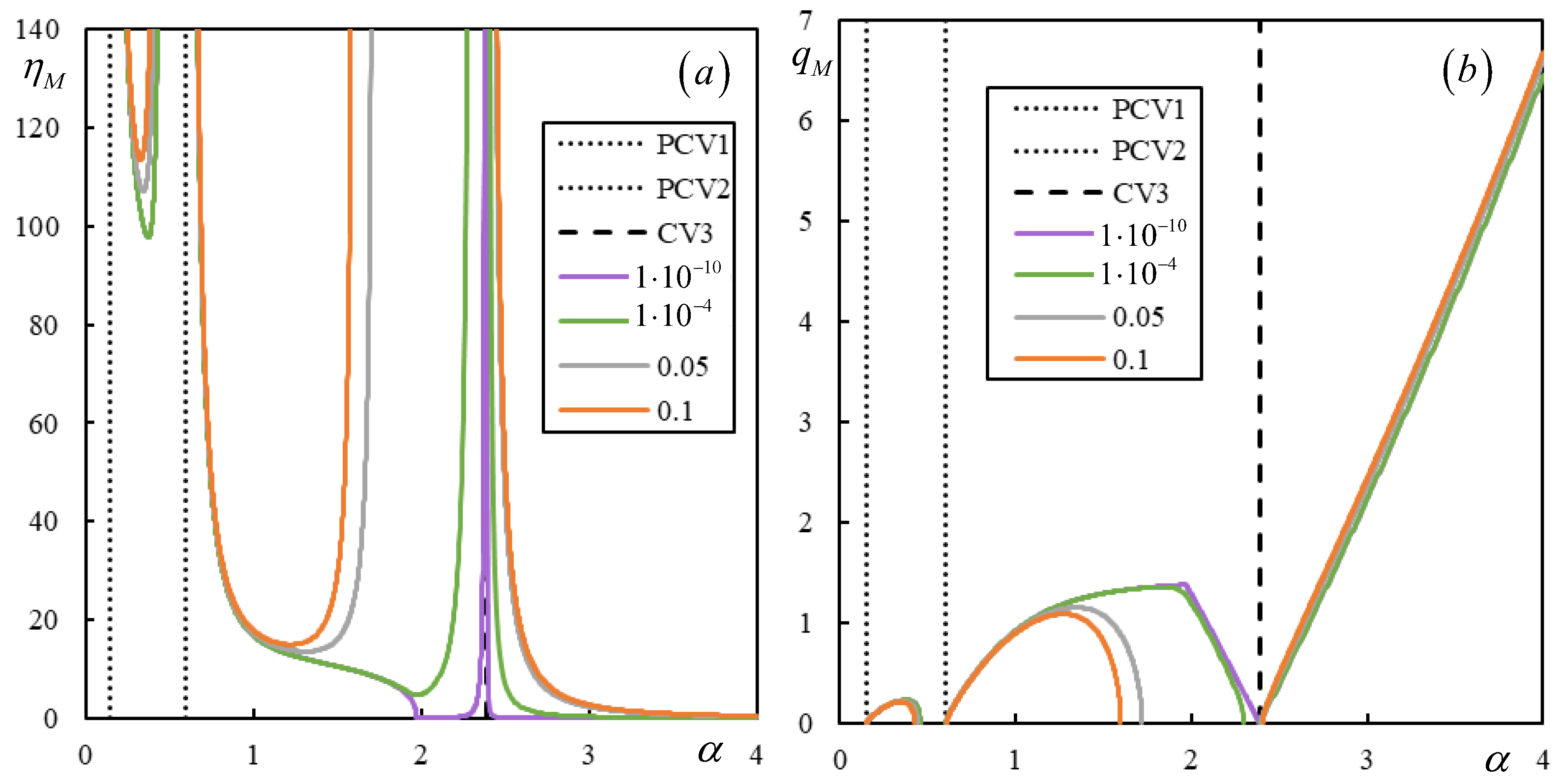
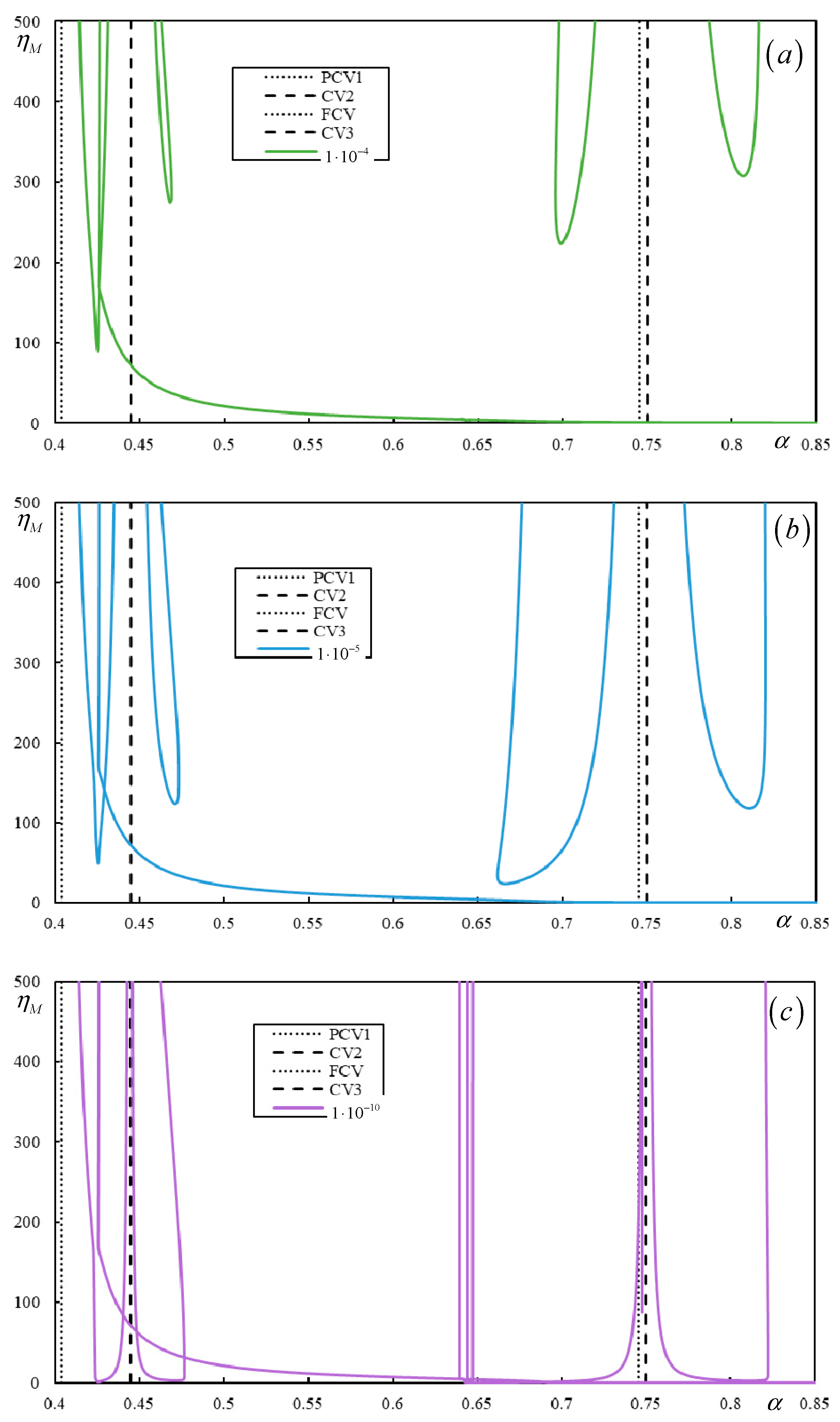
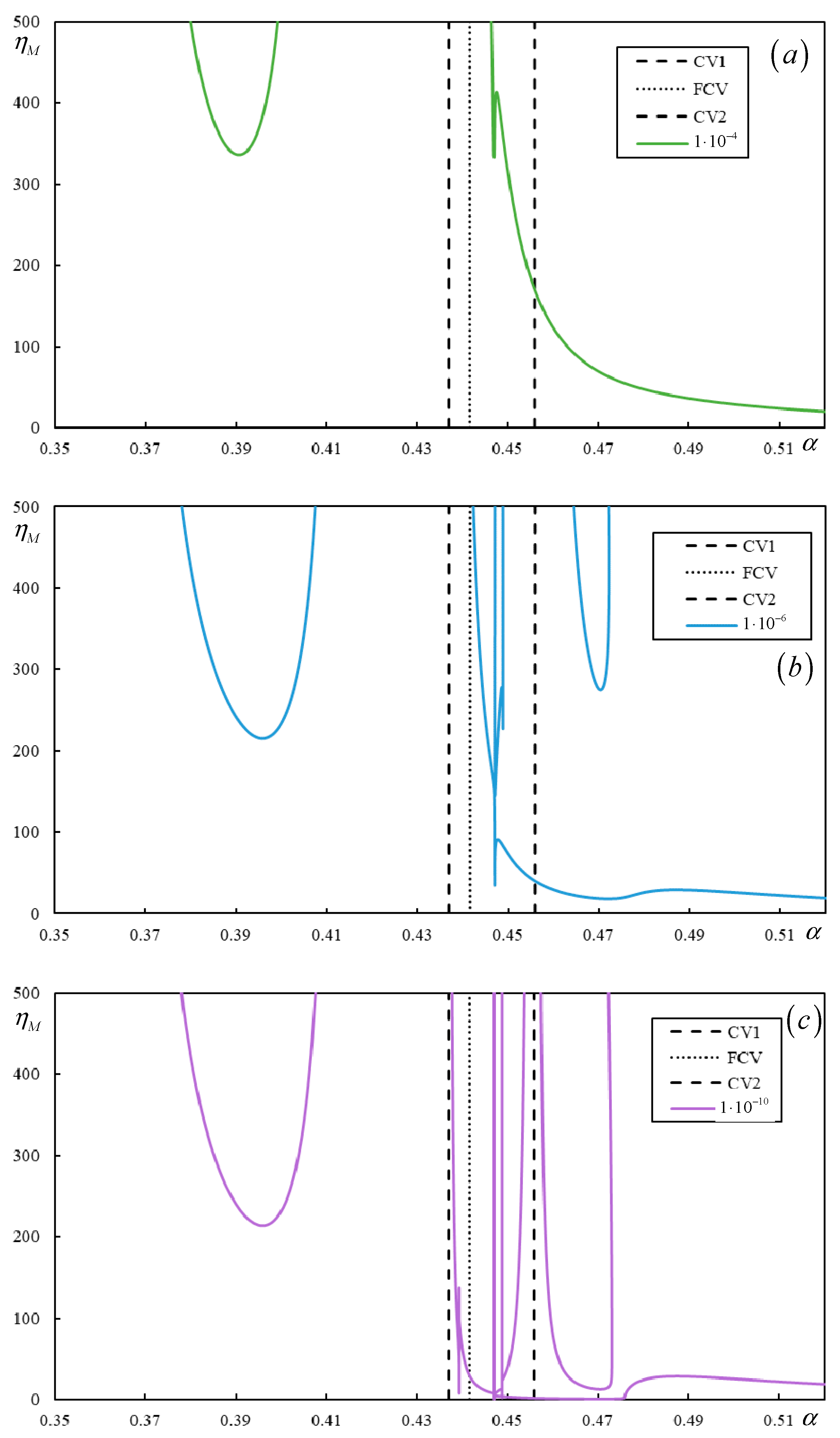
5. Numerical Application
5.1. Allowable Intervals of Dimensionless Parameters
5.2. Test Case from [73]
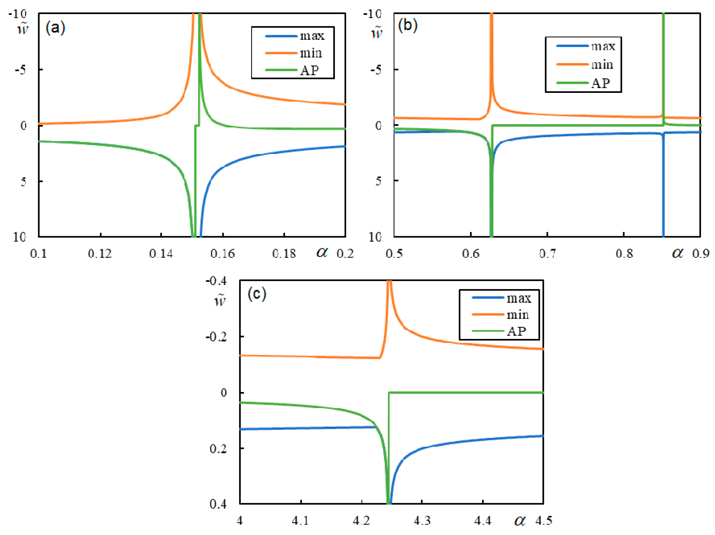
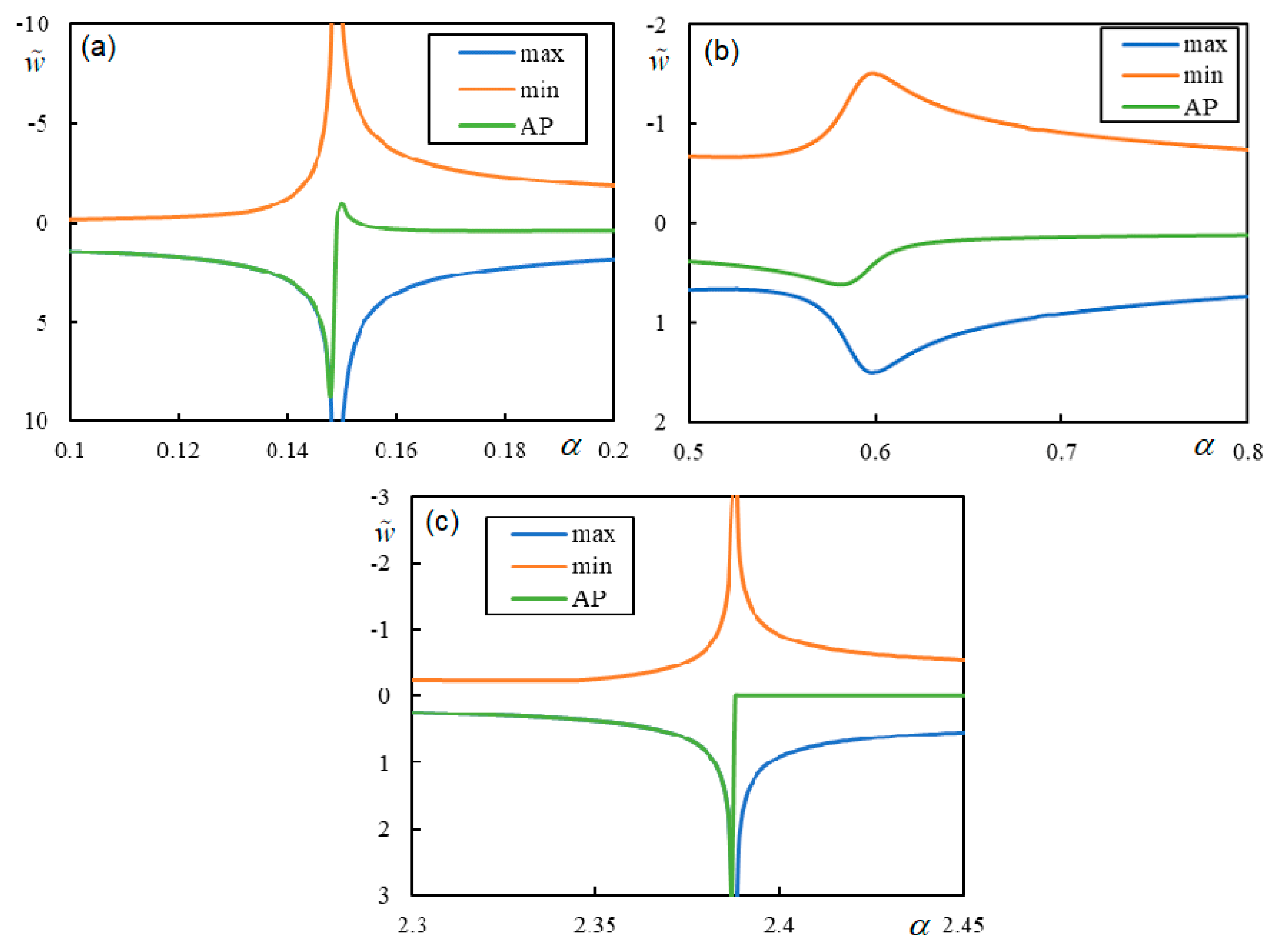
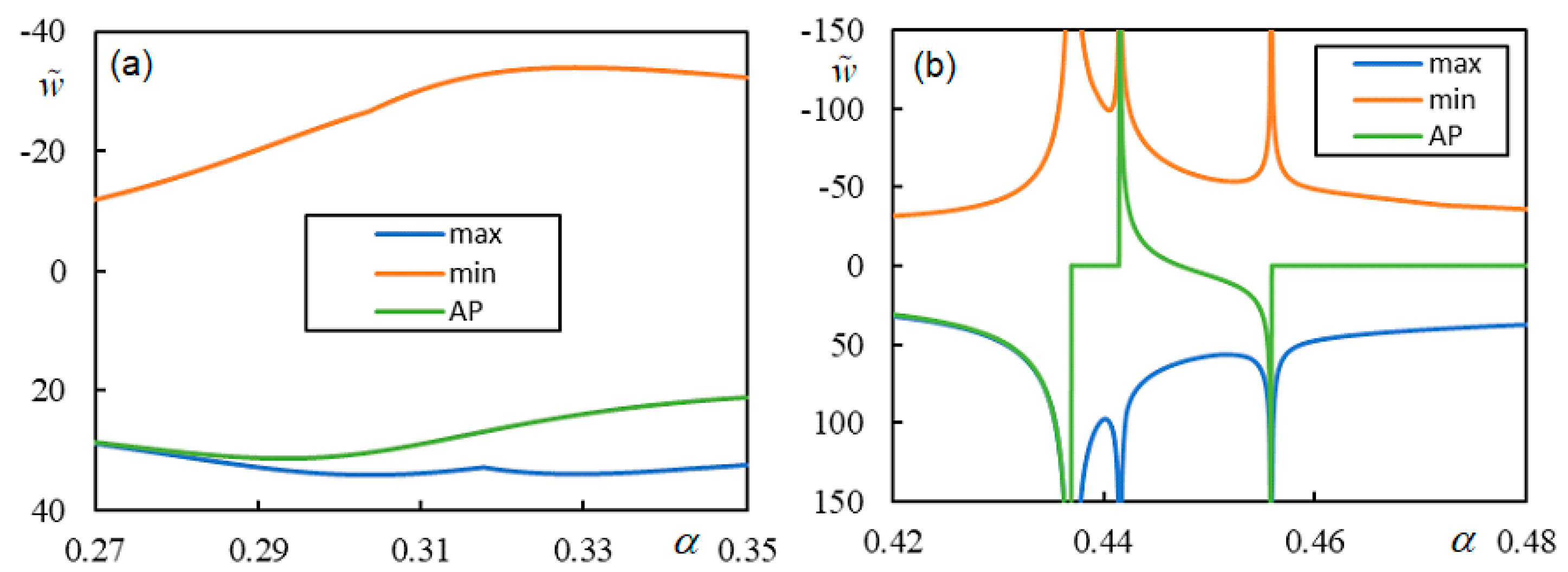
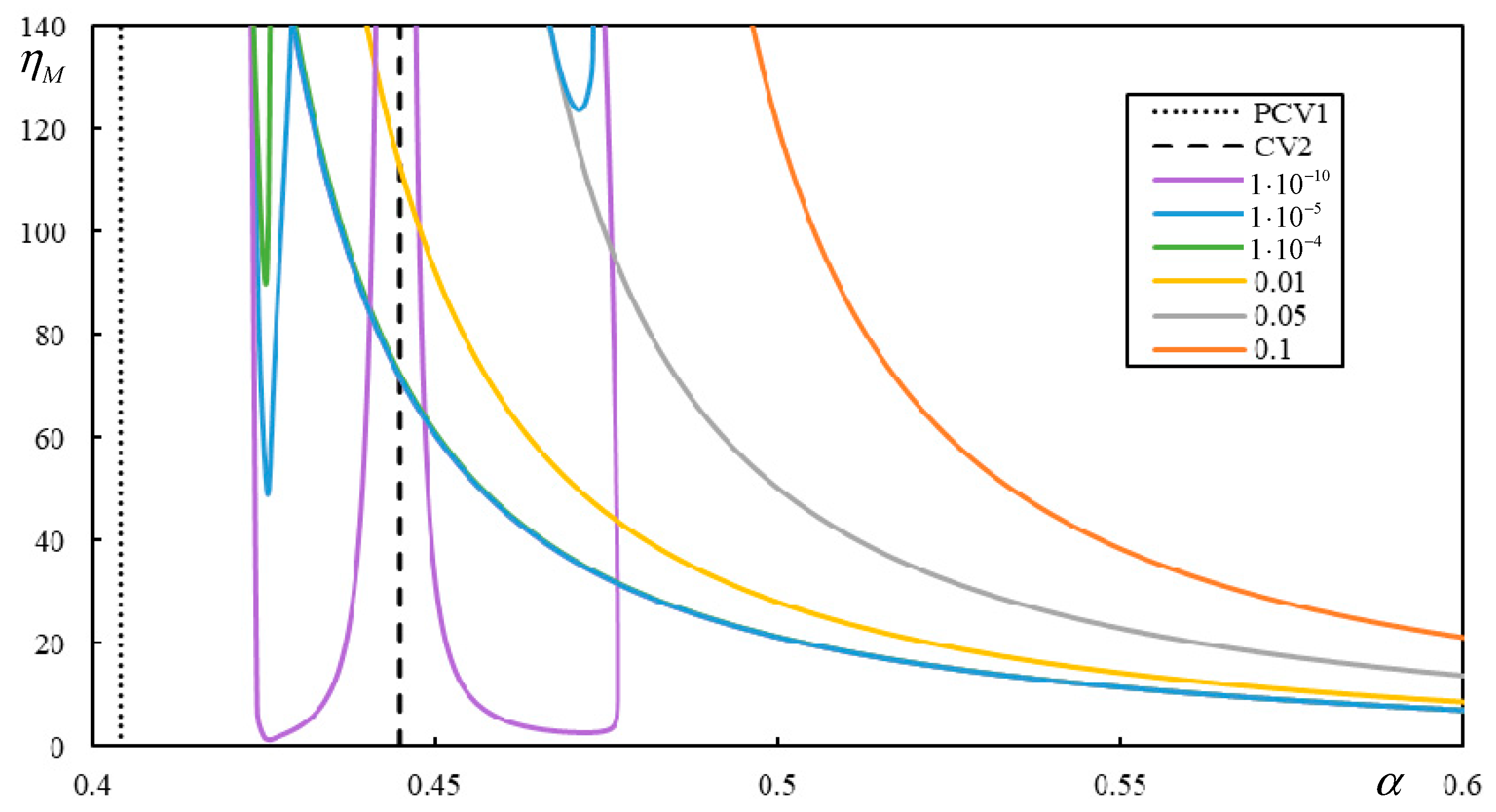
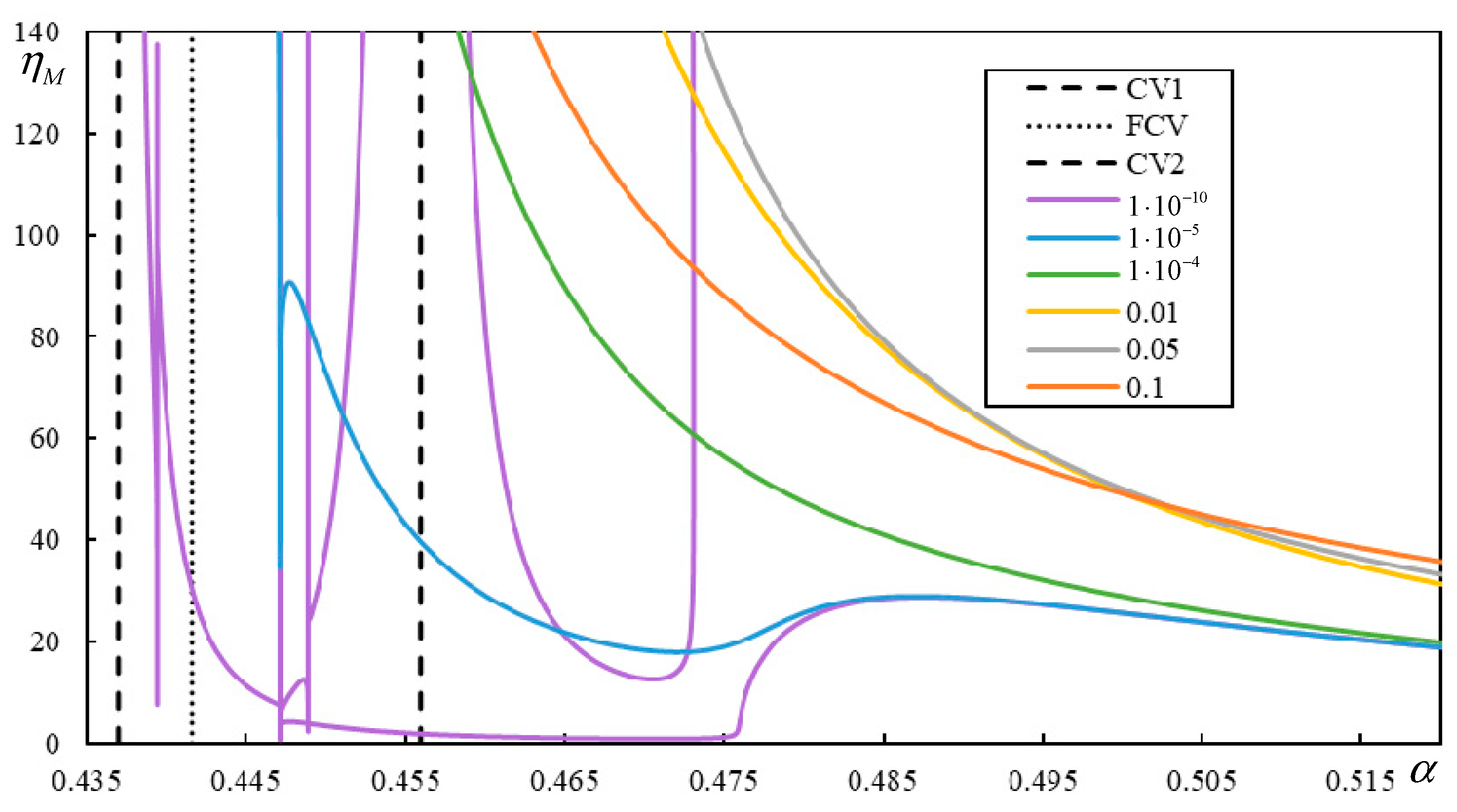
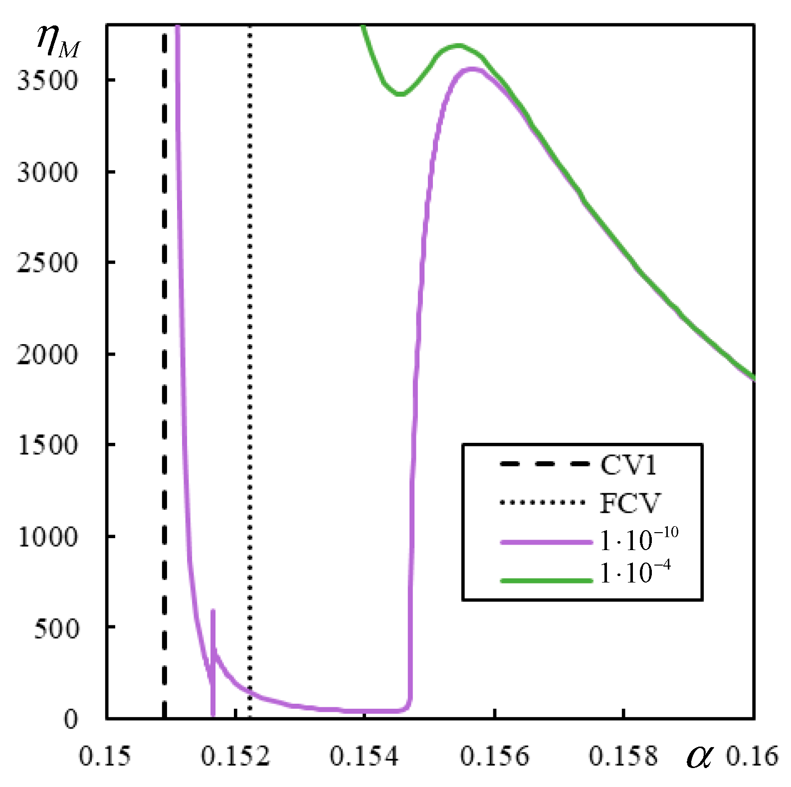
5.3. Other Test Cases
- (i)
- There is at most one instability branch in each of the three regions delimited by CVs and PCVs;
- (ii)
- No branch intersects CV or PCV;
- (iii)
- Branches that correspond to lower damping are below the ones with higher damping, and they do not cross;
- (iv)
- In the first two regions, the branches asymptotically tend to infinite ηM, and in the last region, they asymptotically tend to infinite ηM from the left and zero ηM from the right.
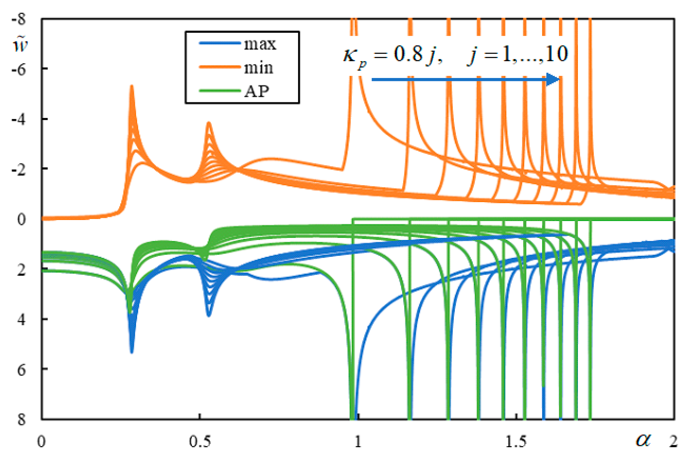
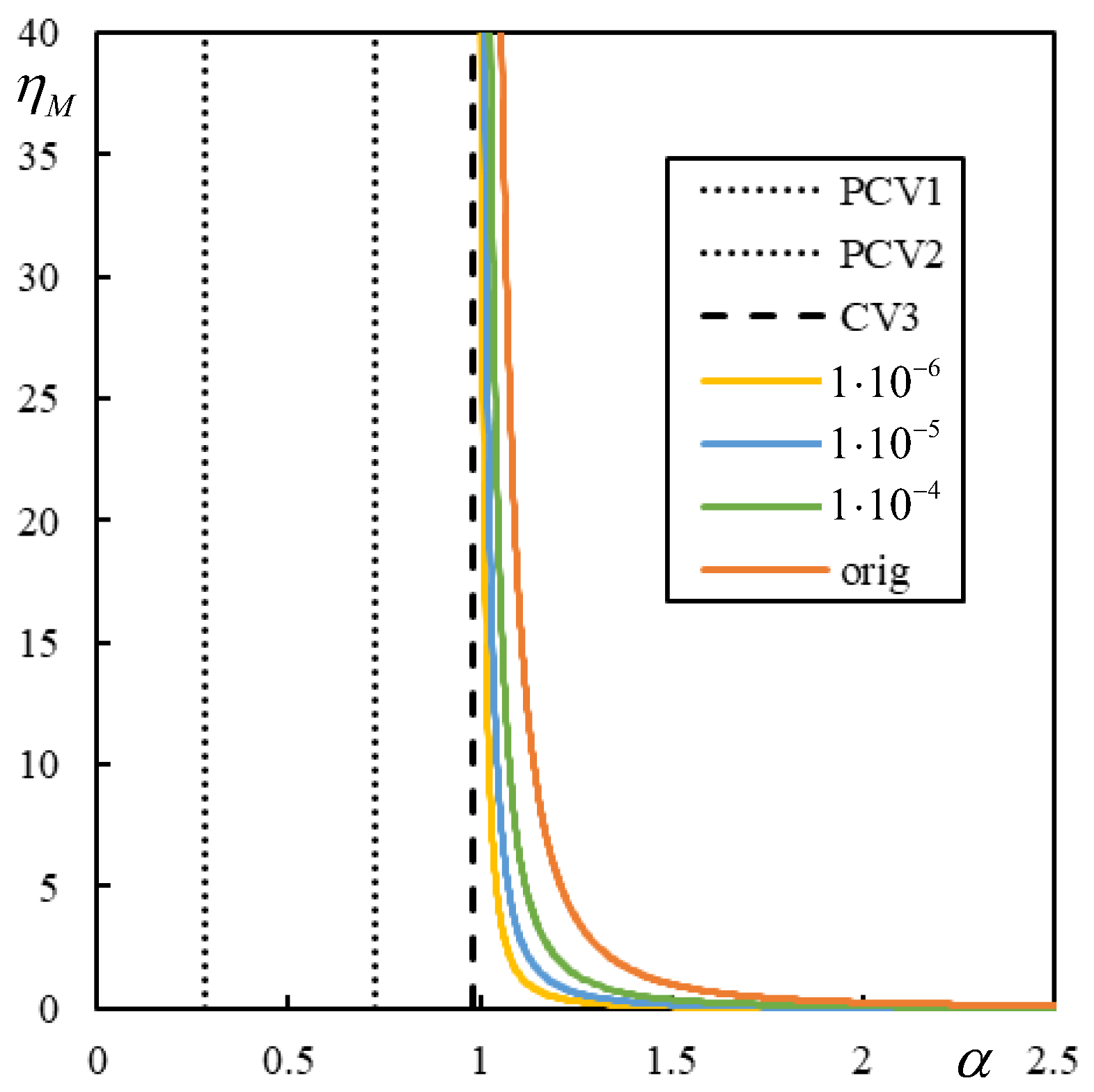
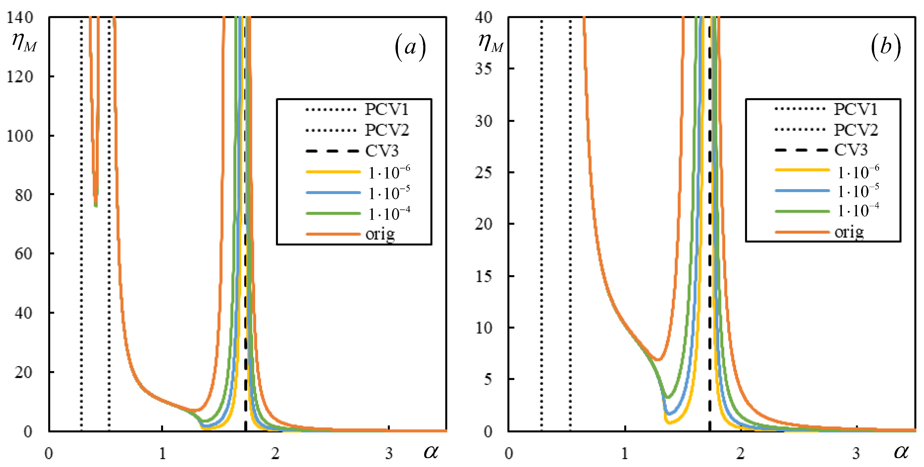
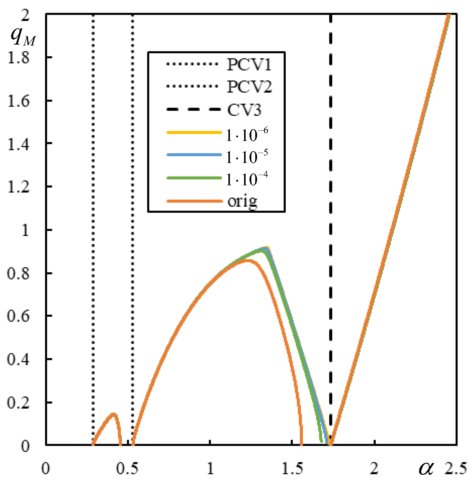
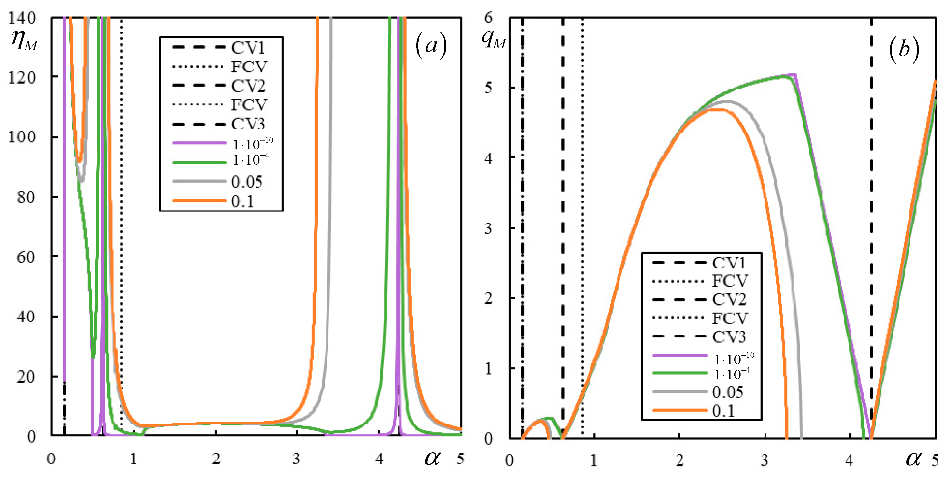
5.4. Influence of the Damping of the Materials in the Foundation
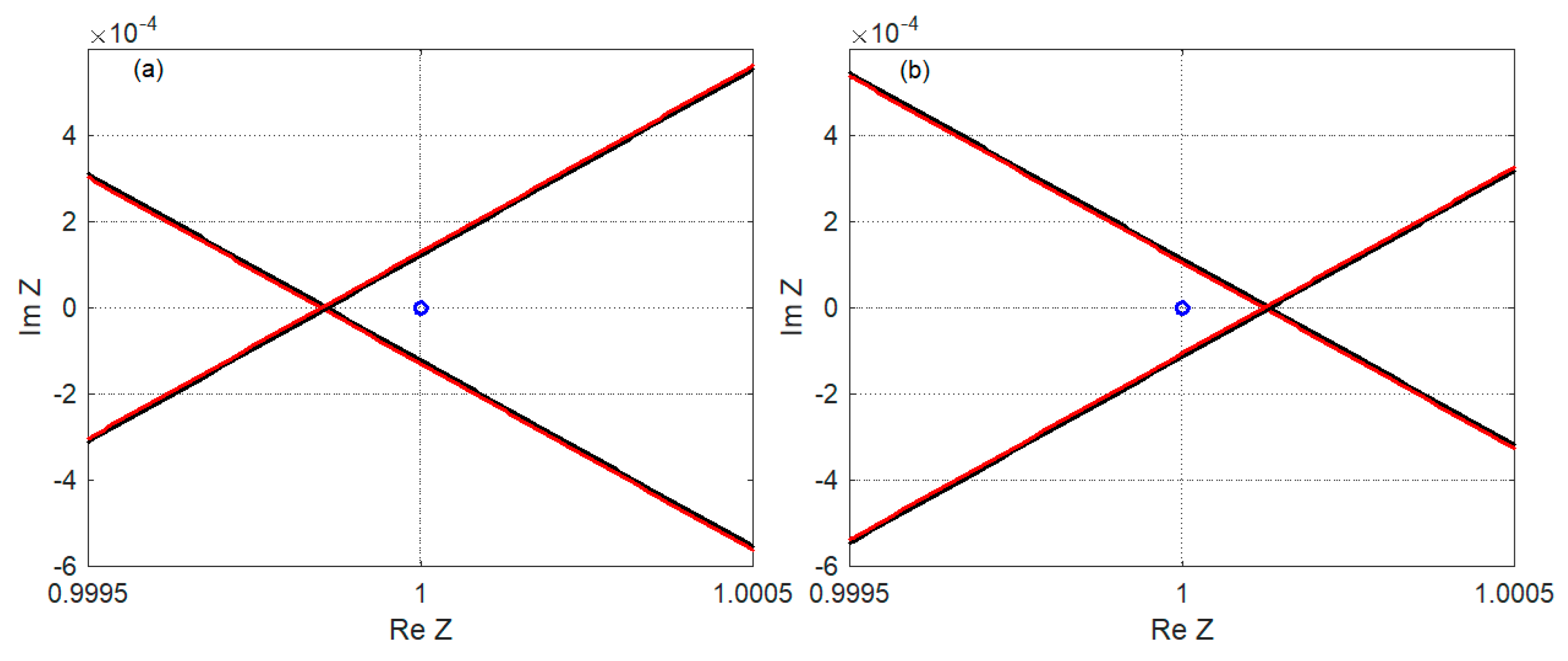
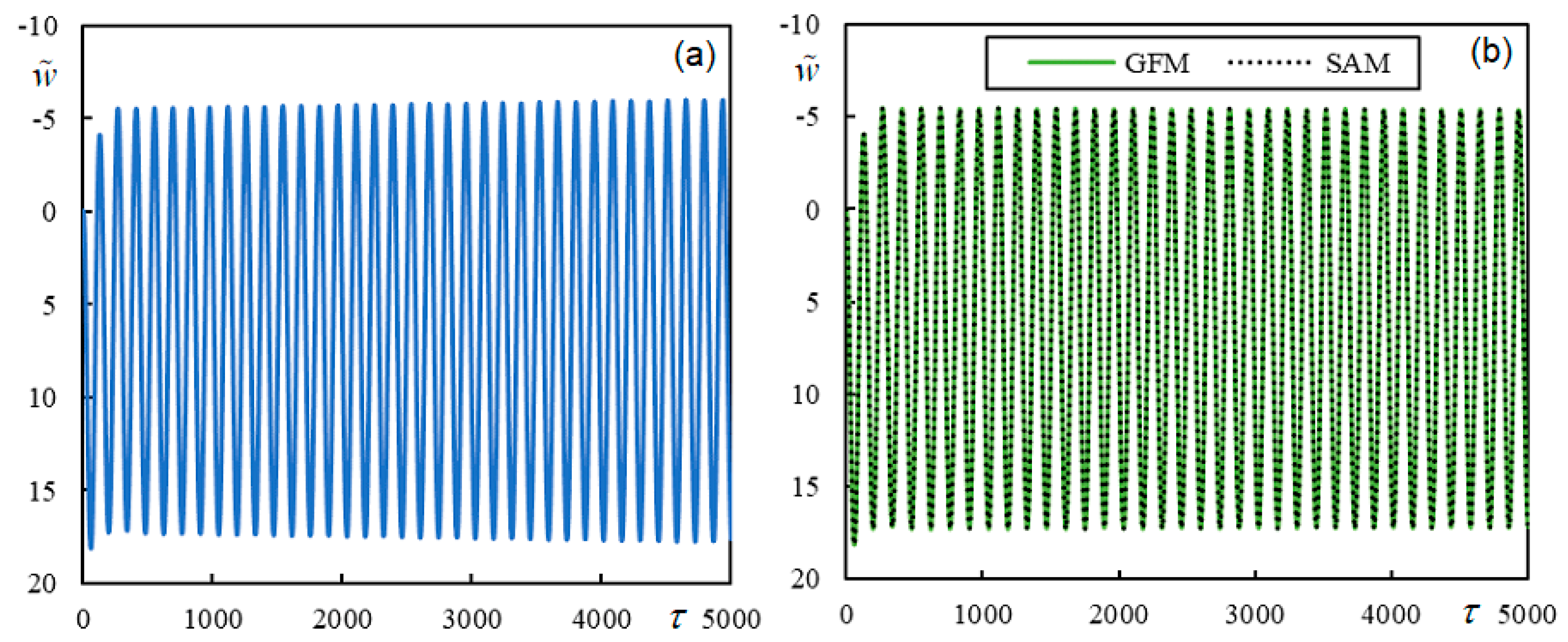
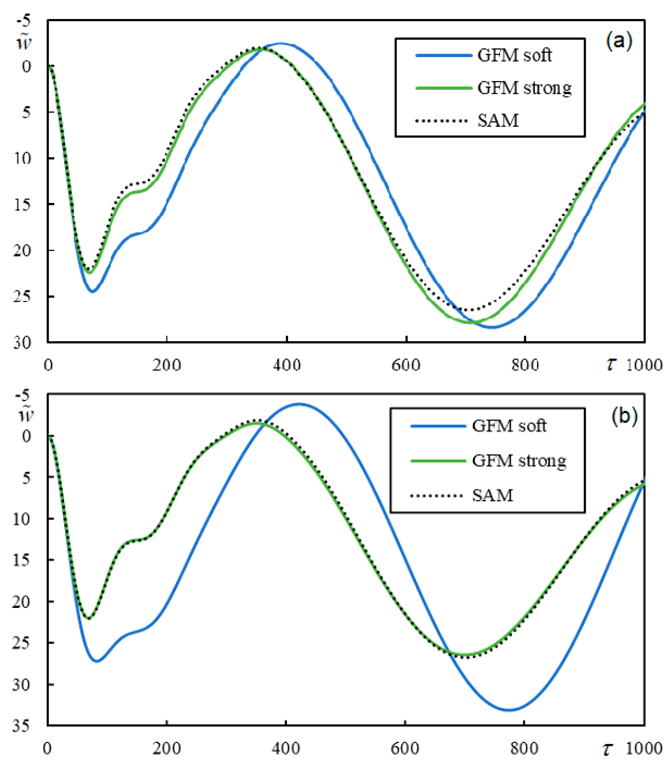
5.5. Comparison between the Results Obtained Using the Semi-Analytical Method and Green’s Function Method
6. Conclusions
Author Contributions
Funding
Institutional Review Board Statement
Informed Consent Statement
Data Availability Statement
Conflicts of Interest
Appendix A
References
- Fortin, J.P. La déformée dynamique de la voie ferrée (Dynamic flexibility of railway track). Rev. Général Chemins. Fer. 1982, 42, 93–102. [Google Scholar]
- Madshus, C.; Kaynia, A.M. High-speed railway lines on soft ground: Dynamic behaviour at critical train speed. J. Sound Vib. 2000, 231, 689–701. [Google Scholar] [CrossRef]
- Szolc, T. On discrete-continuous modelling of the railway bogie and the track for the medium frequency dynamic analysis. Eng. Trans. 2000, 48, 153–198. [Google Scholar]
- Di Gialleonardo, E.; Braghi, F.; Bruni, S. The influence of track modelling options on the simulation of rail vehicle dynamics. J. Sound Vib. 2012, 331, 4246–4258. [Google Scholar] [CrossRef]
- Dumitriu, M. Fault detection of damper in railway vehicle suspension based on the cross-correlation analysis of bogie accelerations. Mech. Ind. 2019, 20, 102. [Google Scholar] [CrossRef]
- Dumitriu, M. A new passive approach to reducing the carbody vertical bending vibration of railway vehicles. Veh. Syst. Dyn. 2017, 55, 1787–1806. [Google Scholar] [CrossRef]
- Zhou, J.; Goodall, R.; Ren, L.; Zhang, H. Influences of car body vertical flexibility on ride quality of passenger railway vehicles. Proc. Inst. Mech. Eng. Part F J. Rail Rapid Transit 2009, 223, 461–471. [Google Scholar] [CrossRef]
- Mazilu, T.; Răcănel, I.R.; Gheți, M.A. Vertical interaction between a driving wheelset and track in the presence of the rolling surfaces harmonic irregularities. Rom. J. Transp. Infrastruct. 2020, 9, 38–52. [Google Scholar] [CrossRef]
- Kerr, A. Elastic and viscoelastic foundation models. J. Appl. Mech. 1994, 31, 491–498. [Google Scholar] [CrossRef]
- Dimitrovová, Z. New semi-analytical solution for a uniformly moving mass on a beam on a two-parameter visco-elastic foundation. Int. J. Mech. Sci. 2017, 127, 142–162. [Google Scholar] [CrossRef]
- Dimitrovová, Z. Semi-analytical analysis of vibrations induced by a mass traversing a beam supported by a finite depth foundation with simplified shear resistance. Meccanica 2020, 55, 2353–2389. [Google Scholar] [CrossRef]
- Mazilu, T. Interaction between moving tandem wheels and an infinite rail with periodic supports—Green’s matrices of the track method in stationary reference frame. J. Sound Vib. 2017, 401, 233–254. [Google Scholar] [CrossRef]
- Nielsen, J.C.O. High-frequency vertical wheel–rail contact forces—Validation of a prediction model by field testing. Wear 2008, 265, 1465–1471. [Google Scholar] [CrossRef]
- Grassie, S.L.; Gregory, R.W.; Harrison, D.; Johnson, K.L. The dynamic response of railway track to high frequency vertical excitation. J. Mech. Eng. Sci. 1982, 24, 77–90. [Google Scholar] [CrossRef]
- Koroma, S.G.; Thompson, D.J.; Hussein, M.F.M.; Ntotsios, E. A mixed space-time and wavenumber-frequency domain procedure for modelling ground vibration from surface railway tracks. J. Sound Vib. 2017, 400, 508–532. [Google Scholar] [CrossRef]
- Cheng, G.; He, Y.; Han, J.; Sheng, X.; Thompson, D. An investigation into the effect of modelling assumptions on sound power radiated from a high-speed train wheelset. J. Sound Vib. 2021, 495, 115910. [Google Scholar] [CrossRef]
- Punetha, P.; Nimbalkar, S. Numerical investigation on dynamic behaviour of critical zones in railway tracks under moving train loads. Transp. Geotech. 2023, 41, 101009. [Google Scholar] [CrossRef]
- Mortensen, J.; Faurholt, J.F.; Hovad, E.; Walther, J.H. Discrete element modelling of track ballast capturing the true shape of ballast stones. Powder Technol. 2021, 386, 144–153. [Google Scholar] [CrossRef]
- Guo, Y.; Zhao, C.; Markine, V.; Jing, G.; Zhai, W. Calibration for discrete element modelling of railway ballast: A review. Transp. Geotech. 2020, 23, 100341. [Google Scholar] [CrossRef]
- Zhang, X.; Thompson, D.J.; Squicciarini, G. Sound radiation from railway sleepers. J. Sound Vib. 2016, 369, 178–194. [Google Scholar] [CrossRef]
- Zhang, X.; Thompson, D.; Quaranta, E.; Squicciarini, G. An engineering model for the prediction of the sound radiation from a railway track. J. Sound Vib. 2019, 461, 114921. [Google Scholar] [CrossRef]
- Koh, C.G.; Ong, J.S.Y.; Chua, D.K.H.; Feng, J. Moving element method for train-track dynamics. Int. J. Numer. Methods Eng. 2003, 56, 1549–1567. [Google Scholar] [CrossRef]
- Ang, K.K.; Dai, J. Response analysis of high-speed rail system accounting for abrupt change of foundation stiffness. J. Sound Vib. 2013, 332, 2954–2970. [Google Scholar] [CrossRef]
- Xu, Y.; Zhu, W.; Fan, W.; Yang, C.; Zhang, W. A new three-dimensional moving Timoshenko beam element for moving load problem analysis. J. Vib. Acoust. Trans. ASME 2020, 142, 031001. [Google Scholar] [CrossRef]
- Elhuni, H.; Basu, D. Novel Nonlinear Dynamic Beam-Foundation Interaction Model. ASCE J. Eng. Mech. 2021, 147, 04021012. [Google Scholar] [CrossRef]
- Metrikine, A.V.; Popp, K. Instability of vibrations of an oscillator moving along a beam on an elastic half-space. Eur. J. Mech. A Solids 1999, 18, 331–349. [Google Scholar] [CrossRef]
- Kerr, A.D. The continuously supported rail subjected to an axial force and a moving load. Int. J. Mech. Sci. 1971, 14, 71–78. [Google Scholar] [CrossRef]
- Metrikine, A.V.; Dieterman, H.A. Instability of vibrations of a mass moving uniformly along an axially compressed beam on a viscoelastic foundation. J. Sound Vib. 1997, 201, 567–576. [Google Scholar] [CrossRef]
- Metrikine, A.V. Unstable lateral oscillations of an object moving uniformly along an elastic guide as a result of an anomalous Doppler effect. Acoust. Phys. 1994, 40, 85–89. [Google Scholar]
- Metrikine, A.V.; Verichev, S.N. Instability of vibrations of a moving two-mass oscillator on a flexibly supported Timoshenko beam. Arch. Appl. Mech. 2001, 71, 613–624. [Google Scholar] [CrossRef]
- Duffy, D.G. The response of an infinite railroad track to a moving, vibrating mass. J. Appl. Mech. 1990, 57, 66–73. [Google Scholar] [CrossRef]
- Mazilu, T.; Dumitriu, M.; Tudorache, C. On the dynamics of interaction between a moving mass and an infinite one-dimensional elastic structure at the stability limit. J. Sound Vib. 2011, 330, 3729–3743. [Google Scholar] [CrossRef]
- Stojanović, V.; Kozić, P.; Petković, M.D. Dynamic instability and critical velocity of a mass moving uniformly along a stabilized infinity beam. Int. J. Solids Struct. 2017, 108, 164–174. [Google Scholar] [CrossRef]
- Dimitrovová, Z. Dynamic interaction and instability of two moving proximate masses on a beam on a Pasternak viscoelastic foundation. Appl. Math. Modell. 2021, 100, 192–217. [Google Scholar] [CrossRef]
- Dimitrovová, Z. Two-layer model of the railway track: Analysis of the critical velocity and instability of two moving proximate masses. Int. J. Mech. Sci. 2022, 217, 107042. [Google Scholar] [CrossRef]
- Metrikine, A.V.; Verichev, S.N.; Blaauwendraad, J. Stability of a two-mass oscillator moving on a beam supported by a visco-elastic half-space. Int. J. Solids Struct. 2005, 42, 1187–1207. [Google Scholar] [CrossRef]
- Stojanović, V.; Petković, M.D.; Deng, J. Stability and vibrations of an overcritical speed moving multiple discrete oscillators along an infinite continuous structure. Eur. J. Mech. A/Solids 2019, 75, 367–380. [Google Scholar] [CrossRef]
- Dimitrovová, Z. Semi-analytical solution for a problem of a uniformly moving oscillator on an infinite beam on a two-parameter visco-elastic foundation. J. Sound Vib. 2019, 438, 257–290. [Google Scholar] [CrossRef]
- Mazilu, T. Instability of a train of oscillators moving along a beam on a viscoelastic foundation. J. Sound Vib. 2013, 332, 4597–4619. [Google Scholar] [CrossRef]
- Yang, B.; Gao, H.; Liu, S. Vibrations of a Multi-Span Beam Structure Carrying Many Moving Oscillators. Int. J. Struct. Stab. Dyn. 2018, 18, 1850125. [Google Scholar] [CrossRef]
- Roy, S.; Chakraborty, G.; DasGupta, A. Coupled dynamics of a viscoelastically supported infinite string and a number of discrete mechanical systems moving with uniform speed. J. Sound Vib. 2018, 415, 184–209. [Google Scholar] [CrossRef]
- Mazilu, T.; Dumitriu, M.; Tudorache, C. Instability of an oscillator moving along a Timoshenko beam on viscoelastic foundation. Nonlinear Dyn. 2012, 67, 1273–1293. [Google Scholar] [CrossRef]
- Verichev, S.N.; Metrikine, A.V. Instability of a bogie moving on a flexibly supported Timoshenko beam. J. Sound Vib. 2002, 253, 653–668. [Google Scholar] [CrossRef]
- Stojanović, V.; Deng, J.; Petković, M.; Milić, D. Non-stability of a bogie moving along a specific infinite complex flexibly beam-layer structure. Eng. Struct. 2023, 295, 116788. [Google Scholar] [CrossRef]
- Nelson, H.D.; Conover, R.A. Dynamic stability of a beam carrying moving masses. J. Appl. Mech. Trans. ASME 1971, 38, 1003–1006. [Google Scholar] [CrossRef]
- Benedetti, G.A. Dynamic stability of a beam loaded by a sequence of moving mass particles. J. Appl. Mech. Trans. ASME 1974, 41, 1069–1071. [Google Scholar] [CrossRef]
- Nassef, A.S.E.; Nassar, M.M.; EL-Refaee, M.M. Dynamic response of Timoshenko beam resting on nonlinear Pasternak foundation carrying sprung masses. Iran. J. Sci. Technol. Trans. Mech. Eng. 2019, 43, 419–426. [Google Scholar] [CrossRef]
- Stojanović, V.; Petković, M.; Deng, J. Instability of vehicle systems moving along an infinite beam on a viscoelastic foundation. Eur. J. Mech. A. Solids. 2018, 69, 238–254. [Google Scholar] [CrossRef]
- Stojanović, V.; Deng, J.; Milić, D.; Petković, M.D. Dynamics of moving coupled objects with stabilizers and unconventional couplings. J. Sound Vib. 2024, 570, 118020. [Google Scholar] [CrossRef]
- Mazilu, T. Stability of vibration of a moving mass on an elastically supported beam. In Proceedings of the 2nd WSEAS International Conference on Engineering Mechanics, Structures and Engineering Geology (EMESEG ‘09), Rodos, Greece, 22–24 July 2009. [Google Scholar]
- Dimitrovová, Z. Instability of vibrations of mass(es) moving uniformly on a two-layer track model: Parameters leading to irregular cases and associated implications for railway design. Appl. Sci. 2023, 13, 12356. [Google Scholar] [CrossRef]
- Dimitrovová, Z. On the critical velocity of moving force and instability of moving mass in layered railway track models by semianalytical approaches. Vibration 2023, 6, 113–146. [Google Scholar] [CrossRef]
- Yang, C.J.; Xu, Y.; Zhu, W.D.; Fan, W.; Zhang, W.H.; Mei, G.M. A three-dimensional modal theory-based Timoshenko finite length beam model for train-track dynamic analysis. J. Sound Vib. 2020, 479, 115363. [Google Scholar] [CrossRef]
- Abea, K.; Chidaa, Y.; Quinay, P.E.B.; Koroa, K. Dynamic instability of a wheel moving on a discretely supported infinite rail. J. Sound Vib. 2014, 333, 3413–3427. [Google Scholar] [CrossRef]
- Kiani, K.; Nikkhoo, A. On the limitations of linear beams for the problems of moving mass-beam interaction using a meshfree method. Acta Mech. Sin. 2011, 28, 164–179. [Google Scholar] [CrossRef]
- Kiani, K.; Nikkhoo, A.; Mehri, B. Prediction capabilities of classical and shear deformable beam models excited by a moving mass. J. Sound Vib. 2009, 320, 632–648. [Google Scholar] [CrossRef]
- Kiani, K.; Nikkhoo, A.; Mehri, B. Assessing dynamic response of multispan viscoelastic thin beams under a moving mass via generalized moving least square method. Acta Mech. Sin. 2010, 26, 721–733. [Google Scholar] [CrossRef]
- Jahangiri, A.; Attari, N.K.A.; Nikkhoo, A.; Waezi, Z. Nonlinear dynamic response of an Euler–Bernoulli beam under a moving mass–spring with large oscillations. Arch. Appl. Mech. 2020, 90, 1135–1156. [Google Scholar] [CrossRef]
- Dimitrovová, Z. Complete semi-analytical solution for a uniformly moving mass on a beam on a two-parameter visco-elastic foundation with non-homogeneous initial conditions. Int. J. Mech. Sci. 2018, 144, 283–311. [Google Scholar] [CrossRef]
- Tran, M.T.; Ang, K.K.; Luong, V.H. Vertical dynamic response of non-uniform motion of high-speed rails. J. Sound Vib. 2014, 333, 5427–5442. [Google Scholar] [CrossRef]
- Fărăgău, A.B.; Metrikine, A.V.; van Dalen, K.N. Transition radiation in a piecewise-linear and infinite one-dimensional structure–a Laplace transform method. Nonlinear Dyn. 2019, 98, 2435–2461. [Google Scholar] [CrossRef]
- Fărăgău, A.B.; Keijdener, C.; de Oliveira Barbosa, J.M.; Metrikine, A.V.; van Dalen, K.N. Transition radiation in a nonlinear and infinite one-dimensional structure: A comparison of solution methods. Nonlinear Dyn. 2021, 103, 1365–1391. [Google Scholar] [CrossRef]
- Dai, J.; Lim, J.G.Y.; Ang, K.K. Dynamic response analysis of high-speed maglev-guideway system. J. Vib. Eng. Technol. 2023, 11, 2647–2658. [Google Scholar] [CrossRef]
- Song, Y.; Wang, Z.; Liu, Z.; Wang, R. A spatial coupling model to study dynamic performance of pantograph-catenary with vehicle-track excitation. Mech. Syst. Signal Process. 2021, 151, 107336. [Google Scholar] [CrossRef]
- Bruni, S.; Bucca, G.; Carnavale, M.; Collina, A.; Fanccinetti, A. Pantograph–catenary interaction: Recent achievements and future research challenges. Int. J. Rail Transp. 2018, 6, 57–82. [Google Scholar] [CrossRef]
- Frýba, L. Vibration of Solids and Structures under Moving Loads, Research Institute of Transport, Prague (1972), 3rd ed.; Thomas Telford: London, UK, 1999. [Google Scholar]
- Dieterman, H.A.; Metrikine, A.V. Steady state displacements of a beam on an elastic half-space due to uniformly moving constant load. Eur. J. Mech. A/Solids 1997, 16, 295–306. [Google Scholar]
- Ramos, A.; Castanheira-Pinto, A.; Colaço, A.; Fernández-Ruiz, J.; Costa, P.A. Predicting Critical Speed of Railway Tracks Using Artificial Intelligence Algorithms. Vibration 2023, 6, 895–916. [Google Scholar] [CrossRef]
- Neimark, Y.I. Dynamic Systems and Controllable Processes; Nauka: Moscow, Russia, 1978. (In Russian) [Google Scholar]
- Mazilu, T. Green’s functions for analysis of dynamic response of wheel/rail to vertical excitation. J. Sound Vib. 2007, 306, 31–58. [Google Scholar] [CrossRef]
- Rodrigues, A.S.F. Viability and Applicability of Simplified Models for the Dynamic Analysis of Ballasted Railway Tracks. Ph.D. Thesis, Faculdade de Ciências e Tecnologia da Universidade Nova de Lisboa, Caparica, Portugal, 2017. [Google Scholar]
- Rodrigues, A.S.F.; Dimitrovová, Z. Applicability of a three-layer model for the dynamic analysis of ballasted railway tracks. Vibration 2021, 4, 151–174. [Google Scholar] [CrossRef]
- Zhai, M.W.; Wang, K.Y.; Lin, J.H. Modelling and experiment of railway ballast vibrations. J. Sound Vib. 2004, 270, 673–683. [Google Scholar] [CrossRef]
- Sañudo, R.; Miranda, M.; Alonso, B.; Markine, V. Sleepers spacing analysis in railway track infrastructure. Infrastructures 2022, 7, 83. [Google Scholar] [CrossRef]
- Ortega, R.S.; Pombo, J.; Ricci, S.; Miranda, M. The importance of sleepers spacing in railways. Constr. Build. Mater. 2021, 300, 124326. [Google Scholar] [CrossRef]
- Van Dalen, K.N. Ground Vibration Induced by a High-Speed Train Running over Inhomogeneous Subsoil, Transition Radiation in Two-Dimensional Inhomogeneous Elastic Systems. Master’s Thesis, Department of Structural Engineering, TUDelft, Delft, The Netherlands, 2006. [Google Scholar]
- Chen, Y.-H.; Huang, Y.-H.; Shih, C.-T. Response of an Infinite Timoshenko Beam on a Viscoelastic Foundation to a Harmonic Moving Load. J. Sound Vib. 2001, 241, 809–824. [Google Scholar] [CrossRef]
- Náprstek, J.; Fischer, C. Interaction of a beam and supporting continuum under moving periodic load. In Proceedings of the 10th International Conference on Computational Structures Technology, Valencia, Spain, 14–17 September 2010; Topping, B.H.V., Adam, J.M., Bru, F.J.P.R., Romcro, M.L., Eds.; Civil-Comp Press: Valencia, Spain, 2010; pp. 20, 38. [Google Scholar]
- Náprstek, J. Cylindrical wave propagation in a visco-elastic continuum generated by a moving load. In Proceedings of the International Symposium on Environmental Vibrations ISEV2007, Taipei, Taiwan, 28–30 November 2007; Yang, Y.B., Yau, Y.D., Eds.; National Taiwan University: Taipei, Taiwan, 2007; pp. 647–654. [Google Scholar]


| Parameter | Approximate Range (with Margins) |
|---|---|
| EI (MNm2) | 4.7 or 6.4 |
| m (kg/m) | 54 or 60 |
| ms (kg/m) | 56–294 |
| mb (kg/m) | 117–2377 |
| kp (MN/m2) | 28–9174 |
| kb (MN/m2) | 42–1304 |
| kf (MN/m2) | 0.22–1000 |
| ks (MN/m2) | 0.5–141 |
| Dimensionless Parameter | Approximate Range (with Margins) |
|---|---|
| μs | 1–6 |
| μb | 2–45 |
| κp | 0.03–42,000 |
| κb | 0.04–6000 |
| ηs | 0–70 |
| Case | μs | μb | κp | κb | ηs | Resonances | Type |
|---|---|---|---|---|---|---|---|
| 1 | 6 | 35 | 300 | 7 | 0 | 5 (0.151-CV1; 0.152-FCV; 0.627-CV2; 0.851-FCV; 4.244-CV3) | regular |
| 2 | 6 | 35 | 30 | 7 | 0 | 1 (0.149-PCV1 (nd); 0.599-PCV2; 2.388-CV3)) | regular |
| 3 | 6 | 5 | 0.03 | 3 | 0 | 3 (0.404-PCV1 (d); 0.445-CV2; 0.745-FCV; 0.750-CV3) | irregular |
| 4 | 3 | 10 | 0.03 | 0.1 | 0 | 3 (0.293-PCV1 (nd); 0.437-CV2; 0.442-FCV; 0.456-CV3) | irregular |
Disclaimer/Publisher’s Note: The statements, opinions and data contained in all publications are solely those of the individual author(s) and contributor(s) and not of MDPI and/or the editor(s). MDPI and/or the editor(s) disclaim responsibility for any injury to people or property resulting from any ideas, methods, instructions or products referred to in the content. |
© 2024 by the authors. Licensee MDPI, Basel, Switzerland. This article is an open access article distributed under the terms and conditions of the Creative Commons Attribution (CC BY) license (https://creativecommons.org/licenses/by/4.0/).
Share and Cite
Dimitrovová, Z.; Mazilu, T. Semi-Analytical Approach and Green’s Function Method: A Comparison in the Analysis of the Interaction of a Moving Mass on an Infinite Beam on a Three-Layer Viscoelastic Foundation at the Stability Limit—The Effect of Damping of Foundation Materials. Materials 2024, 17, 279. https://doi.org/10.3390/ma17020279
Dimitrovová Z, Mazilu T. Semi-Analytical Approach and Green’s Function Method: A Comparison in the Analysis of the Interaction of a Moving Mass on an Infinite Beam on a Three-Layer Viscoelastic Foundation at the Stability Limit—The Effect of Damping of Foundation Materials. Materials. 2024; 17(2):279. https://doi.org/10.3390/ma17020279
Chicago/Turabian StyleDimitrovová, Zuzana, and Traian Mazilu. 2024. "Semi-Analytical Approach and Green’s Function Method: A Comparison in the Analysis of the Interaction of a Moving Mass on an Infinite Beam on a Three-Layer Viscoelastic Foundation at the Stability Limit—The Effect of Damping of Foundation Materials" Materials 17, no. 2: 279. https://doi.org/10.3390/ma17020279