
Interaction of Nitrite Ions with Hydrated Portlandite Surfaces: Atomistic Computer Simulation Study

1
International Laboratory for Supercomputer Atomistic Modelling and Multi-Scale Analysis, HSE University, 101000 Moscow, Russia
2
Joint Institute for High Temperatures of the Russian Academy of Sciences, 125412 Moscow, Russia
3
Laboratoire SUBATECH, UMR 6457–Institut Mines Télécom Atlantique, Nantes Université, CNRS/IN2P3, 44307 Nantes, France
*
Author to whom correspondence should be addressed.
Materials 2023, 16(14), 5026; https://doi.org/10.3390/ma16145026
Submission received: 4 June 2023
/
Revised: 12 July 2023
/
Accepted: 14 July 2023
/
Published: 16 July 2023
(This article belongs to the Special Issue Concretes and Cement-Based Composites: Additives/Admixtures, Hydration Process and Durability Research)
Abstract
:The nitrite admixtures in cement and concrete are used as corrosion inhibitors for steel reinforcement and also as anti-freezing agents. The characterization of the protective properties should account for the decrease in the concentration of free NO2− ions in the pores of cement concretes due to their adsorption. Here we applied the classical molecular dynamics computer simulation approach to quantitatively study the molecular scale mechanisms of nitrite adsorption from NaNO2 aqueous solution on a portlandite surface. We used a new parameterization to model the hydrated NO2− ions in combination with the recently upgraded ClayFF force field (ClayFF-MOH) for the structure of portlandite. The new NO2− parameterization makes it possible to reproduce the properties of hydrated NO2− ions in good agreement with experimental data. In addition, the ClayFF-MOH model improves the description of the portlandite structure by explicitly taking into account the bending of Ca-O-H angles in the crystal and on its surface. The simulations showed that despite the formation of a well-structured water layer on the portlandite (001) crystal surface, NO2− ions can be strongly adsorbed. The nitrite adsorption is primarily due to the formation of hydrogen bonds between the structural hydroxyls on the portlandite surface and both the nitrogen and oxygen atoms of the NO2− ions. Due to that, the ions do not form surface adsorption complexes with a single well-defined structure but can assume various local coordinations. However, in all cases, the adsorbed ions did not show significant surface diffusional mobility. Moreover, we demonstrated that the nitrite ions can be adsorbed both near the previously-adsorbed hydrated Na+ ions as surface ion pairs, but also separately from the cations.
Keywords:
portlandite; hydration; nitrite; NO2−; adsorption; hydrogen bonding; molecular dynamics simulation1. Introduction
Cement-based concretes are capillary-porous materials that are often exposed to an aggressive environment (sulfate and chlorine attacks, alkali–aggregate expansion reactions, etc.). This can detrimentally affect the durability of structures made of concrete and reinforced concrete. To increase their durability and sustainability, various chemical additives are used. The application of such chemical additives is one of the effective solutions to green chemistry in concrete production [1]. Calcium and sodium nitrites, Ca(NO2)2 and NaNO2, are important chemical admixtures in the manufacture of concretes based on Portland cement. They inhibit the corrosion of reinforcing steel in reinforced concrete [2,3] and also act as anti-freezing agents [4,5]. It has been found that the nitrite ions, NO2−, bind to the cement surfaces [6]. This process reduces the concentration of free hydrated NO2− in aqueous solutions inside concrete pores, thus reducing the effect of corrosion inhibition in the presence of Cl− ions. Therefore, molecular scale understanding of the hydrated NO2− behavior at the surfaces of cementitious materials is important for reliable prediction of the durability of reinforced concrete structures.
Portlandite, Ca(OH)2, is one of the important mineral phases of hydrated Portland cement, which is involved in the formation of the crystalline framework of hardened cement. The presence of portlandite maintains the high pH of the hardened cement [7], which is another factor protecting the reinforcing steel from corrosion [8]. In this paper, we chose this crystalline phase of hardened cement to quantify, by means of classical atomistic simulations, the structural, dynamic, and energetic aspects of its interactions with nitrite ions. According to experimental data [6], the use of the Ca(NO2)2 admixture can lead to the formation of new Ca(OH)2 crystals on the surface of existing portlandite crystals. This might introduce some undesirable ambiguity into the definition and quantitative analysis of the portlandite-solution interface within our current molecular modeling approaches. Therefore, NaNO2 rather than Ca(NO2)2 was selected for our simulations as a model nitrite admixture.
Methods of atomistic computer simulations make it possible to obtain detailed quantitative information about the adsorption and binding of ions on various surfaces at a fundamental molecular scale. In recent years, they have increasingly become an important and powerful tool in cement research [9,10,11]. The methods of atomistic computational modeling can be roughly subdivided into deterministic and stochastic. The stochastic approach of Monte Carlo (MC) simulations offers a statistical–mechanical description of materials, which is most useful for studying various thermodynamic characteristics, the energetics of adsorption, and other equilibrium properties of the simulated system under given thermodynamic conditions [12,13]. The deterministic approaches of molecular dynamics (MD) are based on the numerical solution of a set of Newtonian equations of motion for a large number of interacting particles (atoms, molecules, ions). In addition to thermodynamic properties, the MD approach also allows the calculation of many important dynamic properties, such as transport coefficients, vibrational spectra, or various relaxation times in the simulated system [14,15]. In the present work, we employed the method of classical MD simulations to model portlandite and its interaction with an interfacial aqueous solution of sodium nitrite. The recently modified version of the ClayFF force field (ClayFF-MOH) [16] with explicit Metal-O-H (MOH) angular bending terms [17] was used to simulate portlandite, while for the hydrated NO2− ions a new parametrization of intermolecular interaction constants was recently developed [18]. Recent molecular simulations of the interfaces between aqueous salt solutions and another significant cement phase of ettringite [19] have already clearly demonstrated the importance of the MOH terms for accurate modeling of the mineral systems containing structural and interfacial hydroxyl groups. In addition to a more accurate reproduction of the properties of hydroxide minerals themselves, the introduction of MOH terms also affects the structural and dynamic properties of aqueous solutions in the near-surface layers of solutions compared to the original version of the ClayFF force field [20,21].
2. Models and Methods
2.1. Structural Models
Portlandite belongs to the group of metal hydroxides; M(OH)2 (M stands for a divalent metal cation), and has a brucite-like layered structure. Portlandite crystals have symmetry and the crystal structure consists of alternating trioctahedral layers along the c-axis that terminate with hydroxyl groups. The layers are formed by distorted edge-sharing CaO6 octahedra, with each hydroxyl ion being linked to three calcium ions [22,23].
An ideal unit cell of portlandite used in this work was built according to the structure determination by neutron diffraction measurements [24] with the lattice parameters of a = 3.59 Å, c = 4.90 Å, γ = 120°. A supercell of 10 × 10 × 8 unit cells along the a, b, and c cell vectors, respectively, was constructed for our simulations. The supercell had dimensions of approximately 35.9 × 35.9 × 39.3 Å3 and contained 4000 atoms.
To simulate the interface of portlandite with NaNO2 aqueous solution, a system consisting of 11 × 10 × 8 portlandite unit cells was cleaved parallel to the (001) plane and cut in the ab plane of the crystal to a rectangular shape. The (001) interface orientation is chosen because it has one of the lowest cleavage-free energies of all possible portlandite crystal faces [25,26,27,28]. Despite its hydrophilicity, the (001) crystal surface is more resistant to dissolution in water compared to other crystal faces of portlandite and brucite [29,30,31].
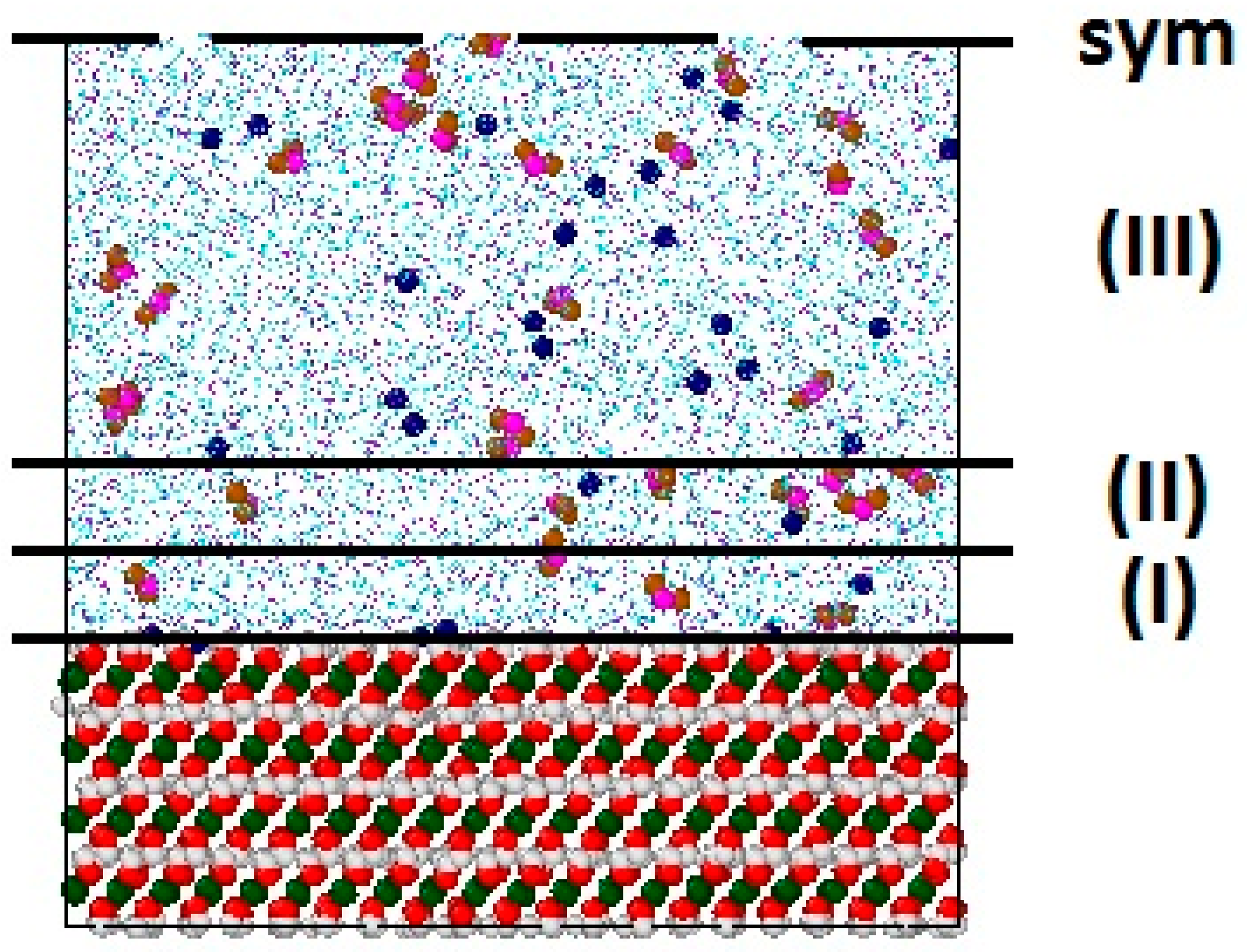
The created portlandite surfaces were brought into contact with a layer of NaNO2 aqueous solution approximately 85 Å thick. According to experimental data [32], this size is comparable to typical capillary pores in hardened cement. After the insertion of the aqueous layer, the dimensions of the simulation supercell were ~71.7 × 62.1 × 122.8 Å3. The number of H2O molecules in the nanopore corresponded to the density of the aqueous solution under ambient conditions (≈1 g/cm3). The Na+ and NO2− ions were initially uniformly distributed in the nanopore. The resulting nominal NaNO2 solution molality in the pore space was ≈0.56 mol/kg (12,632 H2O molecules and 64 ion pairs). This corresponds to the experimentally measured solution molalities in the pores in cement materials [6].
Figure 1 shows a representative snapshot fragment of the simulation supercell. For the subsequent analysis, the interfacial space occupied by the solution was subdivided into three layers. The first near-surface layer (I) starts from the average positions of hydroxyl hydrogen atoms on the portlandite surface, Hh, and has a thickness of 3.5 Å (approximately one molecular diameter of H2O. The second layer (II) immediately follows it and has the same thickness of 3.5 Å. In the rest of the pore space (III), the solution is considered to be much less affected by the surface and has properties close to those of the bulk phase.
2.2. Force Field Parameters
A series of preliminary simulations for the bulk Ca(OH)2 crystals was initially performed with both ClayFF-orig and ClayFF-MOH versions of the force field, in order to assess the relative accuracy of both versions. The MOH variation adds harmonic energy terms for Metal-O-H (M-O-H) angle bending in the crystal structure. The equilibrium angles and stiffness parameters were originally reported for Mg-O-H and Al-O-H angles [17]. They have been fitted to reproduce the lattice structure and dynamics obtained by density functional theory (DFT) calculations of brucite (Mg(OH)2)and gibbsite (Al(OH)3). The optimized parameters for Mg-O-H angles are as follows [16]: θ0,MgOH = 110° and kMgOH = 6 kcal∙mol−1∙rad−2. In this work, we use the same parameters for the Ca-O-H angles, based on the close similarity between the Mg(OH)2 and Ca(OH)2 crystal structures.
Water molecules were modeled using the flexible SPC/E model [33], and the parameters representing hydrated Na+ ions were taken from the updated ClayFF model [16]. As mentioned above, we used here a new parameterization of charges, Lennard-Jones constants, and intramolecular constants for the NO2− ions in combination with the ClayFF force field [18]. This parameterization took into account recent results of DFT calculations for the nitrite ion dissolved in water [34,35], some earlier NO2− models use in classical MD simulations [36,37,38], and experimental data [39]. All force field parameters used in this work were specifically parametrized to be consistent with the same SPC/E water model, therefore they are expected to be transferable and provide reliable results in the simulations of other systems that are consistent with the same model of water, as has been already demonstrated numerous times in the ClayFF-based simulations of various nanoporous and layered materials and their aqueous interfaces over the last 20 years [16].
2.3. Simulation Details
All MD simulations were performed using the LAMMPS simulation package [40]. LAMMPS is one of the most commonly used computer simulation software packages for modeling of cementitious materials and their interfaces with aqueous solutions (e.g., ref. [11]). Periodic boundary conditions in all three dimensions were used in all simulations. A cutoff radius of 12.5 Å was used for short-range forces, and the PPPM method was used to account for long-range electrostatic interactions [41,42]. The GPU accelerator within the LAMMPS package was used to speed up the calculations [42,43]. Standard Lorentz-Berthelot mixing rules () were applied to calculate the Lennard-Jones parameters of interaction between unlike atoms [16,41]. The Newtonian equations of motion were numerically integrated with a time step of 0.5 fs via the velocity–Verlet algorithm [41,44].
The constructed models were initially equilibrated for 1 ns at the temperature of 298 K and pressure of 1 bar using the Nose-Hoover thermo-barostat [41,45,46]. After the equilibration in the NPT statistical ensemble (constant number of particles, constant temperature, and constant pressure), the equilibrium simulation run was performed in the NVT statistical ensemble (constant number of particles, constant temperature, and constant volume) using the Nose-Hoover thermostat [41,45,46]. The equilibrium NVT part was also 1.0 ns long and the generated equilibrium dynamic trajectories of atoms were then used for further statistical analysis.
The quantitative analysis of the structure, dynamics, and energetics of the portlandite-solution interfaces was performed following the standard approaches that are commonly used for such kinds of interfacial simulations (e.g., ref. [47]).
3. Results and Discussion
3.1. Bulk Portlandite Properties
3.1.1. Crystallographic and Structural Parameters
Table 1 shows the equilibrium parameters of the crystallographic unit cell of portlandite calculated with the ClayFF-orig and ClayFF-MOH versions of the force field, in comparison with experimental data [24,48], DFT calculations [26,49,50], and earlier results of classical MD simulations [11,51,52,53,54]. In our simulations, all unit cell parameters were optimized in the NPT ensemble MD runs without any symmetry constraints.
The results clearly reproduced the hexagonal crystal structure, in agreement with experimental data, and the discrepancy of lattice parameters did not exceed 2.4% for the ClayFF-MOH version. Both versions of the ClayFF force field also showed a good agreement with the DFT results. There were no significant differences in the crystallographic parameters between the ClayFF-orig and ClayFF-MOH models, indicating that introducing the explicit M-O-H angle bending terms in portlandite does not affect the symmetry of the crystal. One has to note, however, that this agreement is not particularly surprising because portlandite was one of the model structures used to parametrize the original ClayFF force field [20,21].
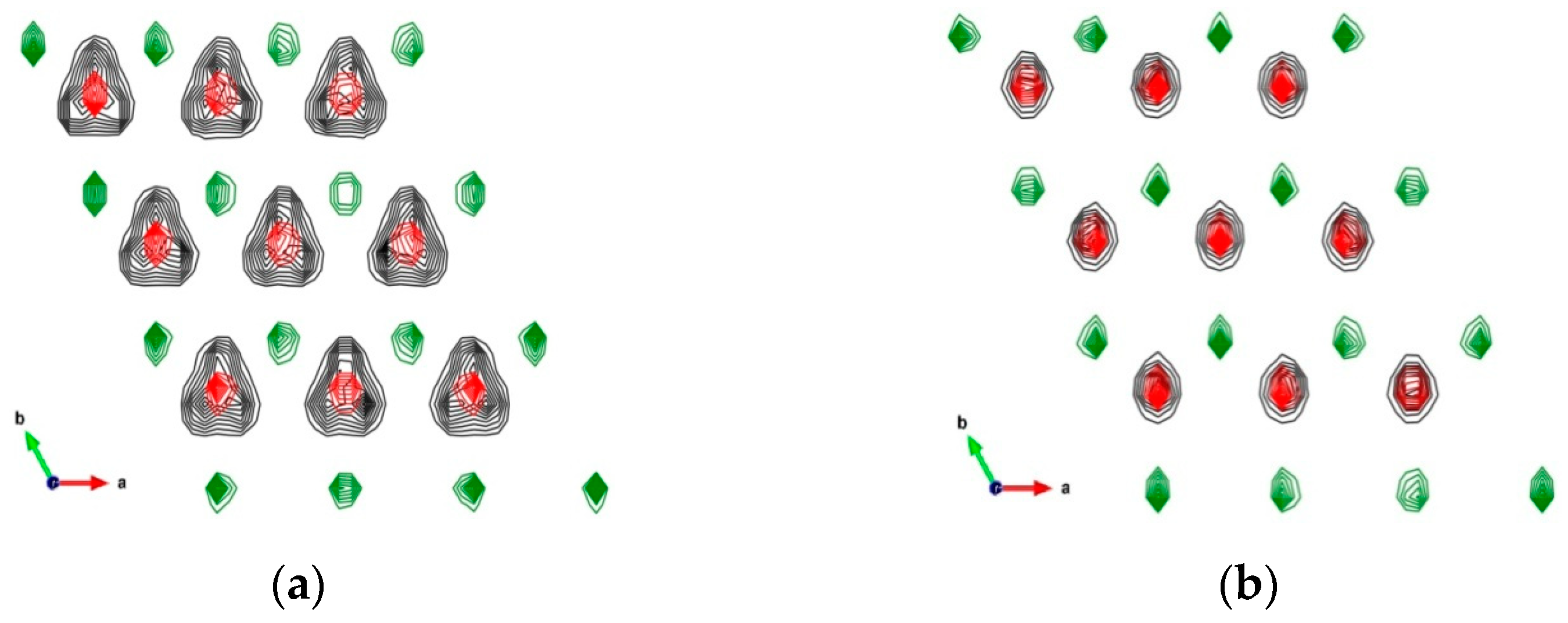
The small differences in the crystallographic parameters between the ClayFF-orig and ClayFF-MOH models are due to the much stronger localization of the hydrogen atoms and the orientation of hydroxyl groups for the latter case (Figure 2). In the case of ClayFF-orig, the hydroxyl groups are freely oriented with their hydrogen atoms, Hh, towards one of the three hydroxyl oxygen atoms, Oh, of the opposite crystal layer, forming a strong hydrogen bond. Due to the unconstrained Ca-O-H angle in the ClayFF-orig, the hydroxyl groups can frequently and freely rotate, and those hydrogen bonds switch between three Oh atoms from the opposite layer. Such poorly constrained rotations of hydroxyl groups lead to a slight expansion of the interlayer space. Consequently, the parameter c of the portlandite unit cell increased, and the parameters a and b decreased compared to the ClayFF-MOH. As Figure 2a shows, the Hh atoms in the ClayFF-orig model can be oriented with equal probability in all three directions, corresponding to the locations of the Oh atoms in the neighboring layer (Oh atoms of the opposite layer are not shown).
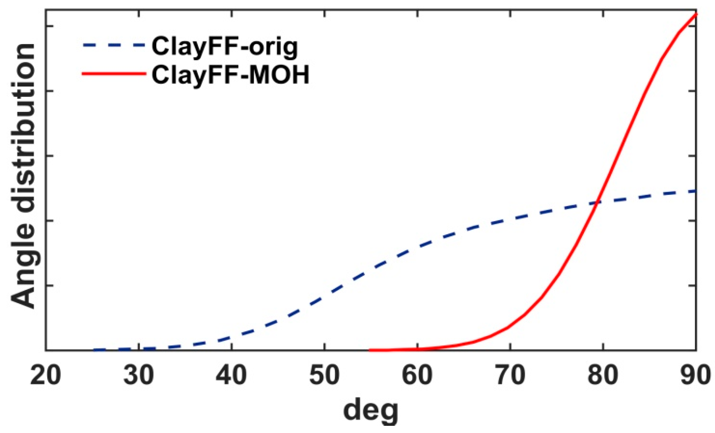
Figure 2b demonstrates a much stronger localization of Hh atoms in the ClayFF-MOH model. Figure 3 shows the distributions of angles of hydroxyl groups to the ab plane in the original and ClayFF-MOH versions, which also reflect a more disordered behavior of hydroxyls in ClayFF-orig. In contrast, the hydroxyl O-H bonds are more strongly localized around the normal to the ab plane in the ClayFF-MOH model. According to the DFT results, such localized behavior of hydroxyls is more realistic of brucite-like materials [17] and is in better agreement with experimental data [22].
3.1.2. Power Spectra of Atomic Vibrations in Portlandite Crystals
Analysis of atomic vibration spectra in the crystal gives further insights into the dynamics of portlandite hydroxyls. Figure 4 shows smoothed power spectra reflecting the vibrations in the ab crystallographic plane for all portlandite atoms and, separately, the contribution of Hh-atoms calculated in both versions of ClayFF. The smoothing of the spectra was carried out by applying the exponential damping with the characteristic time τdamp = 0.25 ps to the velocity autocorrelation functions, as proposed by Szczerba et al. [55].
The low-frequency region of the spectrum corresponds to the librational modes of the hydroxyl groups and to the lattice vibrations. In the ClayFF-orig model, the individual peaks were unresolved and all merged into one single wide spectral band. In the ClayFF-MOH model, the individual peaks were better resolved for both libration and lattice vibration modes, which is in a better qualitative agreement with the vibrational behavior of portlandite crystal observed in experiments [56] and DFT calculations [50], compared to the ClayFF-orig model.
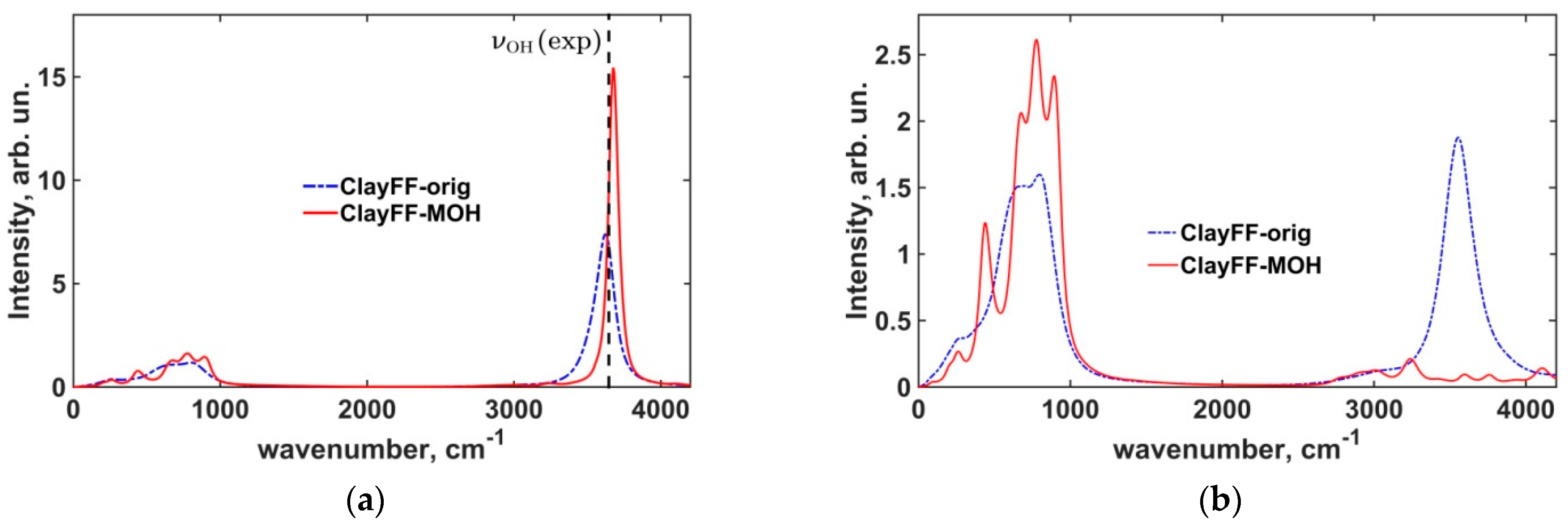
The most noticeable differences between the two versions of ClayFF in Figure 4a,b are in the high-frequency range of the spectra. The peaks corresponding to the O–H stretching modes of hydroxyls are located at positions 3624 cm–1 and 3676 cm–1 for the ClayFF-orig and ClayFF-MOH models, respectively. For the ClayFF-MOH, the peak frequency is slightly higher than the experimental data [56,57,58], where the O–H stretching peaks are located at 3620 cm–1 (A1g mode) and 3646 cm–1 (A2u mode) for Raman and IR spectroscopy, respectively. The lower frequency of the O–H stretching peak in the ClayFF-orig compared to the ClayFF-MOH indicates that the interlayer hydrogen bonding is stronger in the former model. As mentioned above, in the ClayFF-orig, Hh atoms instantaneously bond with only one opposite-layer Oh atom. In ClayFF-MOH, an Hh atom can participate in up to 3 weaker hydrogen bonds at the same time, due to the higher localization of Hh atoms in the structure. For instance, in brucite under normal conditions, the preferred orientation of the hydroxyl groups is along the normal to the magnesium octahedral layer [17,59]. The reorientation of hydroxyl groups in brucite and portlandite towards the opposite-layer Oh atoms occurs only at high temperatures and pressures [23,60]. This exaggerated reorientation of hydroxyls under normal conditions in the ClayFF-orig model is especially noticeable in the isolated spectrum of Hh-atoms in the ab crystallographic plane, where a very strong peak is observed in the high-frequency region, as seen in Figure 4b.
3.2. Properties of Portlandite-NaNO2 Aqueous Solution Interfaces
3.2.1. Structural Properties of Interfacial Solutions
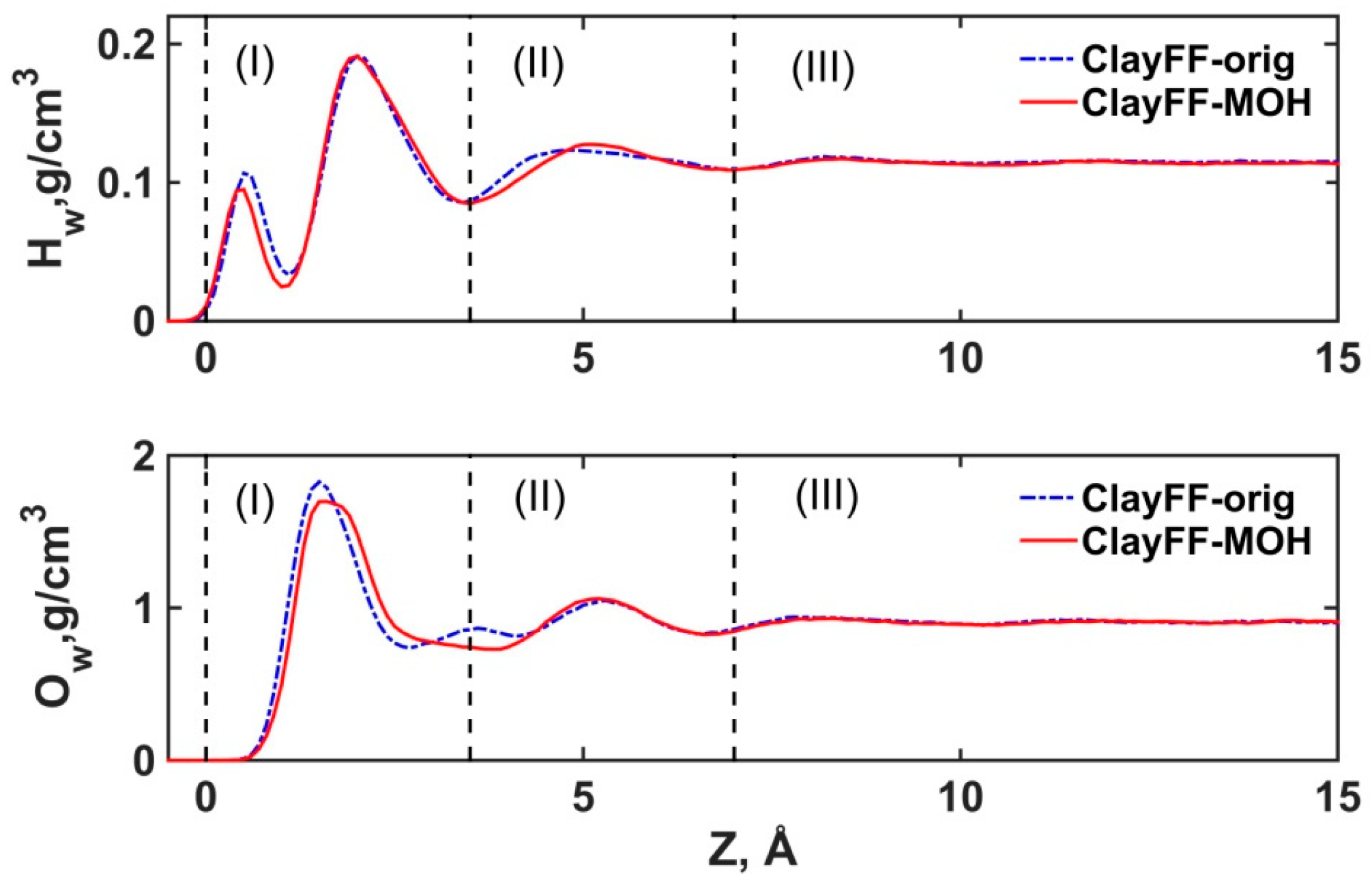
First, we discuss the structural differences in the simulated aqueous solution between the two ClayFF versions. Figure 5 shows atomic density profiles of Hw and Ow atoms of the H2O molecules along the direction normal to the portlandite surface for both versions of ClayFF. As expected for the ClayFF-orig version, the profiles for Hw and Ow were similar to the earlier MD simulation results with this force field [20,51]. However, slightly different profiles are observed with the ClayFF-MOH model, indicating some changes in the local interfacial solution structure. Below, we argue that the reason for the changes in the density profiles in the first two solution layers, (I) and (II) (as defined in Figure 1) are directly related to very specific interfacial molecular coordinations.
DFT and MD results show that one of the most probable orientations of the H2O molecule dipole vector is 170–175° with respect to the surface normal [26,51]. With this orientation, the H2O molecule donates two hydrogen bonds to the Oh atoms of the hydroxyls on the surface of the crystalline phase and this orientation of the H2O molecule corresponds to the bidentate coordination towards the surface [55]. In addition, there may be a monodentate coordination with the dipole vector oriented ≈90° to the surface normal [55]. Such orientations of H2O molecules on the (001) surface of portlandite have been reported in other recent MD simulations [61]. Due to the more accurately constrained vertical orientations of the surface hydroxyl groups with the ClayFF-MOH model, H2O molecules in those two orientations are adsorbed closer to the portlandite surface. That, in turn, results in stronger hydrogen bonds in the donor-acceptor pairs Hw···Oh and Hh···Ow. The stronger bonding of H2O molecules in mono- and bidentate orientations is reflected in the shift of the first peak of the Hw profile closer to the portlandite surface (in layer (I)) compared to the ClayFF-orig version.
However, the Ow and Hw interfacial density profiles for both versions of the force field clearly reproduce the distinct layering of water at least within the first two molecular layers, which is fully consistent with the results of previous simulations [20,51,61] and justifies our definition of the solution layers in Figure 1.
The slight shift of the first minimum of the Hw profile in layer (I) for ClayFF-MOH (Figure 5) is also explained by the adsorption of the H2O molecules closer to the portlandite surface. The second peaks of the density profiles in layer (I) are located at the same positions for both versions of the ClayFF model. These peaks are the highest and correspond to the most common orientation of H2O molecules, in which interfacial H2O molecules accept hydrogen bonds from surface hydroxyls (donor-acceptor pair Hh···Ow) and H2O molecules are located along the hydroxyl O-H bonds. In the second layer (II), the Hw density maximum shifts away from the surface for the ClayFF-MOH model compared to ClayFF-orig. The reason for this is that the mono- and bidentate-oriented H2O molecules in layer (I) are coordinating the H2O molecules from layer (II) in a slightly different manner due to more stable hydrogen bonds with the surface observed with the ClayFF-MOH model. These changes are reflected in the Ow profiles as well, where there are two peaks In the near-surface layer (I) and (II) for the ClayFF-MOH compared to three peaks for the ClayFF-orig. The broadening of the first peak and the absence of a peak at the boundary of layers (I) and (II) In ClayFF-MOH indicate the formation of a stronger hydrogen bonding network on the surface of portlandite. In general, the H2O atomic density profiles for the ClayFF-MOH are qualitatively more similar to the H2O profiles from the MD simulations with a more optimized force field for solid and a four-point TIP4P/2005 water model [61].
Thus, the ClayFF-MOH model provides a better qualitative and quantitative description of the portlandite crystal and the portlandite-water interface. Therefore, in the rest of the paper, the behavior of dissolved ions and H2O molecules on the portlandite surface are presented and discussed only for the ClayFF-MOH model.
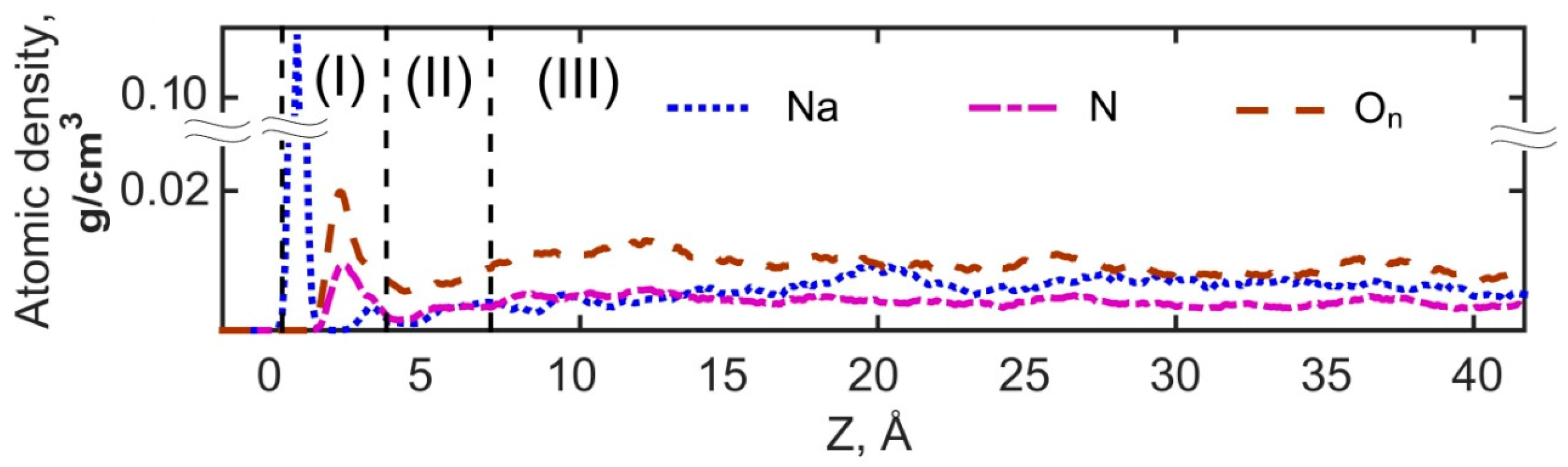
Figure 6 shows the density profiles of Na+ ions and N and On atoms of NO2− in the sodium nitrite aqueous solution next to the portlandite surface. The density profile of Na+ is similar to the previously reported profiles [20,51] with Na+ is mainly adsorbed with inner-sphere surface coordination. Inner-sphere coordination is also observed for adsorbed NO2− ions, as the first density peaks of N and On are located within layer (I) of the solution at distances of 2.1 and 2.0 Å from Hh, respectively. The first minima of the profiles are located in both cases within the layer (II) of solution at distances of 4.0 Å for N and 4.1 Å for On, indicating that adsorbed NO2− ions can be oriented both with their N and On atoms towards the Hh hydroxyls. In both orientations NO2− ions accept hydrogen bonds from surface hydroxyls.
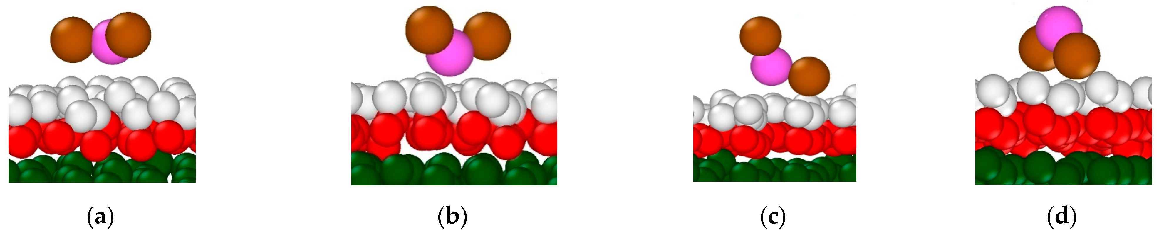
Visual analysis of the trajectories with the OVITO package [62] has shown that the adsorbed NO2− ions demonstrate four main types of surface coordination as illustrated in Figure 7a–d. In the first coordination (Figure 7a), all three atoms of the NO2− ion are in a plane oriented almost parallel to the portlandite surface and coordinated by surface hydroxyls. The other three orientations have only the N atom, one On atom, or both On atoms coordinated by the surface hydroxyls, as shown in Figure 7b, Figure 7c and Figure 7d, respectively. These types of coordination can be seen for the anions adsorbed next to Na+ ions on the surface as well as for the anions located far from adsorbed cations. As mentioned above, the first minima of the N and On density profiles are located within the solution layer (II), so that the density of NO2− in that layer is lower than in layer (I) and in layer (III) that reflects bulk solution properties. This behavior of NO2− in layer (II) is caused by the repulsion from the first NO2− adsorption layer in layer (I).
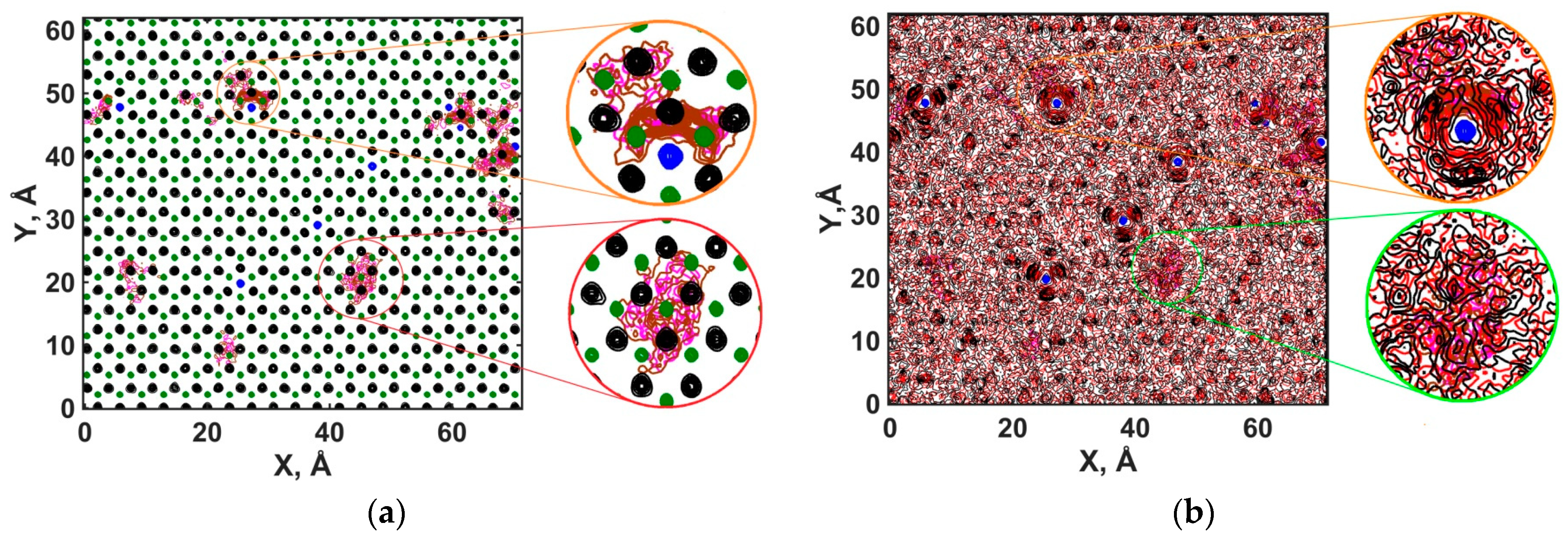
The surface distribution of molecules visualized by atomic density contour maps for the solution layer (I) shows that Na+ ions are adsorbed at the centers of triangles formed by Oh atoms, as illustrated in Figure 8. The inner-sphere adsorption of Na+ ions and the coordination of the H2O molecules around them by Ow atoms agrees well with the previous MD results [20,51]. Unlike Hu et al. [63], we did not observe the preference of NO2− adsorption surrounding the cations and forming surface clusters. Instead, NO2− ions can be adsorbed both near Na+ and far from them. In both cases, the adsorbed anions are quite strongly bound to the surface and do not change their binding site within the time scale of the simulation. Nevertheless, the nitrite anions frequently change their orientation while staying at the same surface adsorption site. Due to the frequent changes of adsorbed NO2− ions orientation, the H2O molecules that form hydrogen bonds with these NO2− ions did not have any predominant coordination type, as seen in Figure 8b.
3.2.2. Power Spectra of the Interfacial Dynamics
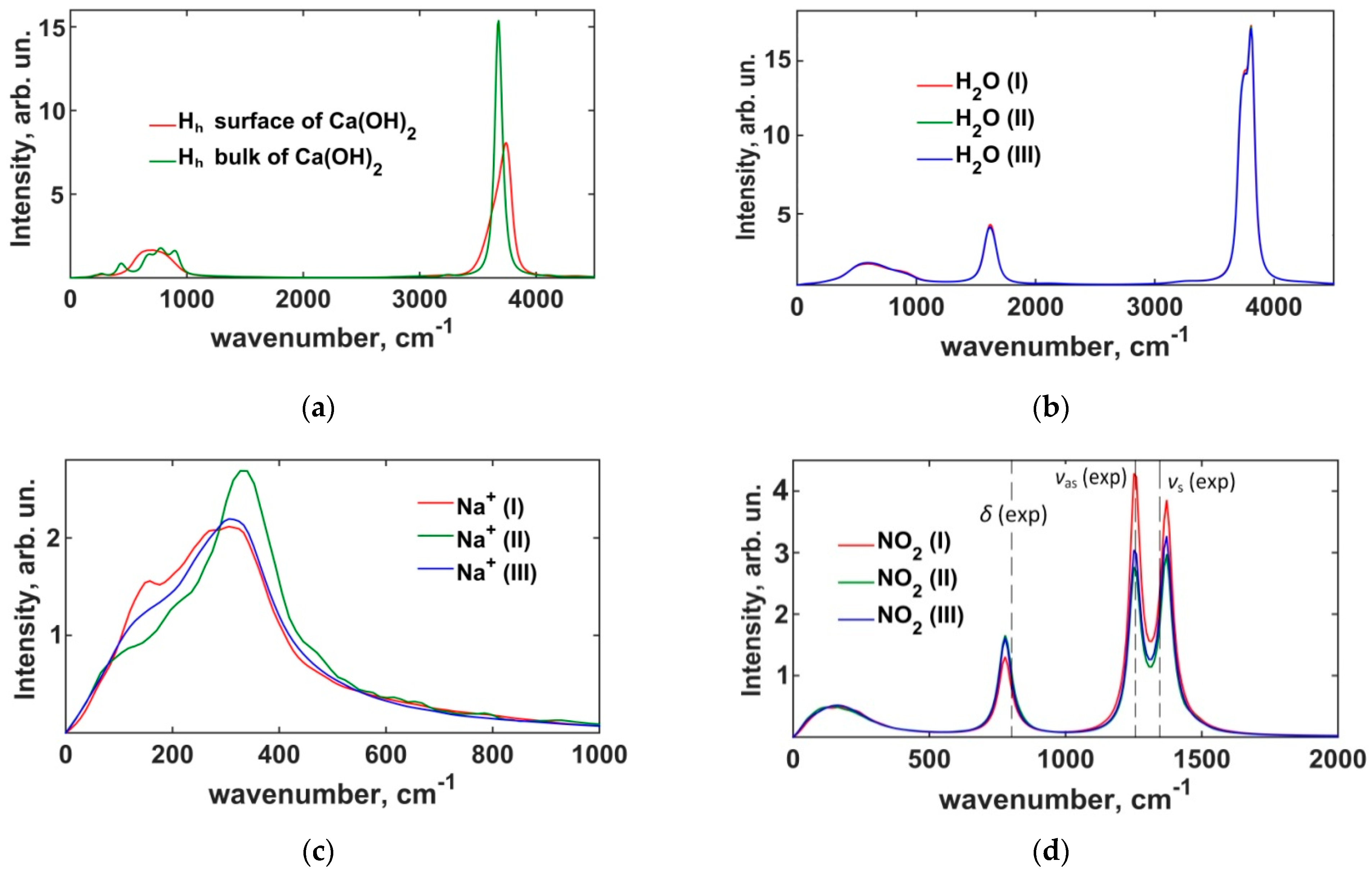
Power spectra reflecting the vibrations of Hh atoms at the surface and in the bulk structure of portlandite are shown in Figure 9a. As mentioned in Section 3.1.2, the low-frequency region of the bulk portlandite spectrum has a band where several peaks can be resolved. In contrast to that, only two peaks can be resolved in that band for surface Hh, which indicates a superposition of normal vibration modes for surface hydroxyls. In the high-frequency range, the peak corresponding to the stretching of O–H bonds is broader, less intense, and significantly blue-shifted (3676 cm–1 vs. 3743 cm–1) for surface hydroxyls compared to the bulk phase, which is typical for surfaces of brucite-like minerals [59]. The shift of the O–H stretching vibrations peak for surface Hh at the crystal–solution interface is significantly smaller than with the crystal-vacuum interface [59]. The reduced peak shift is due to the formation of hydrogen bonds of the surface hydroxyls with the Interfacial H2O molecules and NO2− ions. Figure 9b shows that the power spectra of the H2O solution molecules at all distances from the surface are identical. This may merely reflect the fact that simple harmonic potentials used here to model the intramolecular vibrations in the SPC/E water model are not accurate enough, and more complex inharmonic models are necessary (see, e.g., ref. [55]). However, the libration, bending, and stretching modes of H2O molecules are reproduced with only small deviations from the experimental data [64,65].
Unlike the case with H2O molecules, the spectra reflecting the surface dynamics of Na+ ions show some dependence on the distance from the surface, as seen in Figure 9c, which confirms the previous MD results [20], where such spectra have been analyzed in detail. However, the NO2− power spectra in different solution layers have peaks at the same frequencies, differing only in magnitudes, as shown in Figure 9d. The positions of the spectral peaks are in good agreement with the results of Raman spectroscopy [39]: the calculated frequency of the bending mode, δ, is at 779 cm–1, compared to 817 cm–1 from the Raman spectroscopy. The calculated asymmetric, νas, and symmetric, νs, N-On stretching modes peaks are at 1250 cm–1 and 1371 cm–1, respectively, compared to the experimentally determined values of 1242 cm–1 and 1331 cm–1.
3.2.3. Structure and Dynamics of the Interfacial Hydrogen Bonding
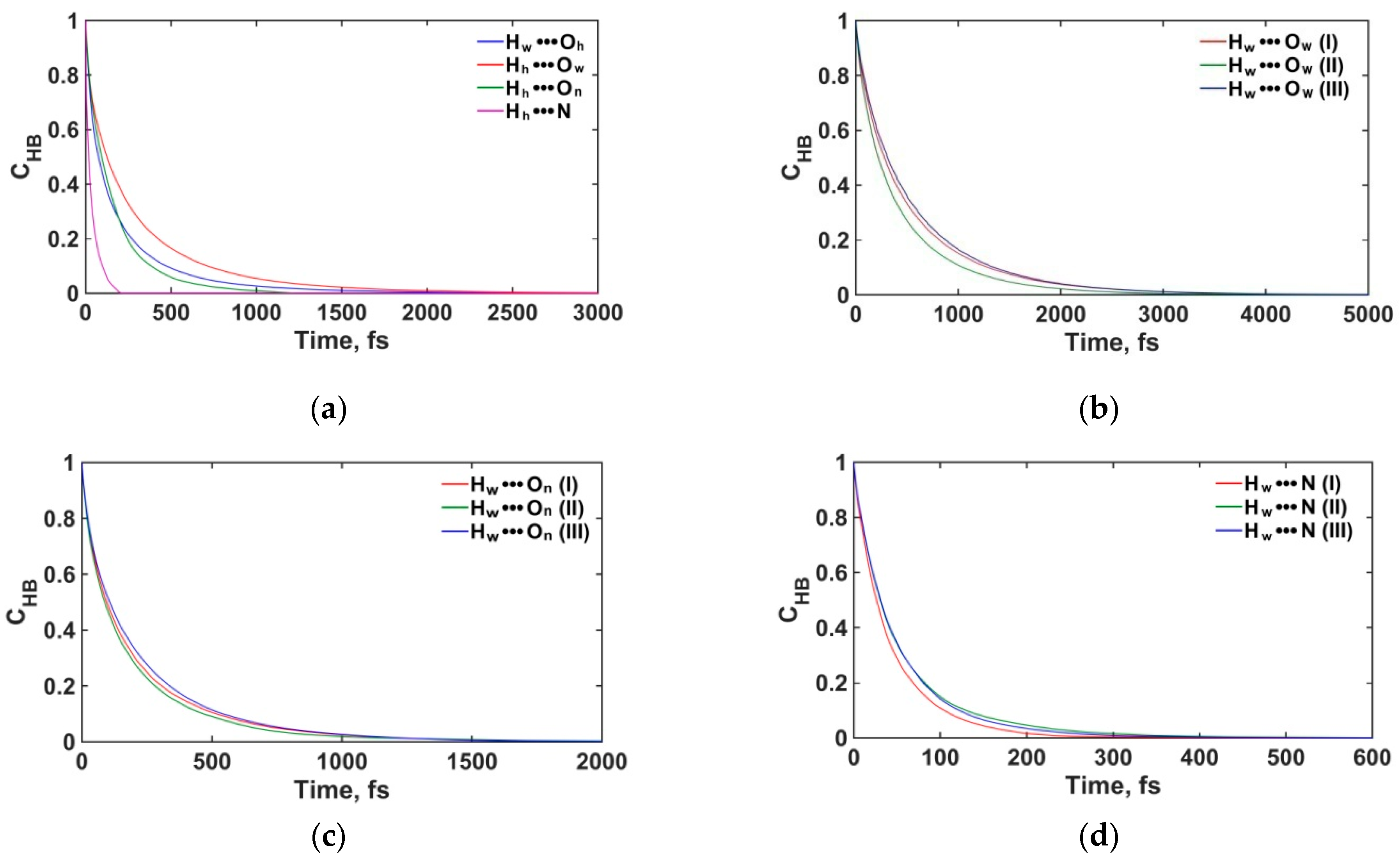
To better characterize the structural and dynamic properties of the interfacial solution, we have also studied the dynamics of hydrogen bonds (H-bonds), which were formally defined using a common geometric criterion: an H-bond between a hydrogen Hw (donor) and oxygen Ow (acceptor) atoms of two H2O molecules was assumed to exist if the Hw···Ow distance is less than 2.45 Å and the angle between the H-bond direction and the vector connecting the Ow atoms of the donor and acceptor molecules is less than 30° (e.g., ref. [66]). For H-bonds between H2O molecules and NO2− (Hw···N and Hw···On pairs), the distance thresholds were taken according to [35]: RHw-N ≤ 2.25 Å and RHw-On ≤ 2.35 Å. The geometrical definitions for H-bonds between portlandite surface hydroxyls and H2O (or NO2−) were taken to be the same as for H2O molecules (or H2O and NO2−) in solution. The average lifetimes τHB for various types of H-bonds were then assessed by integrating the so-called continuous-time autocorrelation functions [35,66,67,68] as illustrated in Figure 10. In addition, the average number of hydrogen bonds nHB per H2O molecule and acceptors N and On were also calculated.
It was found that the portlandite hydroxyls form the most stable H-bonds with the H2O molecules of the solution (pairs Hh···Ow and Hw···Oh). The lifetime of the Hh···Ow bonds is longer than that for Hw···Oh, despite the fact that in the ClayFF model, the charge of Oh is more negative than that of Ow, while the charges of Hh atoms and Hw atoms in SPC/E are almost equal. In the bidentate orientation of H2O molecules, which is most preferable on the surface of portlandite [26], H2O molecules are also coordinated by neighboring hydroxyls (Hh···Ow pairs) without forming hydrogen bonds between Hw and Oh of this hydroxyls.
As mentioned above, monodentate orientation can also occur, in which H-bonds between the Hh···Ow and Hw···Oh pairs are formed. Therefore, a significant role on the hydrated (001) portlandite surface is played by the H-bonds donated by the hydrogen atoms of the surface hydroxyl groups to the oxygen atoms of H2O molecules (pair Hh···Ow), which inhibits the penetration of H2O molecules closer to the portlandite surface and the dissolution of calcium ions [29].
Table 2 shows that the lifetime of H-bonds between H2O molecules in the solution layer (I) is longer than in the layer (II), while the number of H-bonds per H2O molecule remains about the same for both near-surface layers. This means that the interaction of H2O molecules with surface hydroxyls orients them in a way that favors the formation of a more stable H-bond network between themselves in layer (I). That H-bonding network of the H2O molecules nearest to the surface (in layer (I)) creates an ice-like two-dimensional layer on the surface of portlandite [29]. In the bulk solution (layer (III)), the number of H-bonds per H2O molecule and the bond lifetime have typical values for low-concentration aqueous solutions [69].
For interactions between water molecules and nitrite ions, the H-bonds Hw···On are stronger than Hw···N, which is consistent with the DFT results for hydrated NO2− [35]. The H-bonds for these pairs have approximately the same lifetimes in all layers of the aqueous solution. However, the average number of H-bonds per acceptor atom in Hw···N pairs in layer (I) is lower than in layer (II), because some of the H2O molecules in layer (I) bind with surface hydroxyls instead of NO2− nitrogen atoms. The lifetime of Hh···N bonds between hydroxyls and NO2− is close to the lifetime of the Hw···N bond, however, the Hh···On bonds have shorter lifetimes than Hw···On. Such a decrease in the lifetime is due to the vibrational behavior of the surface hydroxyls of the crystalline phase, which is also noticeable when comparing the lifetimes of the Hh···Ow and Hw···Ow pairs. We can also see that the H-bonds between surface hydroxyls and adsorbed NO2− ions are weaker than the ones between hydroxyls and H2O molecules. This is consistent with the absence of a strongly preferred NO2− orientation on the portlandite surface.
3.2.4. Water Molecules and Nitrite Ions Orientational Relaxation
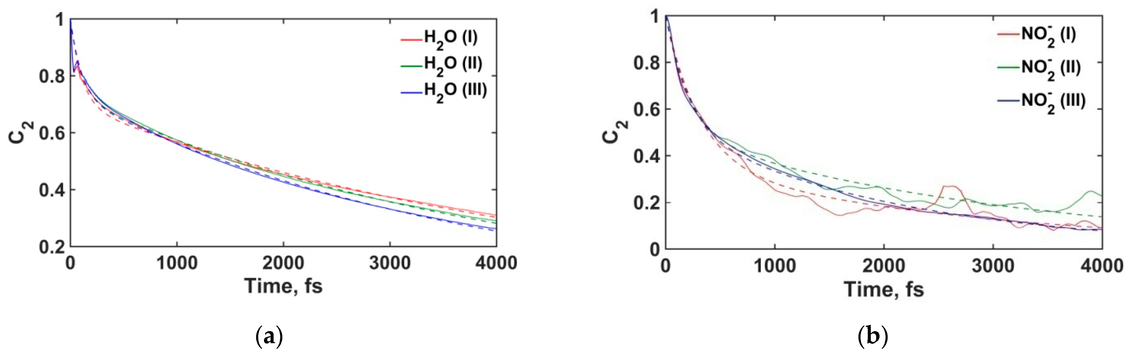
The orientational relaxation of NO2− ions and H2O molecules can be characterized using the autocorrelation function of the unit vectors directed along the N-On or Ow-Hw bonds [35,70,71,72], which was calculated using the second-rank Legendre polynomial:
where is the linear correlation between the unit vector of bond orientation at time moments and , and angular brackets 〈…〉 denote the averaging over all molecules and over all possible initial moments along the equilibrium MD trajectory. The correlation functions of NO2− and H2O molecules in three layers of the aqueous solution are shown in Figure 11. The orientational correlation times were calculated by fitting C2 with bi-exponential functions [35]:
where the shorter time constant τ1 reflects the rotational inertia of an ion or molecule in the libration mode, which is affected by H-bonding around the ion/molecule [71]. The longer time constant τ2 characterizes the reorientation of an ion or molecule due to the rotational Brownian motion and to large angular jumps associated with the breaking of H-bonds [35,71].
Table 3 shows the orientational relaxation times for NO2− and H2O, depending on the molecule location in the pore. For H2O molecules, the time τ1 for all layers of the solution have similar values, indicating low sensitivity of librational molecular motions to the variation of local H-bonding environment between bulk solution and near-surface layers. The power spectra in Figure 9b also indicate the same behavior in the low-frequency region. On the other hand, the time τ2 for H2O molecules increases in the near-surface layers. Such an increase in rotational relaxation time confirms the aforementioned formation of a more stable H-bonding network at the surface of crystalline portlandite due to hydroxyl group–water interactions.
The increase in τ2 near the surface compared to their bulk solution values is seen for NO2− ions as well, which is also due to the participation of the nitrite ions in the more stable H-bonding network at the surface of portlandite. In the closest near-surface layer, we also observe an increase in time τ1, indicating that the NO2− ion adsorption affects its libration modes.
3.2.5. Diffusional Mobility of Water and Ions at the Portlandite Surface
The translational dynamics of NO2−, Na+, and H2O molecules in the near-surface layers and in the bulk of the solution were studied by calculating the self-diffusion coefficients of these species using the Einstein–Smoluchowski relation [41,72,73]. For H2O molecules, we calculated the 3-dimensional (3d) diffusion coefficients separately for the solution layers (I), (II), and (III), as defined in Figure 1. For the ions, due to their relatively small number in the simulated systems, only bulk (layer (III)) 3-dimensional diffusion coefficients were calculated.
Table 4 shows the calculated self-diffusion coefficients. The average self-diffusion coefficients for the ions are found to be = (0.84 ± 0.17) × 10–5 cm2/s, = (1.46 ± 0.16) × 10–5 cm2/s. The calculated diffusivities of ions in water are lower than the experimental values = 1.33 × 10⁻⁵ cm2/s and = 1.91 × 10⁻⁵ cm2/s [74].
The diffusional mobility of water molecules decreases as they approach the surface, with = (1.81 ± 0.16) × 10–5 cm2/s, = (1.47 ± 0.18) × 10–5 cm2/s, and = (1.36 ± 0.21) × 10–5 cm2/s. The diffusivity of water in the bulk layer is underestimated compared to the experimental data = 2.33 × 10⁻⁵ cm2/s [75]. The reduced calculated diffusivities of water and ions reflect the effect of their interactions with the portlandite surface but are also partly due to the known underestimation of the molecular mobility by the flexible SPC/E model and due to the finite size effects of the periodic boundary conditions [76].
4. Conclusions
The recently modified ClayFF force field, ClayFF-MOH [10], with added Ca-O-H angular bending terms, together with a new parameterization for NO2− ions [18] were used to study the structure and dynamics of sodium nitrite solutions at the surface of portlandite using classical MD simulations. The (001) crystal surface of portlandite was selected for these simulations because it is the least reactive when interacting with water compared to other surfaces. We show that the inclusion of the Ca-O-H bending term does not affect the simulation results for the crystal structure but does affect the vibrational properties of the crystal, bringing them closer to the experimental data. This, in turn, affects the structural properties of the aqueous solutions in the near-surface layers due to the increased localization of surface hydroxyl groups of portlandite.
The better-constrained orientation of the hydroxyls on the (001) surface of portlandite leads to a more realistic description of the hydrogen bonds formed between surface hydrogen atoms and water molecules (Hh···Ow donor-acceptor pair), facilitating the formation of a network of H-bonds between water molecules themselves, which form a surface layer inhibiting the dissolution of calcium ions into water. The formation of the interfacial H-bonding network manifests itself in the increase in the rotational relaxation time for water molecules near the portlandite surface.
Despite the formation of the water-water H-bonding network on the surface of the crystalline phase, the surface can adsorb dissolved nitrite and sodium ions. We show that the adsorption of nitrite ions involves the formation of H-bonds donated by surface hydroxyls not only to the oxygen atoms of NO2−, but also to the nitrogen atoms, i.e., both Hh···On and Hh···N donor-acceptor pairs are present. Although the H-bonds Hh···On and Hh···N are weaker than the H-bonds Hh···Ow donated to the water molecules, NO2− ions infiltrate the H-bonding network on the surface of portlandite and are quite strongly adsorbed at it with no visible translational diffusion over the timescale of the entire MD simulation (~1 ns). On the other hand, the orientation of the adsorbed ions can change over time, so that there is no single preferred coordination of the adsorbed NO2− to the surface, meaning that the H-bonds in the Hh···On and Hh···N pairs are less stable and can frequently break and re-form. The NO2− ions can be adsorbed onto the surface of portlandite next to the previously adsorbed Na+ ions as well as separately without any strong association with the cations.
Author Contributions
Conceptualization, A.G.K. and E.V.T.; methodology, A.G.K. and V.V.P.; investigation, E.V.T.; data analysis E.V.T., V.V.P. and A.G.K.; writing—original draft preparation, E.V.T.; writing—review and editing, E.V.T., V.V.P. and A.G.K.; visualization, E.V.T.; supervision, V.V.P. and A.G.K.; project administration, V.V.P. and A.G.K.; funding acquisition, E.V.T., V.V.P. and A.G.K. All authors have read and agreed to the published version of the manuscript.
Funding
This study was sponsored by Agence Nationale pour la Gestion des Déchets Radioactifs and National Research University Higher School of Economics.
Institutional Review Board Statement
Not applicable.
Informed Consent Statement
Not applicable.
Data Availability Statement
All data are available from the authors upon request.
Acknowledgments
The article was prepared within the framework of the HSE University Basic Research Program and was supported by computational resources of HPC facilities at HSE University [77,78]. A.G.K. also acknowledges the financial support of the industrial chair “Storage and Disposal of Radioactive Waste” at the IMT Atlantique, funded by ANDRA, Orano, and EDF.
Conflicts of Interest
The authors declare no conflict of interest.
References
- Phair, J.W. Green chemistry for sustainable cement production and use. Green Chem. 2006, 8, 763–780. [Google Scholar] [CrossRef]
- Rosemberg, A.M.; Gaidis, J.M. Mechanism of nitrite inhibition of chloride attack on reinforcing steel in alkaline aqueous environments. Mater. Perform. 2004, 18, 45–48. [Google Scholar]
- Schießl, P.; Moersch, J. Effectiveness and harmlessness of calcium nitrite as a corrosion inhibitor. In Proceedings of the International RILEM Conference on the Role of Admixtures in High Performance Concrete, Monterrey, Mexico, 21–26 March 1999; RILEM Publications SARL: Paris, France, 1999; pp. 169–182. [Google Scholar]
- Nmai, C.K. Cold weather concreting admixtures. Cem. Concr. Compos. 1998, 20, 121–128. [Google Scholar] [CrossRef]
- Yoneyama, A.; Choi, H.; Inoue, M.; Kim, J.; Lim, M.; Sudoh, Y. Effect of a nitrite/nitrate-based accelerator on the strength development and hydrate formation in cold-weather cementitious materials. Materials 2021, 14, 1006. [Google Scholar] [CrossRef]
- Tritthart, J.; Banfill, P.F.G. Nitrite binding in cement. Cem. Concr. Res. 2001, 31, 1093–1100. [Google Scholar] [CrossRef]
- Vollpracht, A.; Lothenbach, B.; Snellings, R.; Haufe, J. The pore solution of blended cements: A review. Mater. Struct. 2015, 49, 3341–3367. [Google Scholar] [CrossRef] [Green Version]
- Pu, Q.; Yao, Y.; Wang, L.; Shi, X.; Luo, J.; Xie, Y. The investigation of pH threshold value on the corrosion of steel reinforcement in concrete. Comp. Concr. 2017, 19, 257–262. [Google Scholar] [CrossRef]
- Scrivener, K.L.; Kirkpatrick, R.J. Innovation in use and research on cementitious material. Cem. Concr. Res. 2008, 38, 128–136. [Google Scholar] [CrossRef]
- Sanchez, F.; Sobolev, K. Nanotechnology in concrete—A review. Cons. Build. Mat. 2010, 24, 2060–2071. [Google Scholar] [CrossRef]
- Mishra, R.K.; Mohamed, A.K.; Geissbühler, D.; Manzano, H.; Jamil, T.; Shahsavari, R.; Kalinichev, A.G.; Galmarini, S.; Tao, L.; Heinz, H.; et al. CemFF: A force field database for cementitious materials including validations, applications and opportunities. Cem. Concr. Res. 2017, 102, 68–89. [Google Scholar] [CrossRef] [Green Version]
- Lasich, M. Sorption of natural gas in cement hydrate by Monte Carlo simulation. Eur. Phys. J. B 2018, 91, 299. [Google Scholar] [CrossRef]
- Pellenq, R.J.M.; Kushima, A.; Shahsavari, R.; Van Vliet, K.J.; Buehler, M.J.; Yip, S.; Ulm, F.J. A realistic molecular model of cement hydrates. Proc. Natl. Acad. Sci. USA 2009, 106, 16102–16107. [Google Scholar] [CrossRef]
- Tavakoli, D.; Tarighat, A. Molecular dynamics study on the mechanical properties of Portland cement clinker phases. Comput. Mater. Sci. 2016, 119, 65–73. [Google Scholar] [CrossRef]
- Bahraq, A.A.; Al-Osta, M.A.; Al-Amoudi, O.S.B.; Obot, I.B.; Maslehuddin, M.; Saleh, T.A. Molecular simulation of cement-based materials and their properties. Engineering 2022, 15, 165–178. [Google Scholar] [CrossRef]
- Cygan, R.T.; Greathouse, J.A.; Kalinichev, A.G. Advances in clayff molecular simulation of layered and nanoporous materials and their aqueous interfaces. J. Phys. Chem. C 2021, 125, 17573. [Google Scholar] [CrossRef]
- Pouvreau, M.; Greathouse, J.A.; Cygan, R.T.; Kalinichev, A.G. Structure of hydrated gibbsite and brucite edge surfaces: DFT results and further development of the ClayFF classical force field with metal-O-H angle bending terms. J. Phys. Chem. C 2017, 121, 14757–14771. [Google Scholar] [CrossRef] [Green Version]
- Tararushkin, E.V. Molecular dynamic modeling of the structural, dynamic, and vibrational properties of aqueous NaNO2. Russ. J. Phys. Chem. 2022, 96, 1439–1444. [Google Scholar] [CrossRef]
- Tararushkin, E.V.; Pisarev, V.V.; Kalinichev, A.G. Atomistic simulations of ettringite and its aqueous interfaces: Structure and properties revisited with the modified ClayFF force field. Cem. Concr. Res. 2022, 156, 106759. [Google Scholar] [CrossRef]
- Kalinichev, A.G.; Kirkpatrick, R.J. Molecular dynamics modeling of chloride binding to the surfaces of calcium hydroxide, hydrated calcium aluminate, and calcium silicate phases. Chem. Mater. 2002, 14, 3539–3549. [Google Scholar] [CrossRef]
- Cygan, R.T.; Liang, J.-J.; Kalinichev, A.G. Molecular models of hydroxide, oxyhydroxide, and clay phases and the development of a general force field. J. Phys. Chem. B 2004, 108, 1255–1266. [Google Scholar] [CrossRef]
- Desgranges, L.; Grebille, D.; Calvarin, G.; Chhor, K.; Pommier, C.; Floquet, N.; Niepce, J.C. Structural and thermodynamic evidence of a change in thermal motion of hydrogen atoms in Ca(OH)2 at low temperature. J. Phys. Chem. Sol. 1994, 55, 161–166. [Google Scholar] [CrossRef]
- Schaack, S.; Depondt, P.; Huppert, S.; Finocchi, F. Quantum driven proton diffusion in brucite-like minerals under high pressure. Sci. Rep. 2020, 10, 8123. [Google Scholar] [CrossRef] [PubMed]
- Busing, W.R.; Levy, H.A. Neutron diffraction study of calcium hydroxide. J. Chem. Phys. 1957, 26, 563–568. [Google Scholar] [CrossRef]
- Galmarini, S.; Aimable, A.; Ruffray, N.; Bowen, P. Changes in portlandite morphology with solvent composition: Atomistic simulations and experiment. Cem. Concr. Res. 2011, 41, 1330–1338. [Google Scholar] [CrossRef] [Green Version]
- Mutisya, S.M.; Kalinichev, A.G. Carbonation reaction mechanisms of portlandite predicted from enhanced Ab Initio molecular dynamics simulations. Minerals 2021, 11, 509. [Google Scholar] [CrossRef]
- Harutyunyan, V.S. Adsorption energy of stoichiometric molecules and surface energy at morphologically important facets of a Ca(OH)2 crystal. Mater. Chem. Phys. 2012, 134, 200–213. [Google Scholar] [CrossRef]
- Harutyunyan, V.S. Inhomogeneity, anisotropy, and size effect in the interfacial energy of Ca(OH)2 hexagonal-prism shaped nanocrystals in water. Mat. Chem. Phys. 2014, 147, 410–422. [Google Scholar] [CrossRef]
- Salah Uddin, K.M.; Izadifar, M.; Ukrainczyk, N.; Koenders, E.; Middendorf, B. Dissolution of portlandite in pure water: Part 1 molecular dynamics (MD) approach. Materials 2022, 15, 1404. [Google Scholar] [CrossRef] [PubMed]
- Izadifar, M.; Ukrainczyk, N.; Salah Uddin, K.M.; Middendorf, B.; Koenders, E. Dissolution of portlandite in pure water: Part 2 atomistic kinetic Monte Carlo (KMC) approach. Materials 2022, 15, 1442. [Google Scholar] [CrossRef]
- Gardeh, M.G.; Kistanov, A.A.; Nguyen, H.; Manzano, H.; Cao, W.; Kinnunen, P. Exploring mechanisms of hydration and carbonation of MgO and Mg(OH)2 in reactive magnesium oxide-based cements. J. Phys. Chem. C 2022, 126, 6196–6206. [Google Scholar] [CrossRef]
- Aili, A.; Maruyama, I. Review of several experimental methods for characterization of micro- and nano-scale pores in cement-based material. Int. J. Concr. Struct. Mater. 2020, 14, 55. [Google Scholar] [CrossRef]
- Berendsen, H.; Grigera, J.; Straatsma, T. The missing term in effective pair potentials. J. Phys. Chem. 1987, 91, 6269–6271. [Google Scholar] [CrossRef]
- Vchirawongkwin, S.; Kritayakornupong, C.; Tongraarc, A.; Vchirawongkwin, V. Hydration properties determining the reactivity of nitrite in aqueous solution. Dalton Trans. 2014, 43, 12164–12174. [Google Scholar] [CrossRef]
- Yadav, S.; Chandra, A. Solvation shell of the nitrite Ion in water: An ab initio molecular dynamics study. J. Phys. Chem. B 2020, 124, 7194–7204. [Google Scholar] [CrossRef]
- Liu, Y.; Shi, X. Molecular dynamics study of interaction between corrosion inhibitors, nanoparticles, and other minerals in hydrated cement. Trans. Res. Rec. J. Trans. Res. Board 2010, 2142, 58–66. [Google Scholar] [CrossRef]
- Richards, L.A.; Schäfer, A.I.; Richards, B.S.; Corry, B. The importance of dehydration in determining ion transport in narrow pores. Small 2012, 8, 1701–1709. [Google Scholar] [CrossRef] [Green Version]
- Ohkubo, T.; Ohnishi, R.; Sarou-Kanian, V.; Bessada, C.; Iwadate, Y. Molecular dynamics simulations of the thermal and transport properties of molten NaNO2–NaNO3 systems. Electrochemistry 2018, 86, 104–108. [Google Scholar] [CrossRef]
- Irish, D.E.; Thorpe, R.V. Raman spectral studies of cadmium–nitrite interactions in aqueous solutions and crystals. Can. J. Chem. 1975, 53, 1414–1423. [Google Scholar] [CrossRef]
- Thompson, A.P.; Aktulga, H.M.; Berger, R.; Bolintineanu, D.S.; Brown, W.M.; Crozier, P.S.; in’t Veld, P.J.; Kohlmeyer, A.; Moore, S.G.; Nguyen, T.D.; et al. LAMMPS—A flexible simulation tool for particle-based materials modeling at the atomic, meso, and continuum scales. Comp. Phys. Comm. 2022, 271, 108171. [Google Scholar] [CrossRef]
- Allen, M.P.; Tildesley, D.J. Computer Simulation of Liquids, 2nd ed.; Oxford University Press: New York, NY, USA, 2017. [Google Scholar] [CrossRef]
- Brown, W.M.; Kohlmeyer, A.; Plimpton, S.J.; Tharrington, A.N. Implementing molecular dynamics on hybrid high performance computers—Particle-particle particle-mesh. Comp. Phys. Comm. 2012, 183, 449–459. [Google Scholar] [CrossRef]
- Brown, W.M.; Wang, P.; Plimpton, S.J.; Tharrington, A.N. Implementing molecular dynamics on hybrid high performance computers—Short range forces. Comp. Phys. Comm. 2011, 182, 898–911. [Google Scholar] [CrossRef]
- Swope, W.C.; Andersen, H.C.; Berens, P.H.; Wilson, K.R. A computer simulation method for the calculation of equilibrium constants for the formation of physical clusters of molecules: Application to small water clusters. J. Chem. Phys. 1982, 76, 637–649. [Google Scholar] [CrossRef]
- Nosé, S. A unified formulation of the constant temperature molecular dynamics methods. J. Chem. Phys. 1984, 81, 511–519. [Google Scholar] [CrossRef] [Green Version]
- Hoover, W.G. Canonical dynamics: Equilibrium phase-space distributions. Phys. Rev. A 1985, 31, 1695–1697. [Google Scholar] [CrossRef] [PubMed] [Green Version]
- Kalinichev, A.G. Atomistic modeling of clays and related nanoporous materials with ClayFF force field. In Computational Modeling in Clay Mineralogy; Sainz-Díaz, C.I., Ed.; Association Internationale Pour l’Etude des Argiles (AIPEA): Bari, Italy, 2021; Volume 3, pp. 17–52. [Google Scholar]
- Henderson, D.M.; Gutowsky, H.S. A nuclear magnetic resonance determination of the hydrogen positions in Ca(OH)2. Amer. Miner. 1962, 47, 1231–1251. [Google Scholar]
- Laugesen, J.L. Density functional calculations of elastic properties of portlandite, Ca(OH)2. Cem. Concr. Res. 2005, 35, 199–202. [Google Scholar] [CrossRef]
- Ugliengo, P.; Zicovich-Wilson, C.M.; Tosoni, S.; Civalleri, B. Role of dispersive interactions in layered materials: A periodic B3LYP and B3LYP-D* study of Mg(OH)2, Ca(OH)2 and kaolinite. J. Mater. Chem. 2009, 19, 2564. [Google Scholar] [CrossRef]
- Hou, D.; Lu, Z.; Zhang, P.; Ding, Q. Molecular structure and dynamics of an aqueous sodium chloride solution in nano-pores between portlandite surfaces: A molecular dynamics study. Phys. Chem. Chem. Phys. 2016, 18, 2059–2069. [Google Scholar] [CrossRef]
- Hajilar, S.; Shafei, B. Assessment of structural, thermal, and mechanical properties of portlandite through molecular dynamics simulations. J. Solid State Chem. 2016, 244, 164–174. [Google Scholar] [CrossRef]
- Valavi, M.; Casar, Z.; Mohamed, A.K.; Bowen, P.; Galmarini, S. Molecular dynamic simulations of cementitious systems using a newly developed force field suite ERICA FF. Cem. Concr. Res. 2022, 154, 106712. [Google Scholar] [CrossRef]
- Sarkar, P.K.; Mitra, N. Molecular deformation response of portlandite under compressive loading. Constr. Build. Mater. 2021, 274, 122020. [Google Scholar] [CrossRef]
- Szczerba, M.; Kuligiewicz, A.; Derkowski, A.; Gionis, V.; Chryssikos, G.D.; Kalinichev, A.G. Structure and dynamics of watersmectite interfaces: Hydrogen bonding and the origin of the sharp O-DW/O-HW infrared band from molecular simulations. Clays Clay Min. 2016, 64, 452–471. [Google Scholar] [CrossRef] [Green Version]
- Lutz, H.D.; Möller, H.; Schmidt, M. Lattice vibration spectra. Part LXXXII. Brucite-type hydroxides M(OH)2 (M = Ca, Mn, Co, Fe, Cd)—IR and Raman spectra, neutron diffraction of Fe(OH)2. J. Molec. Struct. 1994, 328, 121–132. [Google Scholar] [CrossRef]
- Weckler, B.; Lutz, H.D. Near-infrared spectra of M(OH)Cl (M = Ca, Cd, Sr), Zn(OH)F, γ-Cd(OH)2, Sr(OH)2, and brucite-type hydroxides M(OH)2 (M = Mg, Ca, Mn, Fe, Co, Ni, Cd). Spectr. Acta Part A Molec. Biomolec. Spectrosc. 1996, 52, 1507–1513. [Google Scholar] [CrossRef]
- Tararushkin, E.V.; Shchelokova, T.N.; Kudryavtseva, V.D. A study of strength fluctuations of Portland cement by FTIR spectroscopy. IOP Conf. Ser. Mater. Sci. Eng. 2020, 919, 022017. [Google Scholar] [CrossRef]
- Zeitler, T.R.; Greathouse, J.A.; Gale, J.D.; Cygan, R.T. Vibrational analysis of brucite surfaces and the development of an improved force field for molecular simulation of interfaces. J. Phys. Chem. C 2014, 118, 7946–7953. [Google Scholar] [CrossRef]
- Dupuis, R.; Dolado, J.S.; Benoit, M.; Surga, J.; Ayuela, A. Quantum nuclear dynamics of protons within layered hydroxides at high pressure. Sci. Rep. 2017, 7, 4842. [Google Scholar] [CrossRef] [Green Version]
- Galmarini, S.; Bowen, P. Atomistic simulation of the adsorption of calcium and hydroxyl ions onto portlandite surfaces—Towards crystal growth mechanisms. Cem. Concr. Res. 2016, 81, 16–23. [Google Scholar] [CrossRef]
- Stukowski, A. Visualization and analysis of atomistic simulation data with OVITO–the Open Visualization Tool. Model. Simul. Mater. Sci. Eng. 2009, 18, 015012. [Google Scholar] [CrossRef]
- Hu, X.; Zheng, H.; Tao, R.; Wang, P. Migration of nitrite corrosion inhibitor in calcium silicate hydrate nanopore: A molecular dynamics simulation study. Front. Mater. 2022, 9, 965772. [Google Scholar] [CrossRef]
- Maréchal, Y. IR spectroscopy of an exceptional H-bonded liquid: Water. J. Molec. Struct. 1994, 322, 105–111. [Google Scholar] [CrossRef]
- Tominaga, Y.; Fujiwara, A.; Amo, Y. Dynamical structure of water by Raman spectroscopy. Fluid Phase Equilibria 1998, 144, 323–330. [Google Scholar] [CrossRef]
- Antipova, M.L.; Petrenko, V.E. Hydrogen bond lifetime for water in classic and quantum molecular dynamics. Russ. J. Phys. Chem. 2013, 87, 1170–1174. [Google Scholar] [CrossRef]
- Rapaport, D.C. Hydrogen bonds in water. Mol. Phys. 1983, 50, 1151–1162. [Google Scholar] [CrossRef]
- Chanda, J.; Bandyopadhyay, S. Hydrogen bond lifetime dynamics at the interface of a surfactant monolayer. J. Phys. Chem. B 2006, 110, 23443–23449. [Google Scholar] [CrossRef] [PubMed]
- Chowdhuri, S.; Chandra, A. Hydrogen bonds in aqueous electrolyte solutions: Statistics and dynamics based on both geometric and energetic criteria. Phys. Rev. E. 2002, 66, 041203. [Google Scholar] [CrossRef] [PubMed]
- Laage, D.; Hynes, J.T. A Molecular jump mechanism of water reorientation. Science 2006, 311, 832. [Google Scholar] [CrossRef]
- Laage, D.; Stirnemann, G.; Sterpone, F.; Rey, R.; Hynes, J.T. Reorientation and allied dynamics in water and aqueous solutions. Annu. Rev. Phys. Chem. 2011, 62, 395–416. [Google Scholar] [CrossRef]
- Mutisya, S.M.; Kirch, A.; de Almeida, J.M.; Sánchez, V.M.; Miranda, C.R. Molecular dynamics simulations of water confined in calcite slit pores: An NMR spin relaxation and hydrogen bond analysis. J. Phys. Chem. C 2017, 121, 6674–6684. [Google Scholar] [CrossRef]
- Kondratyuk, N.D.; Norman, G.E.; Stegailov, V.V. Self-consistent molecular dynamics calculation of diffusion in higher n-alkanes. J. Chem. Phys. 2016, 145, 204504. [Google Scholar] [CrossRef] [Green Version]
- Lide, D.R. CRC Handbook of Chemistry and Physics, 84th ed.; CRC Press: Boca Raton, FL, USA, 2004. [Google Scholar]
- Krynicki, K.; Green, C.D.; Sawyer, D.W. Pressure and temperature dependence of self-diffusion in water. Faraday Discuss. Chem. Soc. 1978, 66, 199–208. [Google Scholar] [CrossRef]
- Celebi, A.T.; Jamali, S.H.; Bardow, A.; Vlugt, T.J.H.; Moultos, O.A. Finite-size effects of diffusion coefficients computed from molecular dynamics: A review of what we have learned so far. Molec. Simul. 2020, 47, 831–845. [Google Scholar] [CrossRef]
- Kostenetskiy, P.S.; Chulkevich, R.A.; Kozyrev, V.I. HPC Resources of the Higher School of Economics. J. Phys. Conf. Ser. 2021, 1740, 012050. [Google Scholar] [CrossRef]
- Kostenetskiy, P.; Shamsutdinov, A.; Chulkevich, R.; Kozyrev, V.; Antonov, D. HPC TaskMaster—Task efficiency monitoring system for the supercomputer center. In Proceedings of the International Conference on Parallel Computational Technologies, Dubna, Russia, 29–31 March 2022; Volume 1618, pp. 17–29. [Google Scholar] [CrossRef]
Figure 1.
A representative snapshot of the simulation supercell of portlandite with NaNO2 aqueous solution. The thick black lines schematically indicate the first 3.5 Å (I), second 3.5 Å (II) solution layers next to the surface, and the bulk phase (III). sym is the symmetry plane of this slit-like pore.

Figure 2.
Time-averaged atomic density distributions of the layer of portlandite (supercell fragment from 3 × 3 unit cells). Green contours—Ca; red contours—Oh; black contours—Hh. (a) ClayFF-orig; (b) ClayFF-MOH.
Figure 2.
Time-averaged atomic density distributions of the layer of portlandite (supercell fragment from 3 × 3 unit cells). Green contours—Ca; red contours—Oh; black contours—Hh. (a) ClayFF-orig; (b) ClayFF-MOH.

Figure 3.
Hydroxyl slope angle density distributions.

Figure 4.
Power spectra of atomic vibrations. (a) total power spectra; (b) power spectra of Hh-atoms in the ab crystallographic plane. (exp)—see [56,57].

Figure 5.
Atomic density distributions of Hw and Ow atoms for both versions of ClayFF force fields. (I) and (II) are the first and second solution layers, respectively. (III) denotes the bulk phase of the solution (see Figure 1).
Figure 5.
Atomic density distributions of Hw and Ow atoms for both versions of ClayFF force fields. (I) and (II) are the first and second solution layers, respectively. (III) denotes the bulk phase of the solution (see Figure 1).

Figure 6.
Atomic density distributions of Na+ and NO2−. Half of the nanopore is shown due to the symmetry of the model. (I) and (II) are the first and second layers of the solution, respectively. (III) denotes the bulk phase of the solution (see Figure 1).
Figure 6.
Atomic density distributions of Na+ and NO2−. Half of the nanopore is shown due to the symmetry of the model. (I) and (II) are the first and second layers of the solution, respectively. (III) denotes the bulk phase of the solution (see Figure 1).

Figure 7.
NO2− ion coordination on the portlandite surface (explanation for subfigures a–d please see Section 3.2.1 for a detailed explanation and discussion). Green sphere—Ca; red sphere—Oh; white sphere—Hh; magenta sphere—N; brown sphere—On.
Figure 7.
NO2− ion coordination on the portlandite surface (explanation for subfigures a–d please see Section 3.2.1 for a detailed explanation and discussion). Green sphere—Ca; red sphere—Oh; white sphere—Hh; magenta sphere—N; brown sphere—On.

Figure 8.
Contour maps of atomic density for solution species at the surface of portlandite (solution layer (I)). Green contours—Ca (a); black contours—Hh (a) and Hw (b); red contours—Ow (b); blue contours—Na+ (a,b); purple contours—N (a,b); brown contours—On (a,b). (a) Crystalline phase and ions of an aqueous solution; (b) ions of an aqueous solution and atoms of H2O molecules.

Figure 9.
Power spectra of atomic vibrations for crystalline phase and ionic species and H2O molecules: (a) Hh; (b) H2O; (c) Na+; (d) NO2−. (exp)—see [39]. (I) and (II) are the first and second layers of the solution, respectively. (III) denotes the bulk phase of the solution (see Figure 1).

Figure 10.
Continuous time autocorrelation functions. (a) Hw···Oh, Hh···Ow, Hh···On, Hh···N; (b) Hw···Ow; (c) Hw···On; (d) Hw···N. (I) and (II) are the first and second layers of the solution, respectively. (III) denotes the bulk phase of the solution (see Figure 1).
Figure 10.
Continuous time autocorrelation functions. (a) Hw···Oh, Hh···Ow, Hh···On, Hh···N; (b) Hw···Ow; (c) Hw···On; (d) Hw···N. (I) and (II) are the first and second layers of the solution, respectively. (III) denotes the bulk phase of the solution (see Figure 1).

Figure 11.
Time correlation functions. Dashed lines represent the biexponential fits. (a) H2O molecules; (b) NO2− ions. (I) and (II) are the first and second layers of the solution, respectively. (III) denotes the bulk phase of the solution (see Figure 1).
Figure 11.
Time correlation functions. Dashed lines represent the biexponential fits. (a) H2O molecules; (b) NO2− ions. (I) and (II) are the first and second layers of the solution, respectively. (III) denotes the bulk phase of the solution (see Figure 1).


Table 1.
Crystallographic unit cell parameters of portlandite: simulation results and experimental data.
Table 1.
Crystallographic unit cell parameters of portlandite: simulation results and experimental data.
| Source | a, Å | b, Å | c, Å | α, ° | β, ° | γ, ° |
|---|---|---|---|---|---|---|
| ClayFF-orig (This work) | 3.6343 | 3.6357 | 4.8957 | 90.05 | 90.00 | 119.99 |
| ClayFF-MOH (This work) | 3.6779 | 3.6783 | 4.8767 | 90.03 | 89.98 | 119.99 |
| ClayFF [51] | 3.567 | 3.567 | 4.908 | 90 | 90 | 120 |
| IFF [11] | 3.75 | 3.75 | 4.38 | 90 | 90 | 120 |
| CementFF [11] | 3.68 | 3.67 | 4.81 | 90 | 90 | 120 |
| CSH-FF [52] | 3.5037 | 3.5037 | 4.8045 | 90 | 90 | 120 |
| ERICA FF [53] | 3.67 (2.2) | 3.67 (2.2) | 4.85 (0.4) | 89.7 | 89.9 | 120 |
| ReaxFF [54] | 3.63 | 3.63 | 5.10 | 89.67 | 90.05 | 120.11 |
| DFT [49] | 3.609 | 3.609 | 4.864 | 90 | 90 | 120 |
| DFT [26] | 3.696 | 3.696 | 5.147 | 90 | 90 | 120 |
| DFT [50] | 3.581–3.625 | 3.581–3.625 | 4.797–5.010 | 90 | 90 | 120 |
| Neutron diffraction [24] | 3.5918 | 3.5918 | 4.9063 | 90 | 90 | 120 |
| NMR [48] | 3.5925 | 3.5925 | 4.905 | 90 | 90 | 120 |
Table 2.
The average number of H-bonds per H2O molecule/acceptor (nHB) and the average lifetime of H-bond (τHB).
Table 2.
The average number of H-bonds per H2O molecule/acceptor (nHB) and the average lifetime of H-bond (τHB).
| Donor-Acceptor Pair | Layer | nHB | τHB, ps |
|---|---|---|---|
| Hw···Ow | (I) | 2.26 | 0.51 |
| (II) | 2.23 | 0.41 | |
| (III) | 3.53 | 0.54 | |
| Hw···On | (I) | 1.68 | 0.20 |
| (II) | 1.67 | 0.18 | |
| (III) | 2.69 | 0.21 | |
| Hw···N | (I) | 0.89 | 0.04 |
| (II) | 1.06 | 0.05 | |
| (III) | 1.64 | 0.05 | |
| Hw···Oh | (I) | 0.27 | 0.18 |
| Hh···Ow | (I) | 0.43 | 0.27 |
| Hh···On | (I) | 0.45 | 0.16 |
| Hh···N | (I) | 0.20 | 0.04 |
Table 3.
The orientational relaxation times for H2O molecules and NO2−.
| Molecule/Ion | Layer | τ1, ps | τ2, ps |
|---|---|---|---|
| H2O | (I) | 0.11 | 4.76 |
| (II) | 0.11 | 4.21 | |
| (III) | 0.10 | 3.78 | |
| NO2− | (I) | 0.32 | 2.89 |
| (II) | 0.22 | 3.11 | |
| (III) | 0.20 | 2.08 |
Table 4.
Self-diffusion coefficients of ions and H2O molecules.
| Molecule/Ion | Layer | 2d, 10−5 cm2/s | 3d, 10−5 cm2/s |
|---|---|---|---|
| H2O | (I) | 0.98 | 1.36 |
| (II) | 1.11 | 1.47 | |
| (III) | - | 1.81 | |
| Na+ | (III) | - | 0.84 |
| NO2− | (III) | - | 1.46 |
Disclaimer/Publisher’s Note: The statements, opinions and data contained in all publications are solely those of the individual author(s) and contributor(s) and not of MDPI and/or the editor(s). MDPI and/or the editor(s) disclaim responsibility for any injury to people or property resulting from any ideas, methods, instructions or products referred to in the content. |
© 2023 by the authors. Licensee MDPI, Basel, Switzerland. This article is an open access article distributed under the terms and conditions of the Creative Commons Attribution (CC BY) license (https://creativecommons.org/licenses/by/4.0/).
Share and Cite
MDPI and ACS Style
Tararushkin, E.V.; Pisarev, V.V.; Kalinichev, A.G. Interaction of Nitrite Ions with Hydrated Portlandite Surfaces: Atomistic Computer Simulation Study. Materials 2023, 16, 5026. https://doi.org/10.3390/ma16145026
AMA Style
Tararushkin EV, Pisarev VV, Kalinichev AG. Interaction of Nitrite Ions with Hydrated Portlandite Surfaces: Atomistic Computer Simulation Study. Materials. 2023; 16(14):5026. https://doi.org/10.3390/ma16145026
Chicago/Turabian StyleTararushkin, Evgeny V., Vasily V. Pisarev, and Andrey G. Kalinichev. 2023. "Interaction of Nitrite Ions with Hydrated Portlandite Surfaces: Atomistic Computer Simulation Study" Materials 16, no. 14: 5026. https://doi.org/10.3390/ma16145026
Note that from the first issue of 2016, this journal uses article numbers instead of page numbers. See further details here.