
Seasonal Evolution of Stable Thermal Stratification in Central Area of Lake Ladoga

Institute of Limnology of the Russian Academy of Sciences, St. Petersburg Federal Research Center of the Russian Academy of Sciences, St. Petersburg 196105, Russia
*
Author to whom correspondence should be addressed.
Limnol. Rev. 2023, 23(3), 177-189; https://doi.org/10.3390/limnolrev23030011
Submission received: 30 August 2023
/
Revised: 16 October 2023
/
Accepted: 2 November 2023
/
Published: 7 November 2023
Abstract
:The complete climatic courses of the parameters of stable thermal stratification for the central part of Lake Ladoga, the largest European lake, are presented on the basis of empirical relationships, taking into account the physical processes governing water temperature variations. For the first time, the seasonal cycle of the surface water temperature, the temperature and the depth of the thermocline, and the hypolimnion temperature are calculated using the vertical profiles of the temperature obtained from the central area of Lake Ladoga. Temperature data are used for the period of in situ observations from 1897 to the present. The proposed functional forms of the temporal temperature cycle and the course of thermocline’s boundaries deepening are useful for examination and simulation of the heat vertical transport from air to water. Approximation curves for the parameters of heating and cooling periods were developed with high significant determination coefficients. Time dependencies of the climatic rates of change in water temperature and the depth of the thermocline boundaries were determined from the onset of stable stratification to its dissipation. The highest rate of water temperature change in the heating stage takes place in late June–early July, which at the water surface, is 0.32 °C/day, while in the thermocline layer, it is 0.18 °C/day. The peak velocity during the cooling stage at the surface occurs in late August–early September and is 0.14 °C/day, whereas in the thermocline, it is 0.08 °C/day and takes place between September and early October. During the period of heating, the deepening parameters of the thermocline layer do not fluctuate very much, only within the range of 0.1–0.3 m/day. During the cooling period, under the influence of free convection, rates increase drastically. The maximum rates of deepening during the period of full autumn mixing reach 1.8 m/day. When the autumn overturn occurs, the epilimnion thickness equals the bottom depth, and the bottom temperature reaches its maximum during the annual cycle. Climatic norms of the stratification parameters against which it is necessary to assess climate change are calculated.
1. Introduction
Lakes provide representative indicators of climate change, which are expressed in the variations of thermal and dynamic conditions affecting biotic processes [1]. In the current climatic period, when multiscale rapid and irregular variations of the water surface and the column temperature of the world’s large lakes are detected, including interannual variations [2], it is extremely important to record and evaluate the thermal changes relative to their mean climatic course, which will make it possible to use these in forecasts of the ecological situation in the lake.
The thermohydrodynamic structure of large lakes is affected by the currently observed climatic change during the winter and summer annual cycles. The thermal regime of large lakes is determined using oscillations in predominantly incoming solar radiation, wind-induced mixing and the distribution of lake bottom depth. The interaction between the water surface and the driving air layer, which alters the vertical distribution of water temperature as well as the stability of the water column, is a crucial ingredient of this influence.
Understanding the processes concerning solar heat penetration deep into the lake, the onset and dissipation of stratification, and the processes of heat exchange between regions with different depth distributions is beyond any possibility without the knowledge of the vertical stability parameters of the water column of a large lake [3,4]. The spatio-temporal distribution of matter and energy in a large lake is significantly influenced by the variability of the onset and duration of summer stable stratification, the thickness of the upper mixed layer, and its sinking rate in dimictic Lake Ladoga. Analysis of the annual variability of the water vertical structure [5,6,7] demands study of the development, evolution, and dissipation of the thermocline as essential prerequisites for assessing the climate influence on the thermal regime of large lakes. Climatic changes may directly impact a lake’s vertical thermal structure, thermocline depth and its characteristics, vertical temperature gradient values, and the temperature discrepancy between the epi- and hypolimnion [6,7]. Additionally, these parameters serve as lake thermal responses to climate change.
There are a number of one, two, and three dimensional models currently employed as research tools to assess the seasonal evolution of vertical profiles of water temperature in lakes, for example [8,9,10,11,12,13,14]. The several input hydrometeorological parameters and diffusivity coefficients are necessary for the beginning of each model running. The accuracy of them is not always satisfactory. The complexity of simulating the influence of physical processes on ecosystem dynamics requires appropriate simplifications. Long-term experience in modeling the thermohydrodynamics of large lakes shows that an important aspect is the availability of reliably quantified parameters of the aquatic environment [13,15]. Therefore, statistical analysis of field data is necessary for quantitative assessments of the evolution of seasonal stratification in a large lake. Moreover, these results serve as a basis for verification and improvement of the used models. Actually, at the present time, almost none of the available scientific publications provide a complete course of the parameters of stable stratification for Lake Ladoga from the onset to ending for mean climatic condition, except for the Lake Ladoga atlas [16] which contains isolines of climatic temperature cycle.
For the first time, we provide a statistical formulation and a computation approach for the main seasonal cycle of the surface water temperature, the temperature and depth of thermocline, and the hypolimnion temperature on the basis of the vertical profiles of temperature from the central area of Lake Ladoga, the largest lake in Europe [17].
A statistical analysis of a large, long-term archive of the water temperature measurements from the onset of thermal stratification to its dissipation, which is stored in the specialized database of the Institute of Limnology of the Russian Academy of Sciences [18], was carried out. The objective of this study is to represent the complete climatic course of the parameters of stable thermal stratification for the central part of Lake Ladoga on the basis of empirical relationships, taking into account the physical processes governing the water temperature variations.
2. Materials and Methods
2.1. Study Site
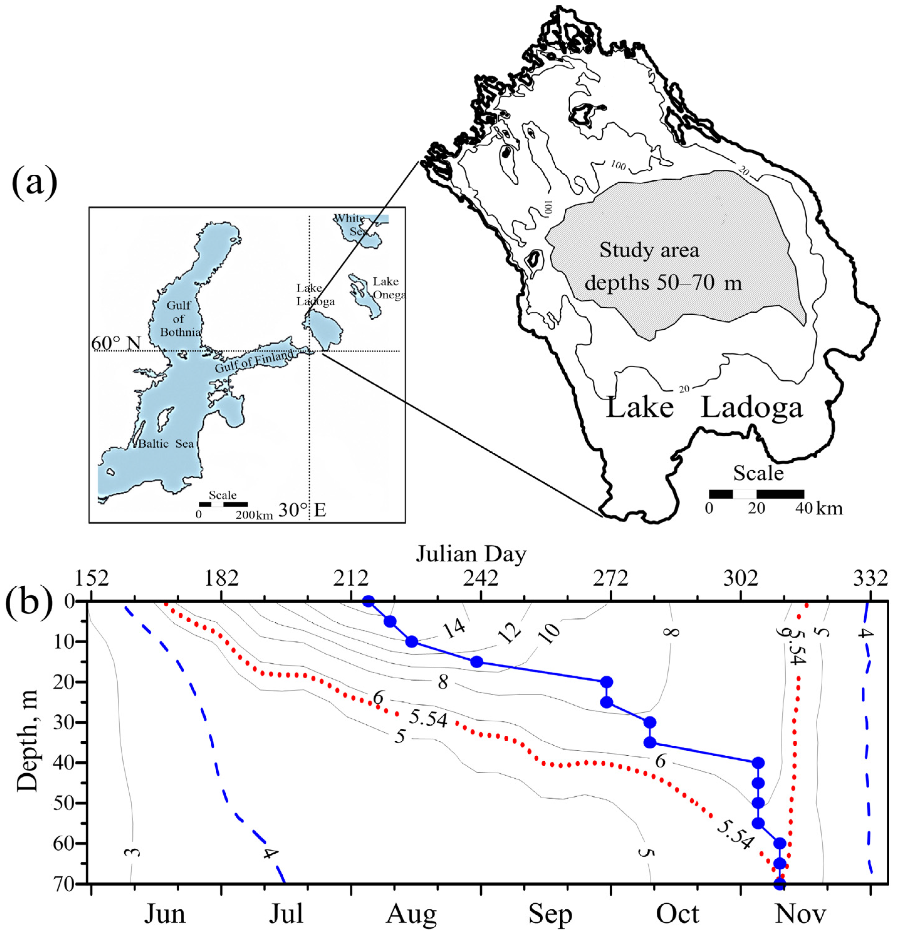
The largest dimictic lake in Europe, Lake Ladoga (Figure 1a) ranks 16th for area and 14th for volume among the 253 largest lakes in the world, with areas of more than 500 km2 [19]. The lake is an important link within the Volga River–Baltic–White Sea waterway system. The drainage area (258,000 km2) of Lake Ladoga extends over most of northwestern European Russia and eastern Finland. Deep freezing Lake Ladoga (water area 17,785 km2, average depth 48.3 m, maximum depth 230 m) is located in a temperate climatic zone (61° N, 32° E), which determines its ice regime and a well-defined annually repeating sequence of thermal structures during the year [4]. Ice phenomena on the surface of Lake Ladoga can be seen for more than half of the year (from the beginning of November to the middle of May). Ice cover lasts 172 ± 3 days in average. The mean residence time of the lake is about 12 years. A comprehensive limnological description of the lake can be found in [16].
Every year, in the dimictic Lake Ladoga, two complete mixings (overturns) of the water column occur: in autumn before the formation of ice, and in spring after the onset of ice melting, which is associated with an anomaly in fresh water density at a temperature of 3.98 °C [4]. These periods are characterized by intense free convection reaching the bottom (Figure 1b). After the overturn in spring, a stable density stratification forms in coastal areas (with temperatures above 4 °C) and a vernal thermal bar occurs [20]. In autumn, a similar situation takes place but in the reverse order; coastal regions have temperatures below 4 °C in contrast with central ones.
The mean annual air temperature for the period 1979–2018 is about 3.9 °C according to the weather station Sortavala, located in the north of the lake, with average annual amplitude of mean monthly temperatures of 25.5 °C. The average annual whole-lake (volume-weighted) temperature of Lake Ladoga is 3.8 °C, and the average annual temperature of the lake surface is 5.5 °C, with an average annual amplitude of water surface temperature of ~17 °C. The maximum surface temperature of the lake is reached in August.
The average temperature of the water mass of the lake is less than 4 °C for about 200 days of the year, and it exceeds this temperature for the remaining 165 days, reaching a maximum of 7.8 °C in the first week of September and the maximum heat content as well. The minimum temperature of the water mass (0.6 °C), as well as the lowest heat content, is observed in Lake Ladoga in the first week of April [21].
The annual amplitude of near-bottom water temperatures is not large and depends on the depth of the limnic zone of the lake. For depths more than 70 m, the temperature fluctuates throughout the year from 2 °C to 6 °C. These values are climatically significant physical parameters, important both for comparison with other dimictic lakes of the world, and for the analysis of climate changes and verification of thermohydrodynamic models.
2.2. Lake Ladoga Thermal Database
The earliest observations of open water temperature in Lake Ladoga were organized by Professor Juliy Schokalsky in 1897 and 1899 [22,23]. The Lake Ladoga thermal database (LLTD) provides lake-wide, in situ vertical water temperature profiles collected since 1897 to 2022 by research vessels of the Institute of Limnology of Russian Academy of Sciences, State Hydrometeorological Service, and other organizations. Collected using consistent methodology, the database includes the thermal water parameters with corresponding meteorological characteristics and lake depths as well [18]. The LLTD is the largest database among the databases on dimictic lakes in Russia. The overall number of source rows is ~300,000. The mean data density is about 350 measurements per km3. Therefore, the LLTD provides a useful basis for broad-scale inference for the investigation of spatial–temporal water surface, atmosphere thermal interaction, and thermal variations in Lake Ladoga as potentially affected by climate change. The Lake Ladoga computer thermal database has allowed the study of statistically significant changes in the spatial thermal structure of the lake. An extensive, comprehensive Atlas of Lake Ladoga [16] and a number of effective articles were prepared using the above database to update and refine thermic parameters of the lake.
2.3. Brief Thermal Structure of Central Part of Lake Ladoga
Quantitative estimates of the mean climatic course of the parameters of stable temperature stratification (including the thermocline layer) in Lake Ladoga are necessary to assess climatic variations relative to this course and their impact on the lake ecosystem. The mean annual surface temperature cycle is governed by exchanges of heat and depends on the depth distribution. It relates to the thermal bar evolution and the onset and duration of stable temperature stratification on a certain region of the lake [20]. We examine the central area of Lake Ladoga where the summer thermocline has largely the shape of a dome in most thermally stratified lakes [4]. The central part of Lake Ladoga has a rather flat bottom with depths in the range of 50–70 m. Stratification of the central area of Lake Ladoga occurs from mid-June. Recently, water temperatures and their main statistical characteristics on 8 horizons (0, 5, 10, 20, 30, 40, 50, and 100 m) were calculated for this limnetic region of Lake Ladoga from January to December [16]. The average period was 10 days, with shifting on 5 days that allowed the smoothing of high-frequency temperature fluctuations. The quantitative distribution of a seasonal course of the region-wide average vertical distribution of the water temperature for the central part of Lake Ladoga is shown on Figure 1b. Two periods (spring and autumn) of overturn (4 °C free convection) and the period of complete stable stratification with a well-defined thermocline from June to November are clearly visible.
Evidently, a ten-day average of water temperature at different horizons does not give an accurate quantitative description of the temperature regime of the selected area of the lake. However, analyses of water temperature variations and the depth of the upper quasi-homogeneous layer (epilimnion) (Figure 1b) indicate two features of the thermal regime of the central part of Lake Ladoga. Firstly, the deepening of the mixed layer (epilimnion) does not proceed linearly with time, accelerating in late autumn. Dots connected by solid lines indicate maximum water temperature on the horizons. This parameter characterizes the thickness of the epilimnion following the recommendations of James [24]. Secondly, the bottom temperature reaches its maximum in the annual cycle at the occurrence of fall overturning in early November, when the thickness of the mixed layer is comparable to the bottom depth. The dotted line depicts the change in the depth of the ~5.5 °C isotherm, corresponding to the maximum temperature near the bottom. In fact, Figure 1b shows the upper and lower boundary of the thermocline. These lines intersect at the date of the fall overturn or isothermia. Note that in lakes with shallow bottom depth, the autumn homogenous water temperature is higher than that of a deeper lake at the same latitude [25].
We will take into account these physical regularities of the dimictic Lake Ladoga later when creating the empirical relationships.
2.4. Determining of Stratification Parameters
In order to produce better estimates of the stratification parameters, we determine them from individual vertical water temperature profiles. Methodological approaches to the analysis of the variability of Lake Ladoga’s thermal structure are described in the paper [17]. Usually, during the summer stratification period, a vertical temperature structure is separated into three layers: epilimnion (surface mixed layer), metalimnion (thermocline), and hypolimnion (bottom layer). Seasonal thermocline in dimictic lakes is a region of strong vertical gradients of temperature located immediately below the surface mixed layer. It should be pointed out that metalimnion has a thickness which varies during stratification season. We suppose that a line of thermocline is the line of maximum gradient of water temperature or density. Above and below this line there are two parts which can be included in a common thermocline layer.
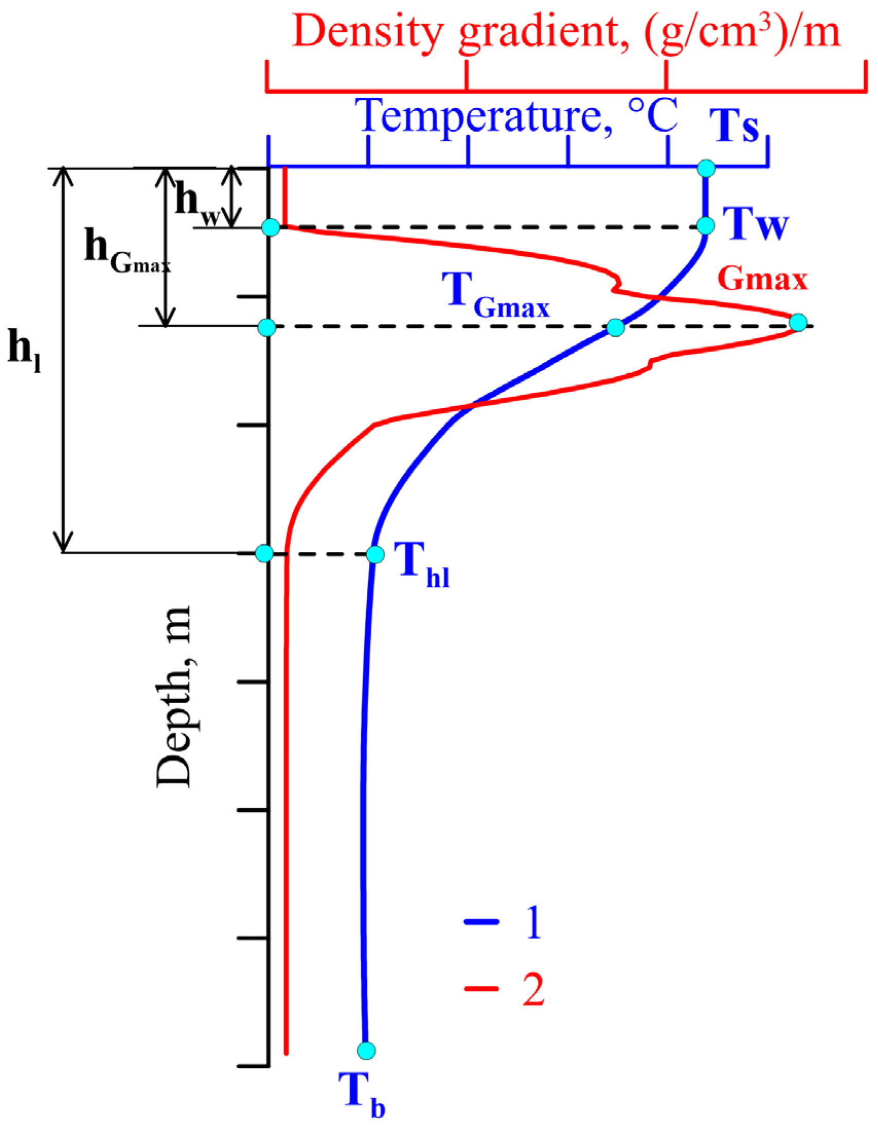
For a unified determination of the vertical temperature structure parameters in a large lake, it is necessary to create a methodology and software that allow the processing of large amounts of data on the vertical distribution of water temperature. The rLakeAnalyzer [26] is the most popular software for these purposes, which aims at calculating some thermal and energy characteristics of the lake based on long-term temperature measurements. We have expanded the set of parameters compared to this software. During the period of stable stratification, we characterize the vertical profile of water temperature following eight main parameters from surface to bottom H (Figure 2):
(1) Water surface temperature Ts (temperature of the upper mixed layer Tw differs from Ts no more than 0.5 °C);
(2) The thickness of the upper mixed layer (epilimnion) hw (upper boundary of the thermocline);
(3) The maximum value of the temperature (or density) gradient in the thermocline Gmax;
(4) The depth of the maximum value of the temperature (or density) gradient in the thermocline hGmax;
(5) Temperature at the depth of the maximum temperature (or density) gradient in the thermocline TGmax;
(6) Depth of the lower boundary of the thermocline (upper boundary of the hypolimnion layer) hl;
(7) Temperature at the lower boundary of the thermocline Thl;
(8) Temperature at the bottom Tb.
The epilimnion (i.e., mixed layer) is strictly valid only for homogenous fluids. After reviewing the techniques frequently employed to calculate epilimnion depth, Wilson et al. [27] came to the conclusion that there was no justified rationale for the choice of any certain technique. The method, which identifies the epilimnion depth as the shallowest depth at which the density is higher by 0.1 kg·m−3 than the surface density, has proven to be overall less dubious than other methods. Our choice is consistent with this proposal. To determine the depth of the epilimnion hw, we use the threshold value of water temperature difference between the surface and lower boundary of the epilimnion which is no more than 0.5 °C.
Notably, (Figure 2) the lower boundary of the epilimnion is the upper boundary of the thermocline layer. The actual exact concept of “a thermocline” refers to the surface of the maximum gradient of the temperature or density of water. The depth of the density gradient maximum hGmax is taken as the depth of the thermocline (Figure 2). We used the Chen–Millero formula for water density calculation [28]. The value of the vertical gradient of water density in the thermocline layer should be not less than 0.5 × 10⁻⁴ g/cm3/m [23]. Analogically, Toffolon et al. [29] assume 0.1 °C/m as a lower threshold for the existence of the thermocline.
The lower boundary of the thermocline layer hl is determined using the characteristic depth of the second derivative, the maximum curvature of the vertical temperature profile. The lower boundary of the metalimnion is the upper boundary of the hypolimnion, and the thickness of the thermocline layer is a = hl − hw. The difference between the station depth H and the lower boundary of the thermocline layer hl is the thickness of the hypolimnion.
The LLTD contains water temperature measurements, which were carried out at standard horizons, with varying accuracy, taken in the twentieth century with reversing thermometers, and in recent years with CTD probes. An important and necessary condition for finding the parameters of stable stratification is an equidistant distribution of water temperature (density) values on the studied vertical profile. Therefore, for each profile, we perform interpolation of temperature values with a discreteness of 0.5 m using the piecewise cubic Hermite polynomial. Since it does not give false maxima and inflection points, the smoothed data near local extrema look more correct [30]. After interpolation for each vertical water temperature profile, eight specified parameters are determined.
In order to calculate the average depths of occurrence of various elements of the vertical structure and to obtain a sufficiently reliable climatic seasonal course of the investigated characteristics, we used more than 10,000 surface-to-bottom water temperature profiles for the period of stable stratification from June to November from 1897 to the present.
Some difficulties were encountered in determining stratification parameters when anomalous data were detected, namely vertical water temperature profiles associated with short-period processes, both in the presence of a diurnal thermocline layer and in storms, upwelling, and frontal zones, which differ significantly from the vertical temperature profile in Figure 2 for each set of dates. Pursuing the task to calculate the climatic seasonal course of the selected characteristics, intensive work was carried out to identify these phenomena and exclude the discovered profiles from the analysis.
3. Results and Discussion
The suggested approach, which is based on the analyses of seasonal evolution of ensemble profiles of the Lake Ladoga central area, makes it possible to estimate all the necessary parameters and determine the mean climatic position of the thermocline layer from the onset of stable stratification to its dissipation.
3.1. Climatic Seasonal Course of Stratification Parameters
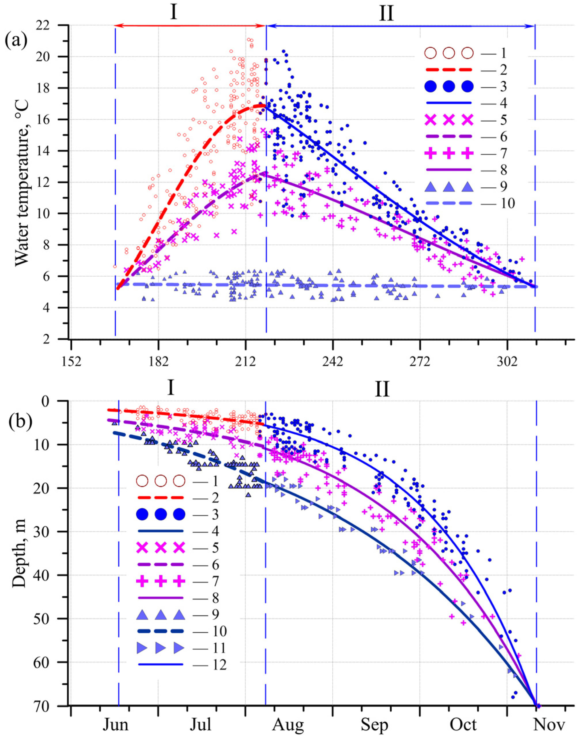
Vertical and temporal variations of Lake Ladoga temperature profiles are governed by exchanges of heat. Changes within the surface mixed layer depth are controlled by insolation and wind forcing during both heating and cooling periods. A typical hysteresis between the lake surface water temperature and air temperature can be noticeable, especially in deep lakes [31,32]. Graphs of the seasonal course of three significant parameters of Lake Ladoga’s vertical thermal structure are plotted from the onset of stable stratification to its dissipation (Figure 3a), namely observed water surface temperature Ts, observed temperature at the depth of the maximum density gradient in the thermocline TGmax, and observed temperature at the lower boundary of the thermocline Thl.
Evidently, seasonal courses of Ts and TGmax are not symmetric, unlike the first symmetric approximation used in the Fourier–Schmidt problem [8]. The heating period is shorter than the cooling period when stable stratification occurs. It is a general property of the thermal state of large dimictic lakes. The corresponding formulations for the seasonal course of water temperature are provided in articles [33,34,35].
We believe that it is very important to distinguish the period of heating from the period of cooling of water surface. Indeed, heating leads to the increased stability of temperature stratification and prevents the spread of heat inland. Cooling of the water surface causes free convection and enhances heat transfer to greater depths. Toffolon et al. [29] also propose to distinguish between the heating and cooling phases in the seasonal cycle of water surface temperature changes, achieved with computing dTs/dt.
The functional forms of temporal temperature cycle and the course of the thermocline boundaries deepening are useful for the examination and simulation of the vertical transport of heat from air to water. For each of the following time periods, the approximation curves were established: (I) prior to the date of the highest surface temperature within the area of interest; and (II) after that date, until complete vertical mixing takes place. The vertical line in Figure 3 depicts August 6 as the day of the climatic maximum of the water surface temperature in Lake Ladoga’s central region.
To describe the average climatic seasonal course of the surface temperature of the lake Ts (the upper quasi-homogeneous layer Tw) and the temperature at the depth of the maximum of the density gradient in the thermocline layer TGmax, we propose the following equation
where t = x/100, x-number of days from the beginning of the year.
During the period of stable stratification, the temperature of the lower boundary of the thermocline layer Thl or, equivalently, the temperature of the upper boundary of the hypolimnion, is approximately constant and equal to the yearly maximum near-bottom temperature in the selected region of the lake, when free convection reaches the bottom and the onset of turnover occurs in autumn. Thus, the temperatures are equal to each other (Ts = TGmax = Thl), which is in accordance with the earlier conclusion based on the ten-day time course of the water temperature in the central part of Lake Ladoga. As mentioned above, the curves intersect at only one point in autumn (Figure 3a).
For the time dependence of the change in the depth of the boundaries of the thermocline, the following function is chosen
Figure 3b represents three curves of deepening of the upper (hw), middle (hGmax), and lower (hl) boundaries of the thermocline. The behavior of the epilimnion differs during the heating period from that during the cooling period. Its depth does not change much until the maximum lake surface temperature is reached. During the cooling period, the depth of the epilimnion increases from 10 m to the bottom depth within two months. The variations are in agreement with the conclusions drawn from the ten-day average and the developed approximation curves. The curves intersect at the same point (bottom depth H) during the autumn overturn (hw = hGmax = hl = H), which is physically justified.
Each approximation curve is calculated for both heating and cooling periods. The nonparametric Mann–Kendall test shows the significance of trends (α = 0.05). Determination coefficients for the heating period (0.33–0.68) are less than those for the cooling period (0.76–0.98). This is due to the irregular wind influence on the epilimnion temperature Tw during the heating period, whereas in the cooling period, the main role belongs to the constantly existing convective mixing. The empirical coefficients a1, d, c, a2, r for regression dependencies (1) and (2) are provided in [17].
3.2. The Rate of Change in Water Temperature and the Depth of the Thermocline Boundaries
Much less documented compared to a surface case are the trends in temperature regime of the lake’s mid-level and bottom water. To fill them up, we differentiate the analytic expressions (1) and (2), and determine the time dependencies for the climatic rates of change in water temperature (dTs/dt) and thermocline depth (dh/dt) in the central region of Lake Ladoga.
The highest rate of water temperature change at the heating stage takes place in late June–early July, which at the water surface, is 0.32 °C/day, while in the thermocline layer, it is 0.18 °C/day. The peak velocity during the cooling stage at the surface occurs in late August–early September and is 0.14 °C/day, whereas in the thermocline, it is 0.08 °C/day and takes place between September and early October. Both rates of change for the surface and the thermocline temperatures tend to zero during the autumn overturn [36]. In the fall, in the last stage of sustained surface cooling in the thermocline, temperature profiles become quasi-uniform because the thermocline has been weakened and deepened and finally reaches the bottom. At this date the epilimnion thickness is equal to the bottom depth [37], and the bottom temperature hits its maximum during the annual cycle [17].
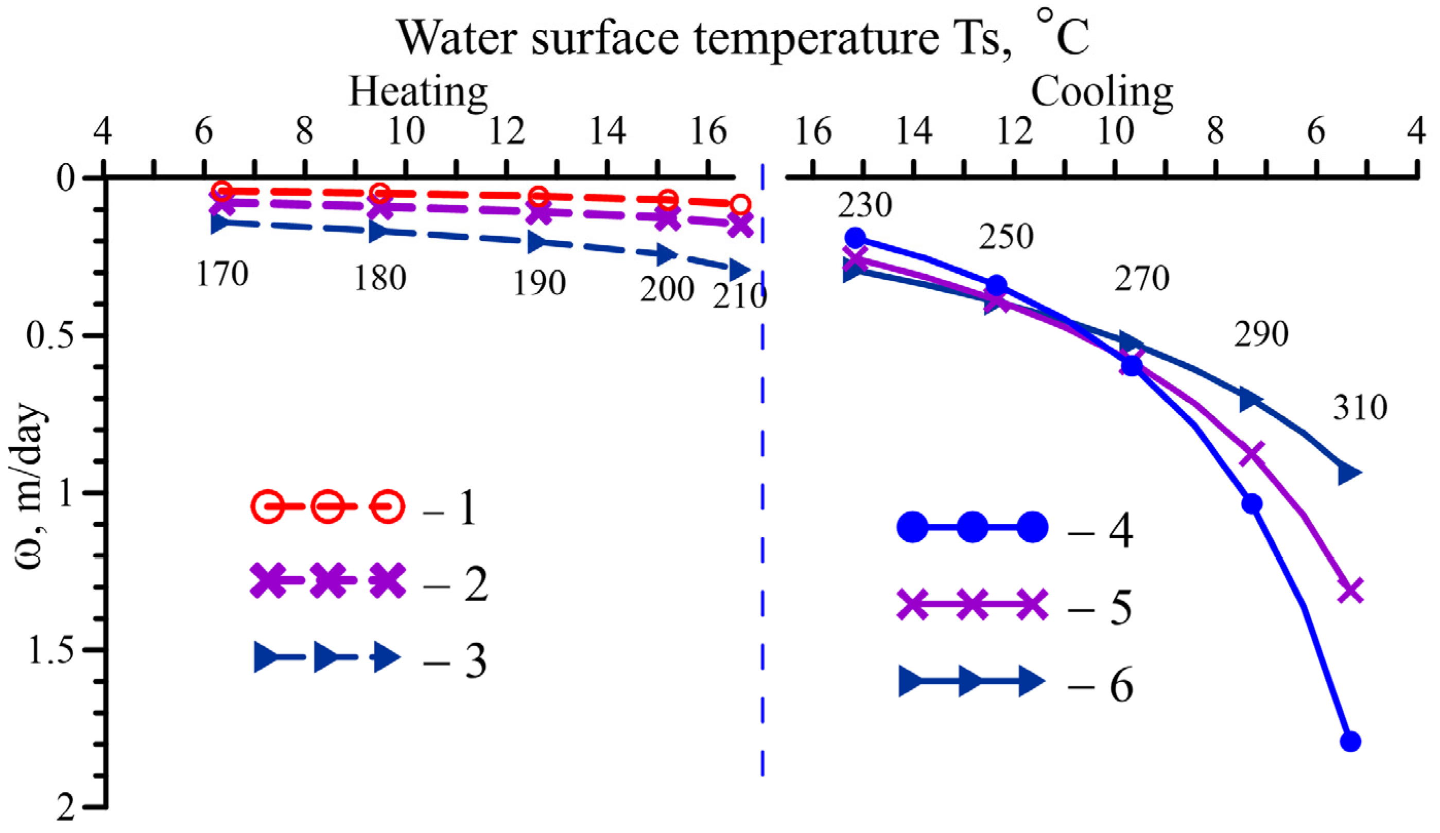
Figure 4 shows the variations in thermocline boundary depth depending on surface water temperature for two different periods.
To estimate the deepening parameters of the thermocline layer, we estimated at first the deepening rates of the three surfaces hw, hGmax, and hl, which increase over time and reach their maxima during the stage of complete autumn mixing (Figure 4).
During the period of heating, they do not fluctuate very much, only within the range 0.1–0.3 m/day. During the cooling period, under the influence of free convection, rates increase drastically. The maximum rates of hw deepening during the period of full autumn mixing reach 1.8 m/day, and the lower boundary of the thermocline hl reaches 0.95 m/day. This is consistent with the conclusions drawn on the long-term temperature measurements of the near-bottom water in the dimitic Lake Michigan [38].
Starting from the end of September (270 days), the sinking rates of the three thermocline boundaries begin to differ at a surface temperature of Ts = 10 °C. This is the period during which the thickness of the thermocline reaches its maximum (Figure 5). This temperature is an indicator of changes in vertical heat exchange, which can be recorded using remote sensing methods.
3.3. Temporal Course of Maximum Vertical Temperature (Density) Gradients and Thickness of Various Layers
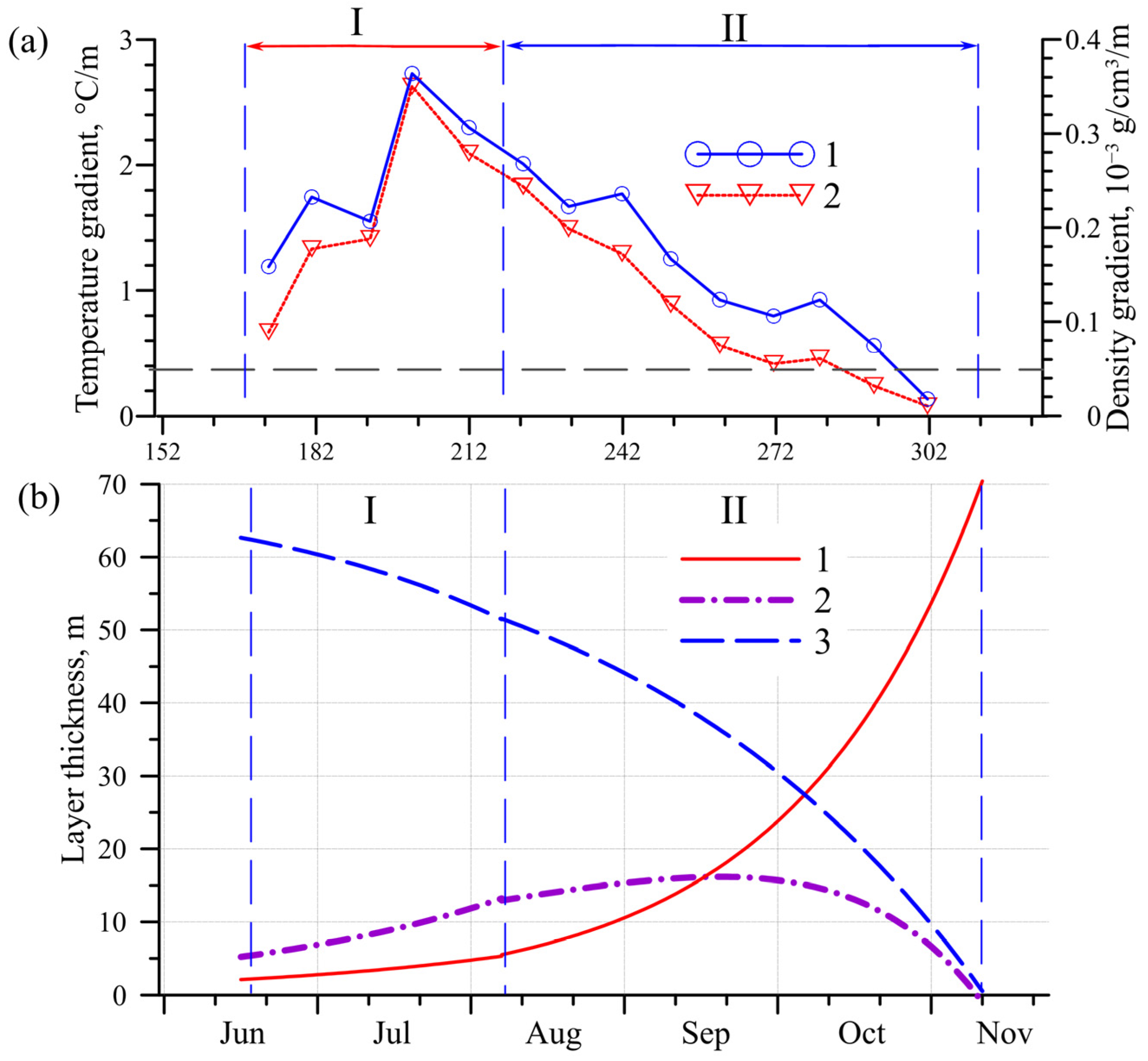
Depending on the strength of the vertical mixing, solar insolation, and water transparency, the depth and shape of the thermocline vary with season and local environmental conditions. The main seasonal cycles (10 day averaging) of maximum temperature gradients and water density gradients in thermocline are shown in Figure 5a.
The highest vertical density (temperature) gradients of ~0.4 × 10⁻³ g/cm3/m (with a vertical gradient of water temperature of ~2.5 °C/m) at a depth of ~10 m are observed prior to establishing the maximum surface water temperature. At that time, the mixed layer is 3–4 m thick. The density criterion for the thermocline, provided in [23], is depicted by the dashed line in Figure 5a. At the time of full autumn mixing, during the cooling phase, the gradients drop to almost zero values. It should be pointed out that the vertical gradients of temperature and density on certain dates may exceed the values obtained with the 10 day average by several times.
To our knowledge, the estimations of thicknesses of epilimnion, metalimnion, and hypolimnion, based on the empirical Formula (2), are obtained for the first time, making it possible to visualize their temporal course for the period of stable stratification (Figure 5b). According to K. Rodgers [37], the hypolimnion occupies the entire water column from the surface to the bottom after the passage of the thermobar at a certain height. The epilimnion thickness does not change considerably throughout the heating phase. Both the thicknesses of the upper mixed layer (epilimnion) and the metalimnion layer significantly increase at the onset of the cooling phase, brought on by free convection (Figure 5b). The thicknesses of the epilimnion and metalimnion layers are comparable and are 16.2 m at the depth of the maximum density gradient of ~25 m during the period of maximum heat content of the lake in the second half of September. At this time, the thermocline layer maximum thickness is 23% of the bottom depth.
4. Conclusions
For the first time for Lake Ladoga, the complete cycle of the development, growth, and destruction of the summer–autumn thermocline from early spring to late fall is well described with empirical relationships based on the physical features governing the water temperature variations. It should be kept in mind that we study the climatic seasonal course of thermic characteristics of the central area of Lake Ladoga. Our analysis disregards vertical profiles of water temperature taken in the presence of a daily thermocline layer, as well as during storms, upwellings, and frontal zones, which deviate substantially from the lake’s three-layer structure.
Our results show that the developed simplification and generalization of the parameters of stable thermal stratification quantitatively describe the mean changes of water temperature and the depth of stratification parameters in the period from June to November for the central part of Lake Ladoga. The proposed regression dependencies have the same analytical forms for both the underlying and overlying layers. Analytical forms vary in empirical coefficients, which emphasize their differences but allow comparison with each other.
The quantitative assessments of the evolution of seasonal stratification in Lake Ladoga have been described, and these results can serve as a basis for verification and improvement of the various thermal models. Moreover, the proposed approximation forms can be tested on other large dimictic lakes, such as Lake Ontario [9], Lake Eri [39], and Lake Superior [40].
Computed values of the lake’s stable stratification are actually climatic norms against which it is necessary to assess climate change. The shift in the thermal regime of Lake Ladoga will have a profound impact on the ecosystem of the largest European lake. In fact, the degree of convection and thermocline depth may structure the planktonic communities [41,42], as plankton rely on vertical circulation to remain in the photic zone [43].
Author Contributions
Conceptualization, M.N.; methodology M.N. and V.G.; investigation, M.N. and V.G.; writing—original draft preparation, M.N. and V.G.; writing—review and editing, M.N and V.G. All authors have read and agreed to the published version of the manuscript.
Funding
The work was supported by State Task no. 0154-2019-0001 “Comprehensive Assessment of the Dynamics of Ecosystems of Lake Ladoga and Water Bodies of Its Basin under the Influence of Natural and Anthropogenic Factors”.
Data Availability Statement
Primary data from Lake Ladoga (in situ water temperature measurements at hydrological and meteorological stations from research vessels) are unavailable for downloading in accordance with the policy of Hydrometeorological Service of Russian Federation and Institute of Limnology of the Russian Academy of Sciences, Federal Research Center of the Russian Academy of Sciences (SPC RAS).
Acknowledgments
We are most grateful for two anonymous referees for useful comments.
Conflicts of Interest
The authors declare that they have no conflict of interest.
References
- Adrian, R.; O’Reilly, C.M.; Zagarese, H.; Baines, S.B.; Hessen, D.O.; Keller, W.; Livingstone, D.M.; Sommaruga, R.; Straile, D.; Donk, E.V.; et al. Lakes as sentinels of climate change. Limnol. Oceanogr. 2009, 54, 2283–2297. [Google Scholar] [CrossRef] [PubMed]
- O’Reilly, C.M.; Sharma, S.; Gray, D.K.; Hampton, S.E.; Read, J.S.; Rowley, R.J.; Schneider, P.; Lenters, J.D.; McIntyre, P.B.; Kraemer, B.M.; et al. Rapid and highly variable warming of lake surface waters around the globe. Geophys. Res. Lett. 2015, 42, 1773–10781. [Google Scholar] [CrossRef]
- Boyarinov, P.M.; Petrov, M.P. Processy Formirovaniya Termicheskogo Rezhima Glubokih Presnovodnyh Vodoyomov (Processes of the Formation of Thermal Regime of Deep Freshwater Reservoirs); Nauka: Leningrad, Russia, 1991; 178p. (In Russian) [Google Scholar]
- Tikhomirov, A.I. Termika Krupnyh Ozyor (The Thermal Regime of Large Lakes); Nauka: Leningrad, Russia, 1982; 232p. (In Russian) [Google Scholar]
- Hutchinson, G.E. A Treatise on Limnology. V.1. Geography and Physics of Lakes; Wiley-Interscience: New York, NY, USA, 1957; 1015p. [Google Scholar]
- Carpenter, S.R.; Fisher, S.G.; Grimm, N.B.; Kitchell, J.F. Global change and fresh-water ecosystems. Annu. Rev. Ecol. Syst. 1992, 23, 119–139. [Google Scholar] [CrossRef]
- King, J.; Shuter, B.; Zimmerman, A. The response of the thermal stratification of South Bay (Lake Huron) to climatic variability. Can. J. Fish. Aquat. Sci. 1997, 54, 1873–1882. [Google Scholar] [CrossRef]
- Sundaram, T.R.; Rehm, R.G. The seasonal thermal structure of deep temperate lakes. Tellus 1973, 25, 157–167. [Google Scholar] [CrossRef]
- McCormik, M.J.; Scavia, D. Calculation of Vertical Profiles of Lake-Averaged Temperature and Diffusivity in Lakes Ontario and Washington. Water Resour. Res. 1981, 17, 305–310. [Google Scholar] [CrossRef]
- Fang, X.; Stefan, H.G. Long-term lake water temperature and ice cover simulations/measurements. Cold Reg. Sci. Technol. 1996, 24, 289–304. [Google Scholar] [CrossRef]
- Kirillin, G.; Hochschild, J.; Mironov, D.; Terzhevik, A.; Golosov, S.; Nützmann, G. FLake-Global: Online lake model with worldwide coverage. Environ. Model. Softw. 2011, 26, 683–684. [Google Scholar] [CrossRef]
- Golosov, S.; Mironov, D. Temperature model for Lake Ladoga (TEMIX)–Institute of Limnology. Hydrological monitoring and modelling of Lake Ladoga with recommendation for the further research. Kerelian Inst. Univ. Joensuu 2000, 2, 52–54. [Google Scholar]
- Filatov, N.N. (Ed.) Diagnosis and Forecast of Thermohydrodynamics and Ecosystems of the Great Lakes of Russia; KarRC RAS: Petrozavodsk, Russia, 2020; 255p. (In Russian) [Google Scholar]
- Stepanenko, V.; Mammarella, I.; Ojala, A.; Miettinen, H.; Lykosov, V.; Vesala, T. LAKE 2.0: A model for temperature, methane, carbon dioxide and oxygen dynamics in lakes. Geosci. Model Dev. 2016, 9, 1977–2006. [Google Scholar] [CrossRef]
- Jorgensen, S.E. A review of recent developments in lake modeling. Ecol. Modell. 1994, 221, 689–692. [Google Scholar] [CrossRef]
- Rumyantsev, V.A. (Ed.) Ladozhskoe Ozero I Dostoprimechatel’nosti Ego Poberezh’ya (Lake Ladoga and Sights of Its Coast): Atlas; Nestor-History: St. Petersburg, Russia, 2015; 200p. (In Russian) [Google Scholar]
- Naumenko, M.A.; Guzivaty, V.V. Methodological Approaches and Results of an Analysis of the Climatic Seasonal Course of Stable Stratification Parameters of a Dimictic Lake (Case Study of the Central Part of Lake Ladoga). Izv. Atmos. Ocean. Phys. 2022, 58, 44–53. [Google Scholar] [CrossRef]
- Guzivaty, V.V.; Karetnikov, S.G.; Naumenko, M.A. Opyt sozdaniya i ispol’zovaniya banka termicheskih dannyh Ladozhskogo ozera (Experience of the creation and use of the thermal databank for Lake Ladoga). Geogr. Prir. Resur. 1998, 3, 89–96. (In Russian) [Google Scholar]
- Tilzer, M.M.; Serruya, C. (Eds.) Large Lakes. Ecological Structure and Function; Springer: Berlin/Heidelberg, Germany, 1990; 692p. [Google Scholar]
- Naumenko, M.A. Peculiarities of the climatic correlation of the temperature of the water surface and the driving air layer during the spring warming of Lake Ladoga. Fundam. Prikl. Gidrofiz. 2021, 14, 78–88. [Google Scholar]
- Naumenko, M.A.; Karetnikov, S.G.; Guzivaty, V.V. Thermal regime of Lake Ladoga as a typical dimictic lake. Limnol. Rev. 2007, 7, 63–70. [Google Scholar]
- Schokalsky, J. Lake Ladoga from a thermic point of view. Weather Rev. 1901, 29, 63–64. [Google Scholar] [CrossRef]
- Molchanov, I.V. Ladozhskoe Ozero (Lake Ladoga); Gidrometeoizdat: Moscow, Russia; Leningrad, Russia, 1945; 557p. (In Russian) [Google Scholar]
- James, R. Ocean Thermal Structure Forecasting; U.S. Naval Oceanographic Office: Washington, DC, USA, 1966; 217p. [Google Scholar]
- Skowron, R. Letnia Stratyfikacja Termiczna Wody w Jeziorach na Niżu Polskim (The Summer Thermal Stratification of Water in the Lakes in the Polish Lowlands); Wydawnictwo Naukowe Uniwersytetu Mikolaja Kopernika: Toruń, Poland, 2022; 336p, ISBN 978-83-231-5058-9. [Google Scholar]
- Read, J.; Hamilton, D.; Jones, I.; Muraoka, K.; Winslow, L.; Kroiss, R.; Wu, C.; Gaiser, E. Derivation of lake mixing and stratification indices from high-resolution lake buoy data. Environ. Model. Softw. 2011, 26, 1325–1336. [Google Scholar] [CrossRef]
- Wilson, H.L.; Ayala, A.I.; Jones, I.D.; Rolston, A.; Pierson, D.; de Eyto, E.; Grossart, H.-P.; Perga, M.-E.; Woolway, R.I.; Jennings, E. Variability in epilimnion depth estimations in lakes. Hydrol. Earth Syst. Sci. 2020, 24, 5559–5577. [Google Scholar] [CrossRef]
- Chen, C.; Millero, F. Precise thermodynamic properties for natural waters covering only the limnological range. Limnol. Oceanogr. 1986, 31, 657–662. [Google Scholar] [CrossRef]
- Toffolon, M.; Yousefi, A.; Piccolroaz, S. Estimation of the thermally reactive layer in lakes based on surface water temperature. Water Resour. Res. 2022, 58, e2021WR031755. [Google Scholar] [CrossRef]
- Stepanov, M.E. Nekotorye voprosy, svyazannye s interpolyacionnym mnogochlenom Ermita (Some issues related to the Hermite interpolation polynomial). Model. Anal. Dannykh 2014, 1, 139–161. [Google Scholar]
- Toffolon, M.; Piccolroaz, S.; Majone, B.; Soja, A.-M.; Peeters, F.; Schmid, M.; Wüest, A. Prediction of surface temperature in lakes with different morphology using air temperature. Limnol. Oceanogr. 2014, 59, 2185–2202. [Google Scholar] [CrossRef]
- Naumenko, M.A.; Guzivaty, V.V. Climatic relationships between air temperature and water temperatures in different limnic areas of lake Ladoga. Geogr. Prir. Resur. 2022, 1, 83–92. (In Russian) [Google Scholar] [CrossRef]
- Lesht, B.M.; Brandner, D.J. Functional representation of Great Lakes surface temperatures. J. Great Lakes Res. 1992, 18, 98–107. [Google Scholar] [CrossRef]
- Naumenko, M.A.; Karetnikov, S.G. Seasonal evolution of the spatial distribution of water surface temperature in Lake Ladoga related to its morphometry. Dokl. Earth Sci. 2002, 386, 818–820. [Google Scholar]
- Palshin, N.I.; Efremova, T.V. Stohasticheskaya model’ godovogo hoda temperatury poverhnosti vody v ozerah (Stochastic model of annual variations of water surface temperature in lakes). Meteorol. Hydrol. 2005, 3, 85–94. (In Russian) [Google Scholar]
- Anderson, E.J.; Stow, C.A.; Gronewold, A.D.; Mason, L.A.; McCormick, M.J.; Qian, S.S.; Ruberg, S.A.; Beadle, K.; Constant, S.A.; Hawley, N. Seasonal overturn and stratification changes drive deepwater warming in one of Earth’s largest lakes. Nat. Commun. 2021, 12, 1688. [Google Scholar] [CrossRef]
- Rodgers, G.K. A note on thermocline development and the thermal bar in Lake Ontario. In Symposium of Garda, Hydrology of Lakes and Reservoirs; Proceedings of the International Association of Scientific Hydrology; IAHS Press: Wallingford, UK, 1965; Volume 70, pp. 401–405. [Google Scholar]
- Fichot, C.; Matsumoto, K.; Holt, B.; Gierach, M.; Tokos, K. Assessing change in the overturning behavior of the Laurentian Great Lakes using remotely sensed lake surface water temperatures. Remote Sens. Environ. 2019, 235, 111427. [Google Scholar] [CrossRef]
- Beletsky, D.; Hawley, N.; Rao, Y.R.; Vanderploeg, H.A.; Beletsky, R.; Schwab, D.J.; Ruberg, S.A. Summer thermal structure and anticyclonic circulation of Lake Erie. Geophys. Res. Lett. 2012, 39, L06605. [Google Scholar] [CrossRef]
- Titze, D.J.; Austin, J.A. Winter thermal structure of Lake Superior. Limnol. Oceanogr. 2014, 59, 1336–1348. [Google Scholar] [CrossRef]
- Bouffard, D.; Zdorovennova, G.; Bogdanov, S.; Efremova, T.; Lavanchy, S.; Palshin, N.; Zdorovennov, R. Under-ice convection dynamics in a boreal lake. Inland Waters 2019, 9, 142–161. [Google Scholar] [CrossRef]
- Kelley, D.E. Convection in ice-covered lakes: Effects on algal suspension. J. Plankton Res. 1997, 19, 1859–1880. [Google Scholar] [CrossRef]
- Yang, B.; Wells, M.G.; Li, J.; Young, J. Mixing, stratification, and plankton under lake-ice during winter in a large lake: Implications for spring dissolved oxygen levels. Limnol. Oceanogr. 2020, 65, 2713–2729. [Google Scholar] [CrossRef]
Figure 1.
Location of Lake Ladoga (a) and average water temperature distribution for the stratification period in central part of the lake (b).
Figure 1.
Location of Lake Ladoga (a) and average water temperature distribution for the stratification period in central part of the lake (b).

Figure 2.
Scheme for determining the thermocline parameters based on the vertical profile of the water temperature. See text for notation. 1—temperature, °C, 2—density gradient, (g/cm3)/m.
Figure 2.
Scheme for determining the thermocline parameters based on the vertical profile of the water temperature. See text for notation. 1—temperature, °C, 2—density gradient, (g/cm3)/m.

Figure 3.
Seasonal variation of stable stratification parameters for periods of heating (I) and cooling (II). (a) Symbols represent the observed water temperature Ts (1,3), TGmax (5,7), and Thl (9) for each period, respectively. Lines represent approximation curves according to Formula (1) for Ts (2,4), TGmax (6,8), and Thl (10). (b) Symbols represent the observed depth hw (1,3), hGmax (5,7), and hl (9,11) for each period, respectively. Lines represent approximation curves according to Formula (2) for hw (2,4), hGmax (6,8), and hl (10,12).

Figure 4.
Deepening rate ω (m/day) of the upper boundary of the thermocline hw (1), the depth of the maximum water density gradient hGmax (2), the lower boundary of the thermocline hl (3) for the heating period and the cooling period (4), (5), (6), respectively, depending on the surface temperature Ts. Numbers near symbols are the days from the beginning of the year.

Figure 5.
Seasonal variation of (a) maximum temperature (1) and water density (2) gradients; (b) thickness of the epilimnion (mixed layer) (1), thickness of the thermocline (2), and thickness of the hypolimnion (3) for the period of heating (I) and cooling (II) of the surface of Lake Ladoga. The horizontal dashed line depicts the thermocline density criterion [23].

Disclaimer/Publisher’s Note: The statements, opinions and data contained in all publications are solely those of the individual author(s) and contributor(s) and not of MDPI and/or the editor(s). MDPI and/or the editor(s) disclaim responsibility for any injury to people or property resulting from any ideas, methods, instructions or products referred to in the content. |
© 2023 by the authors. Licensee MDPI, Basel, Switzerland. This article is an open access article distributed under the terms and conditions of the Creative Commons Attribution (CC BY) license (https://creativecommons.org/licenses/by/4.0/).
Share and Cite
MDPI and ACS Style
Naumenko, M.; Guzivaty, V. Seasonal Evolution of Stable Thermal Stratification in Central Area of Lake Ladoga. Limnol. Rev. 2023, 23, 177-189. https://doi.org/10.3390/limnolrev23030011
AMA Style
Naumenko M, Guzivaty V. Seasonal Evolution of Stable Thermal Stratification in Central Area of Lake Ladoga. Limnological Review. 2023; 23(3):177-189. https://doi.org/10.3390/limnolrev23030011
Chicago/Turabian StyleNaumenko, Mikhail, and Vadim Guzivaty. 2023. "Seasonal Evolution of Stable Thermal Stratification in Central Area of Lake Ladoga" Limnological Review 23, no. 3: 177-189. https://doi.org/10.3390/limnolrev23030011