Understanding the Importance of Dynamic Landscape Connectivity
by
 , ,
, ,
Katherine A. Zeller
1,* ,
,
Rebecca Lewison
2,
Robert J. Fletcher
3,
Mirela G. Tulbure
4 and
Megan K. Jennings
2 1
Aldo Leopold Wilderness Research Institute, Rocky Mountain Research Station, United States Forest Service, 790 East Beckwith Ave, Missoula, MT 59801, USA
2
Department of Biology, San Diego State University, San Diego, CA 92182, USA
3
Department of Wildlife Ecology and Conservation, University of Florida, Gainesville, FL 32611, USA
4
Center for Geospatial Analytics, North Carolina State University, Raleigh, NC 27695, USA
*
Author to whom correspondence should be addressed.
Land 2020, 9(9), 303; https://doi.org/10.3390/land9090303
Submission received: 31 July 2020
/
Revised: 24 August 2020
/
Accepted: 27 August 2020
/
Published: 29 August 2020
(This article belongs to the Special Issue Dynamic Landscape Connectivity)
Abstract
:Landscape connectivity is increasingly promoted as a conservation tool to combat the negative effects of habitat loss, fragmentation, and climate change. Given its importance as a key conservation strategy, connectivity science is a rapidly growing discipline. However, most landscape connectivity models consider connectivity for only a single snapshot in time, despite the widespread recognition that landscapes and ecological processes are dynamic. In this paper, we discuss the emergence of dynamic connectivity and the importance of including dynamism in connectivity models and assessments. We outline dynamic processes for both structural and functional connectivity at multiple spatiotemporal scales and provide examples of modeling approaches at each of these scales. We highlight the unique challenges that accompany the adoption of dynamic connectivity for conservation management and planning in the context of traditional conservation prioritization approaches. With the increased availability of time series and species movement data, computational capacity, and an expanding number of empirical examples in the literature, incorporating dynamic processes into connectivity models is more feasible than ever. Here, we articulate how dynamism is an intrinsic component of connectivity and integral to the future of connectivity science.
1. Introduction
Protected areas comprise less than 15% of the terrestrial area of the planet [1], and the remaining unprotected natural lands are becoming increasingly threatened due to deforestation and the expansion of urban areas and agricultural land [2,3]. Habitat loss and fragmentation are key drivers of biodiversity loss [4,5], and can increase the risk of extinction for species [6,7]. Identifying, maintaining, and enhancing landscape connectivity—the degree to which the landscape facilitates movement—is considered an important conservation tool that can reduce the negative effects of habitat loss and fragmentation [7,8,9,10,11]. Connectivity has been shown to increase the movement of individuals, which contributes to dispersal, migration, and gene flow and promotes population recolonization or establishment in unoccupied areas [12,13]. Connectivity also maintains viable metapopulations and can contribute to the demographic rescue of small, isolated populations [2,14].
Because of the positive effects of connected landscapes [11], connectivity research has quickly grown, reflected in the almost doubling per decade of connectivity conservation plans [15]. Connectivity research emerged from the marriage of classic metapopulation theory [16,17] and landscape ecology [18,19,20]. Metapopulation theory highlighted the importance of landscape structure and dispersal in population viability, and eventually evolved into spatially realistic metapopulation models [21]. These models formally incorporated connectivity and its importance in patch colonization and metapopulation persistence metrics; however, connectivity was conceptualized only as straight-line distance [22]. Landscape ecology, inspired by Merriam’s first definition of “landscape connectivity” [23], highlighted the fact that movement among colonized patches is not only a function of distance, but also of the quality of the matrix (the portion of the landscape that extends among identified habitat patches) in facilitating movement [24,25]. Connectivity analyses typically explore patch, corridor, and matrix parameters in terms of how these components of the landscape may promote or limit movement across the landscape [26].
As landscape ecology has evolved and developed, the recognition of landscapes as dynamic has become the norm (e.g., dynamic surface water bodies, phenology, forests that undergo clear-cuts, disturbances). However, despite this conceptual evolution and the established theoretical and conceptual understanding of metapopulation dynamics [27], landscape connectivity approaches usually lack the quantification of dynamics over seasonal, yearly, and decadal scales. Because landscapes are continually changing across scales, connectivity for a single instance may not apply universally across time (e.g., Figure 1); therefore, incorporating dynamics into connectivity modeling has the potential to result in a more realistic and accurate understanding of connectivity.
Like static connectivity models, dynamic connectivity models can be divided into two broad approaches (see Box 1): (1) structural connectivity, where the focus is on the contiguity of landscape features (e.g., forest strips along riparian areas, hedgerows), under the assumption that configuration will facilitate movement or flow; or (2) functional connectivity, where the focus is not only on landscape features, but also on species-specific responses to those landscape features [18]. Changes in structural connectivity are more easily observed and quantified than changes in functional connectivity, which are context-specific and affected by landscape change as well as population density, season, life stage, food availability, vagility, and perceptual range. Whether modeling structural or functional connectivity, the importance of considering dynamism cannot be understated: static connectivity models can underestimate connectivity, bias connectivity metrics, and result in different conservation priorities when compared with dynamic models [28,29,30].
Limits on data availability and computational power have likely hindered modeling the complexities of connectivity in dynamic systems. However, with the release of large troughs of decades of time-series satellite data, the availability of future climate and land-use projections, the increased ability to track species’ movements, and advances in computational capacity which can support the systematic modelling of landscape dynamics, dynamic connectivity analyses are on the rise. The challenge then becomes how much and to what extent dynamism should be incorporated into a connectivity model, and how to meaningfully distill the results of these dynamic complexities so that they can be used in conservation planning. The familiar concepts of spatial prioritization such as complementarity, redundancy, and irreplaceability (see Box 1), widely applied to conservation planning in static environments [31], can also provide a foundation for dynamic connectivity planning. Building on such a foundation by incorporating dynamic processes into conservation planning provides an opportunity to develop more realistic landscape representations and strengthen conservation outcomes.
In this paper, we aim to contextualize the emergence and importance of dynamic connectivity. We provide an overview of the rise of dynamic connectivity and explain the importance of including dynamism in connectivity models. Building on this conceptual foundation, we identify aspects of dynamic connectivity at different spatiotemporal scales, highlight approaches for connectivity analyses in a dynamic framework, and discuss how dynamic connectivity can support effective landscape management and conservation.
Box 1. Glossary of key terms for dynamic landscape connectivity. Some of these terms, such as complementarity, irreplaceability, and redundancy, are an extension and new application of the same terms used in the literature for conservation prioritization.

2. Moving from Static to Dynamic Landscapes
Whereas landscapes were traditionally considered to be static in early modeling and planning efforts, the dynamic nature of landscapes is now well established and embraced [32]. Water bodies, ocean areas, forests, grasslands, shrublands, and other systems are all recognized as dynamic systems that undergo change from natural and anthropogenic disturbances and other ecosystem processes. Despite the acceptance of landscapes (and seascapes) as dynamic, current paradigms and approaches to landscape connectivity are usually evaluated using static, single spatial “snapshots” in time [33,34] or seasonal time periods [35,36,37]. Ignoring dynamics in landscapes that have high natural temporal variability in available habitat, quality, and spatial arrangement can lead to erroneous conclusions regarding connectivity. For example, Bishop-Taylor et al. [30] evaluated static and dynamic connectivity to prioritize habitats for conservation. They found that for regions that exhibit a high spatiotemporal variability, static connectivity did not effectively quantify connectivity [30]. In addition, Wimberly et al. [38] observed differences in population sizes and patch occupancy between models that used static versus dynamic landscapes. What these and other examples (e.g., [39,40,41]) demonstrate is that quantifying landscape connectivity in a dynamic framework allows for the identification of both dynamic and persistent areas for spatiotemporal connectivity. Despite these examples, there is a recognized knowledge gap in conceptual and applied approaches to address dynamic landscape connectivity [42].
In contrast to connectivity work in terrestrial systems, the concept of connectivity as a dynamic process has been central to understanding how species, populations, and communities respond to and interact with dynamic environments in ocean and freshwater research [43,44]. Dynamic connectivity is recognized to be a primary driver of population dynamics in these systems, integral to reproduction, recruitment, dispersal, and survival. In oceans, the concept of dynamic connectivity first centered largely on larval transport and settlement. While early studies considered connectivity to be stable or invariant, for the past several decades connectivity has been recognized as an emergent property, reflecting underlying dynamic processes [45] and a coupled relationship between organisms and the biophysical ocean environment [46]. The integrated exploration of biophysical modelling and connectivity within ocean science may explain why dynamic connectivity is foundational to population dynamics research both in real time and for future projections or forecasts of the potential impacts of shifts in connectivity [47]. The concept of dynamic connectivity is also central to ocean resource management, where research on marine protected areas has found that patterns of connectivity, which change across short temporal and large spatial scales, are critical to maintaining viable ecosystems and populations [48,49,50].
Similarly, the importance of incorporating connectivity as a dynamic feature has been identified in freshwater research [51,52], with analyses of longitudinal data suggesting that static approaches to assess connectivity fail to capture key connectivity measures [30]. Given the dynamic processes that govern many aquatic systems—e.g., droughts, floods, intermittent flow—it is not surprising that connectivity metrics have been found to shift by orders of magnitude in response to changing conditions [53]. In wetlands, connectivity across the landscape has also been found to be an emergent and dynamic property [54] and closely tied to climate-driven variation and climate change [55]. These dynamic connectivity examples in marine and aquatic systems highlight the potential importance of incorporating dynamics into landscape connectivity and serve as guideposts for how dynamism has been integrated in other systems.
3. Key Features of Dynamic Landscape Connectivity
The key features of dynamic landscape connectivity involve the interplay of changes in the landscape and changes in movement and flow over time, leading to temporal and spatial variation in structural and functional connectivity [56,57,58] (Figure 2). Therefore, the degree of dynamism in landscape connectivity is linked to processes occurring at different spatial and temporal scales.
Landscapes vary over time from both natural and anthropogenic change, leading to dynamic structural connectivity. Temporal variation from natural disturbances, succession, and climate cycles (e.g., seasonality) can lead to changes in the locations of suitable habitat and its influence on connectivity over time [59]. For example, during droughts, connectivity changed dramatically for painted turtles (Chrysemys picta) using a pond network in an agricultural landscape in Virginia [60]. Anthropogenic change from habitat loss, fragmentation, conversion of the matrix, invasive species, and climate change can lead to both pulsed and long-term changes across landscapes, altering structural connectivity over time. Habitat loss will reduce connectivity over time by increasing patch isolation, which can accelerate biodiversity loss [61]. Alternatively, habitat restoration and the creation of corridors can increase structural connectivity over time, providing long-term gains to biodiversity through the accumulation of colonization over decades [7].
Movement can also vary over time, leading to dynamic functional connectivity. Such variation can arise on short time scales, from changes in daily home range movements to access changing resources or from seasonal variation in movement based on migration, nomadism, or related seasonal constraints (e.g., breeding behavior). Temporal variation in dispersal can also arise based on different limitations to natal versus breeding dispersal [62]. For instance, when most dispersal in a species arises from natal dispersal (i.e., the movement of an individual from its natal site to a breeding site), variation over time may be largely driven by temporal shifts in birth rates in local populations. These variations can alter interpretations of landscape connectivity [63]. Across longer time scales, information on gene flow is often used to interpret landscape connectivity [64], where such information is typically capturing the potential for movement over multiple generations [65]. Colonization dynamics can vary over long time periods, leading to spatial variation in range dynamics and “colonization credits” for biodiversity [66].
While dynamic connectivity can occur based solely on changes in movement or changes in landscape structure, ultimately these issues are likely to operate in concert to drive dynamic connectivity [67,68]. For example, recent climate change has resulted in more spatially synchronous weather patterns, which in turn are related to increased metapopulation synchrony for the Glanville fritillary butterfly (Melitaea cinxia) [69].
4. Approaches for Modeling Dynamic Landscape Connectivity
Recent advances have made it possible to incorporate an array of spatiotemporal dynamics into connectivity models, which allow for more comprehensive and robust assessments of ecosystem processes, natural variability, and the impacts of threats and stressors (Figure 2). Connectivity models emerging from different landscape or movement dynamics should match the scale of the ecological process of interest [70].
For finer spatiotemporal scales of days, weeks, months, and seasons, most dynamic connectivity approaches have been functional. This is likely due to the different velocities of dynamism for structural and functional connectivity. Aside from infrequent disturbance events, terrestrial landscape elements that comprise structural connectivity change over longer temporal periods. In contrast, dynamic functional connectivity, reflected by changes in species’ movement in response to their environment, has the potential to change over the span of a few hours to multiple generations.
Functional dynamic connectivity at smaller spatiotemporal scales has incorporated environmental data such as differences in daily temperature, precipitation, weather, or daylight and measured species’ responses to these changes. For example, Jarvis et al. [71] analyzed amphibian movement and connectivity through a road underpass as a function of time of day and daily temperature and precipitation measurements. Cormont et al. [72] analyzed butterfly movement, dispersal, and patch colonization as a function of temperature, solar radiation, and cloudiness, and found that all response variables increased with increasing temperatures and solar radiation but decreased with cloudiness. Fine-scale dynamic functional connectivity within a 24 h period may also be influenced by changes in human activity or fluctuations in the presence of other species. For example, Zeller et al. [73] parsed out GPS telemetry data on black bears (Ursus americanus) into daytime and nighttime locations and found differences in probability of movement and connectivity during these two diel periods. Black bears were altering their movement patterns to be more active at night in human-dominated areas, thereby avoiding the risk involved with human interaction (cf. [74]).
At moderate spatiotemporal scales, incorporating seasonality is perhaps the most common form of modeling dynamic functional connectivity. Landscape dynamics may be represented using seasonal land use/land cover maps, while movement data may be subset to different seasons for analysis. For example, Mui et al. [39] used seasonal land use/land cover maps and expert opinion to parameterize resistance and model connectivity for Blanding’s turtle (Emydoidea blandingii) over two seasons. They found that functional connectivity decreased from one season to another, highlighting the importance of incorporating seasonality to obtain a more realistic picture of functional connectivity. Seasonal landscape changes and movement propensity are also key drivers in predicting migratory connectivity. For example, Aikens et al. [75] used the normalized difference vegetation index to calculate rolling green-up rate estimates over the course of a year. They then modeled mule deer (Odocoileus hemionus) locations during migration as a function of peak green-up and found migratory connectivity to be a function of forage habitat dynamics. At these intra-annual scales, modeling dynamic connectivity can provide a more accurate characterization of connectivity and help address connectivity challenges such as human-wildlife conflict and barriers to movement and migration (Figure 2c). Dynamic connectivity implemented at these scales can help preserve demographic processes such as breeding, recruitment, survival, and ultimately population viability.
Incorporating the dynamics of interannual processes can account for changes in structural connectivity that occur over longer time periods which also affect functional connectivity. These processes can include slow, long-term changes in climate; more rapid and permanent changes in land-use patterns; as well as cyclical or episodic events such as wildfire, floods, or insect outbreaks. In particular, enhancing connectivity is an oft-cited climate adaptation strategy [76,77]. As such, the approaches to address climate change dynamics, while still emerging and evolving, have become prominent over the last decade of connectivity research [78]. Modeling methodologies to address climate change can broadly be split into functional assessments, often targeting focal species, and structural approaches. The primary distinction between the two is that species-based approaches attempt to project connectivity based on anticipated species’ responses to change whereas structural approaches can be used to identify features that may support connectivity regardless of climate-induced changes in habitat conditions, or environmental gradients that will minimize exposure to climatic changes [78].
Approaches to address climate change over time have considered dynamism from perspectives that range from connecting areas of similar or unchanging climate conditions to those that examine change in habitat or species distributions. Species distribution models and climatic niche models are among the commonly employed methods to model species-specific functional connectivity under climate change. For example, Lawler et al. [79] assessed connectivity for 2903 vertebrate species across North and South America based on projected range shifts from distribution modeling, which they aggregated into current vector magnitudes to illustrate the directional variance in movement and the number of species that may need to move through a region. At a finer spatial scale, Fleishman et al. [80] used species distribution models to evaluate habitat change and connectivity for 50 breeding birds in the Great Basin, assessing historic and future conditions based on scenarios of projected changes in climate and land cover variables.
Predicting functional connectivity in future time steps has been a major advancement in quantifying dynamic systems; however, it often does not account for the sequential interactions that likely occur among habitat patches in the duration from the current time step to the final time step. Yet, omitting these interim time steps and using purely spatial metrics may underestimate the actual connectivity patterns across space and time. For example, Littlefield et al. [81] found that connectivity was underestimated when assessed for a single future time step compared with using an additional interim time step, especially for dispersal-limited species, and Martensen et al. [28] found an increase in connectivity of 30% when spatiotemporal landscape changes were incorporated into their connectivity models. More recently, Huang et al. [29] found that in the context of climate change, the amount of reachable habitat differed when comparing spatiotemporal vs. just spatial connectivity, with spatiotemporal connectivity enhancing the stepping-stone effect for species expected to experience range contraction.
In contrast to functional approaches, many studies that address connectivity under climate change have employed structural approaches intended to support range shifts and movement over time without explicitly modeling focal species, given the inherent uncertainty in modeling niches under change. For example, Veloz et al. [82] evaluated scenarios of future climate conditions to identify sites that were likely to have analogous climatic conditions to Wisconsin to support biodiversity under climate change. To ensure that suitable climatic conditions are reachable as conditions shift, Nunez et al. [83] modeled connectivity along climatic gradients with a high degree of naturalness, assuming low resistance and similar climatic conditions would facilitate movement for a wide range of species. Climate refugia, areas projected to maintain relatively unchanged conditions, have been modeled both from a structural and species-based functional perspective. For example, Carroll et al. [84] used a coarse-filter approach to model connectivity among refugia based on climatic and topographic data, whereas Epps et al. [85] and Morelli et al. [86] both considered the role of connectivity among refugia in supporting the persistence of individual species (i.e., desert bighorn sheep (Ovis canadensis nelsoni) and Belding’s ground squirrel (Urocitellus beldingi), respectively).
Often, the most robust assessments combine approaches to examine both functional and structural connectivity under climate change [87,88]. Whether analyses of future change are focused on minimizing change, creating stepping stones over time, or facilitating species’ range shifts, considering conditions under different climate scenarios is one approach to addressing uncertainty in future conditions. These scenarios may reflect a range of projected outcomes by establishing book-ends that represent extremes or a suite of models representing the range of variability in potential future conditions. Landscape dynamics associated with land-use change can be evaluated similarly. For example, Theobald et al. [89] evaluated the impacts of land-use on forest connectivity in the western U.S., documenting the loss of connectivity and forest patches as a result of historic land-use changes and projecting future losses with continued development.
Cyclical patterns and episodic events that drive landscape dynamics can be incorporated into connectivity planning with approaches that include projections of event frequency and change, the likelihood of disturbance, and an evaluation of what parts of the landscape are vulnerable to these changes. Because the extent and severity of cyclical and episodic events can determine the degree of impact and rate of recovery, methodological approaches that include the consideration of these factors may be necessary. For example, Acevedo et al. [90] evaluated optimal networks for snail kites and roseate terns under worst-case scenarios of drought to maximize life expectancy in an effort to address a frequent disturbance in the Everglades, despite uncertainties about frequency, severity, or the interval between droughts. After disturbances, the time until recovery to suitable conditions may also be important for connectivity analyses. When assessing the impacts of wildfires and post-fire conditions on resource use by pumas, Jennings et al. [91] considered the time since fire and the number of fire events. In addition, considering whether the frequency or severity of disturbance events is changing over time (e.g., fire return interval departure) may be of interest in assessing recovery over time, particularly as disturbance dynamics shift under climate change.
5. Linking Dynamic Landscape Science to Connectivity Action
Evaluating landscape dynamics to inform connectivity planning can enhance the longevity and success of associated conservation actions. Specifically, proactive planning can minimize the likelihood of incurring opportunity costs when additional lands are needed to accommodate dynamic events or long-term shifts and avoid misplaced investments in connectivity that are not robust to dynamism across a planning unit. Although incorporating landscape and movement dynamics into analytical frameworks is a critical first step to establish comprehensive connectivity plans, translating the results of those analyses into planning and implementation may require additional considerations. In some cases, the initial analytical step may suffice to inform implementation. For example, landscape and movement dynamics that occur over localized spatial extents and shorter durations may not require targeted planning action beyond modeling dynamics to inform linkage or reserve design. However, when planning for long-term dynamics where future conditions are uncertain or disturbance dynamics are unpredictable but can affect ecosystem functioning and connectivity, planning and implementation may require additional flexibility. The approaches for operationalizing the integration of dynamics in connectivity planning can be grouped into two contrasting strategies: those that address and account for dynamism in structural and functional connectivity, and those that target stable refuges or other areas that are likely to remain relatively unchanged over time.
In cases where incorporating movement or landscape dynamics into connectivity planning and management is necessary, a number of strategies may facilitate the translation of models and assessments into action. As connectivity planning and implementation are often components of landscape-scale conservation planning efforts, many of the same reserve design principles that address dynamics, accommodate change, and prioritize actions can be applied (e.g., [92,93]). For example, when the dynamics of disturbance events (e.g., wildfire, flooding) affect landscape structure or animal movement, establishing redundancy in linkages [94] can allow for alternative movement routes if conditions in a linkage become temporarily unsuitable. For long-term shifts, considering complementarity in linkages, where key features of local or regional linkages are added to a network across multiple land units or linkages, can maximize efficacy and flexibility while establishing priorities to support dynamic connectivity. However, when those shifts put linkages at risk of being degraded or lost entirely as a result of permanent change, adjusting connectivity targets may be warranted. Furthermore, it may be necessary to identify irreplaceable linkages where minimizing the impacts of landscape dynamics that can lead to the degradation of habitat quality or connectivity value becomes a long-term management target. In addition to these prioritization strategies, evaluating worst-case scenarios [90] or thresholds associated with disturbance and change responses relative to different conservation actions and management options [93] can be critical to establishing networks that are sustainable both biologically and economically.
Although prioritization and cost-benefit analyses can facilitate the integration of dynamic considerations into connectivity planning and implementation, the uncertainty of projected future changes may require additional steps to evaluate implementation options and support decision-making. Where projected climate or land-use changes may alter the connectivity value, considering a range of potential future conditions with scenario-based approaches can help communicate the variability of shifting dynamics to decision-makers. Although evaluating multiple climate scenarios is common in climate connectivity modeling approaches, the development of connectivity priorities or implementation plans using scenario planning (sensu [95]) to evaluate potential strategies has been underappreciated. Nevertheless, prioritizing locations or actions based on consensus among scenarios, projected rates of change such as climate velocity [96], or the overall likelihood of change can support decision-making and implementation actions that are robust to the dynamics of these changes. In particular, prioritizations based on biological metrics such as life expectancy [90] or potential population persistence (Jennings et al., this issue), may be most effective for setting conservation targets.
Alternatively, connectivity conservation strategies may focus on protecting areas of permanence that remain relatively static amid a dynamic landscape. Targeting stable connectivity refuges may be beneficial from a management perspective if such conservation investments limit the need for active and costly interventions to maintain the status quo. For example, prioritizing the preservation of climate refugia may enhance the long-term efficacy of conservation investments [97]. In addition, structural connectivity assessments have identified conservation priorities based on static features of the landscape, such as the topography or parent geology, which may support or promote movement regardless of the impacts of climatic changes (e.g., land facets or geodiversity; [87,98,99]). However, when methods to assess and prioritize the protection of structural connectivity are employed, planning and implementation efforts may seek to establish protocols for linkage monitoring and evaluation to assess and quantify species-specific functional connectivity.
Regardless of the specific strategies employed to implement connectivity with an eye toward the dynamic nature of ecosystems, an adaptive management approach that incorporates the monitoring and analysis of implementation actions can support the validation and guide adaptation of planning and implementation targets [100]. In addition, these data can also inform subsequent conservation and connectivity decisions based on lessons learned (e.g., [15]).
6. Summary and Conclusions
Ecological systems are inherently dynamic, and although this dynamism is well understood, representing it in landscape connectivity modeling approaches has been challenging. Historically, there has been a lack of data on changing landscape variables and fine-scaled species movement data. In addition, approaches for incorporating dynamics into structural and functional connectivity from the wide array of spatiotemporal scales have been slow to emerge. However, incorporating dynamics into landscape connectivity modeling can provide a more relevant understanding of connectivity and result in more realistic models for conservation and management.
Terrestrial ecologists can look to connectivity research in marine and freshwater systems for examples and approaches of how to model dynamic processes. In these systems, dynamic connectivity has been recognized as a primary driver of population dynamics, and has been central to understanding how species, populations, and communities respond to dynamic environments [43,44]. These examples, along with the increased availability of no-cost earth observation data and other time series data (e.g., climate and land-use projections), fine-scaled animal tracking data, and computational capacity, make modeling dynamic connectivity in terrestrial systems more feasible. We now have the capability to use a range of data sources and analytical approaches to integrate dynamic perspectives into connectivity modeling to assess changes in landscapes and movement behaviors. In fact, there are many emerging examples of dynamic landscape connectivity analyses over a range of spatiotemporal scales—from fine-scaled hourly dynamics (e.g., [72]), to seasonal dynamics (e.g., [75]), to multi-decadal interannual dynamics (e.g., [81]).
Even as dynamic connectivity science advances, translating dynamic connectivity into actionable conservation and management objectives will require considerable effort. In cases where connectivity is modeled under different scenarios of change, uncertainty may be high, and an approach that achieves multiple objectives such as redundancy and complementarity of linkages may be needed. Other dynamic models may reveal links that are relatively stable regardless of surrounding dynamic processes. In these cases, conservation prioritization may be more straightforward. In either scenario, monitoring and adaptive management may be necessary over time [100].
Dynamism is a fundamental component of connectivity and integral to the future of connectivity science. Given widespread habitat loss, land-use change, and fragmentation, connectivity is becoming a key conservation strategy to maintain biodiversity, and models are needed that better reflect the inherent dynamism of the natural world. In fact, failing to account for dynamics can lead to biases in results—either over- or under-estimating connectivity [28,30,81]—and misplaced conservation investments. Developing more easily accessible analyses and tools to model dynamic connectivity will facilitate the incorporation of dynamics into more connectivity initiatives, while more examples in the literature will help dynamism become an intrinsic component of connectivity modeling. Including connectivity dynamics into conservation prioritization approaches can support a transparent integration of likely landscape change while enhancing the longevity and success of conservation planning and implementation efforts.
Author Contributions
Conceptualization, K.A.Z., M.K.J., and R.L. writing—original draft preparation, K.A.Z., M.K.J., R.L., R.J.F.J., and M.G.T.; writing—review and editing, K.A.Z., M.K.J., R.L., R.J.F.J., and M.G.T; visualization, K.A.Z., R.J.F.J., and M.K.J. All the authors have read and agreed to the published version of the manuscript.
Funding
This research received no external funding.
Acknowledgments
We would like to thank all the participants in the Wildlife Connectivity for Dynamic Landscapes Symposium at the 2019 annual conference of The Wildlife Society for providing inspiration for this manuscript. Participants included M. Gray, D. Cameron, A. Kelley, J. Drake, T. Nunez, R. Bellmore, and S. Cushman. We would also like to thank the anonymous reviewers for their thoughtful comments on the manuscript.
Conflicts of Interest
The authors declare no conflict of interest.
References
- UNEP-WCMC. The World Database on Protected Areas. Available online: https://www.protectedplanet.net/c/protected-planet-report-2016 (accessed on 11 June 2020).
- Haddad, N.M.; Brudvig, L.A.; Clobert, J.; Davies, K.F.; Gonzalez, A.; Holt, R.D.; Lovejoy, T.E.; Sexton, J.O.; Austin, M.P.; Collins, C.D.; et al. Habitat fragmentation and its lasting impact on Earth’s ecosystems. Sci. Adv. 2015, 1, e1500052. [Google Scholar] [CrossRef] [PubMed] [Green Version]
- Kennedy, C.M.; Oakleaf, J.R.; Theobald, D.M.; Baruch-Mordo, S.; Kiesecker, J. Managing the middle: A shift in conservation priorities based on the global human modification gradient. Glob. Chang. Biol. 2019, 25, 811–826. [Google Scholar] [CrossRef] [PubMed]
- Betts, M.G.; Wolf, C.; Ripple, W.J.; Phalan, B.; Millers, K.A.; Duarte, A.; Butchart, S.H.M.; Levi, T. Global forest loss disproportionately erodes biodiversity in intact landscapes. Nature 2017, 547, 441–444. [Google Scholar] [CrossRef] [PubMed]
- Newbold, T.; Hudson, L.N.; Arnell, A.P.; Contu, S.; Palma, A.D.; Ferrier, S.; Hill, S.L.L.; Hoskins, A.J.; Lysenko, I.; Phillips, H.R.P.; et al. Has land use pushed terrestrial biodiversity beyond the planetary boundary? A global assessment. Science 2016, 353, 288–291. [Google Scholar] [CrossRef]
- Crooks, K.R.; Burdett, C.L.; Theobald, D.M.; King, S.R.B.; Di Marco, M.; Rondinini, C.; Boitani, L. Quantification of habitat fragmentation reveals extinction risk in terrestrial mammals. Proc. Natl. Acad. Sci. USA 2017, 114, 7635–7640. [Google Scholar] [CrossRef] [Green Version]
- Damschen, E.I.; Brudvig, L.A.; Burt, M.A.; Fletcher, R.J.; Haddad, N.M.; Levey, D.J.; Orrock, J.L.; Resasco, J.; Tewksbury, J.J. Ongoing accumulation of plant diversity through habitat connectivity in an 18-year experiment. Science 2019, 365, 1478–1480. [Google Scholar] [CrossRef]
- Ceballos, G.; Ehrlich, P.R.; Dirzo, R. Biological annihilation via the ongoing sixth mass extinction signaled by vertebrate population losses and declines. Proc. Natl. Acad. Sci. USA 2017, 114, E6089–E6096. [Google Scholar] [CrossRef] [Green Version]
- Gilbert-Norton, L.; Wilson, R.; Stevens, J.R.; Beard, K.H. A Meta-Analytic Review of Corridor Effectiveness. Conserv. Biol. 2010, 24, 660–668. [Google Scholar] [CrossRef]
- Resasco, J. Meta-analysis on a Decade of Testing Corridor Efficacy: What New Have we Learned? Curr. Landsc. Ecol. Rep. 2019, 4, 61–69. [Google Scholar] [CrossRef]
- Fletcher, R.J.; Burrell, N.S.; Reichert, B.E.; Vasudev, D.; Austin, J.D. Divergent Perspectives on Landscape Connectivity Reveal Consistent Effects from Genes to Communities. Curr. Landsc. Ecol. Rep. 2016, 1, 67–79. [Google Scholar] [CrossRef] [Green Version]
- Chen, I.-C.; Hill, J.K.; Ohlemüller, R.; Roy, D.B.; Thomas, C.D. Rapid Range Shifts of Species Associated with High Levels of Climate Warming. Science 2011, 333, 1024–1026. [Google Scholar] [CrossRef] [PubMed]
- Hilty, J.; Lidicker, W.Z.J.; Merenlender, A.M. Corridor Ecology: The Science and Practice of Linking Landscapes for Biodiversity Conservation; Island Press: Washington, DC, USA, 2012. [Google Scholar]
- Brown, J.H.; Kodrick-Brown, A. Turnover rates in insular biogeography: Effect of immigration on extinction. Ecology 1977, 58, 445–449. [Google Scholar] [CrossRef] [Green Version]
- Keeley, A.T.H.; Beier, P.; Creech, T.; Jones, K.; Jongman, R.H.; Stonecipher, G.; Tabor, G.M. Thirty years of connectivity conservation planning: An assessment of factors influencing plan implementation. Environ. Res. Lett. 2019, 14, 103001. [Google Scholar] [CrossRef]
- Levins, R. Extinction. In Some Mathematical Problems in Biology; Gerstenhaber, Ed.; American Mathematical Society: Providence, RI, USA, 1970; pp. 77–107. [Google Scholar]
- Levins, R. Some demographic and genetic consequences of environmental heterogeneity for biological control. Am. Entomol. 1969, 15, 237–240. [Google Scholar] [CrossRef]
- Taylor, P.D.; Fahrig, L.; Henein, K.; Merriam, G. Connectivity Is a Vital Element of Landscape Structure. Oikos 1993, 68, 571–573. [Google Scholar] [CrossRef] [Green Version]
- Wiens, J.A.; Chr, N.; van Horne, B.; Ims, R.A. Ecological Mechanisms and Landscape Ecology. Oikos 1993, 66, 369–380. [Google Scholar] [CrossRef]
- Howell, P.E.; Muths, E.; Hossack, B.R.; Sigafus, B.H.; Chandler, R.B. Increasing connectivity between metapopulation ecology and landscape ecology. Ecology 2018, 99, 1119–1128. [Google Scholar] [CrossRef]
- Hanski, I. Spatially realistic theory of metapopulation ecology. Naturwissenschaften 2001, 88, 372–381. [Google Scholar] [CrossRef]
- Moilanen, A.; Nieminen, M. Simple Connectivity Measures in Spatial Ecology. Ecology 2002, 83, 1131–1145. [Google Scholar] [CrossRef]
- Merriam, G. Connectivity: A fundamental ecological characteristic of landscape pattern. In Methodology in Landscape Ecological Research and Planning, Proceedings of the First Seminar, International Association of Landscape Ecology, Roskilde, Denmark, 15–19 October 1984; Brandt, J., Agger, P., Eds.; Roskilde University Centre: Roskilde, Denmark, 1984; pp. 5–15. [Google Scholar]
- Tischendorf, L.; Fahrig, L. On the usage and measurement of landscape connectivity. Oikos 2000, 90, 7–19. [Google Scholar] [CrossRef] [Green Version]
- With, K. Metapopulation Dynamics: Perspectives from Landscape Ecology. In Ecology, Genetics, and Evolution of Metapopulations; Hanski, I., Gaggiotti, O.E., Eds.; Elsevier Academic Press: Burlington, MA, USA, 2004; pp. 23–44. [Google Scholar]
- Zeller, K.A.; McGarigal, K.; Whiteley, A.R. Estimating landscape resistance to movement: A review. Landsc. Ecol. 2012, 27, 777–797. [Google Scholar] [CrossRef]
- Hanski, I. Habitat Connectivity, Habitat Continuity, and Metapopulations in Dynamic Landscapes. Oikos 1999, 87, 209–219. [Google Scholar] [CrossRef]
- Martensen, A.C.; Saura, S.; Fortin, M.-J. Spatio-temporal connectivity: Assessing the amount of reachable habitat in dynamic landscapes. Methods Ecol. Evol. 2017, 8, 1253–1264. [Google Scholar] [CrossRef]
- Huang, J.-L.; Andrello, M.; Martensen, A.C.; Saura, S.; Liu, D.-F.; He, J.-H.; Fortin, M.-J. Importance of spatio–temporal connectivity to maintain species experiencing range shifts. Ecography 2020, 43, 591–603. [Google Scholar] [CrossRef]
- Bishop-Taylor, R.; Tulbure, M.G.; Broich, M. Evaluating static and dynamic landscape connectivity modelling using a 25-year remote sensing time series. Landsc. Ecol. 2018, 33, 625–640. [Google Scholar] [CrossRef]
- Wilson, K.A.; Carwardine, J.; Possingham, H.P. Setting Conservation Priorities. Ann. N. Y. Acad. Sci. 2009, 1162, 237–264. [Google Scholar] [CrossRef]
- Turner, M.G.; Gardner, R.H.; O’Neill, R.V. Ecological Dynamics at Broad Scales. BioScience 1995, 45, 29–35. [Google Scholar] [CrossRef] [Green Version]
- Fortuna, M.A.; Gómez-Rodríguez, C.; Bascompte, J. Spatial network structure and amphibian persistence in stochastic environments. Proc. R. Soc. B Biol. Sci. 2006, 273, 1429–1434. [Google Scholar] [CrossRef] [Green Version]
- O’Farrill, G.; Schampaert, K.G.; Rayfield, B.; Bodin, Ö.; Calmé, S.; Sengupta, R.; Gonzalez, A. The Potential Connectivity of Waterhole Networks and the Effectiveness of a Protected Area under Various Drought Scenarios. PLoS ONE 2014, 9, e95049. [Google Scholar] [CrossRef] [Green Version]
- Bishop-Taylor, R.; Tulbure, M.G.; Broich, M. Surface water network structure, landscape resistance to movement and flooding vital for maintaining ecological connectivity across Australia’s largest river basin. Landsc. Ecol. 2015, 30, 2045–2065. [Google Scholar] [CrossRef]
- Uden, D.R.; Hellman, M.L.; Angeler, D.G.; Allen, C.R. The role of reserves and anthropogenic habitats for functional connectivity and resilience of ephemeral wetlands. Ecol. Appl. 2014, 24, 1569–1582. [Google Scholar] [CrossRef] [PubMed] [Green Version]
- Wright, C.K. Spatiotemporal dynamics of prairie wetland networks: Power-law scaling and implications for conservation planning. Ecology 2010, 91, 1924–1930. [Google Scholar] [CrossRef]
- Wimberly, M.C. Species Dynamics in Disturbed Landscapes: When does a Shifting Habitat Mosaic Enhance Connectivity? Landsc. Ecol. 2006, 21, 35–46. [Google Scholar] [CrossRef]
- Mui, A.B.; Caverhill, B.; Johnson, B.; Fortin, M.-J.; He, Y. Using multiple metrics to estimate seasonal landscape connectivity for Blanding’s turtles (Emydoidea blandingii) in a fragmented landscape. Landsc. Ecol. 2017, 32, 531–546. [Google Scholar] [CrossRef]
- Graham, C.H.; VanDerWal, J.; Phillips, S.J.; Moritz, C.; Williams, S.E. Dynamic refugia and species persistence: Tracking spatial shifts in habitat through time. Ecography 2010, 33, 1062–1069. [Google Scholar] [CrossRef]
- Baudry, J.; Burel, F.; Aviron, S.; Martin, M.; Ouin, A.; Pain, G.; Thenail, C. Temporal variability of connectivity in agricultural landscapes: Do farming activities help? Landsc. Ecol. 2003, 18, 303–314. [Google Scholar] [CrossRef]
- Zeigler, S.L.; Fagan, W.F. Transient windows for connectivity in a changing world. Mov. Ecol. 2014, 2, 1. [Google Scholar] [CrossRef] [Green Version]
- Saunders, M.I.; Brown, C.J.; Foley, M.M.; Febria, C.M.; Albright, R.; Mehling, M.G.; Kavanaugh, M.T.; Burfeind, D.D. Human impacts on connectivity in marine and freshwater ecosystems assessed using graph theory: A review. Mar. Freshw. Res. 2016, 67, 277–290. [Google Scholar] [CrossRef] [Green Version]
- Kininmonth, S.J.; De’ath, G.; Possingham, H.P. Graph theoretic topology of the Great but small Barrier Reef world. Theor. Ecol. 2010, 3, 75–88. [Google Scholar] [CrossRef]
- Jacobson, B.; Peres-Neto, P.R. Quantifying and disentangling dispersal in metacommunities: How close have we come? How far is there to go? Landsc. Ecol. 2010, 25, 495–507. [Google Scholar] [CrossRef]
- Cowen, R.K.; Sponaugle, S. Larval Dispersal and Marine Population Connectivity. Annu. Rev. Mar. Sci. 2009, 1, 443–466. [Google Scholar] [CrossRef] [PubMed] [Green Version]
- Lett, C.; Ayata, S.-D.; Huret, M.; Irisson, J.-O. Biophysical modelling to investigate the effects of climate change on marine population dispersal and connectivity. Prog. Oceanogr. 2010, 87, 106–113. [Google Scholar] [CrossRef] [Green Version]
- Soria, G.; Torre-Cosio, J.; Munguia-Vega, A.; Marinone, S.G.; Lavín, M.F.; Cinti, A.; Moreno-Báez, M. Dynamic connectivity patterns from an insular marine protected area in the Gulf of California. J. Mar. Syst. 2014, 129, 248–258. [Google Scholar] [CrossRef] [Green Version]
- Halpern, B.S. The Impact of Marine Reserves: Do Reserves Work and Does Reserve Size Matter? Ecol. Appl. 2003, 13, 117–137. [Google Scholar] [CrossRef]
- Beger, M.; Grantham, H.S.; Pressey, R.L.; Wilson, K.A.; Peterson, E.L.; Dorfman, D.; Mumby, P.J.; Lourival, R.; Brumbaugh, D.R.; Possingham, H.P. Conservation planning for connectivity across marine, freshwater, and terrestrial realms. Biol. Conserv. 2010, 143, 565–575. [Google Scholar] [CrossRef]
- McIntyre, N.E.; Collins, S.D.; Heintzman, L.J.; Starr, S.M.; van Gestel, N. The challenge of assaying landscape connectivity in a changing world: A 27-year case study in the southern Great Plains (USA) playa network. Ecol. Indic. 2018, 91, 607–616. [Google Scholar] [CrossRef]
- Tulbure, M.G.; Kininmonth, S.; Broich, M. Spatiotemporal dynamics of surface water networks across a global biodiversity hotspot—implications for conservation. Environ. Res. Lett. 2014, 9, 114012. [Google Scholar] [CrossRef]
- Bishop-Taylor, R.; Tulbure, M.G.; Broich, M. Impact of hydroclimatic variability on regional-scale landscape connectivity across a dynamic dryland region. Ecol. Indic. 2018, 94, 142–150. [Google Scholar] [CrossRef]
- Ruiz, L.; Parikh, N.; Heintzman, L.J.; Collins, S.D.; Starr, S.M.; Wright, C.K.; Henebry, G.M.; van Gestel, N.; McIntyre, N.E. Dynamic connectivity of temporary wetlands in the southern Great Plains. Landsc. Ecol. 2014, 29, 507–516. [Google Scholar] [CrossRef]
- McIntyre, N.E.; Wright, C.K.; Swain, S.; Hayhoe, K.; Liu, G.; Schwartz, F.W.; Henebry, G.M. Climate forcing of wetland landscape connectivity in the Great Plains. Front. Ecol. Environ. 2014, 12, 59–64. [Google Scholar] [CrossRef]
- Gurarie, E.; Ovaskainen, O. Characteristic Spatial and Temporal Scales Unify Models of Animal Movement. Am. Nat. 2011, 178, 113–123. [Google Scholar] [CrossRef] [PubMed] [Green Version]
- Zelnik, Y.R.; Arnoldi, J.-F.; Loreau, M. The Impact of Spatial and Temporal Dimensions of Disturbances on Ecosystem Stability. Front. Ecol. Evol. 2018, 6. [Google Scholar] [CrossRef] [Green Version]
- Newman, E.A.; Kennedy, M.C.; Falk, D.A.; McKenzie, D. Scaling and Complexity in Landscape Ecology. Front. Ecol. Evol. 2019, 7. [Google Scholar] [CrossRef] [Green Version]
- Leibowitz, S.G.; Vining, K.C. Temporal connectivity in a prairie pothole complex. Wetlands 2003, 23, 13–25. [Google Scholar] [CrossRef]
- Bowne, D.R.; Bowers, M.A.; Hines, J.E. Connectivity in an Agricultural Landscape as Reflected by Interpond Movements of a Freshwater Turtle. Conserv. Biol. 2006, 20, 780–791. [Google Scholar] [CrossRef] [PubMed]
- Horváth, Z.; Ptacnik, R.; Vad, C.F.; Chase, J.M. Habitat loss over six decades accelerates regional and local biodiversity loss via changing landscape connectance. Ecol. Lett. 2019, 22, 1019–1027. [Google Scholar] [CrossRef] [Green Version]
- Greenwood, P.J.; Harvey, P.H. The Natal and Breeding Dispersal of Birds. Annu. Rev. Ecol. Syst. 1982, 13, 1–21. [Google Scholar] [CrossRef]
- Reichert, B.E.; Fletcher, R.J.; Cattau, C.E.; Kitchens, W.M. Consistent scaling of population structure across landscapes despite intraspecific variation in movement and connectivity. J. Anim. Ecol. 2016, 85, 1563–1573. [Google Scholar] [CrossRef] [Green Version]
- Lowe, W.H.; Allendorf, F.W. What can genetics tell us about population connectivity? Mol. Ecol. 2010, 19, 3038–3051. [Google Scholar] [CrossRef]
- Anderson, C.D.; Epperson, B.K.; Fortin, M.-J.; Holderegger, R.; James, P.M.A.; Rosenberg, M.S.; Scribner, K.T.; Spear, S. Considering spatial and temporal scale in landscape-genetic studies of gene flow. Mol. Ecol. 2010, 19, 3565–3575. [Google Scholar] [CrossRef]
- Talluto, M.V.; Boulangeat, I.; Vissault, S.; Thuiller, W.; Gravel, D. Extinction debt and colonization credit delay range shifts of eastern North American trees. Nat. Ecol. Evol. 2017, 1, 0182. [Google Scholar] [CrossRef]
- Perry, G.L.W.; Lee, F. How does temporal variation in habitat connectivity influence metapopulation dynamics? Oikos 2019, 128, 1277–1286. [Google Scholar] [CrossRef]
- Taylor, C.M. Effects of Natal Dispersal and Density-Dependence on Connectivity Patterns and Population Dynamics in a Migratory Network. Front. Ecol. Evol. 2019, 7. [Google Scholar] [CrossRef] [Green Version]
- Kahilainen, A.; van Nouhuys, S.; Schulz, T.; Saastamoinen, M. Metapopulation dynamics in a changing climate: Increasing spatial synchrony in weather conditions drives metapopulation synchrony of a butterfly inhabiting a fragmented landscape. Glob. Chang. Biol. 2018, 24, 4316–4329. [Google Scholar] [CrossRef] [Green Version]
- Wiens, J.A. Spatial Scaling in Ecology. Funct. Ecol. 1989, 3, 385–397. [Google Scholar] [CrossRef]
- Jarvis, L.E.; Hartup, M.; Petrovan, S.O. Road mitigation using tunnels and fences promotes site connectivity and population expansion for a protected amphibian. Eur. J. Wildl. Res. 2019, 65, 27. [Google Scholar] [CrossRef] [Green Version]
- Cormont, A.; Malinowska, A.H.; Kostenko, O.; Radchuk, V.; Hemerik, L.; WallisDeVries, M.F.; Verboom, J. Effect of local weather on butterfly flight behaviour, movement, and colonization: Significance for dispersal under climate change. Biodivers. Conserv. 2011, 20, 483–503. [Google Scholar] [CrossRef] [Green Version]
- Zeller, K.A.; Wattles, D.W.; Conlee, L.; DeStefano, S. Black bears alter movements in response to anthropogenic features with time of day and season. Mov. Ecol. 2019, 7, 19. [Google Scholar] [CrossRef]
- Gaynor, K.M.; Brown, J.S.; Middleton, A.D.; Power, M.E.; Brashares, J.S. Landscapes of Fear: Spatial Patterns of Risk Perception and Response. Trends Ecol. Evol. 2019, 34, 355–368. [Google Scholar] [CrossRef] [Green Version]
- Aikens, E.O.; Kauffman, M.J.; Merkle, J.A.; Dwinnell, S.P.H.; Fralick, G.L.; Monteith, K.L. The greenscape shapes surfing of resource waves in a large migratory herbivore. Ecol. Lett. 2017, 20, 741–750. [Google Scholar] [CrossRef]
- Heller, N.E.; Zavaleta, E.S. Biodiversity management in the face of climate change: A review of 22 years of recommendations. Biol. Conserv. 2009, 142, 14–32. [Google Scholar] [CrossRef]
- Krosby, M.; Tewksbury, J.; Haddad, N.M.; Hoekstra, J. Ecological Connectivity for a Changing Climate. Conserv. Biol. 2010, 24, 1686–1689. [Google Scholar] [CrossRef] [PubMed]
- Keeley, A.T.H.; Ackerly, D.D.; Cameron, D.R.; Heller, N.E.; Huber, P.R.; Schloss, C.A.; Thorne, J.H.; Merenlender, A.M. New concepts, models, and assessments of climate-wise connectivity. Environ. Res. Lett. 2018, 13, 073002. [Google Scholar] [CrossRef]
- Lawler, J.J.; Ruesch, A.S.; Olden, J.D.; McRae, B.H. Projected climate-driven faunal movement routes. Ecol. Lett. 2013, 16, 1014–1022. [Google Scholar] [CrossRef]
- Fleishman, E.; Thomson, J.R.; Kalies, E.L.; Dickson, B.G.; Dobkin, D.S.; Leu, M. Projecting current and future location, quality, and connectivity of habitat for breeding birds in the Great Basin. Ecosphere 2014, 5, 82. [Google Scholar] [CrossRef]
- Littlefield, C.E.; McRae, B.H.; Michalak, J.L.; Lawler, J.J.; Carroll, C. Connecting today’s climates to future climate analogs to facilitate movement of species under climate change. Conserv. Biol. 2017, 31, 1397–1408. [Google Scholar] [CrossRef]
- Veloz, S.; Williams, J.W.; Lorenz, D.; Notaro, M.; Vavrus, S.; Vimont, D.J. Identifying climatic analogs for Wisconsin under 21st-century climate-change scenarios. Clim. Chang. 2012, 112, 1037–1058. [Google Scholar] [CrossRef]
- Nuñez, T.A.; Lawler, J.J.; Mcrae, B.H.; Pierce, D.J.; Krosby, M.B.; Kavanagh, D.M.; Singleton, P.H.; Tewksbury, J.J. Connectivity Planning to Address Climate Change. Conserv. Biol. 2013, 27, 407–416. [Google Scholar] [CrossRef]
- Carroll, C.; Parks, S.A.; Dobrowski, S.Z.; Roberts, D.R. Climatic, topographic, and anthropogenic factors determine connectivity between current and future climate analogs in North America. Glob. Chang. Biol. 2018, 24, 5318–5331. [Google Scholar] [CrossRef] [Green Version]
- Epps, C.W.; Palsbøll, P.J.; Wehausen, J.D.; Roderick, G.K.; Mccullough, D.R. Elevation and connectivity define genetic refugia for mountain sheep as climate warms. Mol. Ecol. 2006, 15, 4295–4302. [Google Scholar] [CrossRef]
- Morelli, T.L.; Maher, S.P.; Lim, M.C.W.; Kastely, C.; Eastman, L.M.; Flint, L.E.; Flint, A.L.; Beissinger, S.R.; Moritz, C. Climate change refugia and habitat connectivity promote species persistence. Clim. Chang. Responses 2017, 4, 8. [Google Scholar] [CrossRef] [Green Version]
- Brost, B.M.; Beier, P. Use of land facets to design linkages for climate change. Ecol. Appl. 2012, 22, 87–103. [Google Scholar] [CrossRef] [PubMed]
- Krosby, M.; Breckheimer, I.; John Pierce, D.; Singleton, P.H.; Hall, S.A.; Halupka, K.C.; Gaines, W.L.; Long, R.A.; McRae, B.H.; Cosentino, B.L.; et al. Focal species and landscape “naturalness” corridor models offer complementary approaches for connectivity conservation planning. Landsc. Ecol. 2015, 30, 2121–2132. [Google Scholar] [CrossRef]
- Theobald, D.M.; Crooks, K.R.; Norman, J.B. Assessing effects of land use on landscape connectivity: Loss and fragmentation of western U.S. forests. Ecol. Appl. 2011, 21, 2445–2458. [Google Scholar] [CrossRef]
- Acevedo, M.A.; Sefair, J.A.; Smith, J.C.; Reichert, B.; Fletcher, R.J. Conservation under uncertainty: Optimal network protection strategies for worst-case disturbance events. J. Appl. Ecol. 2015, 52, 1588–1597. [Google Scholar] [CrossRef]
- Jennings, M.K.; Lewison, R.L.; Vickers, T.W.; Boyce, W.M. Puma response to the effects of fire and urbanization. J. Wildl. Manag. 2016, 80, 221–234. [Google Scholar] [CrossRef]
- Pressey, R.L.; Cabeza, M.; Watts, M.E.; Cowling, R.M.; Wilson, K.A. Conservation planning in a changing world. Trends Ecol. Evol. 2007, 22, 583–592. [Google Scholar] [CrossRef]
- Van Teeffelen, A.J.A.; Vos, C.C.; Opdam, P. Species in a dynamic world: Consequences of habitat network dynamics on conservation planning. Biol. Conserv. 2012, 153, 239–253. [Google Scholar] [CrossRef] [Green Version]
- Pinto, N.; Keitt, T.H. Beyond the least-cost path: Evaluating corridor redundancy using a graph-theoretic approach. Landsc. Ecol. 2009, 24, 253–266. [Google Scholar] [CrossRef]
- Peterson, G.D.; Cumming, G.S.; Carpenter, S.R. Scenario Planning: A Tool for Conservation in an Uncertain World. Conserv. Biol. 2003, 17, 358–366. [Google Scholar] [CrossRef] [Green Version]
- Loarie, S.R.; Duffy, P.B.; Hamilton, H.; Asner, G.P.; Field, C.B.; Ackerly, D.D. The velocity of climate change. Nature 2009, 462, 1052–1055. [Google Scholar] [CrossRef] [PubMed]
- Michalak, J.L.; Lawler, J.J.; Roberts, D.R.; Carroll, C. Distribution and protection of climatic refugia in North America. Conserv. Biol. 2018, 32, 1414–1425. [Google Scholar] [CrossRef] [PubMed]
- Anderson, M.G.; Comer, P.J.; Beier, P.; Lawler, J.J.; Schloss, C.A.; Buttrick, S.; Albano, C.M.; Faith, D.P. Case studies of conservation plans that incorporate geodiversity. Conserv. Biol. 2015, 29, 680–691. [Google Scholar] [CrossRef] [PubMed]
- Jennings, M.K.; Zeller, K.A.; Lewison, R.L. Supporting Adaptive Connectivity in Dynamic Landscapes. Land 2020, 9, 295. [Google Scholar] [CrossRef]
- Gregory, R.; Ohlson, D.; Arvai, J. Deconstructing Adaptive Management: Criteria for Applications to Environmental Management. Ecol. Appl. 2006, 16, 2411–2425. [Google Scholar] [CrossRef] [Green Version]
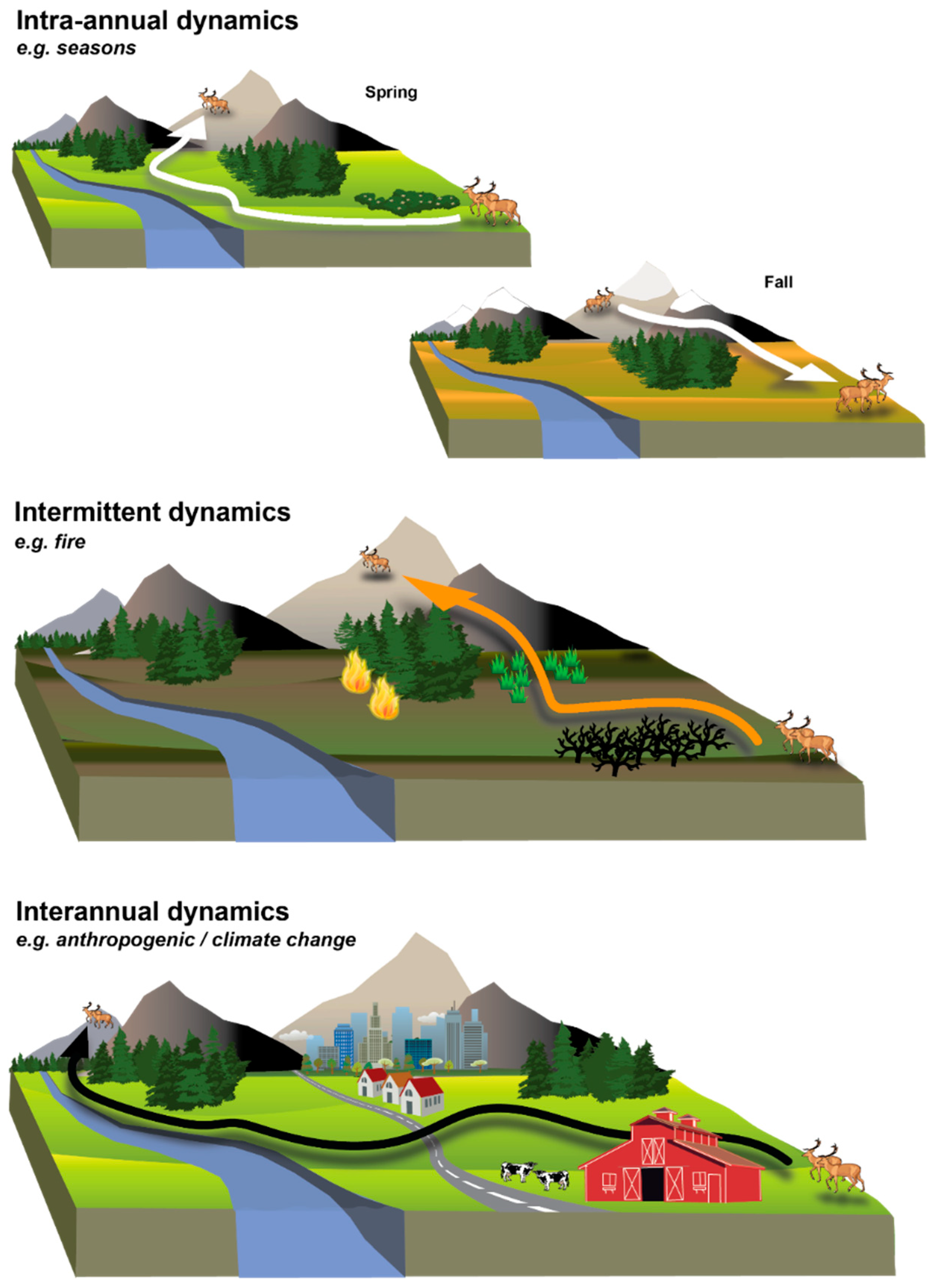
Figure 1.
Examples of dynamic landscape connectivity. Figure represents dynamic connectivity (lines with arrows) for a migratory ungulate. The area of land that supports connectivity changes depending on intra-annual dynamics such as seasons, intermittent dynamics such as disturbance, and interannual dynamics such as anthropogenic development and climate change. This figure is an illustrative example of only a few dynamics discussed in the paper. Please see text for additional information.

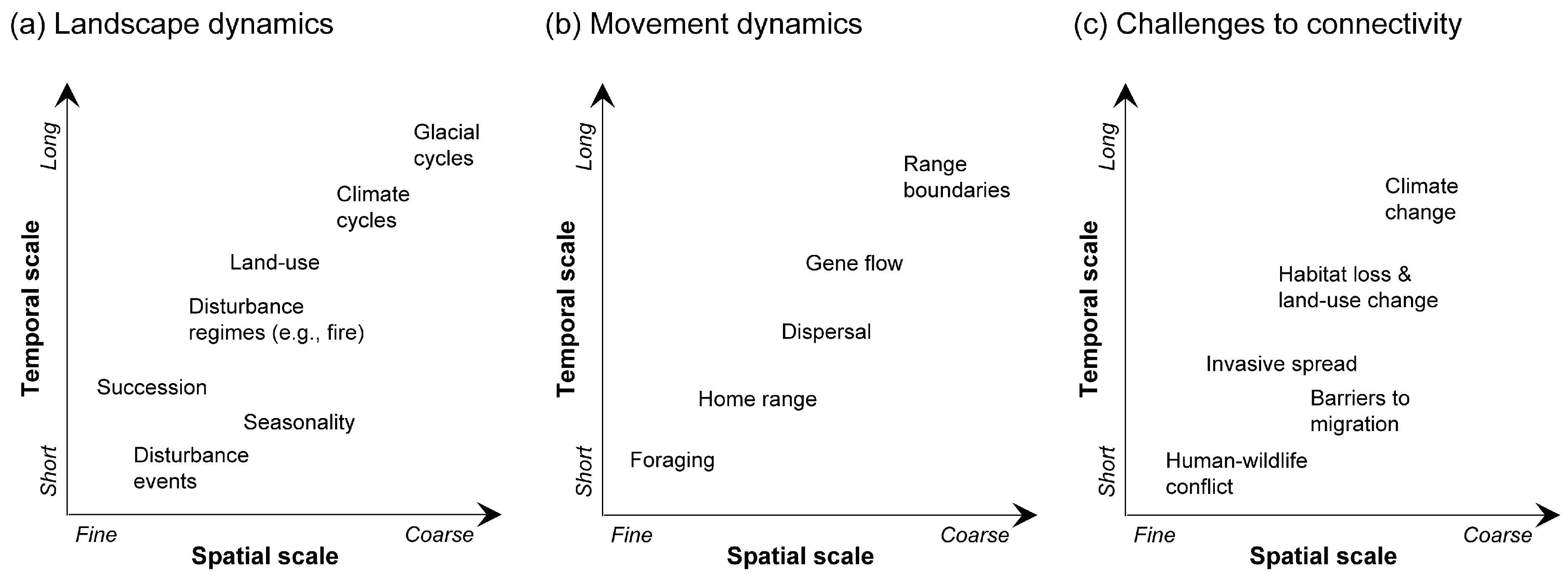
Figure 2.
Spatiotemporal scaling issues in dynamic landscape connectivity approaches. (a) Landscape dynamics, (b) movement dynamics, and (c) challenges to connectivity have processes at fine to coarse spatial scales over short to long temporal scales. The interplay of all three of these features drives dynamic landscape connectivity.

© 2020 by the authors. Licensee MDPI, Basel, Switzerland. This article is an open access article distributed under the terms and conditions of the Creative Commons Attribution (CC BY) license (http://creativecommons.org/licenses/by/4.0/).
Share and Cite
MDPI and ACS Style
Zeller, K.A.; Lewison, R.; Fletcher, R.J.; Tulbure, M.G.; Jennings, M.K. Understanding the Importance of Dynamic Landscape Connectivity. Land 2020, 9, 303. https://doi.org/10.3390/land9090303
AMA Style
Zeller KA, Lewison R, Fletcher RJ, Tulbure MG, Jennings MK. Understanding the Importance of Dynamic Landscape Connectivity. Land. 2020; 9(9):303. https://doi.org/10.3390/land9090303
Chicago/Turabian StyleZeller, Katherine A., Rebecca Lewison, Robert J. Fletcher, Mirela G. Tulbure, and Megan K. Jennings. 2020. "Understanding the Importance of Dynamic Landscape Connectivity" Land 9, no. 9: 303. https://doi.org/10.3390/land9090303
Note that from the first issue of 2016, this journal uses article numbers instead of page numbers. See further details here.