


Attribution and Causality Analyses of Regional Climate Variability

1
Max Planck Institute for Meteorology, 20146 Hamburg, Germany
2
Aerospace Information Research Institute, Chinese Academy of Sciences, Beijing 100101, China
3
Meteorologisches Institut, Universität Hamburg, 20146 Hamburg, Germany
4
Key Laboratory of Transportation Meteorology of China Meteorological Administration, Nanjing Joint Institute for Atmospheric Sciences, Nanjing 210041, China
*
Authors to whom correspondence should be addressed.
Land 2023, 12(4), 817; https://doi.org/10.3390/land12040817
Submission received: 30 December 2022
/
Revised: 4 February 2023
/
Accepted: 29 March 2023
/
Published: 3 April 2023
Abstract
:A two-step attribution and causality diagnostic is designed by employing singular spectrum analysis to unfold the attributed climate time series into a trajectory matrix and then subjected to an empirical orthogonal function analysis to identify the evolving driving forces, which can finally be related to major climate modes through their independent frequencies by wavelet analysis. Application results from the arid and drought-prone southern Intermountain region of North America are compared with the climate or larger scale forcing diagnosed from slow feature analysis using the sources of the water and energy flux balance. The following results are noted: (i) The changes between the subsequent four 20-year periods from 1930 to 2010 suggest predominantly climate-induced forcing by the Pacific Decadal Oscillation and the Atlantic Multidecadal Oscillation. (ii) Land cover influences on the changing land cover are of considerably smaller magnitude (in terms of area percentage cover) whose time evolution is well documented from forestation documents. (iii) The drivers of the climate-induced forcings within the last 20 years are identified as the quasi-biennial oscillation and the El Niño–Southern Oscillation by both the inter-annual two-step attribution and the causality diagnostics with monthly scale-based slow feature analysis.
1. Introduction
Climate variability is often analyzed and interpreted in terms of stationary processes related to constant forcing with constant means and higher moments. However, climate variability is also a result of changing forces leading to changes in the statistics of the climate’s dynamics. Exploration of the origin of these forces based on direct and on inverse methods is important as these forces underlie the observed changes in global or regional climate statistics. Direct methods utilize regional and global climate models that are being forced by increasing or decreasing greenhouse gas concentrations, volcanic activity, land use change, or solar radiation, which affect the response of the dynamics (see, for example, [1,2,3]). For regional climate analysis, say on a watershed scale, it is the large-scale global circulation (observed or simulated) that provides the climate-induced forcing of a nested smaller scale model (see, for example [4]).
Inverse methods explore the non-stationary forcing of climate variations, which are represented by a time series of an ecohydrological variable or by trajectories in a suitable state space. Physical or statistical models are introduced with the aim of assimilating the time changes or time-derivatives as they are responding to the underlying driving forces. Conventionally, such analyses determine the system’s sensitivity (in terms of metrics like elasticity, susceptibility, and resilience) or utilize (stationary) linear response theory (see, for example, [5], for a highly advanced review on ocean variability). Slow feature analyses cannot separate forcing into climate- and land cover-induced causes but can identify the processes responsible for the long-term rates of change (or time derivatives) by separating the slowly evolving driving forces from fast varying signals; this is a time series diagnostic of the climate-induced large scale attribution. First, analyses have been applied to single climate-related variables (see [6,7]); only Zhang et al. [7] focus on rainfall forcing as the water supply on a regional or watershed scale.
Here, we introduce a novel two-step attribution and causality analysis to determine the forces underlying the Earth’s varying ecohydrology on regional or watershed scales and to compare the results with using slow feature analyses. This is based on the surface water and energy balance, whose contributing fluxes constitute the rainfall–runoff chain, that are subjected to an attribution and causality analysis of the changes that have occurred. The attribution analysis, which separates the external or larger scale climate forcing from the land cover-induced driving, is based on a diagnostic climate forcing model ascribed to water and energy supply (precipitation and net radiation), while the partitioning of both evaporation-runoff and latent-sensible heat fluxes are affected by land cover forcing. Some first applications are noted: while Tomer and Schilling [8] have introduced this as an attribution approach of climate and land cover separation, variants of this have been applied to US-American and European watersheds by Renner et al. [9], watersheds of the Tibetan Plateau, South America, and a China–US-America comparison [10,11,12]. Following the attribution diagnostics, singular spectrum analysis and empirical orthogonal function analysis of inter-annual climate forcing identify the major climate modes through similar independent frequencies.
The aim of this paper is to interpret regional environmental change by attribution and causality analyses and to employ these to the water and energy fluxes governing the rainfall–runoff chain. The first step is the attribution analysis (employing a quasi-stationary diagnostic model to obtain suitable ecohydrological variables and their change in time) to separate external climate from internal land cover forcing (Section 2.1, see [11,12] as early applications of this scheme). Here, the time changes are quantified in terms of relative magnitudes comprising the total changes. However, this approach is not sufficient to fully explore the background of these changes. This requires a second step based on wavelet analysis, which has been shown to be able to extract various timescales underlying the forcings embedded in time variability [13,14]. Note that both attribution and its subsequent spectral causality analysis (empirical orthogonal function, EOF) are employed directly to (the time series of) ecohydrological state changes. This is in contrast (or in comparison) to a causality analysis based on slow feature analysis, which is employed directly to the time series of surface water and energy fluxes (and not their changes) which represent the sources of energy and the water cycle, that is, net radiation and precipitation. Here, a statistical forecast model needs to be constructed to provide the required time series of state changes, before it can be subjected to the spectral causality analysis (by wavelets, see [6], not unlike the final step following the attribution analysis.
The southern Intermountain region of North America (Arizona, Colorado, New Mexico, and Utah) is chosen to demonstrate the attribution and causality analysis of the observed regional environmental variability (Section 3). A summarizing discussion (Section 4) evaluates this framework for attribution and causality analysis of environmental change.
2. Methods: Attribution and Causality Analysis in Ecohydrological State Space
Atmosphere, biosphere, and pedosphere are linked by the rainfall–runoff chain, which is characterized by the land surface water and energy balances on a watershed. The external climate forces are precipitation and net-radiation P and N which, in equilibrium, are balanced by a partitioning of the remaining surface fluxes and coupled by an equation of state. The area-averaged long-term means of water and energy fluxes satisfy the respective balance equations and equation of state (all given in m/yr−1 as water equivalents of energy units). Note that the water equivalent in energy units is the amount of energy that is available to evaporate a certain amount of water. The conversion constant is the latent heat of water L = 2.5 × 10⁶ J kg−1.
P = Ro + E, N = H + E
The water and energy sources are precipitation P and net radiation N (left hand side), representing water supply and demand. The balancing fluxes (right hand side) partition runoff Ro and evapotranspiration E, or sensible heat H and evapotranspiration E, and are affected by internal or land cover-induced processes. Finally, an equation of state,
Ro = P exp(−N/P)
characterizes ideal land surface climate regimes which, like the ideal gas law, has been discovered empirically [15], interpreted by [16] and later theoretically derived [17]. Within the general Budyko framework, similar other relations are also suitable (see [18]).
Climate indices (flux ratios): The surface fluxes can be combined to non-dimensional flux ratio pairs to reduce the dimensions of the system to 2-dimensional spaces, where climate mean and their trajectories of change from watersheds could be embedded.
(i) Dryness: The dryness ratio or aridity index [19], D = N/P, relates water demand (energy supply) to water supply and characterizes the following biomes: tundra and forests, with D < 1/3 and 1/3 < D < 1, are energy-limited, while steppe and savanna, 1 < D < 2, semi-desert 2 < D < 3, and desert D > 3, are water-limited. This parameter lies in the center of our analysis which, from a climate system analysis point of view, characterizes wetter and drier climates at equilibrium balance with specific vegetation regimes. In contrast, drought and wetness are dominated by fluctuations inherent in atmospheric, agricultural, and hydrological aspects.
(ii) Energy excess: The energy flux ratio, U = H/N = 1 − E/N, of heat loss to energy supply describes the fraction of energy unused. That is, the portion of energy supply not being used for evapotranspiration from surface and thus, is available for direct sensible heating of the atmosphere, and also for photosynthesis [20].
(iii) Water excess: The water flux ratio of runoff to rainfall, W = Ro/P = 1 − E/P, connects blue water loss to total water supply, represents the fraction of water unused by an ecosystem [20] and is used to measure the watersheds’ efficiency, which characterizes the portion of water supply not being used by the ecosystem and, thus, is available for terrain formation.
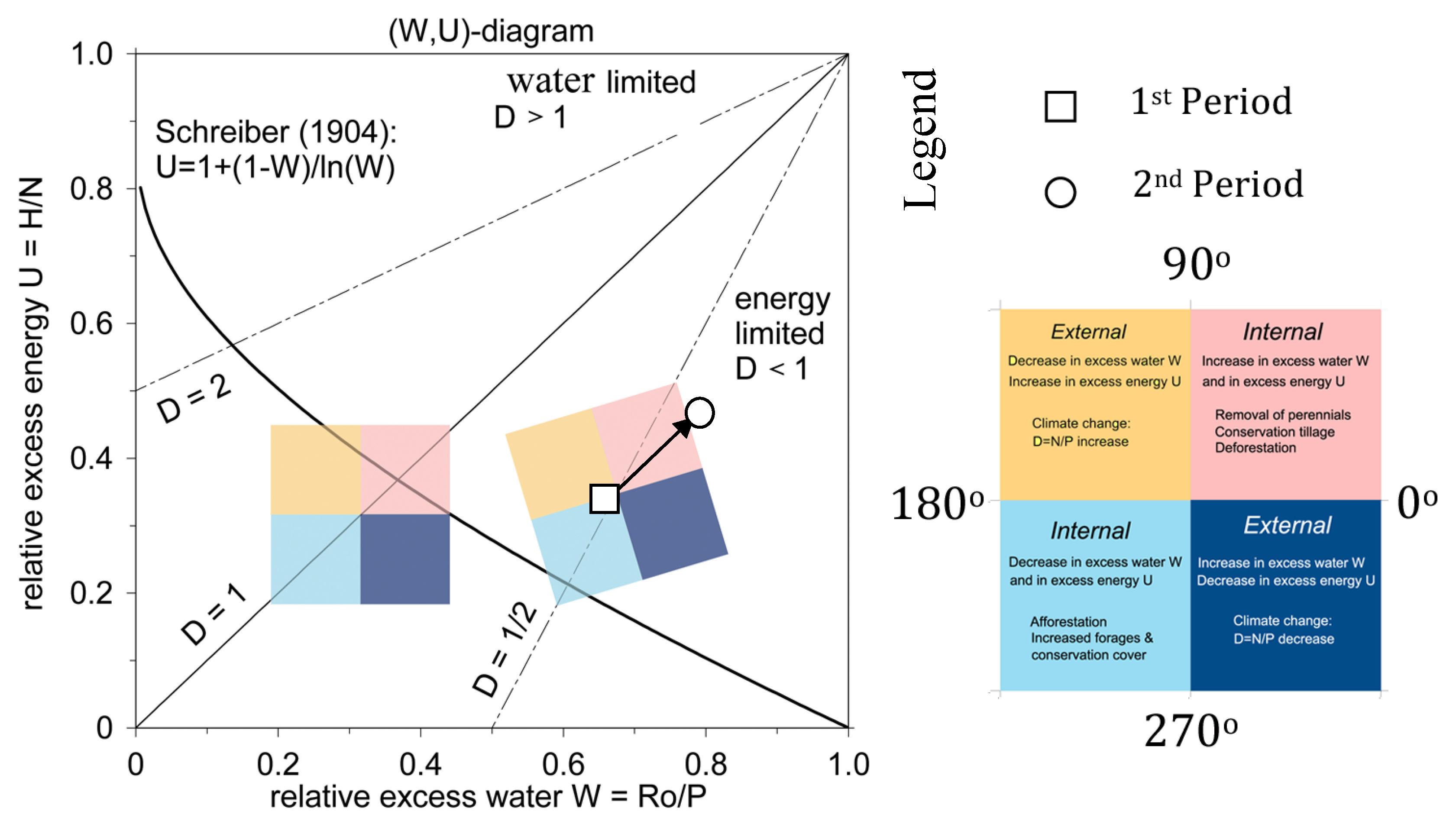
(iv) Both energy and water excess (or efficiency) describe proportions of available water and energy which, remaining unused, appear to be relevant for identifying the causes of climate and basin change. Note that U = H/N = 1 − E/N and W = Ro/P = 1 − E/P determine the dryness ratio, D = N/P = (1 − W)/(1 − U). Thus, the equation of state (2), W = Ro/P = exp(−N/P) or E/P = 1 – exp(−D) in the (E/P,D)-diagram, can be formulated as U = 1 + (1 − W) ln(W), which enters the ecohydrological state space or (U,W)-diagram (see [21]).
Fluxes and flux indices characterize the surface water and energy balance on a regional watershed scale as the key parameters, whose changes are subjected to attribution and causality analysis as described in the following section.
2.1. Attribution Analysis: Climate and Land Cover Forcing
In equilibrium, observed changes in water and energy storage are assumed to be zero in the long-term climatological mean. Changes from a first “equilibrium state” to another “equilibrium state” are applied to the attribution analysis as proposed by Tomer and Schilling [8]. Changes in the hydrological states must be caused either by a change in external climatic conditions, by changes in land cover conditions, or a combination of both. The conceptual model proposed by Tomer and Schilling [8] has great scientific appeal because of its potential to easily separate climatic from land cover effects on the water balance employing a diagnostic model (or scheme) to the trajectories in an ecohydrological state space (Figure 1, see also [8]) spanned by flux ratio (U,W)-coordinates. Here, the definition of climate changes only refers to climate changes if long-term annual average precipitation, P, or evaporative demand net radiation, N, were changing. All other potential impacts on evapotranspiration are referred to as internal land cover impact changes. For example, an increase in atmospheric CO2 concentrations, which supposedly affects evapotranspiration through the evaporative demand [22], cannot be attributed to a climate-induced change, but can be attributed to a land cover impact change.
Model construction: This technique separates external climate forcing from land cover-induced forcing. The latter changes the internal flux partitioning (between runoff, sensible, and latent heat fluxes), affected by land use and land cover modulation [11,12]. In this sense the Tomer–Schilling framework extends Budyko’s originally stationary state analysis to an attribution model of stepwise time changes (trends) between subsequent stationary states (Figure 1), which drive the climate and land cover changes. This concept provides a trajectory diagnostic [12] which, based on relative excess water and energy changes (dU = U2 − U1, dW = W2 − W1) separates water- and energy-related contributions into external and internal forcings measured in terms of direction and magnitude of the ecohydrological trajectories in the (U,W)-state space.
A gedanken experiment demonstrates how the ecohydrological attribution model provides the forces, which drive the observed changes of suitable ecohydrological indices, dU and dW, that is, pieces of their trajectory or, equivalently, their time derivative or change (Figure 1):
(i) Land cover-induced change (of land cover) is characterized by fixed climate forcing (P,N) = constant and greater than 0, which changes the excess energy U = (1 − E)/N and the water flux ratio W = (1 − E)/P, to dU = − dE/N and dW = − dE/P. That is, dE > 0 (< 0) gives (dU,dW) > 0 (< 0). That is, the change in (U,W)-diagram is directed to one of the two quadrants aligned along the main diagonal of internal partitioning: (dW,dU) > 0, or first quadrant (pink), and (dW,dU) < 0, or third quadrant (light blue).
(ii) Climate-induced changes fall into the off-diagonal quadrants. That is, the fourth quadrant (dW > 0, dU < 0, dark blue) and the second quadrant (dW < 0, dU > 0, yellow). Strictly, this attribution model holds for climate states along dU/dW~1 in the dryness range (0 < D < 2 to 3) characterized by tundra, forests, steppe and semi-deserts. That is, trajectories, for example along a Schreiber-type [18] curve describe climate forcing-induced change.
In general, in the Tomer–Schilling framework, land cover change (see also [23]) will affect the partitioning of latent and sensible heat fluxes and evapotranspiration and discharge, respectively, but not the climate-induced forcing by energy and water supply (net radiation or potential evapotranspiration and precipitation). Thus, land cover change will cause ecohydrological shifts in time toward an increasing or decreasing U and W, while changes in climate are related to increasing/decreasing dryness ratio D with an increasing W and a decreasing U, and vice versa.
An initial dryness ratio D1 (or origin) characterizing the ecohydrological climate state (D-slope in the (U,W)-diagram, Figure 1) which, associated with its subsequent state, provides a change of states (or trend, see [11]). All origins (U1,W1,D1) and their associated successive states define trajectory pieces, whose directions and magnitudes are measures of the attribution of change. Characterized by shift and rotation in the (U,W)-coordinate system, the attributions are classified stepwise (in terms of) in the rotating frame of reference (or quadrants) and their respective magnitudes can be quantified for each pixel i (or gridpoint) within the watershed or region:
dCi = dWi cos(θi − 90°) + dUi sin(θi − 90°)
dAi = −dWi sin(θi − 90°) + dUi cos(θi − 90°)
The angle θi = tan−1(1/Di) is given by the slope associated with the first period dryness, D1, in state space of pixel i: thus, external climate forcings (dCi) and internal or land cover forcings (dAi) are now traced in the related state space after subjecting (dUi,dWi) to the coordinate transformation given above [9,11,12]. That is, the attribution is now pixelwise quantified in terms of projected distances travelled by the trajectory of change along and across the dryness D1-line characterizing the pixel’s initial dryness ratio.
On climate time and regional watershed scale, which is assumed to change quasi-statically neglecting water and energy storage, we first employ the attribution analysis to all grid points (or pixel) individually, followed by watershed area averaging (<..>) to obtain representative (percent of area coverage) contributions of the components, dC = <dCi>, dA = <dAi>. These changes are measures of the attributed forcing (that is, time changes) describing the rainfall–runoff chain variability on a watershed scale.
2.2. Causality: Major Climate Modes
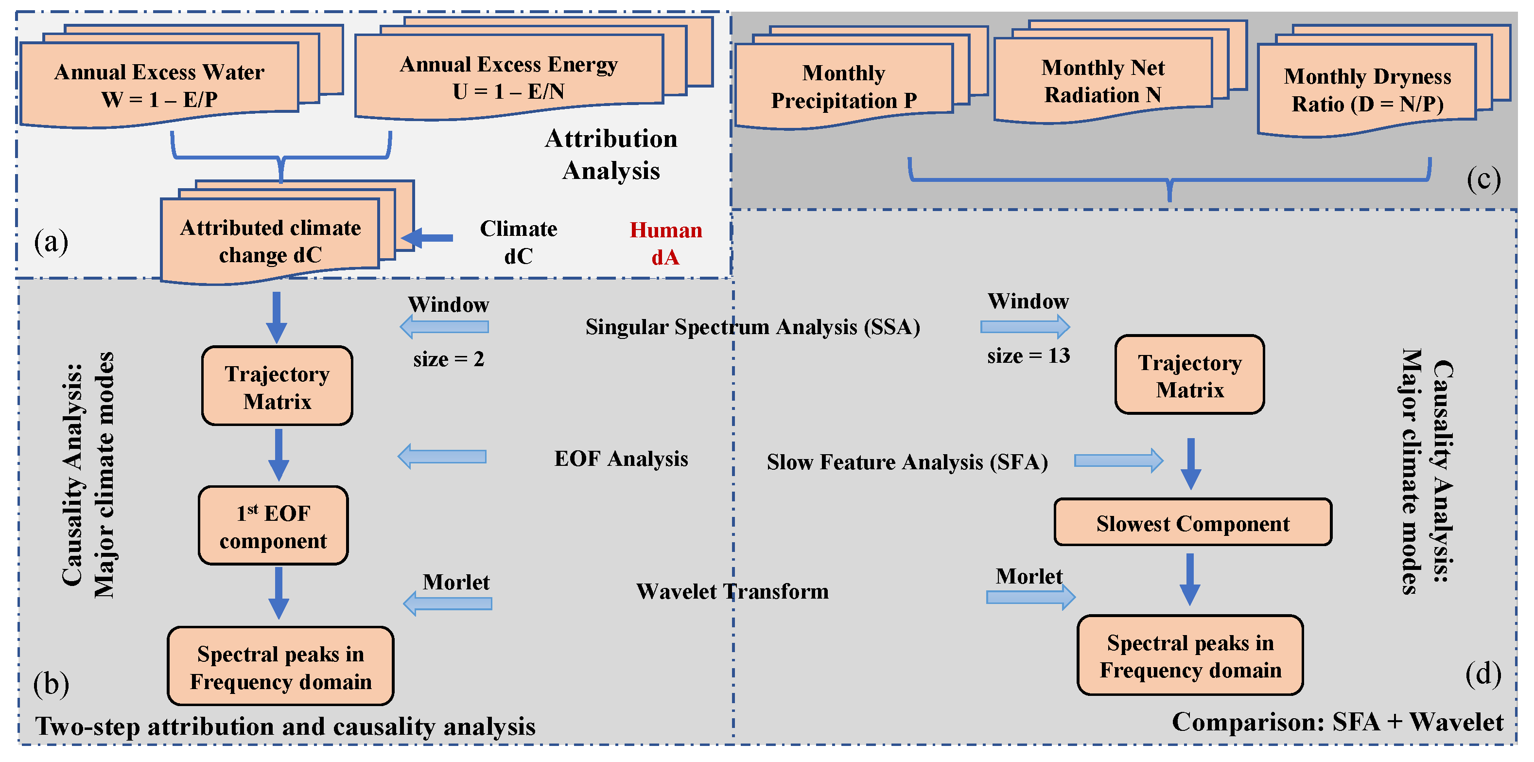
Besides long-term steady state changes being attributed to climate and land cover forcing, the inter-annual varying climate time series is subjected to a further causality analysis for diagnosing the driving forces of the larger scale climate modes (see flowchart, Figure 2). This inter-annual time series of the observed climate-attributed changes (or forcing) is subjected to singular spectrum analysis (SSA) to generate a trajectory matrix which, representing a causality pseudo state space, is subsequently interpreted after decomposition into empirical orthogonal functions (EOF).
For comparison, SSA and slow feature analysis (SFA, see [24]) serves as additional methods in which causality is applied to single variable time series of the source terms of the water and energy balance, namely precipitation, net radiation, and dryness ratio, to obtain a time series of the time changes of the single variable source term (or driving force). Thus, to obtain the forcing of the source terms the time series of their time changes need to be derived.
(i) A trajectory matrix (used as in singular spectrum analysis, SSA) is required for both the EOF decomposition and the SFA to describe the state evolution in terms of a window sliding over the time series. SSA is a non-parametric time series analysis method that unfolds an observed time series into a special structured matrix, called a trajectory matrix. The trajectory matrix has a Hankel structure whose off-diagonal elements are non-unique. Singular value decomposition is then applied to the trajectory matrix to extract time series structures, like EOF and SFA. The method can handle time series structures that include combinations of polynomials, sinusoids, and exponentials (see [25]).
(ii) The EOF decomposition requires a trajectory matrix of the attribution components (dC and dA), while the SFA requires a further model construction to obtain the time derivatives from a second-order polynomial (including fitting all linear and bi-linear interactions of both water and energy fluxes). Focusing on the climate or larger scale forcing beyond annual or seasonal cycles, window size m = 2 inter-annual attributed climate time series dC, and m = 13 months climate variable time series are used in EOF and SFA, respectively, for obtaining the SSA trajectory matrix and in order to be comparable.
(iii) The largest empirical orthogonal (or first EOF) of dC and the slowest SFA functions of climate variable are selected to obtain the required time series for a further time-frequency transform (wavelet analysis) to identify the major climate modes through similar frequencies. The sensitivity of the results could be tested by comparing them with previous research and an analysis of sliding and partly overlapping windows with window size m increasing.
SSA trajectory matrix and construction: For EOF-based causality, inter-annual climate-induced forcing dCi(t) from attribution analysis (Section 2.1) is selected to build the related SSA trajectory matrix, while for SFA-based causality, monthly variables of the ecohydrological source terms, P(t), N(t) or D(t) = N(t)/P(t) with t = t1, …, tn, are embedded in an N × m-dimensional state space spanned by m sliding window size (with t = t1, …, tN and N = n − m+1) to obtain a SSA trajectory matrix. Here, m represents the length of a window sliding across the time series, which corresponds to the time series of independent vector variables, X(t) = {x1(t), …, xm(t)} t = t1,...,tN. Now, an empirical model can be constructed to determine forcing or time change of the source terms.
For SFA-based causality, one more step of a K-dimensional function space is constructed to capture all possible linear and bi-linear interactions employing second-order polynomials (see [26,27]). H(t) = {h1(t), h2(t), …, hK(t)} t = t1,...,tN = {x1(t), …, xm(t), x21 (t), …, x1(t) xm(t), …, x2m−1(t), ..., x2m(t)} t = t1,...,tN, K = m + m(m+1)/2), which is 1-D of the following matrix eliminating null values:
Whitening or sphering, that is, normalization (to unit sphere with zero mean <h*j>, unit covariance <h*j h*jT> = 1, and division by standard deviation) replaces H(t) by H*(t) = {h*1(t), … h*K(t)}. A Python modular data processing toolkit (MDP) containing SFA can be found at: http://mdp-toolkit.sourceforge.net/ (last accessed on 15 March 2023).
Decomposition: For EOF-based causality, the SSA trajectory matrix X(t) is orthogonalized to provide the principal component-based reconstruction of the function space, which leads to climate or larger scale forcing, EOF1(t). As there are as many principal components as there are variables in the data, principal components are constructed in such a manner that the first principal component accounts for the largest possible variance in the data set. Then, all subsequent principal components are constructed with descending variance and being orthogonal to all preceding components, a conception that is well known in linear algebra as a multivariate eigenvalue problem [28,29,30].
For SFA-based causality, the normalized H*(t) is orthogonalized to Z(t) = {z1(t), …, zK(t)}, and then its time changes (or derivatives), Z’(t) are calculated to provide a K-dimensional non-stationary dynamical model of the time evolution of the time derivatives:
Z’(t) = {z’1(t), …, z’K(t)}.
Subjecting the time series of these time derivatives, Z’(t), to the Schmidt algorithm [31] occurs before calculating the time derivative KxK covariance matrix. The smallest eigenvalue and the corresponding eigenvector W1 provide the slow feature (large-scale) driving forces in terms of a projection of the previously orthogonalized time series Z(t). This serves as a natural low-frequency filter, and thus provides the slowest feature evolving as large-scale driving force.
y1(t) = W1·Z’(t).
It should be noted that further components, which capture forcings at other time scales, may also be included [32].
Generally, empirical orthogonal function analysis and slow feature analysis are unsupervised algorithms that learn linear and nonlinear functions to extract signals from input data. The basic idea is that its important characteristics remain predominantly unchanged in the actual time series, and the larger scale drivers can be identified by a statistical analysis to identify the frequencies of the driving forces from the observed non-stationary time series being linked to the dominating climate modes.
Time-frequency transform and harmonic analysis: Considering that the driving-force signal of a dynamic system often consists of different components with various timescales, time-frequency analysis of the first EOF component and of the SFA slowest feature exhibit the major modes of forcing by its independent frequencies. Wavelet variance of the scalar forcings (that is, the EOF principal component and the slowest component from SFA) provide a set of dominating modes of variability, from which those with independent frequencies define the underlying forcings to be interpreted by large-scale dynamics or drivers. Spectral peaks in frequency domain can be expressed as integral multiples of the same base periods. Here, Morlet wavelets, whose crucial parameter is the width of the Gaussian that tapers the sine wave, are used for time-frequency analysis of non-stationary time series data. A complex Morlet wavelet, w = exp(2iπ f t) exp(−½ t2 σ−2), can be defined as the product of a complex sine wave and a Gaussian window with the imaginary part i = √−1, frequency f in Hz, time t, and the width of the Gaussian, σ = ½ n / (π f).
3. Results: Application to the Southern Intermountain Dry Region of North America
Arizona, Colorado, New Mexico, and Utah comprise the southern Intermountain dry region of North America (except for Nevada and Wyoming, Figure 3). In terms of area cover, grassland is the dominant land-use class (57 percent), followed by forest land (21 percent) [33]. Reanalysis records of the southwestern United States from 1900 to 2010 are downloadable from the ERA-20CM dataset, which contains an ensemble of 10 atmospheric model integrations. The ensemble mean of the 10 ensemble members are finally employed to represent the ERA-20CM reanalysis with a horizontal resolution of 0.75° × 0.75°. The analysis involves using monthly, annual, and 20-year climatological means for all individual grid points, which are then spatially averaged over the four southern Intermountain states. When using the ERA-20CM dataset, it is important to take note of certain drawbacks in its precipitation data. Firstly, extreme precipitation events may be underestimated at the level of individual grid-points, but this does not affect area-averaged values. Secondly, Nogueira [34] has demonstrated that ERA-20CM tends to overestimate oceanwide climate mean precipitation when compared to satellite-based data like the GPCP. Thirdly, the German Weather Service has detected significant discrepancies in regions with high ground-based precipitation totals, such as rainforest areas.
3.1. Climatological Setting and Data
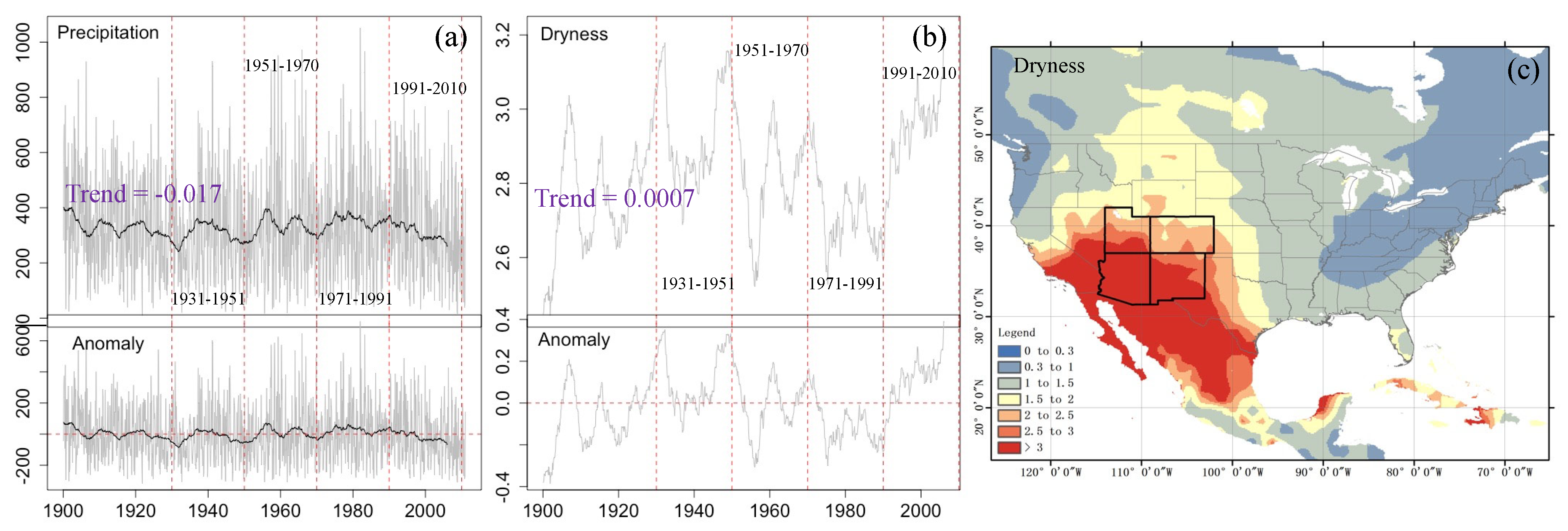
Over the southern Intermountain dry regions, ERA-20CM precipitation indicates a long-term linear regression trend of −0.017 mm/111year, while these non-cyclic trends in the dryness ratio are hardly to be noticed (0.00007 mm/111 year). The four Intermountain states are water-limited and characterized by dryness ratios exceeding D > 2, that is semi-desert and desert type climates according to the Budyko classification (Figure 3). Three temporal scales are used for attribution and causality analysis:
- (i)
- The decadal scale with non-overlapping 20 years’ state space of change (see Section 3.1) provides the basis for attribution and for causality analysis on very long time scales;
- (ii)
- the annual scale with overlapping m = 2 inter-annual attributed forcings; and
- (iii)
- the monthly scale with overlapping m = 13 months climate parameter time series (see Section 3.2) for causality analysis.
3.2. Attribution Analysis: Internal and External Forcings
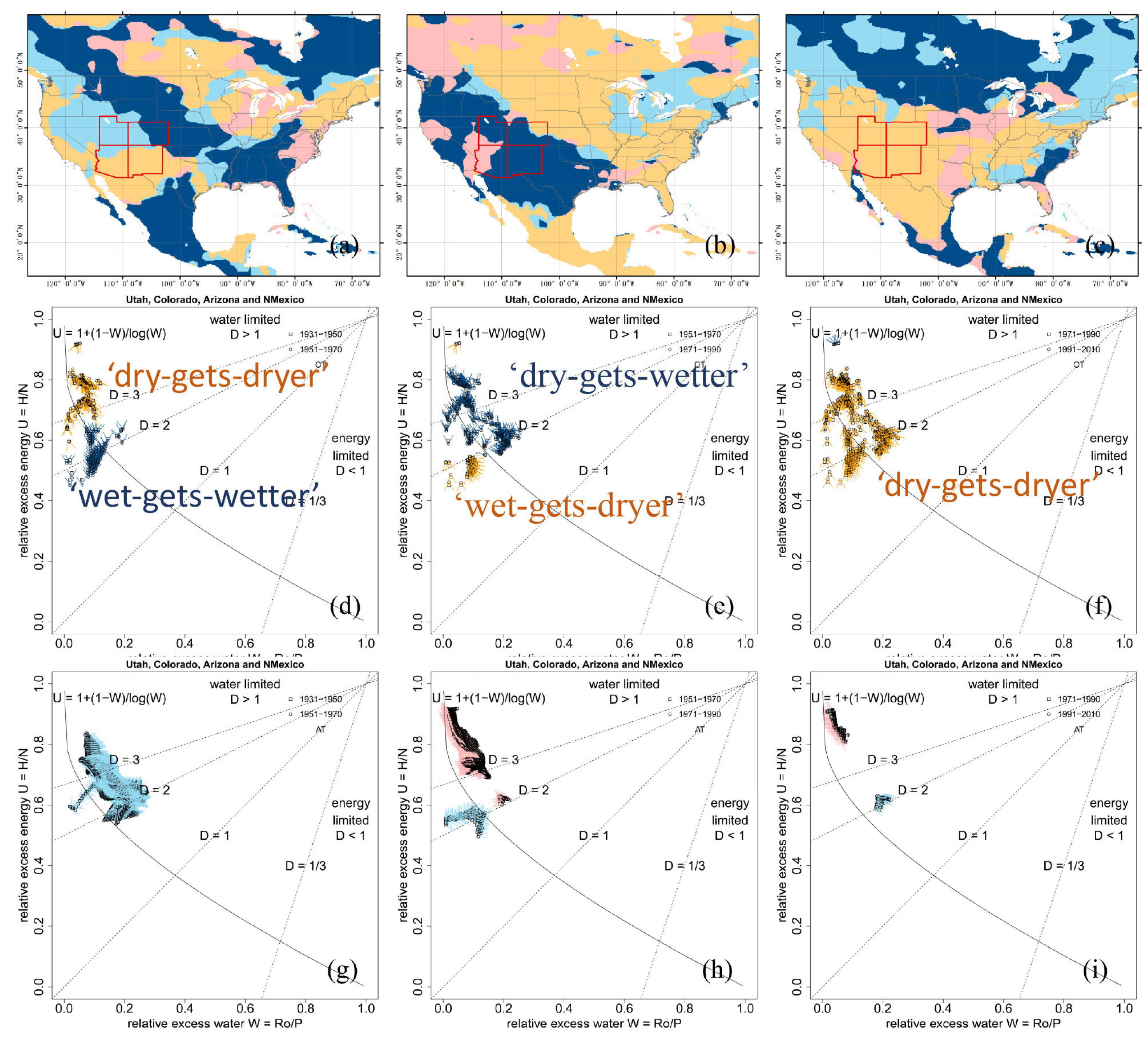
To analyze the observed quasi-stationary variability on a regional scale, four 20-year time intervals were examined to determine the conditions of change from drier to wetter (or vice versa) epochs. The analysis encompasses the entire North American continent as a geographical setting, with the southwestern states of Arizona, Colorado, New Mexico, and Utah being embedded within it (Figure 4a–c). However, all state space plots and statistics are calculated specifically for the southwestern states (Figure 4d–i). The following results are noted:
- (i)
- The area-averaged annual mean values of dryness (and precipitation) from the past 100 years reveal droughts before the 1910s, in the 1930s, from 1950 to 1970, and at the beginning of the twenty-first century (Figure 3a,b). Three changes between subsequent 20-year periods were observed: 1931–1950 and 1951–1970 (from wet to dry), 1951–1970 and 1971–1990 (from dry to wet), and 1971–1990 and 1991–2010 (from wet to dry).
- (ii)
- The external climate- and internal land cover-induced forcing of observed quasi-stationary changes on the regional scale were separated, as described in Section 2.1. Changes in the geographical and ecohydrological state space for all grid points are demonstrated in Figure 4 and summarized as southern Intermountain averages (see statistics in Figure 4).
Both climate- and land cover-induced forces govern all three periods of change, but there are notable differences (Figure 4), which are also quantified in the statistics presented in Figure 4:
From 1931–1950 to 1951–1970: About 60% (40%) of change is attributable to climate (land cover) forcing. The climate factor follows the regime of change “dry-gets-drier” (for deserts D > 3) and “wet-gets-wetter” (for steppe 2 < D < 3) separated at the (D = 3)-threshold between desert and semi-desert. The land cover-induced change occurs in both desert and semi-desert climates and is attributed to processes like afforestation and conversion on federal lands; that is, when the US’ forested areas have increased in the second period (beginning of the 50ies to the 60ies) reaching a peak of 3.02 million square kilometers (see [33]).
From 1951–1970 to 1971–1990: About 80% (20%) of change is attributable to climate (land cover)-induced forcing. Here the climate factor follows the dominating (>75%) regime change “dry-gets-wetter” (for D > 2) and only a small portion follows “wet-gets-drier” (D < 2). The land cover-induced change can be almost solely associated with deforestation-like affects, which is in agreement with forest area declining to 2.98 million square kilometers by the beginning of the 1990s [33].
From 1971–1990 to 1991–2010: About 100% of change is attributable to the climate-induced forcing following the “dry-gets-drier” regime extending throughout the water-limited regime (D > 1, Figure 4c). The negligible contribution by land cover-induced forcing of change shows in the history record in the way that the US’ forested area increased during the 1990s. Near the end of the 1990s, the area had decreased by 1% from the beginning of the 1950s, and 2% less since the end of the 1930s.
In general, the climate change trajectories (dark blue and yellow arrows), like “dry-gets-drier” and “wet-gets-wetter” dipole, are displayed in (U,W) state space and understandable through associating it with dryness changes (see Figure 4). This dipole has also been indicated in previous papers and has been used as a way to understand the opposed changes between the subperiods. For example, a pronounced “dry-gets-drier” and “wet-gets-wetter” dipole characterizes the significant changes in the Amazon region that covers large parts of the South American continent (1982 to 2006, see [11]). This is associated with a pronounced atmospheric circulation mode which, characterized by a water-column dipole, reveals a “dry-gets-drier” and “wet-gets wetter” climate change pattern (see [35]). Xiong et al. [36] indicate that 27.1% of global land confirms the “dry-gets-drier” and “wet-gets-wetter” dipole from 1985 to 2014, which is associated with water storage changes. Chen et al. [37] interpret the dipole in terms of the difference between precipitation and evaporation P−E, which represents the increase in atmospheric water vapor in humid regions under a warming climate and vice versa.
The attribution statistics (Table 1) reveal that the area-averaged climate changes (yellow = dryness increases, dark blue = wetness increases) suggest a 20 to 30 years’ periodicity as indicated by the dry-wet-drier and vice versa changes as described above. The related climate-induced processes affecting this region are the Pacific Decadal Oscillation (PDO), with warm or cold phases persisting for about 20–30 years, and the Atlantic Multidecadal Oscillation (AMO), with a characteristic period of 50–70 years [38,39,40]. Other climate or larger scale forcing within the 20-year interval length requires further causality analysis (following section). Note that the attribution analysis cannot quantify the contributions of PDO and AMO, since we only see a superposition of these two oscillations. It is beyond the scope of this study.
In summarizing: (i) the attribution analysis based on the Budyko framework separates climate processes from land cover forcing following the Tomer–Schilling [8] approach, quantifying the relative area cover affected by the intensity of the different causes of ecohydrological change and, thus, provides a proper metric characterizing a region or watershed. The attribution analysis reveals either climate- or land cover-induced forcing as a dominating contribution, and the latter can be confirmed using administrative documents. In the Intermountain regions, the relative area cover affected by the intensity of land cover activities decreased during the first period of change, 1931–1950 to 1951–1970, which coincides with local observations of area changes in land uses. Land used for recreation and wildlife areas (industrial and miscellaneous farmland use) expanded (declined) from 1945 to 1997 with an increase (decrease) of 73 (10.1 and 8) million acres, primarily in Arizona and Nevada. The increase is related to land-use conversions on federal lands, which had previously been forest as well as grassland pasture and range uses [41].
(ii) The results of the one-step quasi-stationary attribution analysis have also shown that the climate-related variability may be related to multi-decadal fluctuations with periods of about 20 to 30 years and 50 to 70 years, which may be related to the Pacific Decadal Oscillation, PDO) and the Atlantic Multidecadal Oscillation (AMO), respectively [38,39,40]. Climate-induced changes of the rainfall–runoff chain lasting from the 1950s to the 1970s are mainly related to the ecohydrological regime changes “dry-gets-wetter” (for D > 2) and only a small portion follows the “wet-gets-drier” regime shift (D < 2).
3.3. Causality and Climate Modes
EOF and SFA are applied for further extraction of the climate driving forces (see Section 2.2) with the time series characterizing ecohydrological state changes measured by the surface water demand, supply and the related fluxes, which represent the sources of the water and energy cycle, respectively. Then, the extracted climate driving forces are subjected to wavelet analysis for revealing possible strong and significant peaks, and for characterizing the time-scale structure in period (or frequency) and amplitude. Note that, in the EOF analysis, annual and seasonal cycles are removed by singular spectrum analysis unfolding the inter-annual attributed climate change time series into a trajectory matrix with the window size of m = 2 that overlaps years [42]. Furthermore, by definition, long-term trends do not play a role in determining driving forces. SFA analysis directly extracts the slowly varying features from a fast-varying input signal [30].
The EOF-based causality analysis (Figure 5a, based on the bi-annual embedding dimension, Figure 5) leads to the following results:
(i) Based on the bi-annual (m = 2) window sliding across the climate attributed time series, three significant dominant spectral peaks of variability are diagnosed as 3.47 years (2.07 to 4.13), 5.84 years (4.91 to 6.95), and 8.26 years.
(ii) The wavelet variance depending on timescale [6], see also (Wang et al. 2016) and (Jiang et al. 1997) reveals dominating or basic modes less than 3, which are related to the cycle of the biennial annular mode oscillation (BAMO, see [43]) and the quasi-biennial oscillation (QBO, around 28 months, see [44]). The modes 3.47 years and 5.84 years coincide with the intrinsic inter-annual variability of ENSO activities of every 2–7 years.
(iii) The spectral peak sensitivity is tested by increasing m, the window sliding size across the time series, which indicates that the larger m, the stronger the high frequency peaks are approaching a single one that represents BAMO and QBO (i.e., m = 6, peak = 2.16 yrs; m = 10, peak = 2.25 yrs; m = 15, peak = 2.37 yrs). This is the dominant pattern of variability in the tropical stratosphere and displays alternating downward-propagating easterly and westerly wind regimes. Still, the m value equal to 2 brings us closest to SFA results (see the following).
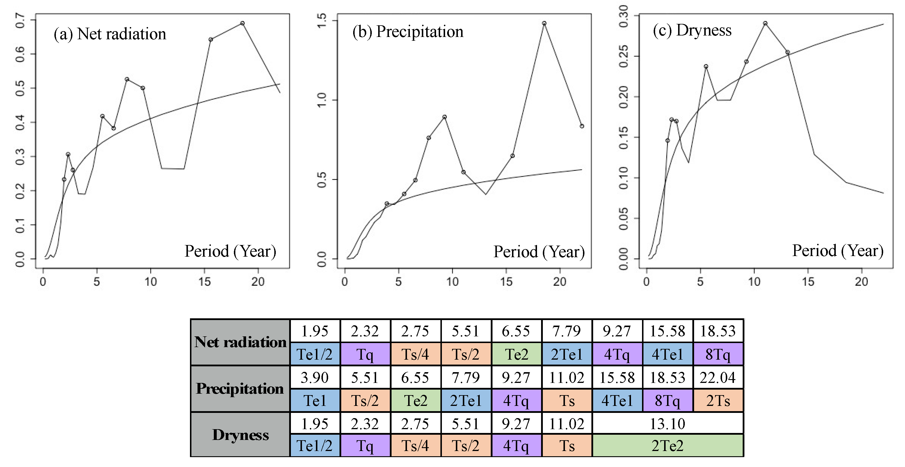
Zhang et al. [6] analyzes the precipitation records of the same four states as provided by the National Oceanic and Atmospheric Administration (NOAA)/National Climatic Data Center (consisting of 1440 months covering the period from January 1895–December 2015) and reveal similar dominating large scale climate forcing. Pan et al. [45] apply slow feature analysis (SFA) and wavelet transform directly to monthly mean indices (the El Niño–Southern Oscillation (ENSO), the Pacific Decadal Oscillation (PDO), the North Atlantic Oscillation (NAO), and the Atlantic Multidecadal Oscillation (AMO), etc.) developed and provided by the NOAA, which could represent independent variables related to regional climate variability. Their results suggest that the base periods and their harmonic oscillations are related to QBO, ENSO, and solar activity, and act as key connections among the climatic modes with synchronous behavior, highlighting the important roles of these three oscillations in the variability of the Earth’s climate. The SFA-based causality analysis in this study (embedding dimension of about 1 year with m = 13 months, Figure 6 and Figure 7) leads to the following results. For the sake of convenience, the base peak periods and their corresponding harmonic periods are denoted by integral multiples of Tq (purple), Te1 (blue), Te2 (green), and Ts (orange), respectively, according to [45].
(i) The SFA analysis of the dryness ratio D (P and N) reveals three (four and two) significant dominant spectral peaks of variability. Spectral peaks of the SFA-derived signals from the regional water supply can be expressed as integral multiples of the same base periods.
(ii) The wavelet variance depending on timescale ([6], see also [26] and [42]) reveals four dominating or basic modes (i.e., 2.32, 3.90, 6.55, and 11.02 years), which are related to the variations in oceanic and atmospheric modes (see [45]).
(iii) These dominating or basic modes, except for 11.02 years, also suggest the biennial annular mode oscillation (BAMO), the quasi-biennial oscillation (QBO), and ENSO activities as the singular spectrum-based causality analysis suggests.
(iv) Although larger scale oceanic and atmospheric modes are suggested by the precipitation records of the southwestern United States provided by the National Oceanic and Atmospheric Administration (see [6], the independency test excludes those larger scale oceanic and atmospheric modes (see Table 1 in [45]).
In summarizing, the results of the one-step attribution analysis have shown that the climate-driven variability may be related to PDO period of about 20 to 30 years and the Atlantic Multidecadal Oscillation (AMO) with a characteristic period of 50 to 70 years. The results of the two-step causality analysis show that the basic periods of the climate-driven variability are due to independent periods associated with the BAMO, QBO and ENSO (see also [43]). A hypothetical mechanism is described, whereby the QBO of zonal winds in the lower tropical stratosphere alters the distribution of intense deep convection activity throughout the western tropical Pacific. Coupled with the annual cycle and heat accumulation in the warm western Pacific basin, these QBO-induced fluctuations in deep convection cause fluctuations in the Central Pacific trade winds and the Walker circulation, which in turn determine the occurrence of ENSO events in the tropical Pacific. The precipitation in the southwest of the US is in a subsequent causality connected with ENSO events. ENSO as one drivers of precipitation variability over the southwest of the US acts via zonal shifts in tropical Pacific deep convection that drive teleconnections through the response in the extratropical Rossby wave-trains, integrated vapor transport, and atmospheric rivers.
4. Discussion
Attributing land use and land cover environmental changes requires a convincing time-averaging interval to characterize the conditions of change from drier to wetter (or vice versa) climate conditions. Theoretically, this time scale can be estimated in terms of the mean value of a random walk length which, based on the mean of the expected maximum excursions of the random walk, provides a suitable climate-averaging time scale [46]. Based on eight 100-year time series of global annual mean quantities, average random walk lengths of 20 to 25 years for ocean and land are obtained characterizing the random variability of the climate on the scale of civilizations. Similarly, Sun and Wang [47] suggested 20-year time intervals to capture equilibrium state as well as the sensitivity of evapotranspiration to land surface changes and the sensitivity of external climate forcing to evapotranspiration changes. Thus, four 20-year time intervals were used to analyze the conditions of change from drier to wetter (or vice versa) of observed quasi-stationary variability on regional scale.
Different from logistic regression, GLM regression, or Granger causality analysis, the attribution and causality analysis introduced here requires the use of both climate forcing time series (independent variables) and climate component time series (dependent variables). The goal is to diagnose the background climate forcing behind local climate variability without prior knowledge. The variations in oceanic and atmospheric modes at different timescales significantly contribute to global and regional climate variability, resulting in trends, cycles, random walks, or combinations thereof in the dependent time series. Regressing non-stationary time series through logistic regression, GLM regression, or Granger causality analysis can lead to false results, so it is necessary to first transform the non-stationary time series into a stationary time series before applying the chosen regression (further information and causality analyses can be found in [48,49]).
The wavelet transform is utilized in this study to extract features from a time series, as it shows the variation (power) of a time series as a function of time and period. However, it may not be effective for feature extraction when there are strong annual or seasonal cycles in the time series. To resolve this issue, it is advisable to use a decomposition method, such as EOF or SFA analysis, prior to the wavelet transform to remove annual and seasonal cycles.
Therefore, a two-step attribution and causality analysis was introduced as an up-scaling approach to examine environmental changes. This method was applied to time series of land surface water and energy fluxes, which characterize the ecohydrology at a regional scale. The first step is an attribution model, which separates external climate influences from internal land cover causes of environmental changes related to land use and land cover. External climate processes indicate water supply and demand at a larger scale, while internal or land cover-induced forcing components describe the partitioning of evaporation and sensible heat or discharge fluxes at a regional scale, as well as smaller scales.
The subsequent causality analysis employs singular spectrum analysis to identify evolving driving forces and slow feature causality analysis (SFA) for non-linear analysis using area mean water supply/demand. The first EOF determines the inter-annual contribution of external climate processes, while the slowest forcing of SFA determines the time derivative.
5. Conclusions: Upscaling by Attribution and Subsequent Causality Analyses
The ecohydrological conditions on a watershed scale are defined by the rainfall–runoff chain that results from the interaction of surface energy and water fluxes. Changes in these conditions can be used to analyze:
- (i)
- The distinction between external climate changes caused by climate change (manifested by changes in precipitation and net radiation) and internal changes caused by human activities (which affect the partitioning of heat and water into latent and sensible heat fluxes and runoff); and
- (ii)
- The cause of external climate changes in the rainfall–runoff chain variables (changes in climate and water and energy sources) that are driven by larger scale climate shifts such as oceanic and atmospheric patterns or the solar cycle.
As an example, this two-step attribution and causality analysis and SFA diagnostic have been applied to the drought-prone regions of the arid water-limited southwestern US. The results indicate the quasi-biennial oscillation and the El Niño-Southern Oscillation as the drivers of the climate-induced forcings. However, without the first step of attribution (or SFA only), there is a missing 20 to 30 years’ periodicity as suggested by the dry-wet-dry, and vice versa, changes described above related to the Pacific Decadal Oscillation.
To summarize, the impact of large-scale climate modes on global and regional climate has been well-studied, but the challenge lies in understanding the key driving factors of these modes at a regional level. Simply establishing statistical relationships between climate indices is not enough to fully grasp the intricate physical interactions between the variables. The two-step attribution and causality analysis that focuses on fluxes and state changes provides a deeper understanding of the underlying physical processes and drives and can be useful in improving our knowledge of regional climate and adapting to it. This approach can be seen as a first step towards a more comprehensive data-driven attribution and causality analysis for environmental change, beyond the traditional hydrological techniques based on sensitivity and elasticity modules emerging from the Budyko framework. Further enhancement of the analysis, such as incorporating more dimensions like vegetation absorption, soil properties, and hydraulic conductivity, is desirable. While the link between specific spectral basic periods and phenomena like PDO and AMO seems logical, it needs to be verified in a subsequent study. The purpose of this study was to introduce a tool for evaluating the interactions of climate-related metrics across various timescales and to provide insights into the underlying circulation patterns. Further validation of the tool’s efficacy will require the use of other established statistical methods in a follow-up study.
Author Contributions
Conceptualization, D.C. and K.F.; data curation, D.C. and S.Z.; formal analysis, D.C. and F.S.; funding acquisition, D.C. and L.Y.; investigation, D.C., K.F. and F.S.; methodology, D.C. and K.F.; resources, D.C. and S.Z.; software, D.C.; validation, D.C., K.F. and F.S.; visualization, D.C.; writing—original draft, D.C. and K.F.; writing—review and editing, D.C., K.F., F.S. and L.Y. All authors have read and agreed to the published version of the manuscript.
Funding
This research was supported by the National Key Research and Development Project of China (Grant 2020YFC1521900), and by the Strategic Priority Research Program of Chinese Academy of Sciences, grant number XDA23100504.
Informed Consent Statement
Not applicable.
Data Availability Statement
Reanalysis records of the southwestern United States from 1900 to 2010 are downloadable from ERA-20CM dataset (https://apps.ecmwf.int/datasets/data/era20cm-edmo/levtype=sfc/, last accessed on 15 March 2023).
Acknowledgments
This research was supported by the National Key Research and Development Project of China (Grant 2020YFC1521901 and 2020YFC1521904 in 2020YFC1521900), and by the Strategic Priority Research Program of Chinese Academy of Sciences, grant number XDA23100504, and by the Max Planck Institute of Meteorology (D.C., K.F.), and the reviewers’ helpful suggestions are acknowledged.
Conflicts of Interest
The authors declare no conflict of interest.
References
- Bordi, I.; Fraedrich, K.; Sutera, A.; Zhu, X. Transient response to well-mixed greenhouse gas changes. Theor. Appl. Climatol. 2012, 109, 245–252. [Google Scholar] [CrossRef]
- Bordi, I.; Fraedrich, K.; Sutera, A.; Zhu, X. On the effect of decreasing CO2 concentration in the atmosphere. Clim. Dyn. 2013, 40, 651–662. [Google Scholar] [CrossRef]
- Zhu, X.; Bye, J.; Fraedrich, K.; Bordi, I. Statistical structure of intrinsic climate variability under global warming. J. Clim. 2016, 29, 5935–5947. [Google Scholar] [CrossRef] [Green Version]
- Zhu, S.; Remedio, A.R.C.; Sein, D.V.; Sielmann, F.; Ge, F.; Xu, J.; Peng, T.; Jacob, D.; Fraedrich, K.; Zhi, X. Added value of the regionally coupled model ROM in the East Asian summer monsoon modeling. Theor. Appl. Climatol. 2020, 140, 375–387. [Google Scholar] [CrossRef] [Green Version]
- Liu, Z. Dynamics of interdecadal climate variability: A historical perspective. J. Clim. 2012, 25, 1963–1995. [Google Scholar] [CrossRef]
- Zhang, F.; Lei, Y.; Yu, Q.-R.; Fraedrich, K.; Iwabuchi, H. Causality of the Drought in the Southwestern United States Based on Observations. J. Clim. 2017, 30, 4891–4896. [Google Scholar] [CrossRef]
- Zhang, F.; Yang, P.; Fraedrich, K.; Zhou, X.; Wang, G.; Li, J. Reconstruction of driving forces from nonstationary time series including stationary regions and application to climate change. Phys. A Stat. Mech. Its Appl. 2017, 473, 337–343. [Google Scholar] [CrossRef]
- Tomer, M.D.; Schilling, K.E. A simple approach to distinguish land-use and climate-change effects on watershed hydrology. J. Hydrol. 2009, 376, 24–33. [Google Scholar] [CrossRef]
- Renner, M.; Seppelt, R.; Bernhofer, C.; Schymanski, S. Evaluation of water-energy balance frameworks to predict the sensitivity of streamflow to climate change. Hydrol. Earth Syst. Sci. 2012, 16, 1419–1433. [Google Scholar] [CrossRef] [Green Version]
- Cai, D.; Fraedrich, K.; Guan, Y.; Guo, S.; Zhang, C.; Zhu, X. Urbanization and climate change: Insights from eco-hydrological diagnostics. Sci. Total Environ. 2019, 647, 29–36. [Google Scholar] [CrossRef]
- Cai, D.; Fraedrich, K.; Sielmann, F.; Guan, Y.; Guo, S. Land-cover characterization and aridity changes of South America (1982–2006): An attribution by ecohydrological diagnostics. J. Clim. 2016, 29, 8175–8189. [Google Scholar] [CrossRef]
- Cai, D.; Fraedrich, K.; Sielmann, F.; Zhang, L.; Zhu, X.; Guo, S.; Guan, Y. Vegetation dynamics on the Tibetan Plateau (1982 to 2006): An attribution by eco-hydrological diagnostics. J. Clim. 2015, 28, 4576–4584. [Google Scholar] [CrossRef]
- Maraun, D.; Kurths, J.; Holschneider, M. Nonstationary Gaussian processes in wavelet domain: Synthesis, estimation, and significance testing. Phys. Rev. E 2007, 75, 016707. [Google Scholar] [CrossRef] [Green Version]
- Schulte, J.A. Wavelet analysis for non-stationary, nonlinear time series. Nonlinear Process. Geophys. 2016, 23, 257–267. [Google Scholar] [CrossRef] [Green Version]
- Schreiber, P. Über die Beziehungen zwischen dem Niederschlag und der Wasserführung der Flüsse in Mitteleuropa. Meteorolog. Z. 1904, 21, 441–452. [Google Scholar]
- Ol’Dekop, E. On evaporation from the surface of river basins. Trans. Meteorol. Obs. 1911, 4, 200. [Google Scholar]
- Fraedrich, K. A parsimonious stochastic water reservoir: Schreiber’s 1904 equation. J. Hydrometeorol. 2010, 11, 575–578. [Google Scholar] [CrossRef]
- Andréassian, V.; Mander, Ü.; Pae, T. The Budyko hypothesis before Budyko: The hydrological legacy of Evald Oldekop. J. Hydrol. 2016, 535, 386–391. [Google Scholar] [CrossRef]
- Budyko, M. Climate and Life. Academic Press: Cambridge, MA, USA, 1974; Volume 18. [Google Scholar]
- Milne, B.T.; Gupta, V.K.; Restrepo, C. A scale invariant coupling of plants, water, energy, and terrain. Ecoscience 2002, 9, 191–199. [Google Scholar] [CrossRef]
- Fraedrich, K.; Sielmann, F.; Cai, D.; Zhu, X. Climate dynamics on watershed scale: Along the rainfall-runoff chain. In The Fluid Dynamics of Climate; Springer: Vienna, Austria, 2016; pp. 183–209. [Google Scholar]
- Gedney, N.; Cox, P.M.; Betts, R.A.; Boucher, O.; Huntingford, C.; Stott, P. Detection of a direct carbon dioxide effect in continental river runoff records. Nature 2006, 439, 835–838. [Google Scholar] [CrossRef]
- Peña-Arancibia, J.L.; van Dijk, A.I.; Guerschman, J.P.; Mulligan, M.; Bruijnzeel, L.A.S.; McVicar, T.R. Detecting changes in streamflow after partial woodland clearing in two large catchments in the seasonal tropics. J. Hydrol. 2012, 416, 60–71. [Google Scholar] [CrossRef]
- Wiskott, L. Slow Feature Analysis. In Encyclopedia of Computational Neuroscience; Jaeger, D., Jung, R., Eds.; Springer New York: New York, NY, USA, 2015; pp. 2715–2717. [Google Scholar]
- De Klerk, J. Adapting the singular spectrum analysis trajectory matrix technique to identify multiple additive time-series outliers. Stud. Econ. Econom. 2015, 39, 25–47. [Google Scholar] [CrossRef]
- Wang, G.; Yang, P.; Zhou, X. Extracting the driving force from ozone data using slow feature analysis. Theor. Appl. Climatol. 2016, 124, 985–989. [Google Scholar] [CrossRef]
- Yang, P.; Wang, G.; Zhang, F.; Zhou, X. Causality of global warming seen from observations: A scale analysis of driving force of the surface air temperature time series in the Northern Hemisphere. Clim. Dyn. 2016, 46, 3197–3204. [Google Scholar] [CrossRef]
- Fraedrich, K. Estimating the dimensions of weather and climate attractors. J. Atmos. Sci. 1986, 43, 419–432. [Google Scholar] [CrossRef]
- Fraedrich, K.; Wang, R. Estimating the correlation dimension of an attractor from noisy and small datasets based on re-embedding. Phys. D Nonlinear Phenom. 1993, 65, 373–398. [Google Scholar] [CrossRef]
- Vautard, R.; Yiou, P.; Ghil, M. Singular-spectrum analysis: A toolkit for short, noisy chaotic signals. Phys. D Nonlinear Phenom. 1992, 58, 95–126. [Google Scholar] [CrossRef]
- Pursell, L.; Trimble, S.Y. Gram-Schmidt Orthogonalization by Gauss Elimination. Am. Math. Mon. 1991, 98, 544–549. [Google Scholar] [CrossRef]
- Tsonis, A.A.; Pan, X.; Wang, G.; Nicolis, C. On the min–max estimation of mean daily temperatures. Clim. Dyn. 2019, 53, 1981–1989. [Google Scholar] [CrossRef]
- Alig, R.J. Land Use Changes Involving Forestry in the United States, 1952 to 1997, with Projections to 2050; U.S. Department of Agriculture, Forest Service, Pacific Northwest Research Station: Portland, OR, USA, 2003; Volume 587. [Google Scholar]
- Nogueira, M. Exploring the Links in Monthly to Decadal Variability of the Atmospheric Water Balance Over the Wettest Regions in ERA-20C. J. Geophys. Res. Atmos. 2017, 122, 10,560–510,577. [Google Scholar] [CrossRef]
- Bordi, I.; De Bonis, R.; Fraedrich, K.; Sutera, A. Interannual variability patterns of the world’s total column water content: Amazon River basin. Theor. Appl. Climatol. 2015, 122, 441–455. [Google Scholar] [CrossRef]
- Xiong, J.; Guo, S.; Chen, J.; Yin, J. A reexamination of the dry gets drier and wet gets wetter paradigm over global land: Insight from terrestrial water storage changes. Hydrol. Earth Syst. Sci. Discuss. 2022, 1–20. [Google Scholar]
- Chen, J.; Tapley, B.; Rodell, M.; Seo, K.W.; Wilson, C.; Scanlon, B.R.; Pokhrel, Y. Basin-scale river runoff estimation from GRACE gravity satellites, climate models, and in situ observations: A case study in the Amazon basin. Water Resour. Res. 2020, 56, e2020WR028032. [Google Scholar] [CrossRef]
- McCabe, G.J.; Palecki, M.A.; Betancourt, J.L. Pacific and Atlantic Ocean influences on multidecadal drought frequency in the United States. Proc. Natl. Acad. Sci. 2004, 101, 4136–4141. [Google Scholar] [CrossRef] [Green Version]
- Mo, K.C.; Schemm, J.-K.E.; Yoo, S.-H. Influence of ENSO and the Atlantic multidecadal oscillation on drought over the United States. J. Clim. 2009, 22, 5962–5982. [Google Scholar] [CrossRef] [Green Version]
- Zhu, K.; Guan, X.; Huang, J.; Wang, J.; Guo, S.; Cao, C. Precipitation over semi-arid regions of North Hemisphere affected by Atlantic Multidecadal Oscillation. Atmos. Res. 2021, 262, 105801. [Google Scholar] [CrossRef]
- Vesterby, M. Major uses of land in the United States, 1997; US Department of Agriculture, Economic Research Service: Washington, DC, USA, 2001. [Google Scholar]
- Jiang, J.; Zhang, D.e.; Fraedrich, K. Historic climate variability of wetness in east China (960–1992): A wavelet analysis. Int. J. Climatol. A J. R. Meteorol. Soc. 1997, 17, 969–981. [Google Scholar] [CrossRef]
- Johnstone, J.A. A quasi-biennial signal in western US hydroclimate and its global teleconnections. Clim. Dyn. 2011, 36, 663–680. [Google Scholar] [CrossRef] [Green Version]
- Baldwin, M.; Gray, L.; Dunkerton, T.; Hamilton, K.; Haynes, P.; Randel, W.; Holton, J.; Alexander, M.; Hirota, I.; Horinouchi, T. The quasi-biennial oscillation. Rev. Geophys. 2001, 39, 179–229. [Google Scholar] [CrossRef]
- Pan, X.; Wang, G.; Yang, P.; Wang, J.; Tsonis, A.A. On the interconnections among major climate modes and their common driving factors. Earth Syst. Dyn. 2020, 11, 525–535. [Google Scholar] [CrossRef]
- Bye, J.; Fraedrich, K.; Kirk, E.; Schubert, S.; Zhu, X. Random walk lengths of about 30 years in global climate. Geophys. Res. Lett. 2011, 38. [Google Scholar] [CrossRef] [Green Version]
- Sun, S.; Wang, G. Diagnosing the equilibrium state of a coupled global biosphere-atmosphere model. J. Geophys. Res. Atmos. 2011, 116. [Google Scholar] [CrossRef] [Green Version]
- Runge, J.; Bathiany, S.; Bollt, E.; Camps-Valls, G.; Coumou, D.; Deyle, E.; Glymour, C.; Kretschmer, M.; Mahecha, M.D.; Muñoz-Marí, J. Inferring causation from time series in Earth system sciences. Nat. Commun. 2019, 10, 2553. [Google Scholar] [CrossRef] [PubMed] [Green Version]
- Liang, X.S. Unraveling the cause-effect relation between time series. Phys. Rev. E 2014, 90, 052150. [Google Scholar] [CrossRef] [PubMed] [Green Version]
Figure 1.
Ecohydrological states in the (U,W)-diagram spanned by relative excess water W (runoff versus precipitation) and energy U (sensible heat flux versus net radiation), with lines of constant dryness D (net radiation versus precipitation). Ecohydrological states are denoted by squares and circles: the reference states (squares) represent the first period, which is followed by a subsequent shift to the second period (circles). Directions and lengths of arrows connecting first with the second period provide the attribution of change (see text): trajectories along (across) the main diagonal characterize a change of the internal (external) partitioning. The rainfall–runoff chain related to Budyko’s framework can also be included in the ecohydrological state space: U = 1 + (1 − W) ln(W).

Figure 2.
Flowchart of the two-step attribution and causality analysis on inter-annual scale (left, (a,b) versus slow feature analysis of causality on monthly scale (right, (c,d)). Input: ecohydrological indices and fluxes of water supply and demand (pink in (a,c)). Methods: attribution analysis (yellow in (a)) and causality analysis (blue in (b,d) with stepwise results (pink in (b,d)).

Figure 3.
Climatological setting of the southern Intermountain region (from ERA-20C): (a) area averaged monthly mean precipitation (in mm/year) time series (top) and anomalies with the seasonal cycle removed (bottom), both with 5–year moving averages (black line). (b) Area-averaged dryness ratio of net radiation over rainfall (D = N/P, 5–yr moving average), and (c) geographical distribution of dryness ratio. Note that linear regression trends are displayed in purple.

Figure 4.
Ecohydrological attribution analysis for the southwestern states of Arizona, Colorado, New Mexico, and Utah (step 1): geographical distributions of the four quadrants of attribution depending on the 20-year time changes from 1931–1950 to 1951–1970, 1951–1970 to 1971–1990, and 1971–1990 to 1991–2010 (1st row, (a–c)) as well as trajectories of changes in excess energy and water (U,W) for external climate forcing (2nd row, (d–f)) and for land cover-induced (internal) forcing (3rd row, (g–i)).

Figure 5.
The time−averaged power spectrum from Morlet wavelet transform of empirical orthogonal function (EOF, m = 2): (a) the EOF1 from the inter-annual climate component; (b) power spectrum of the wavelet transform coefficient for the reconstruction of the EOF1 (significant regions are surrounded by black isolines); and (c) time-averaged power spectrum. The periods (dots) which pass the significance test at the 0.05 significance level are listed and classified, including the biennial annular mode oscillation (BAMO), the quasi-biennial oscillation (QBO) and the El Niño–Southern Oscillation (ENSO).

Figure 6.
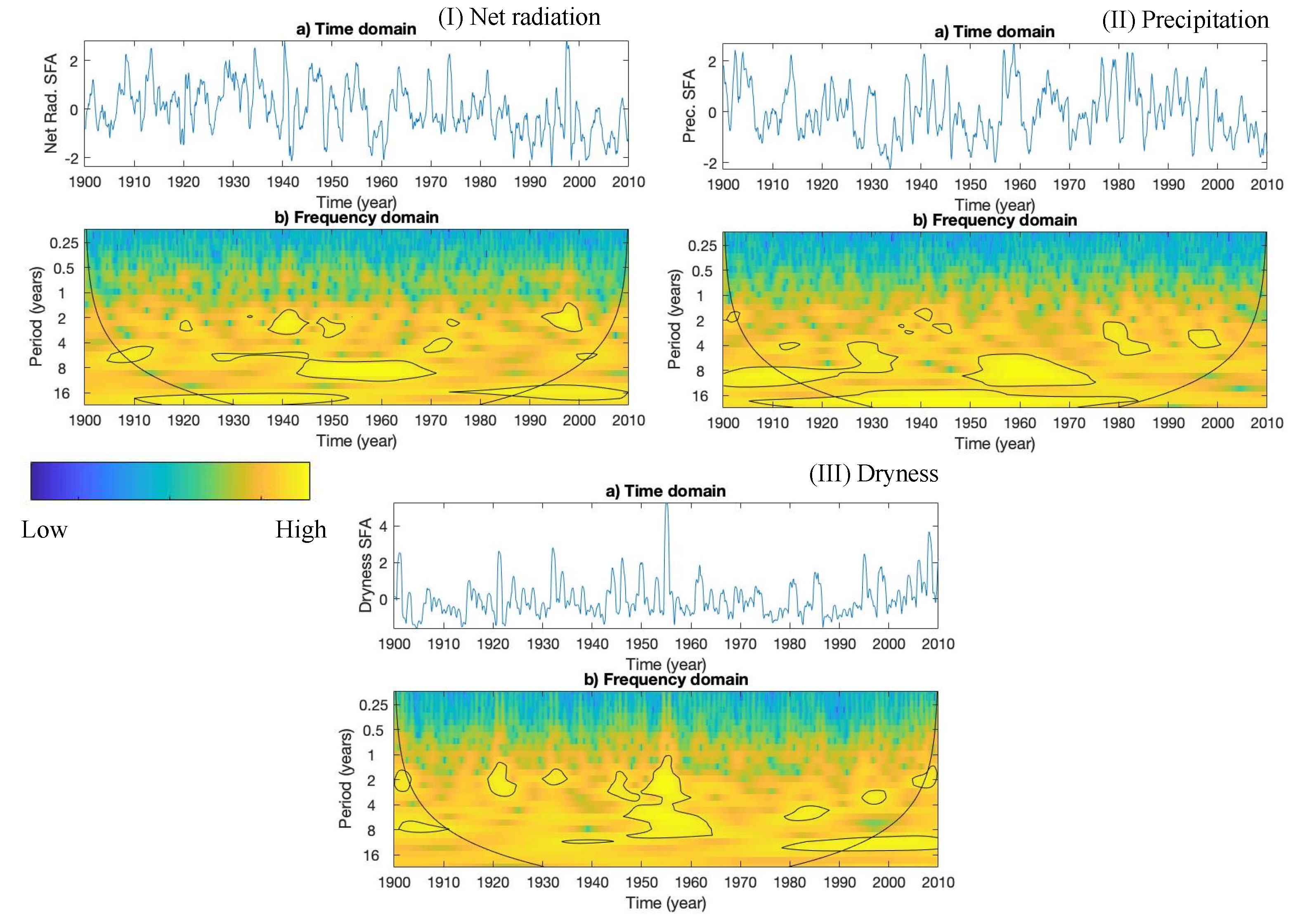
Time series of annual means of (a) the normalized driving force generated by slow feature signals when m = 13 and (b) the power spectrum of the wavelet transform coefficient for the reconstruction of the driving force for (I) net radiation, (II) precipitation, and (III) dryness ratio. Significant regions are surrounded by black isolines.
Figure 6.
Time series of annual means of (a) the normalized driving force generated by slow feature signals when m = 13 and (b) the power spectrum of the wavelet transform coefficient for the reconstruction of the driving force for (I) net radiation, (II) precipitation, and (III) dryness ratio. Significant regions are surrounded by black isolines.

Figure 7.
The time-averaged power spectrum from Morlet wavelet transform of SFA-extracted (m = 13) slow feature signals (jagged curves) for (a) net radiation, (b) precipitation, and (c) dryness. The significant points (dots) which pass the significance test at the 0.05 significance level (smooth line) are listed and classified, including the biennial annular mode oscillation (BAMO) and/or the quasi-biennial oscillation (QBO) in purple (Tq), the El Niño–Southern Oscillation (ENSO) in blue (Te1) and green (Te2), and sunspot cycle in orange (Ts).


Table 1.
This table quantifies the results presented in Figure 4 in terms of the respective areas (in percent) affected by the changing climate and land cover.
Table 1.
This table quantifies the results presented in Figure 4 in terms of the respective areas (in percent) affected by the changing climate and land cover.
| Attribution | 1931–1950 to 1951–1970 | 1951–1970 to 1971–1990 | 1971–1990 to 1991–2010 |
|---|---|---|---|
| dw > 0 & du > 0 | 0 | 16.07% | 1.49% |
| dw < 0 & du > 0 | 43.27% | 5.63% | 97.72% |
| dw < 0 & du < 0 | 41.71% | 1.37% | 0.37% |
| dw > 0 & du < 0 | 15.02% | 76.93% | 0.42% |
Disclaimer/Publisher’s Note: The statements, opinions and data contained in all publications are solely those of the individual author(s) and contributor(s) and not of MDPI and/or the editor(s). MDPI and/or the editor(s) disclaim responsibility for any injury to people or property resulting from any ideas, methods, instructions or products referred to in the content. |
© 2023 by the authors. Licensee MDPI, Basel, Switzerland. This article is an open access article distributed under the terms and conditions of the Creative Commons Attribution (CC BY) license (https://creativecommons.org/licenses/by/4.0/).
Share and Cite
MDPI and ACS Style
Cai, D.; Fraedrich, K.; Sielmann, F.; Zhu, S.; Yu, L. Attribution and Causality Analyses of Regional Climate Variability. Land 2023, 12, 817. https://doi.org/10.3390/land12040817
AMA Style
Cai D, Fraedrich K, Sielmann F, Zhu S, Yu L. Attribution and Causality Analyses of Regional Climate Variability. Land. 2023; 12(4):817. https://doi.org/10.3390/land12040817
Chicago/Turabian StyleCai, Danlu, Klaus Fraedrich, Frank Sielmann, Shoupeng Zhu, and Lijun Yu. 2023. "Attribution and Causality Analyses of Regional Climate Variability" Land 12, no. 4: 817. https://doi.org/10.3390/land12040817
Note that from the first issue of 2016, this journal uses article numbers instead of page numbers. See further details here.