
Effect of Barometric Pressure Fluctuations on Gas Transport over Soil Surfaces


School of Mathematics and Computer Science, Zhejiang A & F University, Hangzhou 311300, China
*
Author to whom correspondence should be addressed.
Land 2023, 12(1), 161; https://doi.org/10.3390/land12010161
Submission received: 6 November 2022
/
Revised: 28 December 2022
/
Accepted: 30 December 2022
/
Published: 3 January 2023
(This article belongs to the Section Land–Climate Interactions)
Abstract
:Molar diffusion mechanism is generally considered to be the main physical process of gas transport at the soil–atmosphere interface. However, the advection mechanism in porous medium can considerably affect soil gas transport. Barometric pressure fluctuations caused by pressure pumps is one of the main factors that affects the advection mechanism. Most of the existing studies are overly focused on the construction of complex mathematical models and cannot exclude other environmental factors from interfering. In the present study, a simple attenuation form of barometric fluctuations was explored as a “minimum unit” of pressure wave in laboratory. A pressure attenuation model (PAM) was developed to verify the relationship between pressure difference and gas emission from soil surface by measuring the change in pressure attenuation. The effect of pressure fluctuations on soil surface gas fluxes was then quantified based on the calculated fluxes. In addition, the relationship between the physical properties of the soil medium and the change in pressure was also analyzed. The results show that fluctuations in air pressure can cause a change in soil CO2 fluxes by an order of magnitude (change of 1 Pa can result in approximately 100% change in flux for sandy loam). The sensitivity of different soil medium to pressure differences was positively correlated with soil gas permeability, which is the main physical property of soil that influences the response of gas to pressure fluctuations. These results provide important prerequisites for quantifying more complex pressure fluctuations in a future study.
1. Introduction
Soil is one of the main sources of greenhouse gas (GHG) emission, which is a global climate issue. Accurate measurements of GHG fluxes (including, carbon dioxide, CO2; nitrous oxide, N2O; and methane, CH4) from the soil surface are important for assessing the global GHG budget and the effects of anthropogenic GHG emissions [1,2,3,4]. Furthermore, GHG fluxes also facilitate prediction of future trends of climate change at macro level.
When calculating gas fluxes in soil, two mechanisms that control gas transport—namely diffusion and convection—should be considered [5,6,7]. Diffusion is driven by gradient of gas concentration [4,7,8], whereas convection is the response of a gas to its density or pressure gradient [7,9,10]. During atmosphere-to-soil gas exchange, air temperature, wind, and air pressure can drive three different mechanisms of convective transport. These mechanisms include: (1) thermally-induced convection, a type of free convection that is triggered by an unsteady density gradient, which is caused by temperature differences within the atmospheric and soil envelope [11,12,13,14,15,16]; (2) wind-induced transport (WIT) is caused by surface winds in the boundary layer, which generate pressure differences or enhance the exchange between soil gases and the atmosphere due to the dispersion effect of the wind [7,17,18,19,20,21]; and (3) barometric induction is the movement of soil gases in the vertical direction due to changes in atmospheric pressure, which increases the rate of soil gas exchange. It is usually associated with barometric pressure changes of several hundred pascals over a few hours [22,23,24]. In addition to the above mechanisms, dispersion is also an important mechanism affecting soil gas transport, which is manifested as an enhancement of diffusion by shear forces. Depending on the flow rate of the gas in the soil, dispersion can be divided into two types [25]: (i) at low flow rates, where molecular diffusion makes the dominant contribution in mass transfer; and (ii) at high flow rates, where dispersion is more influenced by the tortuous paths in the soil. For the second type of dispersion, when the pressure gradient of the flow in the soil rotates with time, it is specifically referred to as “rotational dispersion” [26], a typical example is that the air turbulence passing through the soil, which causes increase or suppress to gas flux in soil surface. In the present study, we focused on the effects of changes in soil surface pressure (primarily, attenuation waves) on soil gas emissions as well as gas fluxes. The thermal convection was not considered when convection was equivalent to the advection term, which is used hereafter to describe convection. Meanwhile, the effect of air turbulence on the soil surface is not considered in this study, so the dispersion effect is ignored.
Several previous studies have reported that small changes in pressure can bring order of magnitude changes in soil gas fluxes [27,28,29,30]. Therefore, soil gas fluxes need to be calculated more accurately by investigating the relationship between soil gas transport and pressure in depth. Most studies on this topic are based on field and laboratory measurements, where field measurements are mainly used to analyze gas emissions by retrieving atmospheric and soil pressure fluctuations through a reference chamber, and the gas concentration distribution in the soil is calculated [31]. However, many uncontrollable environmental factors are present in field that can jointly affect the distribution of soil gas concentrations as well as gas emissions. Bain et al. [32] and Xu et al. [33] investigated the effect of wind-induced pressure differences on measured soil CO2 fluxes in the field based on closed chambers and found that a pressure difference of 1 Pa could result in a 100% increase or decrease in fluxes. Levintal et al. [7] collected soil to five vertical polyvinyl chloride (PVC) columns and explored the wind-induced pressure effect on CO2 flux in field, which shows an increase compared to diffusion flux from 25% to 500%. Poulsen et al. [30] analyzed an approximately 7 × 10 m site in Denmark, over a large area, in combination with measured data and concluded that a change in atmospheric pressure of 200 Pa could also cause an approximately 100% change in CO2 flux; by converting the site area to the size of the closed chamber area, it is consistent with the former results. Takle et al. [34] explored the effect of high-frequency pressure fluctuations on surface CO2 fluxes at farmland, and pressure pumps were found to cause 300–700% higher than pure diffusion flux. Kuang et al. [6] also reported that the radon gas flux at the surface is affected by pressure and varies from 10% to 200%. However, in practice, the field measurements of the above study cannot be absolutely and strictly controlled for variables, and factors, such as temperature and soil water content are temporally heterogeneous and spatially heterogeneous, which can cause bias in the estimation of flux effects. Hence, it is not easy to analyze the sole influence of pressure and give a relational model, leading to the inability to conduct studies in complex environments. Meanwhile, some scholars have studied the effect of pressure fluctuations on soil gas transport by a given barometric pressure change [35,36,37,38]. However, their studies are difficult to compare with field observations. First, some of the experiments used soil matrices with much higher porosity than natural soils—they used coarse sand and glass beads of a few millimeters in diameter. Moreover, the pressure variations that have been previously studied were in the form of sinusoidal waves, and only a few models have been given by Forde, Cahill, Beckie and Mayer [1], Laemmel, Mohr, Schack-Kirchner, Schindler and Maier [35], Scotter and Raats [38] to specifically describe the effects of pressure variations on gas emissions.
The present study used three common soil medium under laboratory controlled variables to: (1) construct a model of the relationship between pressure changes and gas emissions (PAM); (2) measure the enhancement or inhibition of CO2 fluxes in response to pressure changes; (3) compare the constructed model with other flux calculation methods, such as closed chamber method; and (4) analyze the relationship between soil physical properties and pressure changes.
2. Materials and Methods
2.1. Gas Transport Equation
In porous medium, such as soil, the response of gas to diffusion and advection can be described using the advection-diffusion equation (ADE) [23]. By neglecting the role of biological or chemical sources or sinks, the ADE in one-dimensional form can be formulated as:
where is the aerated porosity of soil (m3·m−3), is the effective diffusion coefficient of gas in soil (m2·s−1), is the gas flow rate in the medium (m·s−1), is the gas concentration (μ mol·m−3), is the time (s), and is the vertical distance of a point in the soil layer in the medium from the soil surface (m). Term I in Equation (1) is known as the transient term or storage term, which means that the concentration varies with time. Term II to the right of Equation (1) is expressed as the contribution of only molecular diffusion (i.e., diffusion term), as the disperation effect is ignored in this study, whereas term III is expressed as the contribution of advection (i.e., advection term).
2.2. Flux Calculation
2.2.1. Diffusion Flux
When molecular diffusion dominates the transport of gases in the soil and the gas concentration in the soil profile is in steady-state equilibrium, the diffusion flux of gases on the soil surface can be calculated from the soil gas concentration gradient using Equation (2) (Fick’s first law):
where is the diffusion flux (μ·mol·m−2·s−1), is the profile concentration gradient (μ·mol·m−4), and the negative sign indicates the diffusion of gas from high to low concentrations.
The effective diffusion coefficient of gases in soil can be estimated by combining molecular diffusion coefficients of atmospheric gases (m2·s−1) with the physical properties of soil. The physical properties of the soil are calculated using the Millington and Quirk model [39]:
where is the total porosity of the soil (m3·m−3) and for completely dry soil.
2.2.2. Advection Flux
If the ambient air pressure at the soil surface changes and creates a pressure difference between the surface and interior of the soil, advection will occur during the transport of gas in soil. This would affect the transport state of the gas and change the gas transport volume. According to Equation (1), the magnitude of advection flow (μ·mol·m−2·s−1) at the soil surface can be determined by multiplying the gas flow rate at the soil surface and the gas concentration at the surface:
As soil is a porous medium, gas flow in soil generally follows Darcy’s law. The gas flow velocity resulting from the pressure difference can be calculated using Equation (5):
where is the soil gas permeability (m2), is the aerodynamic viscosity coefficient (Pa·s), is the air pressure (Pa), and is the pressure gradient (Pa·m−1).
2.2.3. Total Flux
Considering the advection and diffusion contributions that were calculated using Equation (1), the total theoretical gas flux (μ·mol·m−2·s−1) emitted from the soil surface can be obtained as follows [40]:
In this study, we used Equation (6) to calculate the gas fluxes through the soil surface. It is worth noting that from Equation (1), the diffusion and advection flux in Equation (6) were multiplied with the aerated porosity, thereby representing the actual flux through the soil surface pores.
2.3. Pressure Attenuation Model (PAM)
Under natural conditions, due to the complex motion of atmospheric turbulence, pressure waves are usually transient and difficult to form a regular fixed form, which does not facilitate quantitative modeling, therefore, it is necessary to find a “minimum unit” of pressure fluctuation, and it is reasonable to further complicate the investigation based on the understanding of the influence of the “minimum unit”. This study uses the attenuation wave as the “minimum unit” of the pressure wave.
When the decay rate of a physical quantity is proportional to its actual instantaneous value, it can be said that the physical quantity obeys exponential decay. In this paper, we use the exponential relationship to describe the change in pressure decay created by the pressure pump acting on the soil surface, and also study and discuss only the pressure difference of this form as a representative of the air pressure fluctuation, which obeys the following relationship.
where denotes the pressure difference (Pa) at a point in the soil from the soil surface, and is the decay constant.
Substituting the initial pressure difference as boundary condition into the equation has the following special solution:
By combining this solution with Equation (5), the instantaneous advection velocity at the time of pressure decay can be obtained. By integrating the product of the instantaneous velocity and the soil surface area (m2), the volume of gas emitted or inhaled from the soil surface (m3) can be easily calculated using Equation (9):
According to Equation (1), since the advection velocity already includes the aerated porosity, there is no need to additionally multiply it by the actual effective area (m2) of the gas passing through the soil surface [41].
Equation (9), the model PAM derived in this study also proves the reliability of using Equation (5) to calculate advection velocities, based on the validation passed.
2.4. Soil Medium
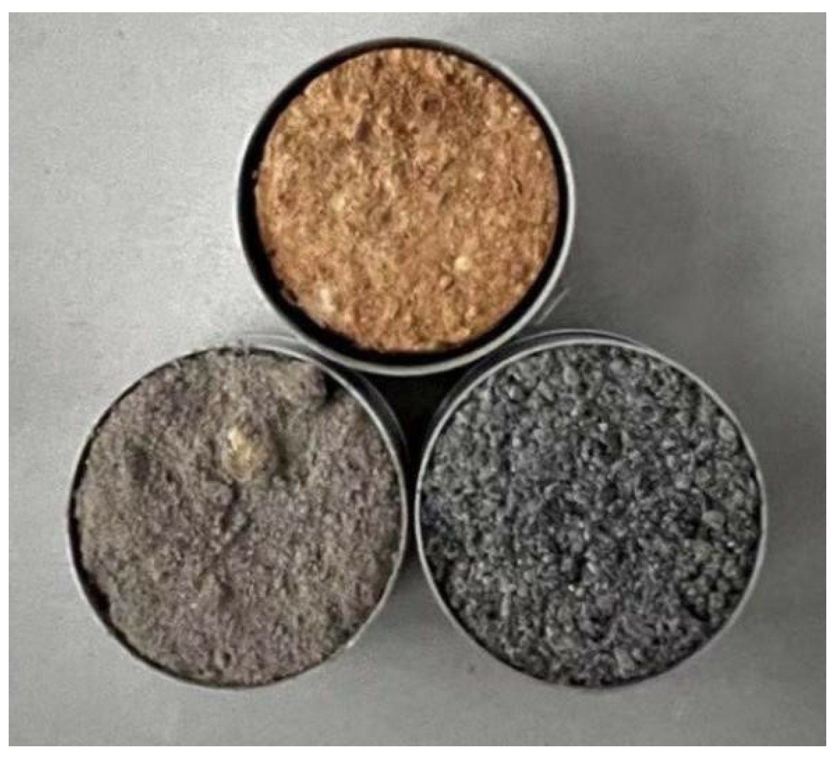
To ensure accuracy of the experiments, three soil medium were used in the present study (Figure 1). These medium included loamy soil, sandy loam and sand; they were all collected from Hangzhou, Zhejiang, China. An overview of the physical properties of the soils is given in Table 1 (herein, soil particle size is expressed as effective size ). All soil medium were excavated by excavators at the construction site; these soils were crushed into small particles for subsequent compaction and filling in the experimental setup.
During the experiments, the soil medium were kept completely dry to effectively calculate the diffusion coefficients of gas in soil. In addition, the three soil medium were sterilized and disinfected before the experiments to remove microorganisms that act as potential sources or sinks. The purpose of using dry soil is to exclude the interference of CO2 gas slightly soluble in water while moisture fills the pores in the soil to the experimental results, i.e., to control the soil moisture content to zero in order to facilitate the investigation of the effect of a single pressure decay wave on the gas flux at the soil surface.
2.5. Trace Gas
The trace gas used in the experiments included CO2 with a molar fraction of 2000 ppm, and the remaining part of the trace gas included air. In this study, trace gas was encapsulated in a compressed gas tank and injected into the experimental setup using a catheter. CO2 concentration was set at 2000 ppm for three main reasons: (1) the overall density of air does not vary much at this concentration [42]; (2) CO2 concentration of 2000 ppm is more consistent with the actual CO2 concentration at near-surface soil under natural conditions [43], and it is therefore representative of the natural conditions; and (3) it is a moderate concentration, and it is easier to reach steady state in the soil column in the experimental setup during actual aeration.
During the experiments, CO2 gas was injected into the bottom of the experimental apparatus at a slow and constant flow rate of 0.5 L·min−1 (Figure 2) before the experiment and diffused from the bottom to the top of the apparatus. When CO2 concentration reached steady state in soil column, then the gas tank was closed. All experiments were performed with sufficient CO2 gas in the gas tank.
2.6. Experimental Setup
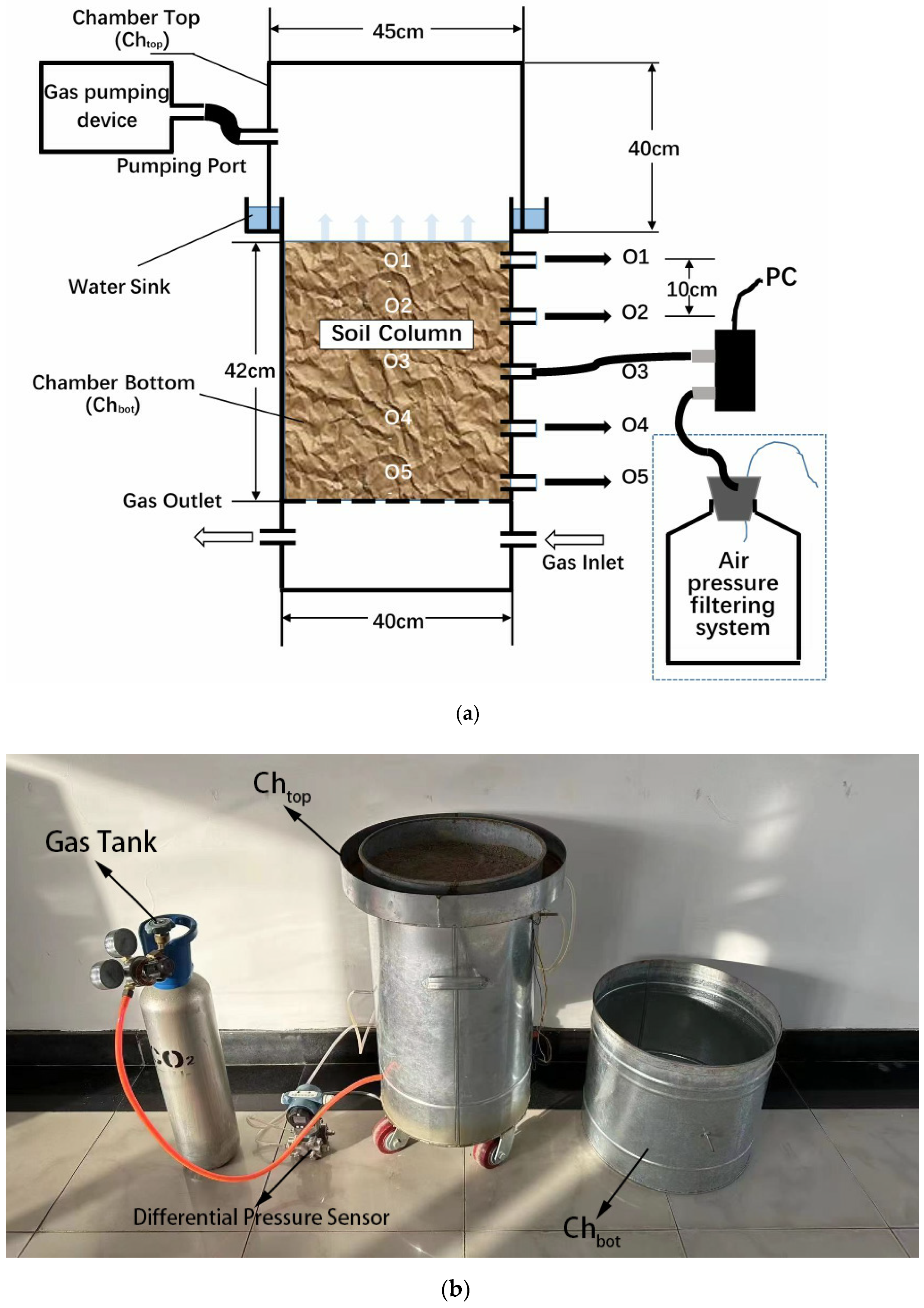
Figure 2 shows the overall layout of the experimental setup. The device was mainly composed of two parts—upper and lower—both made of stainless steel. The upper end consisted of a removable cylindrical gas chamber cover (Chtop) with a diameter of 45 cm and a height of 40 cm. The top surface of Chtop is closed, whereas its bottom surface is open. A conduit of 6 mm diameter was present on the side of the column as an induced pressure pump port, which could be connected to different pressure pump instruments. The gas pumping device used in this study included a self-made pressure pump, which consists of air cylinders and a box for storage. A cylindrical barrel (Chbot), which was 40 cm in diameter and 70 cm in height, was placed right below Chtop. The top surface of Chbot was open, whereas the bottom surface was closed. In Chbot, a 5 cm wide and 5 cm high upward ring water sink was welded at the side near top surface of Chbot to prevent the gas leakage between upper and lower parts of the interface in the experimental process. Moreover, in Chbot, gas tubes marked O1, O2, O3, O4, and O5 were installed at depths of 0 cm, 10 cm, 20 cm, 30 cm, and 40 cm from the top of the column, respectively. Below the O5 layer is a ventilation chamber, which is separated from Chbot by a perforated breathable screen and contain enough high concentration CO2 gas after the gas tank was closed to make sure that CO2 can supply for sufficient time(half an hour to one hour) during experiment. Four gas inlet and outlet tubes of 6 mm diameter are attached to the ventilation chamber (to facilitate ventilation and balance the pressure difference in the chamber; only two are marked in Figure 2).
Five CO2 concentration sensors (Beijing Dihui Technology Co. Ltd., Beijing, China), one in each layer between O1–O5 were placed in the soil. The sensor model DCO2-TFW1 has built-in NDIR infrared sensors (SenseAir, Delsbo, Sweden) and uses infrared principle to directly measure the CO2 molar fraction (ppm) of CO2-rich air, with data updated every 4 s. In the present study, molar fraction was used to characterize CO2 concentration. The pressure difference between soil column and the air outside the device as well as the pressure difference between layers at different depths within the soil column were monitored using a closed differential pressure transducer, model HCS3051 (Qingdao Huacheng Measurement and Control Equipment Co. Ltd., Qingdao, China). The differential pressure data was sampled every 0.5 s.
2.7. Pump Height
Different heights of pressure wave generation may lead to different nature of flow at the soil surface, and in order to find the appropriate height of pump arrangement, it needs to be analyzed in conjunction with the boundary layer theory. According to Figure 2, the pump draws or pumps gas into the interior of the experimental setup from the horizontal direction, and thus, different degrees of horizontal and vertical velocity components are generated inside the Chtop, and the closer the pump is to the soil surface, the larger is the horizontal velocity component. Meanwhile, the gas flow will produce shear force near the soil surface, so that part of the gas kinetic energy transfers to internal energy, resulting in a certain loss of kinetic energy, the part of the flow area affected by shear force is the boundary layer. It is reasonable to set the height of the pressure pump at a position larger than the thickness of the boundary layer.
To estimate the boundary layer thickness, firstly, it is necessary to determine whether the flow is laminar or turbulent, which can be determined by the Reynolds number. Assuming that all vertical component is converted to the horizontal velocity component, the Reynolds number can be defined as below:
The Reynolds number of the flow past the soil surface in Chtop can be calculated and determined whether it is laminar or turbulent. In Equation (10), is the gas density (kg·m−3), is the average flow velocity of the gas in the horizontal direction inside the device caused by the pump (m·s−1), is the characteristic length (m), which for this study is the diameter of the Chbot, is the aerodynamic viscosity (Pa·s), which is taken as 1.79 × 10⁻⁵ Pa·s. The assumption that the vertical velocity is fully converted to horizontal velocity can be approximated by the following equation:
where is the gas flow rate (m3·s−1) pumped or pumped into the interior of the device, and is the radius with Chbot (m). In this study, the maximum value of is taken not more than 0.5 L·s−1, so substituting it into Equations (10) and (11), the Reynolds number can be roughly calculated as 363, so most of the flow as a whole can be considered as laminar flow.
Thus, according to the literature [44], the thickness of the boundary layer (m) at laminar flow situation can be estimated as:
Taking as the diameter of Chbot, the thickness of the boundary layer is approximately 0.1 m. The conduit in Chtop is located at a height of 0.2 m from the bottom of the air chamber, so the height of the set pump meets the demand and does not cause violent turbulence fluctuations on the soil surface, which excludes the influence of complex air motion and facilitates the control of a single pressure wave for the experiment.
2.8. Experimental Protocol
The experiment aimed to analyze and quantify the effects of pressure fluctuations on gas transport in different soils, and to identify the physical properties of the soil that dominate gas transport in soil. In the experiment, air pressure fluctuations were created on the soil surface under controlled laboratory conditions (the room temperature of 25 °C and humidity of approximately 50% were maintained) The experimental protocol was divided into two parts to ensure rigor of the results: validation of the pressure decay model and response to CO2 concentration changes. First, the accuracy of the advection velocity, which was calculated using Equation (5), was established by studying the effect of pressure change on gas transport and validating the PAM model that establishes the pressure-gas emission relationship. Thereafter, an experiment was conducted to study the effect of pressure on CO2 gas concentration. Based on the results obtained from the experiments, the CO2 trace gas fluxes at the soil surface were calculated and compared with the fluxes obtained using closed chamber method for analysis.
2.8.1. PAM Model Validation
PAM model validation was divided into two main validation sessions: (i) the pattern of the variation in pressure difference between the O1–O5 layers (Figure 2) and the external reference cavity when the cylindrical barrel Chbot was filled with soil columns; and (ii) the decay curve of the pressure difference between the O1 layer (surface layer of the soil column) and O5 (bottom layer of the soil column) in Chbot with time was measured.
During the experiment, a self-made pressure pump was used to set pumping and pressing, and the actual amount of gas extracted from or pressed into the experimental setup was divided into five levels of 100 mL, 200 mL, 300 mL, 400 mL, and 500 mL, which were abbreviated as levels 1P, 2P, 3P, 4P, and 5P, respectively.
The experiment included the following steps (letters a and b in the step number indicate that the step corresponds to verification sessions (i) and (ii), respectively): (1) the soil was filled into the O1–O5 layer of Chbot; (2) the hollow side of Chtop was snapped onto the annular water sink of Chbot filled with soil (Figure 2), and water was added to the sink to prevent gas leakage during the experiment; (3) the low-pressure end (L) of the differential pressure sensor was connected to the lead pipe of the O1 layer in Chbot, with the rest of the layer closed and the high pressure end (H) was connected to the reference chamber (Mohr et al., 2020); (4) the pressure pump was connected to the pump port of Chtop, and air was pumped and pressurized in sequence from levels 1P to 5P into Chtop, and the initial peak differential pressure data was recorded each time; this step was repeated several times; (5) the pilot tube of O1 layer was sealed and the low pressure end (L) of the pressure sensor was connected to the pilot tubes of the O2, O3, O4, and O5 layers in turn (during this step, the other layers were sealed), and step (4) was repeated; (6) the low pressure end (L) and the high pressure end (H) of the differential pressure sensor were connected to the pilot tubes of the O1 layer O5 layer, respectively, and the conduit of the remaining layers was sealed; (7) the pressure pump was connected to the pump port of Chtop, the chamber was pumped and pressurized in the order of levels 1P–5P; the complete pressure difference decay curve between O1 layer and O5 layer was recorded each time, and the data was transferred to a computer. The experiment was repeated at least three times.
For the verification session (b), it was known that the radius of the Chbot was (m), the time of decay of the pressure difference was (s), the spacing between O1 and O5 layers was (m), and the pressure difference was calculated as . According to the PAM model, the theoretical pumping or pressurization volume was calculated from the experimental data using Equation (13):
where is the initial peak of the differential pressure decay curve. Equation (13) was used to compare with the actual volume of gas pumped or pressed by the pressure pump.
2.8.2. Concentration Change Response
The response of CO2 concentration within the soil column of different soil types to the pressure fluctuations created by the pressure pump was investigated. Moreover, the corresponding concentration data was collected to calculate the CO2 flux.
The experimental steps are listed below: (1) the CO2 concentration sensor was placed in the reference chamber for calibration before the experiment, Chtop was removed from Chbot, and the chamber was gradually filled with soil from O5 layer, and one concentration sensor was placed in each buried layer; (2) the top of the Chbot was opened, CO2-rich air (molar fraction concentration of 2000 ppm) was passed through the gas inlet conduit (Figure 2) into the gas chamber at the bottom of Chbot. The laboratory was kept open for ventilation, and the mole fraction of CO2 in the O1–O5 layers were recorded in real time using the CO2 concentration sensor. After a few hours of aeration, the CO2 gas concentration in the soil column inside the device leveled off and formed a nearly constant gradient between different layers; (3) Chtop was snapped smoothly above Chbot and the annular sink was filled with water to prevent air leakage, the concentration of CO2 on the soil surface at O1 layer at this stage was recorded and analyzed; (4) when all CO2 concentration sensors inside the Chbot readings were stable again, the pressure pump was connected to the pump port of the Chtop and the pumping and pressurization experiment was conducted; and (5) the CO2 concentration sensors located in the O1–O5 layers in Chbot were removed and placed in the reference chamber uniformly until stable concentration readings were recorded to ensure that no abnormal noise data occurred during the experiment.
After the above experimental steps, the CO2 flux on soil surface was calculated using the obtained CO2 molar fraction. The effect of pressure on the flux was evaluated by taking the ratio of the advection flux to the diffusion flux, as given below:
where is the CO2 concentration in the O1 layer (i.e., the soil surface); and can take the values 2, 3, 4, and 5 so that and represent the difference in pressure and concentration between the O1 layer and the O2, O3, O4, and O5 layers, respectively, in the experimental setup; and represent the depth between the O1 layer and the O2, O3, O4, and O5 layers of the soil.
It is worth noting that for the experimental step (3), the flux calculated using Equation (5) was further validated by using the flux measurement principle of confined gas chamber as Chbot was completely confined using Chtop.
The closed chamber method is widely used for measuring soil respiration, which involves placing a completely enclosed chamber on the soil surface and calculating the flux by measuring the CO2 gas concentration over time [45,46]. This method was similar to that used in the present study to investigate the emission of soil surface gases. The closed chamber method can be expressed as follows:
where is the difference in CO2 concentration at the O1 layer over time after the device was completely sealed, is the volume of gas covered by the cylindrical gas chamber lid Chtop (m3), is the radius of the cylindrical gas chamber lid Chtop (m), and is the remaining height of the Chtop after it was snapped into the sink (m).
3. Results
3.1. Model Reliability
The results of the model validation tests are discussed separately according to the validation sessions (i) and (ii) delineated in Section 2.8. For the validation session (i), the peak instantaneous pressure difference between each layer of soil column (O1–O5 layers) inside the Chbot and outside the experimental setup was recorded, and the peak pressure difference in all three soils showed a linear decreasing trend, and the linear fit was good (Figure 3a—it used the average data of pressure difference from multiple trials. It was demonstrated that the three soil media used in the experiment conformed to Darcy’s law, which suggests that the gas flow caused by pressure difference can be considered as Darcy’s flow, thereby indicating that the advection velocity that was calculated using Equation (5) is reliable.
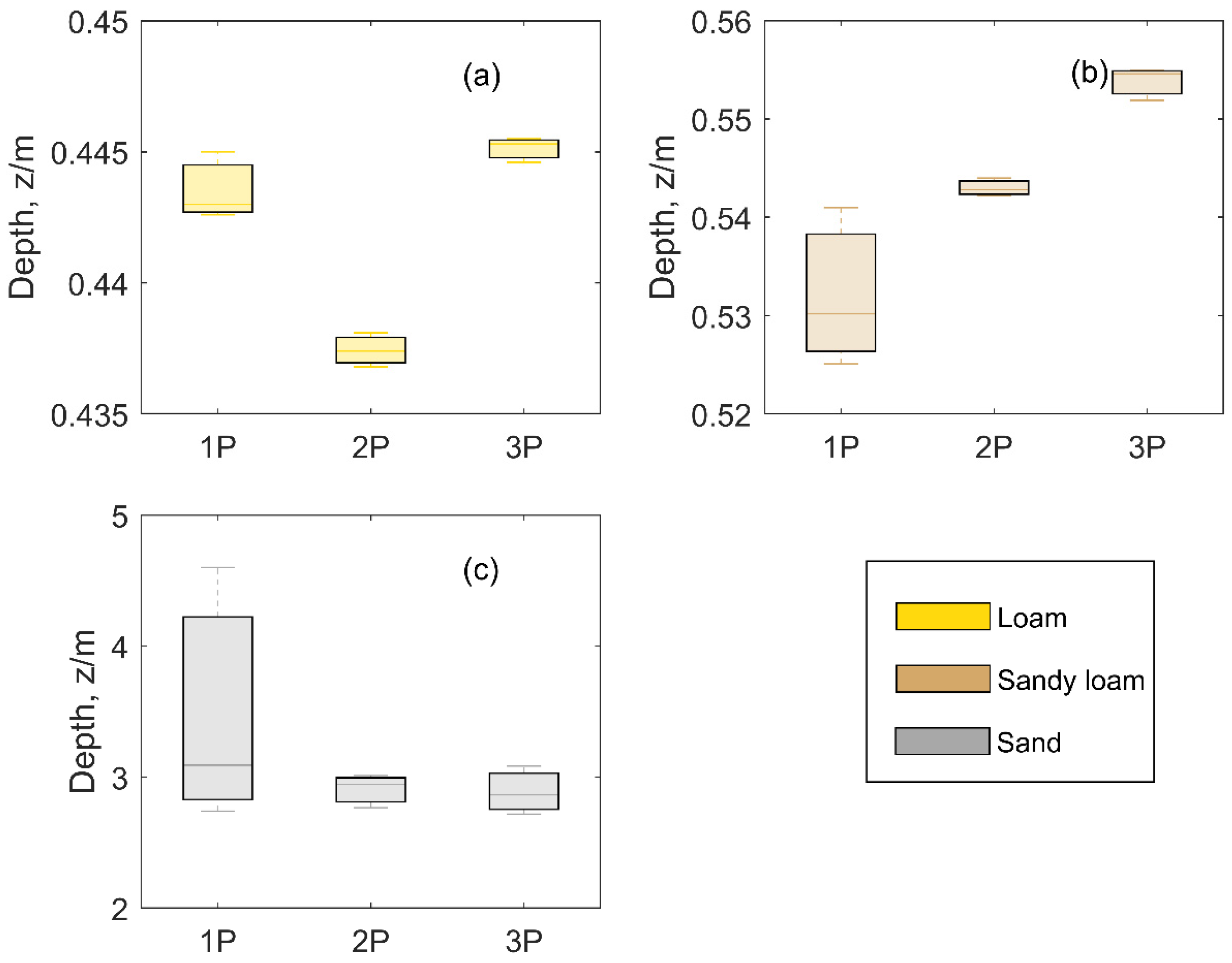
The results of the validation session (i) showed that for the same soil medium, the maximum distance depth (m) at which the pressure fluctuations can transmit their influence within the soil column in the Chbot is very similar, regardless of the pressure difference inside and outside the experimental setup Chbot (Figure 3b and Figure 4). It can be assumed that the maximum depth of the pressure difference has a certain value, which is only related to the physical properties of the soil, provided that the gas inside the experimental soil column is sufficient. This phenomenon has been analyzed in Section 3.3.
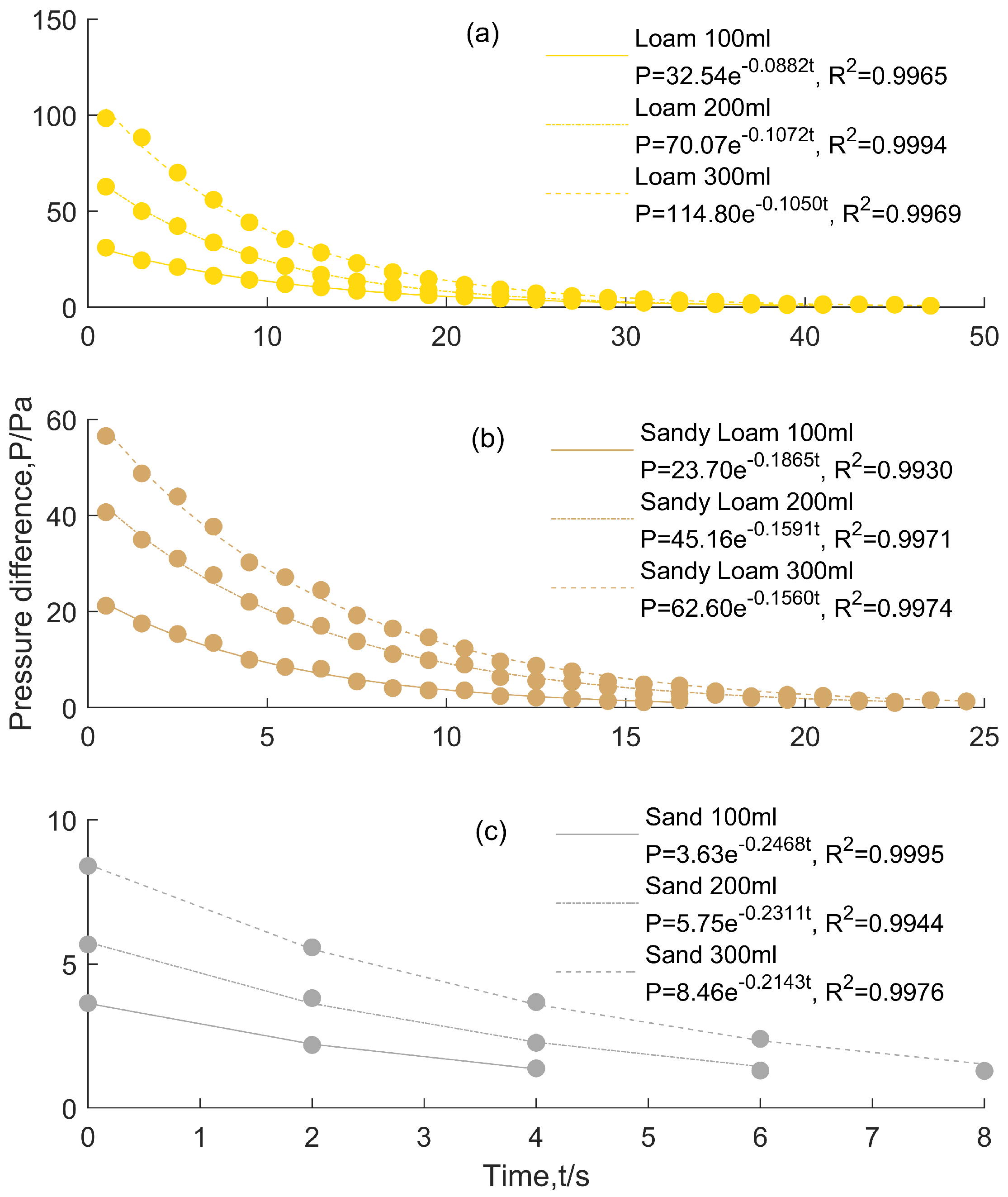
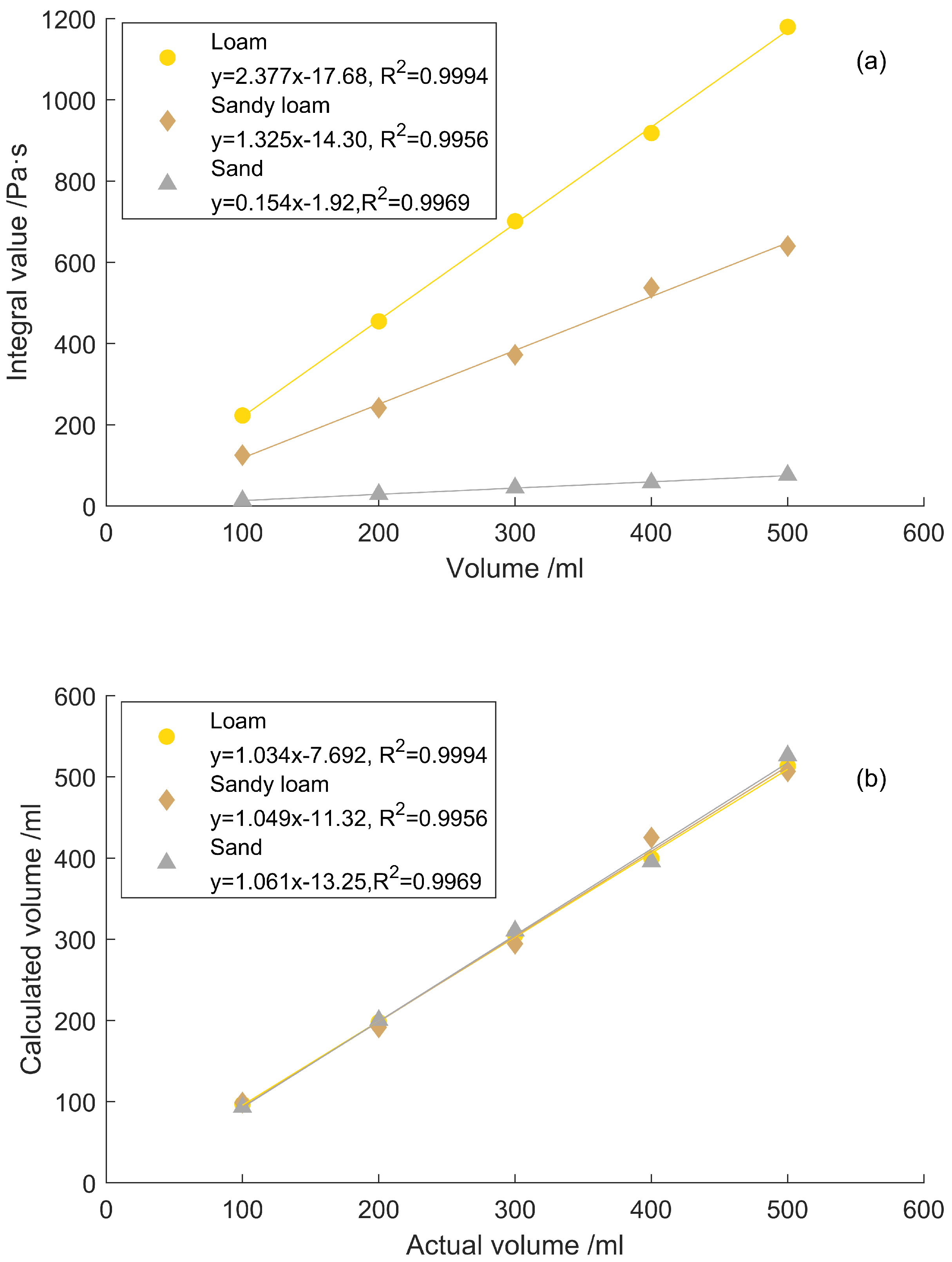
The results of the PAM model validation for validation session (ii) are shown in Figure 5. The pressure difference decay curves between the O1 and O5 layers in the three soil media conform to the exponential decay form described by Equation (8). Only cases corresponding to levels 1P–3P of pumping pressure have been plotted in Figure 5a–c. Based on the experimental data, the decay constant was fitted, and the fitted curve was integrated using Equation (9) to calculate the volume of gas that was transported in the experimental setup by the advection velocity. Theoretically, this volume of transported gas should be equal to the volume of gas extracted or pressed into the device by the pressure pump. Theoretical calculations and experimental data showed that the theoretical volume of transported gas for the three soils was almost similar to the actual volume of gas pumped (Figure 6b) and is proportional to the magnitude of the pressure difference (Figure 6a). Hence, PAM can be considered valid and reliable, and the results validate the accuracy of Equation (5), which can be used to calculate the advection velocity.
3.2. Calculation and Comparison of CO2 Response and Flux
The focus of the present study was to investigate the effect of pressure on the gas fluxes at the soil surface, and thus the CO2 concentration data at the soil surface were selected as the focus of the discussion of the study findings. Figure 7 shows a partial time series plot of the CO2 gas concentration changes at the O1 layer of the three soils, which corresponds to the experimental step (3) in Section 2.8.2. This plot represents the pattern of CO2 molar fraction changes at the O1 layer of the soil surface after Chtop was capped to Chbot, thereby completely sealing the chamber. In the plot, time period I (0–50 s) indicates the state after the CO2-rich air was continuously introduced at the inlet in Chbot (Figure 2) before Chtop was covered and the CO2 molar fraction of the O1 layer reached steady state; time period II (50–100 s) shows the molar fraction distribution of CO2 at O1 layer of the soil column after Chtop was covered during the aeration state; time period III (after 100 s), 500 mL of gas was extracted in the gas chamber using the pressure pump, and the CO2 molar fraction at the O1 layer was changed accordingly.
During period II, the CO2 molar fraction at the O1 layer of sand increased at a fast rate, which can likely be attributed to the much larger soil particle size and soil gas permeability of sand compared with the other two soils, making it easier for the high molar fraction of CO2-rich gas to diffuse to the soil surface in the soil column when filled with sand. For time period III, the CO2 molar fraction at O1 changed similarly for all three soils after 500 mL of air was pumped, but even in this case, sand showed most clear changes. Combining this observation with Equation (5) (Darcy’s formula), it is known that the higher permeability of sand (nearly 10 times larger than loam and sand) increases the advection velocity that is generated by the pressure difference after pumping. This increases the molar fraction of CO2 in the air near the O1 layer after 140 s (Figure 7) and decreases it after 140 s. The reason is that the advection velocity gradually decreases as the pressure difference decays. Meanwhile, from the perspective of Equation (1) (ADE), the right side of Equation (1) contains the term III determined by the advection velocity, and the term I on the left side of Equation (1) changes with the advection velocity while the term II is approximately constant, which further supports the phenomenon of CO2 molar fraction change.
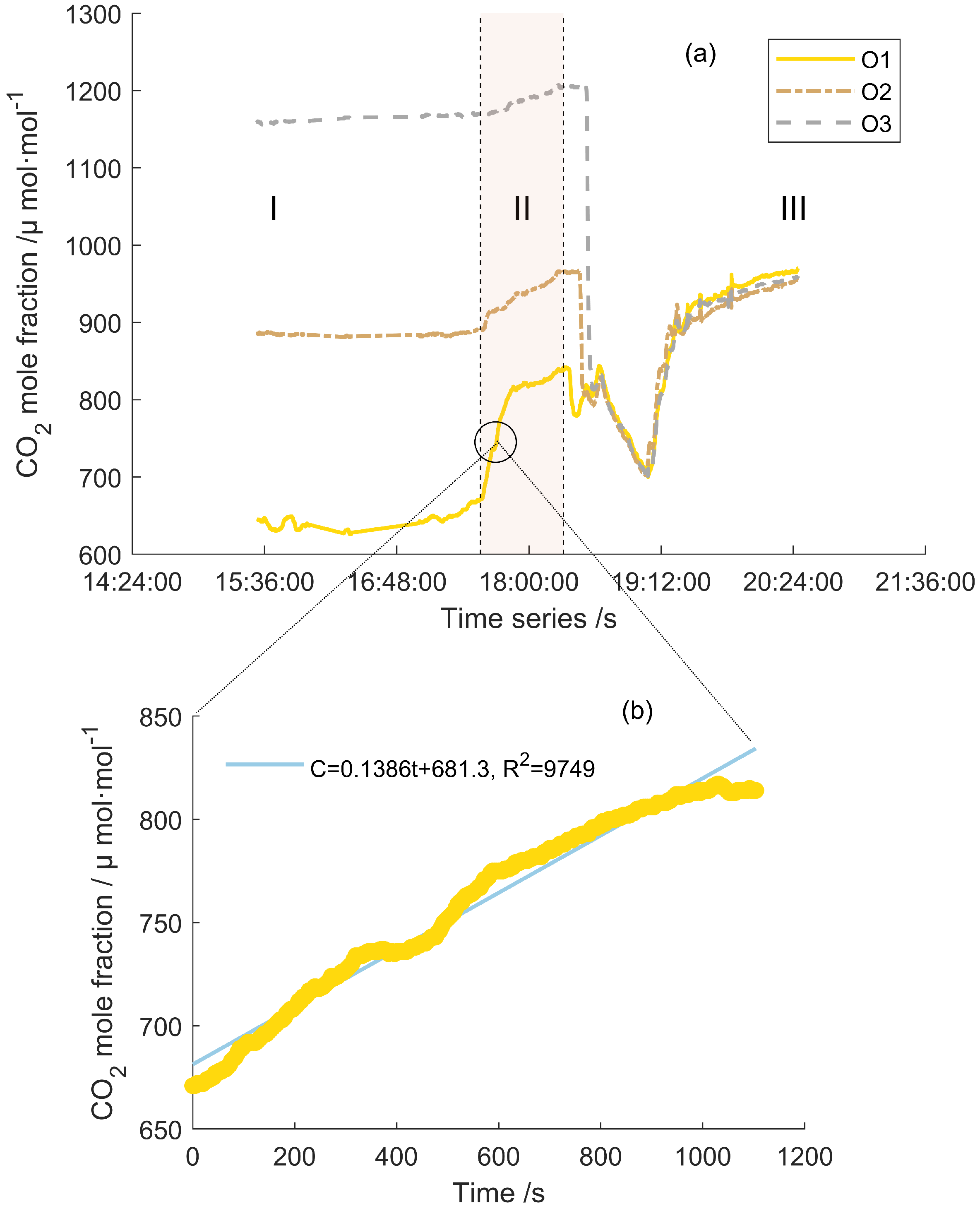
Thereafter, CO2 fluxes on the soil surface were calculated. As an example, the experimental results of only sandy loam are discussed here, (the experimental phenomena were similar for the remaining two media). Figure 8 shows the variation of CO2 concentration in the O1–O3 layers of the sandy loam in Chbot from the afternoon to the night of 13 June 2021. In the figure, the experimental data has been divided into three stages. Stage I (15:32–17:13): after continuous aeration in the soil column, the CO2 molar fraction of the O1–O3 layers reached a plateau (the concentration gradient between layers was almost constant). Stage II (17:13–18:18): Chtop was covered and no changes were made until relative stabilization of CO2 molar fraction of the O1–O3 layers was achieved. After the relative stabilization, 100 mL of gas was continuously pumped, beginning at approximately 17:33 for approximately 17 min. Stage III (after 18:18): Chtop was removed and the concentration sensors were moved from the soil column inside the Chbot to the reference chamber.
The mechanism of gas transport during the stage I included only diffusion, which converted the average molar fraction gradient between the O1 and O2 layers and the O2 and O3 layers (Figure 8a; O4 and O5 layers are not shown in the figure) into a molar concentration gradient that could be calculated using Equation (2) for pure diffusion flux on the soil surface of the O1 layer at steady state.
During stage II, the approximate linear model of the molar concentration change at O1 can be expressed using Equation (16):
Fitting the data for 17:33–17:52 period, was calculated as 0.14 (Figure 8b). The values 24.5 and 103 in the above equation converts the molar fraction into molar concentration so that the value of is obtained. By substituting this value in Equation (15), the calculated CO2 flux value was calculated as 2.23 μmol·m−2·s−1, which was used as a reference value for comparison.
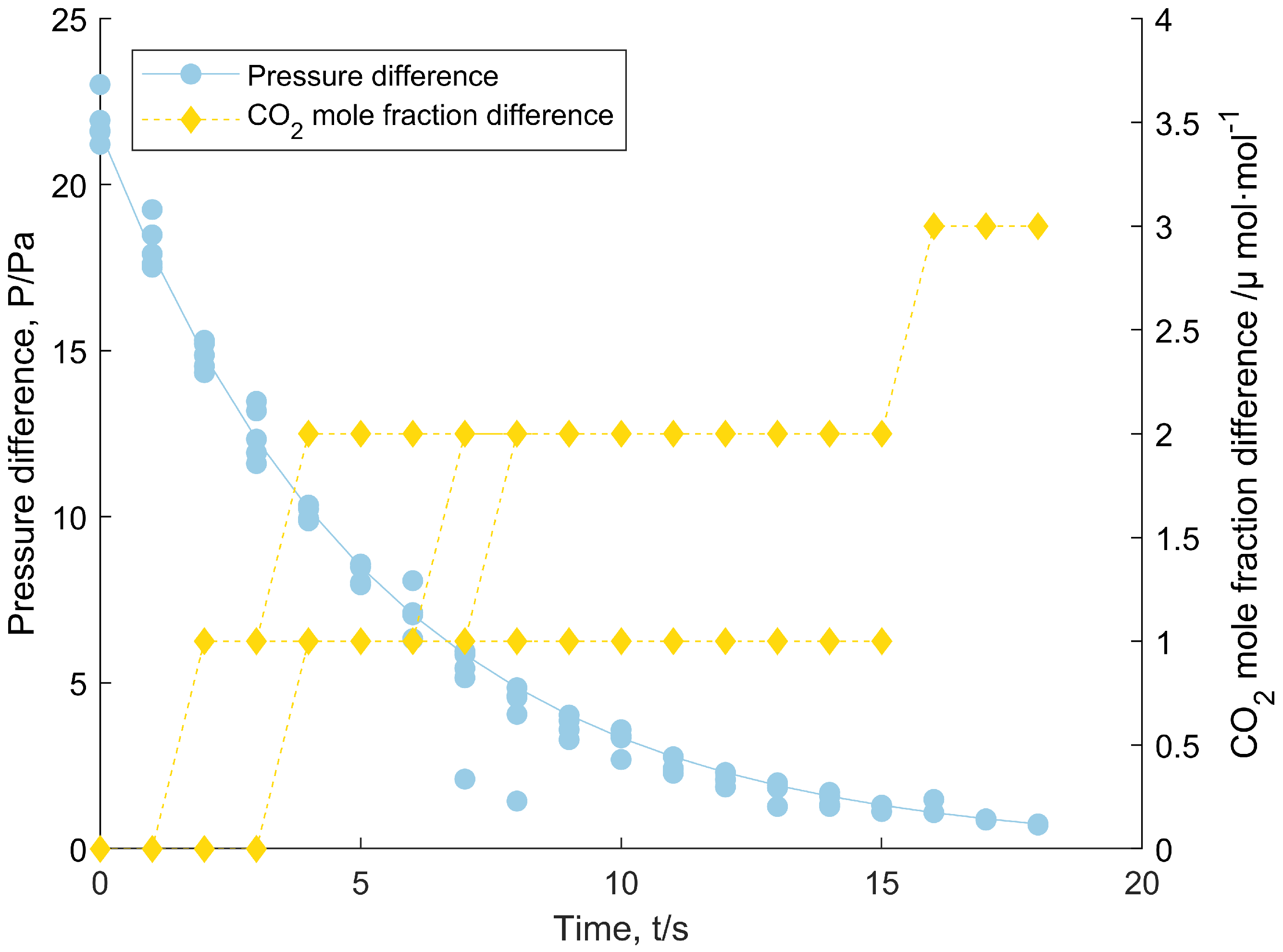
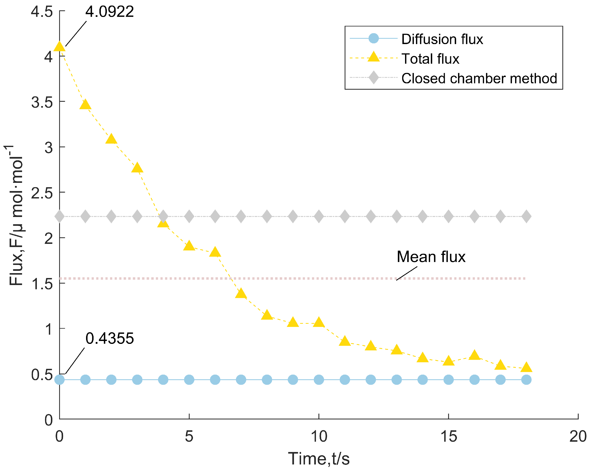
The effect of the pressure difference on the flux at the soil surface O1 was calculated using the total flux form expressed in Equation (6). This was added as to the original diffusion flux. In stage II, the decay of the pressure difference between the O1 and O5 layers of the sandy loam and the variation pattern of the CO2 mole fraction at the O1 layer are shown in Figure 9. The values of the variation of the CO2 mole fraction at the O1 layer were similar to the fraction after the decay of the pressure difference was completed. The calculation shows that the maximum instantaneous total flux determined by the peak pressure difference is approximately 4 μmol·m−2·s−1 when the negative pressure of approximately 21 Pa still exists at the soil surface (Figure 10), which is larger than the flux calculated using Equation (15). This is likely because the flux value calculated by Equation (15) represents the average flux throughout the pumping stage. After averaging the flux calculated by Equation (6), it was found that the flux calculated using Equation (15) was more consistent.
Finally, the effect of the pressure difference on the CO2 flux at the soil surface was evaluated using Equation (14). It was observed that pressure pump enhanced the flux. For stage II, the concentration gradient between the O1 and O2 layers at the first pumping pressure (Figure 8) and the pressure difference between the O1 and O5 layers (Figure 9) were used to calculate the diffusion and advection fluxes. These fluxes were then combined with Equation (14) (taking , ) to measure the real-time enhancement effect. Figure 10 shows that a pressure difference of approximately 21 Pa between the soil surface and the bottom of the soil column resulted in a great increase in the total flux at the soil surface by a factor of approximately 8.4 compared to the steady state (pure diffusion). Similar calculations were performed for the other two soil media, and according to the experimental data, the fluxes on the surfaces of loam, sand, and sand increased by approximately 0.61, 1.59, and 13.1 times for each 1 Pa of negative pressure generated between the O1 and O2 layers when , , respectively (specific data not given in this paper). This indicates that changes in pressure greatly affect gas emissions from the surfaces of various soil media.
3.3. Response of Soil Physical Properties to Pressure Difference
In the present study, two phenomena were observed: (i) for the same soil species, the maximum soil depth that can be affected by the pressure difference is a specific value, irrespective of the magnitude of the positive or negative pressure difference created on the soil surface by the pressure pump; (ii) for different soil species, when the same volume of gas was pumped or pressed into the experimental apparatus, a variation in the peak initial pressure difference was generated.
Therefore, for different soils, the relationship between the maximum affected depth and the initial peak of the pressure differential effect of the above properties was measured by combining the particle size, air permeability, total porosity of the soil, (Table 1) and the ratio between the two different properties. The results of the present study suggested that the maximum depth of the pressure difference transfer was positively correlated with soil permeability. Furthermore, the absolute value of the peak value during pressure pumping and pressurization was negatively correlated with particle size and soil permeability, whereas total porosity were not highly correlated with maximum distance and peak pressure difference (Figure 11). Soil permeability was identified as the key physical property that affects the sensitivity of the soil medium to pressure. In the present study, the rank of sensitivity among three soils was sand > sandy loam > loamy soil.
From the above results and the experimental results in Section 3.1, it can be concluded that soil gas permeability is the key physical property that determines the sensitivity of the soil medium to changes in pressure difference response.
4. Discussion
Though the present study verified that the PAM model can reliably describe the soil gas emission and pressure variation, it focused on the results of the variation of CO2 flux on the surface of sandy loams. A change in air pressure of 1 Pa at the surface of sandy loams results in approximately 2.5 times greater gas flux than that of a pure diffusion process. This observation is similar to that reported by Bain, Hutyra, Patterson, Bright, Daube, Munger and Wofsy [32], Xu, Furtaw, Madsen, Garcia, Anderson and McDermitt [33]. These researchers have reported that pressure fluctuation of approximately 2.4 Pa increases flux by 2.33 times. The experimental study of monotonic pressure decay waves in this study suggested that if pressure fluctuation is similar to a sinusoidal wave at the soil surface, the total gas emission (in this paper, CO2-rich air) can be considered as balanced (i.e., the volumes of gas entering and exiting at the soil surface should be equal). However, when calculating the emission or gas flux for a component gas (CO2 in this study), the concentration of the component gas needs to be further considered to calculate the flux precisely. Moreover, the actual calculation should also consider the gas entering the soil as a negative direction (when the soil is considered a sink), the gas leaving the soil as a positive direction (when the soil is considered a source), and the effect of pressure on the gas emissions from the soil surface as a result of the two separate calculations should be evaluated. The concentration of CO2 in soil (up to 13% in near-surface soils) is several times greater than that in air [47], and the probability of soil functioning as a source is relatively high when a sine wave-like pressure variation occurs at the soil surface (i.e., the total cumulative CO2 emissions from the soil surface are still increasing under the effect of sinusoidal pressure fluctuations). For natural soils in field, the proportion of O2 (Oxygen) in air is greater than that in soil. Hence, sinusoidal pressure changes may be more conducive to O2 exchange into the soil interior, making it easier for some soil microorganisms and roots to respire and enhancing the biological activity of the soil.
In addition, when combining the results of this study with the soil CO2 fluxes in field, which is measured using the closed chamber method, it is necessary to consider the influence pressure difference between the outside and inside of the gas chamber. In this case, an equilibrium pressure difference treatment for the gas chamber should be adopted to reduce the measurement error. Two main factors are considered to affect the pressure inside and outside the chamber [33], which are listed below: (i) temperature changes or water vapor release inside the chamber; and (ii) the wind outside the chamber during the actual measurement. A temperature deviation of 1 °C inside the gas chamber will result in a pressure change of 333 Pa. The release of water vapor causes a positive pressure inside the chamber, which inhibits the emission of gases from soil surface. If surface winds occur in the vicinity of the area where flux is being measured using the closed chamber, the pressure inside the chamber will deviate from that outside, resulting in under- or overestimation of CO2 fluxes.
5. Conclusions
This study focused on the effect of barometric pressure fluctuations (represented in the form of attenuation waves) on gas emissions from the soil surface. Additionally, it verified the relationship between pressure differences and gas emissions from the soil surface using a derived PAM model. The study also quantified the effect of pressure differences on gas fluxes, which may vary by orders of 1 Pa increase of 100%. The study used three real soil media collected from the field and focused on exploring the less studied attenuation waves, repeating the experiment several times to ensure that the findings are representative. In addition, this experimental study found that in any kind of soil that is uniformly distributed and consistent with Darcy flow, the pressure difference generated at the soil surface varies linearly with depth. In soil that is subjected to barometric pressure fluctuations, the instantaneous depth of influence of the pressure difference is related only to the physical properties of the soil (i.e., any size change in pressure affects the same soil medium to the same depth); this is true if the total volume of internal gas is much larger than the volume of gas required to change the equilibrium pressure difference. The sensitivity of the gas response to pressure changes in soil media is positively correlated with the gas permeability in the soil. The gas permeability of soil is a key physical property that affects the gas emission from the soil surface. For sandy loams, a pressure change of 21 Pa between soil surface and bottom produces an instantaneous CO2 flux 9.396 times greater than that in the steady state (pure diffusion). With relatively uniform soil gas concentrations, the effect of the same 1 Pa pressure variation on surface gas fluxes follows the given trend: fine sand > sandy loam > loamy soil.
However, there were a few limitations with the present study: (i) the dispersion effect was not considered, which may influence soil surface gas transport; (ii) soil medium were dried and sterilized, which is not representative of natural soil conditions; (iii) only CO2 was explored as trace gas, whereas other GHGs, such as N2O and CH4, were not considered.
The study findings provide a theoretical basis for assessing the effects of other environmental factors on soil surface gas flux in field. The model proposed in the present study will be validated in the field in future studies. Furthermore, it will be combined with other factors that influence emissions to ensure an integrated analysis. For example, wind and temperature-driven convective transport mechanisms can be further investigated as a complex mix of pressure changes and gas shear effects in the influence of winds are present. Moreover, temperature changes also occur in response to changes in air pressure and other factors. Hence, further investigations on the effects of pressure would be essential. Nonetheless, the findings of simple decay waves that are mentioned in the present paper can provide a strong basis for future complex studies.
Author Contributions
Conceptualization, J.J., K.G. and J.X.; methodology, J.J., K.G. and J.X.; software, K.G., Y.L. (Yao Li) and Y.L. (Yang Le); validation, J.J. and K.G.; formal analysis, J.J. and K.G.; investigation, J.J. and K.G.; resources, J.J. and J.H.; data curation, J.J., K.G., Y.L. (Yao Li) and Y.L. (Yang Le); writing—original draft preparation, J.J. and K.G.; writing—review and editing, J.J. and K.G.; visualization, K.G.; supervision, J.X. and J.H.; project administration, J.H.; funding acquisition, J.H. All authors have read and agreed to the published version of the manuscript.
Funding
This research was funded by the National Natural Science Foundation of China (Grant Nos. 31971493 and 31570629).
Data Availability Statement
The data presented in this study are available in figures and tables provided in the manuscript.
Acknowledgments
The authors extend great gratitude to the anonymous reviewers and editors for their helpful reviews and critical comments.
Conflicts of Interest
The authors declare no conflict of interest.
References
- Forde, O.N.; Cahill, A.G.; Beckie, R.D.; Mayer, K.U. Barometric-pumping controls fugitive gas emissions from a vadose zone natural gas release. Sci. Rep. 2019, 9, 14080. [Google Scholar] [CrossRef] [PubMed] [Green Version]
- Hutchinson, G.L.; Livingston, G.P.; Healy, R.W.; Striegl, R.G. Chamber measurement of surface-atmosphere trace gas exchange: Numerical evaluation of dependence on soil, interfacial layer, and source/sink properties. J. Geophys. Res. Atmos. 2000, 105, 8865–8875. [Google Scholar] [CrossRef]
- Knorr, W.; Prentice, I.C.; House, J.I.; Holland, E.A. Long-term sensitivity of soil carbon turnover to warming. Nature 2005, 433, 298–301. [Google Scholar] [CrossRef] [PubMed]
- Sahoo, B.K.; Mayya, Y.S. Two dimensional diffusion theory of trace gas emission into soil chambers for flux measurements. Agric. For. Meteorol. 2010, 150, 1211–1224. [Google Scholar] [CrossRef]
- Hamamoto, S.; Moldrup, P.; Kawamoto, K.; Komatsu, T. Effect of Particle Size and Soil Compaction on Gas Transport Parameters in Variably Saturated, Sandy Soils. Vadose Zone J. 2009, 8, 986–995. [Google Scholar] [CrossRef] [Green Version]
- Kuang, X.; Jiao, J.J.; Li, H. Review on airflow in unsaturated zones induced by natural forcings. Water Resour. Res. 2013, 49, 6137–6165. [Google Scholar] [CrossRef]
- Levintal, E.; Dragila, M.I.; Weisbrod, N. Impact of wind speed and soil permeability on aeration time in the upper vadose zone. Agric. For. Meteorol. 2019, 269–270, 294–304. [Google Scholar] [CrossRef]
- Kristensen, A.H.; Thorbjørn, A.; Jensen, M.P.; Pedersen, M.; Moldrup, P. Gas-phase diffusivity and tortuosity of structured soils. J. Contam. Hydrol. 2010, 115, 26–33. [Google Scholar] [CrossRef]
- Costanza-Robinson, M.S.; Brusseau, M.L. Gas phase advection and dispersion in unsaturated porous media. Water Resour. Res. 2002, 38, 7–1–7–9. [Google Scholar] [CrossRef]
- Nield, D.A.; Bejan, A. Convection in Porous Media; Springer: Cham, Switzerland, 2006; Volume 3. [Google Scholar]
- Ganot, Y.; Dragila, M.I.; Weisbrod, N. Impact of thermal convection on CO2 flux across the earth–atmosphere boundary in high-permeability soils. Agric. For. Meteorol. 2014, 184, 12–24. [Google Scholar] [CrossRef]
- Kamai, T.; Weisbrod, N.; Dragila, M.I. Impact of ambient temperature on evaporation from surface-exposed fractures. Water Resour. Res. 2009, 45, W02417. [Google Scholar] [CrossRef]
- Lahmira, B.; Lefebvre, R.; Hockley, D.; Phillip, M. Atmospheric Controls on Gas Flow Directions in a Waste Rock Dump. Vadose Zone J. 2014, 13, 1–17. [Google Scholar] [CrossRef]
- Nachshon, U.; Weisbrod, N.; Dragila, M.I. Quantifying Air Convection through Surface-Exposed Fractures: A Laboratory Study. Vadose Zone J. 2008, 7, 948–956. [Google Scholar] [CrossRef]
- Nield, D.; Kuznetsov, A.V. An historical and topical note on convection in porous media. J. Heat Transf. 2013, 135, 061201. [Google Scholar] [CrossRef]
- Weisbrod, N.; Dragila, M.I.; Nachshon, U.; Pillersdorf, M. Falling through the cracks: The role of fractures in Earth-atmosphere gas exchange. Geophys. Res. Lett. 2009, 36, L02401. [Google Scholar] [CrossRef]
- Kimball, B.A.; Lemon, E.R. Air Turbulence Effects upon Soil Gas Exchange. Soil Sci. Soc. Am. J. 1971, 35, 16–21. [Google Scholar] [CrossRef]
- Nachshon, U.; Dragila, M.; Weisbrod, N. From atmospheric winds to fracture ventilation: Cause and effect. J. Geophys. Res. Biogeosci. 2012, 117, G02016. [Google Scholar] [CrossRef] [Green Version]
- Pourbakhtiar, A.; Poulsen, T.G.; Faghihinia, M.; Papadikis, K.; Wilkinson, S. Relating wind-induced gas transport in porous media to wind speed and medium characteristics. J. Pet. Sci. Eng. 2020, 194, 107550. [Google Scholar] [CrossRef]
- Pourbakhtiar, A.; Poulsen, T.G.; Wilkinson, S.; Bridge, J.W. Effect of wind turbulence on gas transport in porous media: Experimental method and preliminary results. Eur. J. Soil Sci. 2017, 68, 48–56. [Google Scholar] [CrossRef] [Green Version]
- Sánchez-Cañete, E.P.; Oyonarte, C.; Serrano-Ortiz, P.; Curiel Yuste, J.; Pérez-Priego, O.; Domingo, F.; Kowalski, A.S. Winds induce CO2 exchange with the atmosphere and vadose zone transport in a karstic ecosystem. J. Geophys. Res. Biogeosci. 2016, 121, 2049–2063. [Google Scholar] [CrossRef]
- Clements, W.E.; Wilkening, M.H. Atmospheric pressure effects on 222Rn transport across the Earth-air interface. J. Geophys. Res. 1974, 79, 5025–5029. [Google Scholar] [CrossRef]
- Massmann, J.; Farrier, D.F. Effects of atmospheric pressures on gas transport in the vadose zone. Water Resour. Res. 1992, 28, 777–791. [Google Scholar] [CrossRef]
- Sánchez-Cañete, E.P.; Kowalski, A.S.; Serrano-Ortiz, P.; Pérez-Priego, O.; Domingo, F. Deep CO2 soil inhalation/exhalation induced by synoptic pressure changes and atmospheric tides in a carbonated semiarid steppe. Biogeosciences 2013, 10, 6591–6600. [Google Scholar] [CrossRef] [Green Version]
- Hinton, E.M.; Woods, A.W. Shear dispersion in a porous medium. Part 1. An intrusion with a steady shape. J. Fluid Mech. 2020, 899, A38. [Google Scholar] [CrossRef]
- Webster, I.T.; Taylor, J.H. Rotational dispersion in porous media due to fluctuating flows. Water Resour. Res. 1992, 28, 109–119. [Google Scholar] [CrossRef]
- Alzaydi, A.A.; Moore, C.A.; Rai, I.S. Combined pressure and diffusional transition region flow of gases in porous media. AIChE J. 1978, 24, 35–43. [Google Scholar] [CrossRef]
- Bowling, D.R.; Massman, W.J. Persistent wind-induced enhancement of diffusive CO2 transport in a mountain forest snowpack. J. Geophys. Res. Biogeosci. 2011, 116, G04006. [Google Scholar] [CrossRef]
- Maier, M.; Schack-Kirchner, H.; Aubinet, M.; Goffin, S.; Longdoz, B.; Parent, F. Turbulence Effect on Gas Transport in Three Contrasting Forest Soils. Soil Sci. Soc. Am. J. 2012, 76, 1518–1528. [Google Scholar] [CrossRef] [Green Version]
- Poulsen, T.G.; Møldrup, P. Evaluating effects of wind-induced pressure fluctuations on soil-atmosphere gas exchange at a landfill using stochastic modelling. Waste Manag. Res. 2006, 24, 473–481. [Google Scholar] [CrossRef]
- Mohr, M.; Laemmel, T.; Maier, M.; Schindler, D. Analysis of Air Pressure Fluctuations and Topsoil Gas Concentrations within a Scots Pine Forest. Atmosphere 2016, 7, 125. [Google Scholar] [CrossRef]
- Bain, W.G.; Hutyra, L.; Patterson, D.C.; Bright, A.V.; Daube, B.C.; Munger, J.W.; Wofsy, S.C. Wind-induced error in the measurement of soil respiration using closed dynamic chambers. Agric. For. Meteorol. 2005, 131, 225–232. [Google Scholar] [CrossRef]
- Xu, L.; Furtaw, M.D.; Madsen, R.A.; Garcia, R.L.; Anderson, D.J.; McDermitt, D.K. On maintaining pressure equilibrium between a soil CO2 flux chamber and the ambient air. J. Geophys. Res. Atmos. 2006, 111, D08S10. [Google Scholar] [CrossRef] [Green Version]
- Takle, E.S.; Massman, W.J.; Brandle, J.R.; Schmidt, R.A.; Zhou, X.; Litvina, I.V.; Garcia, R.; Doyle, G.; Rice, C.W. Influence of high-frequency ambient pressure pumping on carbon dioxide efflux from soil. Agric. For. Meteorol. 2004, 124, 193–206. [Google Scholar] [CrossRef]
- Laemmel, T.; Mohr, M.; Schack-Kirchner, H.; Schindler, D.; Maier, M. 1D Air Pressure Fluctuations Cannot Fully Explain the Natural Pressure-Pumping Effect on Soil Gas Transport. Soil Sci. Soc. Am. J. 2019, 83, 1044–1053. [Google Scholar] [CrossRef]
- Poulsen, T.G.; Sharma, P. Apparent Porous Media Gas Dispersion in Response to Rapid Pressure Fluctuations. Soil Sci. 2011, 176, 635–641. [Google Scholar] [CrossRef]
- Scooter, D.R.; Thurtell, G.W.; Raats, P.A.C. NOTE: Dispersion Resulting from Sinusoidal Gas Flow in Porous Materials. Soil Sci. 1967, 104, 306–308. [Google Scholar] [CrossRef]
- Scotter, D.R.; Raats, P.A.C. Dispersion in Porous Mediums Due to Oscillating Flow. Water Resour. Res. 1968, 4, 1201–1206. [Google Scholar] [CrossRef]
- Millington, R.J.; Quirk, J.P. Permeability of porous solids. Trans. Faraday Soc. 1961, 57, 1200–1207. [Google Scholar] [CrossRef]
- Schery, S.D.; Gaeddert, D.H.; Wilkening, M.H. Factors affecting exhalation of radon from a gravelly sandy loam. J. Geophys. Res. Atmos. 1984, 89, 7299–7309. [Google Scholar] [CrossRef]
- Bear, J. Dynamics of Fluids in Porous Media; Courier Corporation: Chelmsford, MA, USA, 1988. [Google Scholar]
- Kowalski, A.S.; Sánchez-Cañete, E.P. A New Definition of the Virtual Temperature, Valid for the Atmosphere and the CO2-Rich Air of the Vadose Zone. J. Appl. Meteorol. Climatol. 2010, 49, 1692–1695. [Google Scholar] [CrossRef]
- Angert, A.; Yakir, D.; Rodeghiero, M.; Preisler, Y.; Davidson, E.A.; Weiner, T. Using O2 to study the relationships between soil CO2 efflux and soil respiration. Biogeosciences 2015, 12, 2089–2099. [Google Scholar] [CrossRef] [Green Version]
- Schlichting, H.; Kestin, J. Boundary Layer Theory; Springer: Berlin/Heidelberg, Germany, 1961; Volume 121. [Google Scholar]
- Bekku, Y.; Koizumi, H.; Nakadai, T.; Iwaki, H. Measurement of soil respiration using closed chamber method: An IRGA technique. Ecol. Res. 1995, 10, 369–373. [Google Scholar] [CrossRef]
- Rochette, P.; Hutchinson, G.L. Measurement of soil respiration in situ: Chamber techniques. In Micrometeorology in Agricultural Systems; American Society of Agronomy: Madison, WI, USA, 2005; pp. 247–286. [Google Scholar]
- Amundson, R.G.; Davidson, E.A. Carbon dioxide and nitrogenous gases in the soil atmosphere. J. Geochem. Explor. 1990, 38, 13–41. [Google Scholar] [CrossRef]
Figure 1.
Three different soil porous media that are uniformly placed in a circular bowl. The soil samples were exposed to an air-dried environment and used to measure total soil porosity.
Figure 1.
Three different soil porous media that are uniformly placed in a circular bowl. The soil samples were exposed to an air-dried environment and used to measure total soil porosity.

Figure 2.
(a) Illustration of self-designed gas chamber that is connected with other experimental instruments. The pumping port of the removable cylindrical gas chamber cover (Chtop) is connected to an external pressure pump, and the outer tube extending from O1 to O5 layers inside the lower bottom closed cylindrical barrel (Chbot) can be connected to one end of the differential pressure transducer, and the other end of the differential pressure sensor is connected to the reference chamber (air pressure filtering system, see the dashed box in the figure), which transmits CO2 by venting to the inlet port of the Chbot, and the outlet port is used to balance the pressure difference caused by the ventilation. Data collected from pressure transducer were transferred to PC (i.e., personal computer). (b) Physical diagram of the experimental setup, from left to right, are gas tank, differential pressure sensor, Chbot and Chtop, respectively, gas pumping device and PC are excluded.

Figure 3.
(a) Relationship between the pressure difference in the porous medium of the three soils and the depth of transmission (b) Propagation depth of the pressure in the three soils in the case of pumping 100 mL, 200 mL and 300 mL, the pressure difference caused by 1P-100 mL, the pressure difference formed by 2P-200 mL and the pressure difference formed by 3P-300 mL.

Figure 4.
Maximum depth in the medium that can be affected by the pressure difference of three different soils: (a) loam; (b) sandy loam; (c) sand, where 1P represents 1 first level (100 mL) of pressure difference, 2P, 3P, and so on.
Figure 4.
Maximum depth in the medium that can be affected by the pressure difference of three different soils: (a) loam; (b) sandy loam; (c) sand, where 1P represents 1 first level (100 mL) of pressure difference, 2P, 3P, and so on.

Figure 5.
Pressure decay curves for three different soil porous media: (a) Loam, (b) Sandy loam, and (c) Sand.
Figure 5.
Pressure decay curves for three different soil porous media: (a) Loam, (b) Sandy loam, and (c) Sand.

Figure 6.
Relationship between theoretical and actual pumping pressure values: (a) integrated values of the differential pressure decay curves for the three soil porous media, and (b) verification of the theoretical and actual pumped gas volumes calculated using Equation (10).
Figure 6.
Relationship between theoretical and actual pumping pressure values: (a) integrated values of the differential pressure decay curves for the three soil porous media, and (b) verification of the theoretical and actual pumped gas volumes calculated using Equation (10).

Figure 7.
Concentration changes at the O1 layer on the surface of the three soil porous media after aeration reaches steady state.
Figure 7.
Concentration changes at the O1 layer on the surface of the three soil porous media after aeration reaches steady state.

Figure 8.
(a) Variation of CO2 concentration values in O1–O3 layers of sandy loam, under stable conditions after aeration; (b) Stage II, sandy loam O1 layer, concentration variation condition and fitted curve after continuous pumping of 100 mL.
Figure 8.
(a) Variation of CO2 concentration values in O1–O3 layers of sandy loam, under stable conditions after aeration; (b) Stage II, sandy loam O1 layer, concentration variation condition and fitted curve after continuous pumping of 100 mL.

Figure 9.
Pressure difference decay curve between O1 and O5 layers of sandy loam and the concentration change curve of O1 layer. The CO2 concentration of O1 surface layer increases accordingly with the decay of pressure difference.
Figure 9.
Pressure difference decay curve between O1 and O5 layers of sandy loam and the concentration change curve of O1 layer. The CO2 concentration of O1 surface layer increases accordingly with the decay of pressure difference.

Figure 10.
Comparison of the flux calculated using Equation (6) with that calculated flux based on the method of closed chamber using Equation (15) and the calculated flux of pure diffusion using Equation (2).
Figure 10.
Comparison of the flux calculated using Equation (6) with that calculated flux based on the method of closed chamber using Equation (15) and the calculated flux of pure diffusion using Equation (2).

Figure 11.
Different soil physical properties and their relationships with the depth up to which pressure difference can influence them and initial peak pressure difference: (a) soil particle size; (b) total soil porosity; (c) soil pore permeability; (d) ratio of particle size to porosity; (e) ratio of particle size to permeability; (f) ratio of permeability to porosity. All correlation coefficients in the figure were considered as the best values.


Table 1.
Physical properties of three soil medium used in the study.
| Soil Medium | Particle Size /mm | Total Porosity /m3·m−3 | Permeability /m2 |
|---|---|---|---|
| Loam | 0.053 | 0.470 | 2.5 × 10⁻¹¹ |
| Sandy loam | 0.075 | 0.353 | 4.5 × 10⁻¹¹ |
| Sand | 0.150 | 0.372 | 3.9 × 10⁻¹⁰ |
Disclaimer/Publisher’s Note: The statements, opinions and data contained in all publications are solely those of the individual author(s) and contributor(s) and not of MDPI and/or the editor(s). MDPI and/or the editor(s) disclaim responsibility for any injury to people or property resulting from any ideas, methods, instructions or products referred to in the content. |
© 2023 by the authors. Licensee MDPI, Basel, Switzerland. This article is an open access article distributed under the terms and conditions of the Creative Commons Attribution (CC BY) license (https://creativecommons.org/licenses/by/4.0/).
Share and Cite
MDPI and ACS Style
Jiang, J.; Gu, K.; Xu, J.; Li, Y.; Le, Y.; Hu, J. Effect of Barometric Pressure Fluctuations on Gas Transport over Soil Surfaces. Land 2023, 12, 161. https://doi.org/10.3390/land12010161
AMA Style
Jiang J, Gu K, Xu J, Li Y, Le Y, Hu J. Effect of Barometric Pressure Fluctuations on Gas Transport over Soil Surfaces. Land. 2023; 12(1):161. https://doi.org/10.3390/land12010161
Chicago/Turabian StyleJiang, Junjie, Kechen Gu, Jiahui Xu, Yao Li, Yang Le, and Junguo Hu. 2023. "Effect of Barometric Pressure Fluctuations on Gas Transport over Soil Surfaces" Land 12, no. 1: 161. https://doi.org/10.3390/land12010161
Note that from the first issue of 2016, this journal uses article numbers instead of page numbers. See further details here.