
Ranking of Empirical Evapotranspiration Models in Different Climate Zones of Pakistan
by
 ,
,
Mohammed Magdy Hamed
1,2,* ,
,
Najeebullah Khan
3,
Mohd Khairul Idlan Muhammad
2 and
Shamsuddin Shahid
2,*
1
Construction and Building Engineering Department, College of Engineering and Technology, Arab Academy for Science, Technology and Maritime Transport (AASTMT), B 2401 Smart Village, Giza 12577, Egypt
2
Department of Water and Environmental Engineering, School of Civil Engineering, Faculty of Engineering, Universiti Teknologi Malaysia (UTM), Skudia 81310, Malaysia
3
Faculty of Engineering Science and Technology, Lasbela University of Agriculture Water and Marine Sciences (LUAWMS), Uthal 90150, Pakistan
*
Authors to whom correspondence should be addressed.
Land 2022, 11(12), 2168; https://doi.org/10.3390/land11122168
Submission received: 13 November 2022
/
Revised: 26 November 2022
/
Accepted: 28 November 2022
/
Published: 30 November 2022
(This article belongs to the Special Issue New Challenges in Water, Soil and Forest Management in Drylands)
Abstract
:Accurate estimation of evapotranspiration (ET) is vital for water resource development, planning and management, particularly in the present global warming context. A large number of empirical ET models have been developed for estimating ET. The main limitations of this method are that it requires several meteorological variables and an extensive data span to comprehend the ET pattern accurately, which is not available in most developing countries. The efficiency of 30 empirical ET models has been evaluated in this study to rank them for Pakistan to facilitate the selection of suitable models according to data availability. Princeton Global Meteorological Forcing daily climate data with a 0.25° × 0.25° resolution for 1948–2016 were utilized. The ET estimated using Penman–Monteith (PM) was considered as the reference. Multi-criteria group decision making (MCGDM) was used to rank the models for Pakistan. The results showed the temperature-based Hamon as the best model for most of Pakistan, followed by Hargreaves–Samani and Penman models. Hamon also showed the best performance in terms of different statistical metrics used in the study with a mean bias (PBias) of −50.2%, mean error (ME) of −1.62 mm and correlation coefficient (R2) of 0.65. Ivan showed the best performance among the humidity-based models, Irmak-RS and Ritch among the radiation-based models and Penman among the mass transfer-based models. Northern Pakistan was the most heterogeneous region in the relative performance of different ET models.
1. Introduction
Evapotranspiration (ET) plays a vital role in hydrological processes and water resources management, including irrigation scheduling [1,2], vapor flux modeling [3], surface water runoff modeling [4], water balance estimation [5], groundwater recharge estimate [6,7,8], reservoir management [9], water stress assessment [10] and climate change impact assessment [11,12]. The relative changes in meteorological variables due to climate change have altered ET and affected many service sectors [13,14]. However, agriculture, irrigation and water resources are the most affected sector due to ET changes. Irrigation demand and water availability have changed in recent decades due to changes in effective precipitation and ET [15]. These changes are anticipated to be more pronounced in the future due to ET changes under rising temperatures [16,17]. Accurate ET calculation is crucial for agriculture and water resource development, planning and management [18,19].
Many techniques are available for ET measurement. Eddy covariance, remote sensing and weighted lysimeter are some of the direct experimental methods, while catchment water balances, hydrometeorological equations and energy balances are some indirect methods widely used to determine actual ET [20]. The lysimeter estimation is the most accurate technique among them [21]. Lysimeter records total precipitation received and total soil water lost from a vegetative surface to estimate the actual ET and, thus, provides a direct and accurate estimation of actual ET. The major drawback of lysimetric estimation is its cost and complexity. Reliable ET estimation using a lysimeter needs skilled technical persons and data collection for a long time [22,23]. The major drawback of other direct ET estimation methods, such as the eddy covariance method, is its uncertainty [24,25]. Moreover, estimated ET using the eddy covariance method is prone to complex nonlinear bias in space and time, which is often very difficult to correct [26].
The limitations of direct methods and the increasing availability of weather observation data have led to many empirical ET models. ET relies on atmospheric water balance and the amount of water released by plants [27]. The empirical ET models have been developed based on this physical concept. In general, empirical ET models are classified as (1) fully physically based combination models that account for mass and energy conservation principles, (2) semi-physically based models that deal with either mass or energy conservation, and (3) black-box models [28,29,30]. The empirical ET models are also frequently classified based on their required inputs [31]: (i) temperature, (ii) radiation, (iii) mass transfer and (iv) combined. Most of these empirical formulations are area-specific as they were developed considering the regional climate and were suitable for implementation in a specific region. Some of them have been developed by modifying the established methods. However, the use of the models depends on their skill in estimating the ET of a region of interest. Only a few empirical formulations have been globally applicable, such as the Penman–Monteith (PM) method [32]. The International Commission on Irrigation and Drainage (ICID), the ASCE-Evapotranspiration in Irrigation and Hydrology Committee and the Food and Agriculture Organization of the United Nations (FAO) have recommended the PM method as the standard for evaluating other ET models around the world [28,30]. Crop reference ET is estimated by multiplying the standard ET with the crop coefficient (Kc) to facilitate irrigation scheduling and other agricultural practices. Therefore, estimating reference ET depends on the reference crop. The main limitations of the empirical ET methods are that it requires several meteorological variables and an extensive data span to comprehend the ET pattern accurately. Furthermore, getting long-term multiple climatic data in most developing countries is difficult [33,34]. These limitations have compelled researchers to explore less data-intensive empirical models for ET estimates for such regions.
Studies have been conducted in different regions to find an appropriate ET model [35,36,37,38,39]. Nandagiri and Kovoor [40] evaluated the performance of several ET models over different climatic zones of India. They showed that the temperature-based ‘Hargreaves method’ estimates ET close to the PM ET in all regions, except the radiation-based ‘Turc method’ in the humid region. Wei et al. [41] compared the skills of several eddy covariance ET methods in arid regions and showed ‘Shuttleworth–Wallace’ as the best method. Ndulue et al. [42] assessed the relative skills of 15 solar radiation ET models in a humid tropical region. They showed large variability in the performance of different methods in different locations. Singh et al. [43] compared the performance of five ET models in northern India and found ‘Hargreaves’ as the best in estimating PM ET. Sobh et al. [37] evaluated the performance of 31 empirical equations in arid Egypt and reported ‘Ritchie’ as the best in estimating PM ET.
The performance of ET models depends on the local climate [31]. Therefore, finding a suitable model based on weather data availability is important. Such assessment is vital for predominantly arid Pakistan due to the greater influence of ET on the hydrological process and water resources than in other climatic zones. In recent years, the country has been hit by some of the worst droughts [44,45]. The country also noticed an increase in aridity over the last century (Ahmed et al., 2019). The frequent droughts and aridity encroachment threaten sustainability in the country’s agriculture and water resources. Accurate estimation of ET is very important for monitoring and managing droughts and aridity in the country. However, limited availability of weather data has made ET estimation challenging in different regions of the country. Exploring appropriate ET models for suggesting ET estimation in different regions of the country is therefore important. However, studies related to identifying the best ET models according to required climate variables are absent for Pakistan. Only a single study was conducted by Azhar et al. [46] to assess the skill of a few models in estimating ET in the Semiarid region of Pakistan employing in situ data of eight locations. The results revealed that the ‘reduced set PM method’ best estimates ET when all variables required for PM are unavailable. The study evaluated only five ET models at eight locations using data only for five years (2005–2009). Some of the input data used for ET estimation were based on assumptions. Moreover, Habeeb et al. [47] evaluated the performance of the Hargreaves method and its modified version in estimating ET in Pakistan. They showed the modified Hargreaves method performs better than its original version in estimating ET in Pakistan.
This study evaluated the performance of 30 empirical ET models to rank them for Pakistan according to the required climate variables considering PM ET as the reference. Kling–Gupta efficiency (KGE), an integrated statistical metric, was used for this purpose. Different statistical metrics generally used to assess the performance of ET often give contradictory results, making the selection of the best ET model challenging [33,48]. It is overcome in this study using KGE. Ranking 30 ET models over the diverse climate of Pakistan, ranging from hyper-arid to cold mountain, would provide an idea of the relative performance of different ET models in different climates. The model rankings would help users select the most suitable model in different climate zones according to data availability.
2. Area Description and Data
2.1. Pakistan’s Geography and Climate
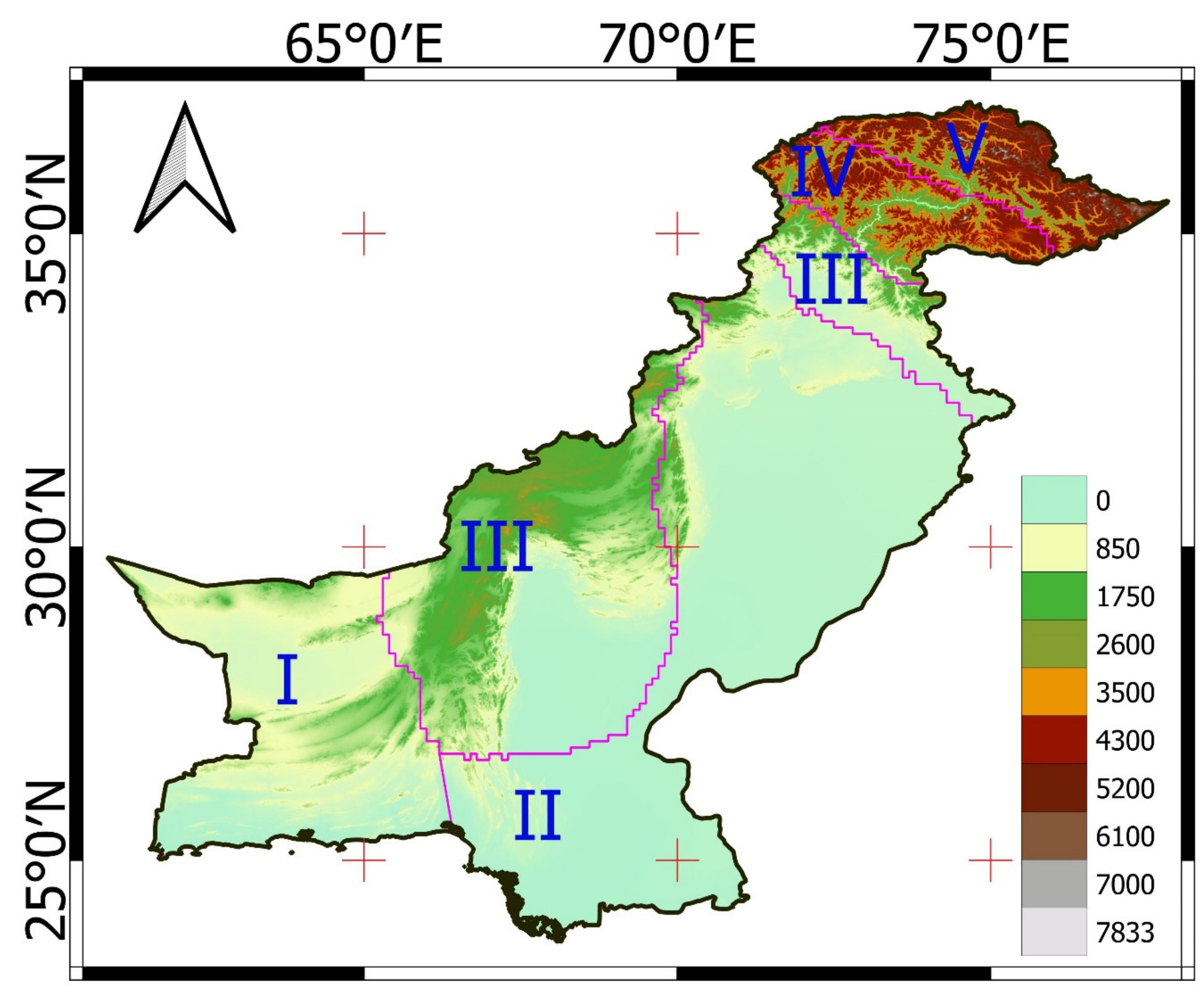
Pakistan is located in South Asia (SA) between latitudes 23–38° N and longitudes 61–78° E, with an area of 795,000 km2 spanning from mountains (more than 1000 m high) in the north to flat coasts in the south (Figure 1). It has a primarily dry climate, with a freezing winter (December to February) and a blistering summer (June to August) [49]. There are two seasons between winter and summer, a warm fall (September to November) and a dry spring (March to May) [50]. The temperatures in the country range from −15 °C in the northern Himalayas to more than 35 °C toward the southern coast. The precipitation ranges from less than 125 mm/year in the southwest to nearly 1000 mm/year in the north [51,52]. The country receives less than 500 mm of annual rainfall on most of its land area, with just a small section exceeding 1000 mm [53]. The yearly mean ET ranges from less than 10 mm/year in the north and more than 1900 mm/year in the south.
Pakistan has five climate zones based on temperature (Figure 1) [54]: the hot desert climate in the southwest (Zone I), the southeast and east plains with moderate winter and hot summer (Zone II), the elevated central region with cold winter and mild summer (Zone III), cold sub-Himalayan ranges in the north (Zone IV) and a cold mountain climate in the far north (Zone V).
2.2. Princeton Daily Data
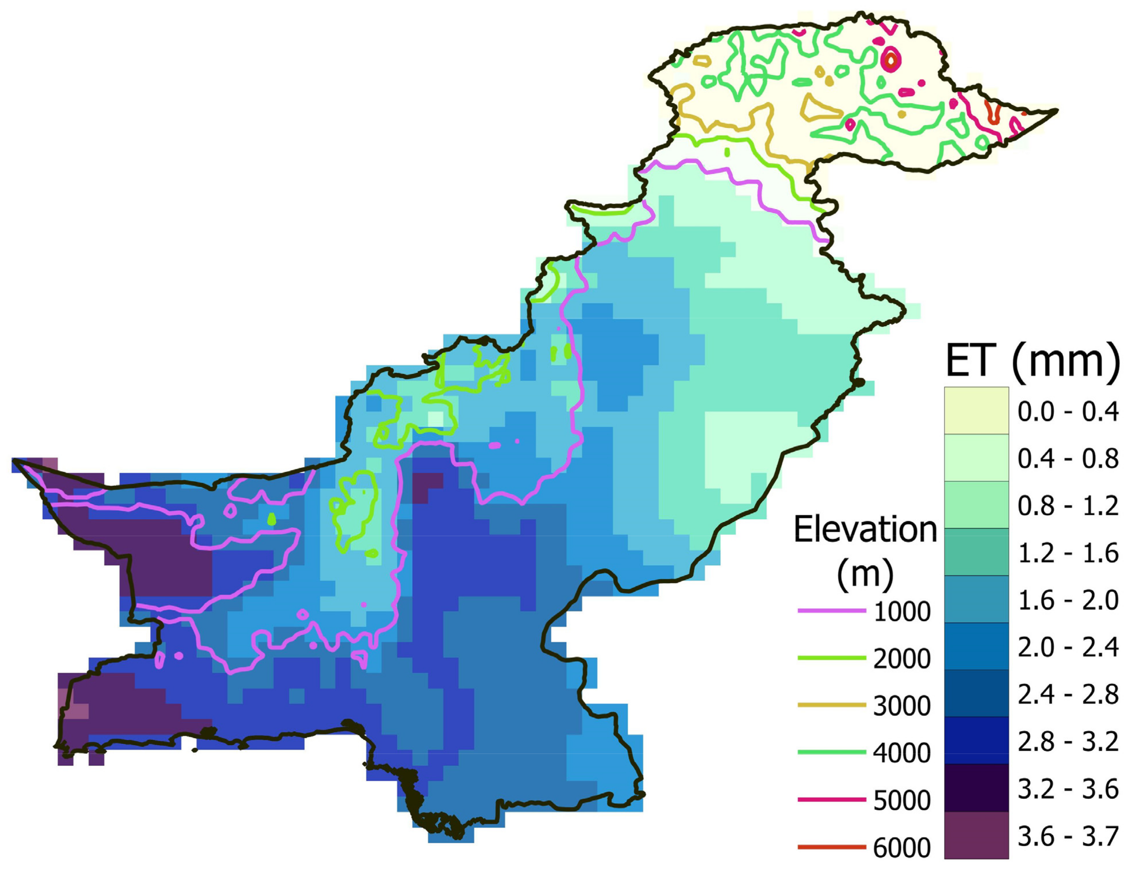
The study was accomplished using Princeton Global Meteorological Forcing (PGF) [55] daily maximum temperature (Tmax), minimum temperature (Tmin), relative humidity (RH), wind speed (WS), surface pressure (SP) and solar radiation (SR) data, as described in Table 1. The global in situ datasets are combined with the NCEP/NCAR reanalysis to generate the PGF data by the Land Surface Hydrology Research Group of Princeton University. Numerous studies used this data for global [56] and regional climate analysis, including in Africa [57,58,59,60,61], Asia [62,63,64], Canada [65] and the USA [66]. Several climatic studies have also been conducted in Pakistan using the PGF climate data [54,64,67,68]. Figure 2 presents the spatial distributions of daily average ET obtained using the Penman–Monteith (PM) method. It ranges from nearly 0.4 in the southern coastal zone to 3.7 mm in the western desert. ET decreases gradually to the north and reaches its minimum in the northern Himalayan region.
3. Method
3.1. Evapotranspiration (ET)
The pan ET data over a longer period at multiple locations are unavailable in Pakistan. Therefore, this study employed the PM [69] ET as the reference data. Studies across the globe showed a high correlation between monthly pan evaporation and the PM ET [31,35,36,38,70,71,72,73,74,75]. The ET is estimated using the PM equation as below [69]:
where es indicates vapor pressure, G is the soil heat flux, is the slope in vapor pressure versus temperature data, is the latent heat of evaporation and Tav is the mean temperature.
This study evaluated the performance of 30 empirical ET models (Table S1 in Supplementary Materials) to rank them for Pakistan according to required climate variables based on PM ET. The list of the empirical ET models, their class and the input needed are given in Table 2.
3.2. Performance Evaluation
The KGE was used to evaluate the performance of the 30 ET models at each PGF grid location. The KGE provides an integrated measurement of correlation, bias and variability [104]:
where is Pearson’s correlation, and and represent the mean and standard deviation of ET estimated using each empirical equation and PM ET, respectively. The KGE ranges from −∞ to an optimal value of 1.
The overall ranking of different ET models over Pakistan was also evaluated using different statistical metrics, including mean absolute error (MAE), root mean square error (RMSE), the coefficient of determination (R2), percent bias (PBIAS) and coefficient of agreement (md), as defined below:
where Oi is the PM ET, Si is the ET estimated using empirical equations, n represents the number of grids and and are the mean ET estimated using PM and empirical equations, respectively.
3.3. Multi-Criteria Group Decision Making (MCGDM)
The ET models were ranked for the whole of Pakistan using an MCGDM. In this approach, each model was provided with a weight based on the rank achieved by the model at different grid points (n) to calculate an integrated index (Ix). The weight of a model was set as an inverse of the rank. It means the best model was provided with a weight of 1 (1/1 = 1), the second-best model with a weight of 0.5 (1/2 = 0.5), the third-best model with a weight of 0.33 (1/3 = 0.33), and so on. The integrated index of a model is estimated as,
The models that obtained a rank of 10 or higher at a grid point were only considered for the final ranking. Otherwise, the model was considered incapable of estimating ET at the grid point and, thus, assigned a zero weight. The Ix value of different models was used to provide the final ranks of the models. A model with a higher Ix indicates its better performance in estimating ET for the whole of Pakistan [69].
4. Results
4.1. Ranking of ET Equations
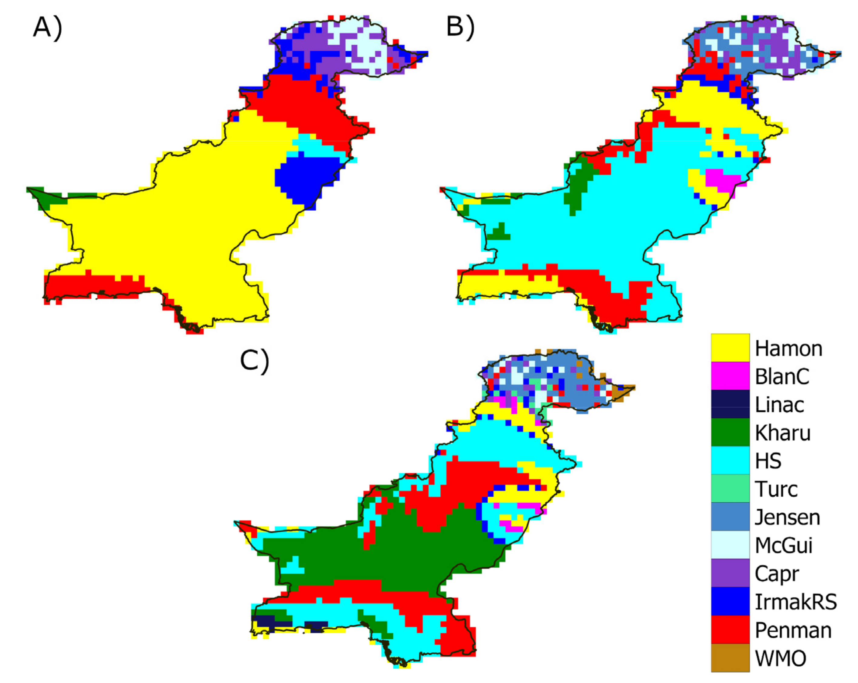
The ET was estimated using empirical equations at each grid over Pakistan. Estimated ET using different equations (Table 2) was compared with the PM ET using KGE. The ET models were ranked from 1 to 30 at each grid point based on KGE. Figure 3 shows the top three ET models at each grid point over Pakistan. More than 60% of the grids, mostly located in the middle and south, showed the temperature-based Hamon as the best model, while mass transfer-based Penman was the best in the southwest and upper-middle region. Radiation-based Irmak-RS, Caprio and McGuinness and temperature-based Hargreaves and Kharrufa were ranked first at a few grids in the north, east and southwest regions. Hargreaves was ranked as the second-best model at more than 50% of the girds, followed by Penman and Hamon. Kharrufa was ranked third in many grids in the south, followed by Penman and Hargreaves.
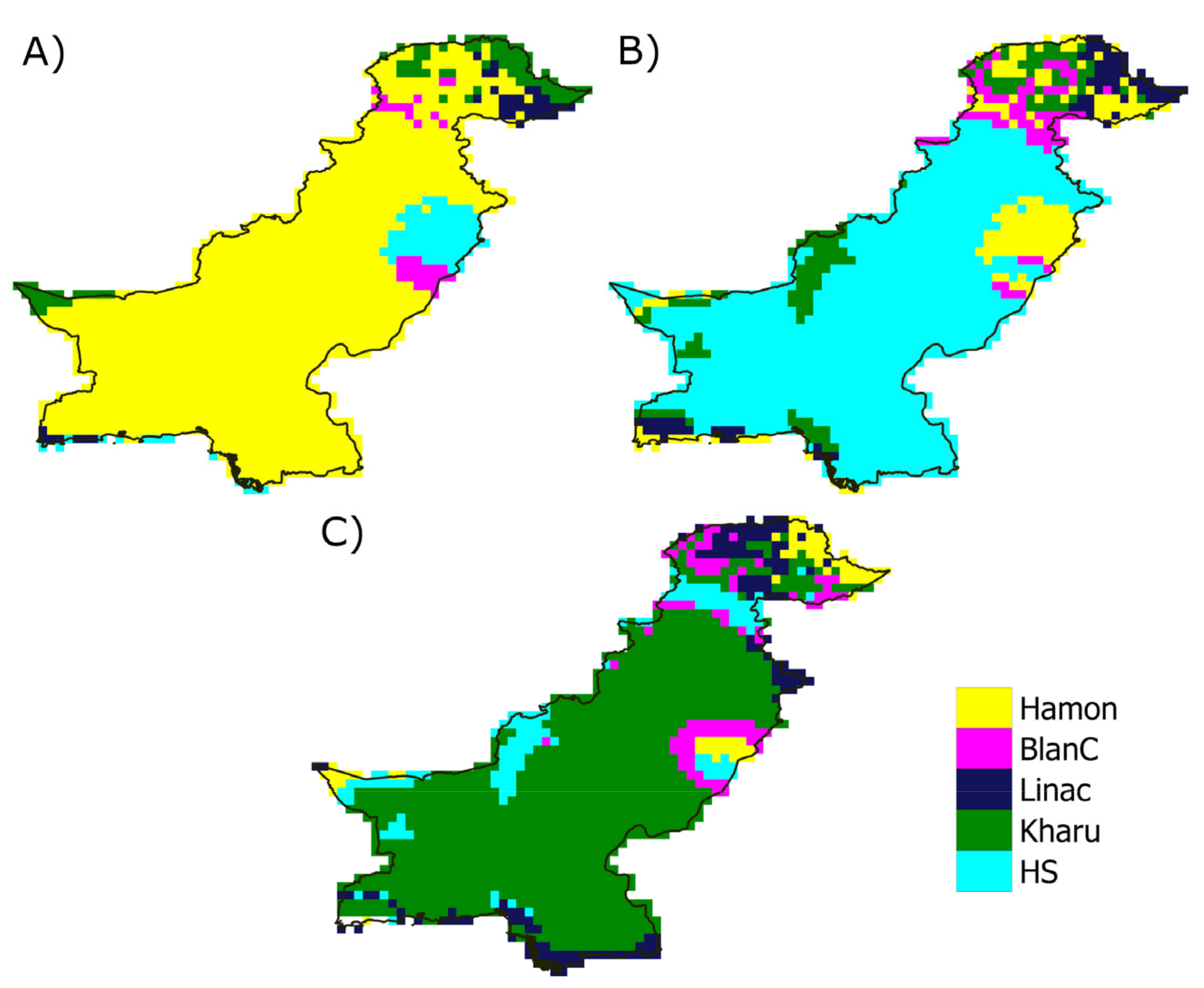
The present study also individually ranked temperature, radiation, mass transfer and combined ET models over Pakistan to reveal the best models in each category. Figure 4 shows the top three temperature-based ET models at each grid point over Pakistan. Hamon was ranked first in more than 80% of the grids. However, Hargreaves showed the best performance in the east and Kharrufa in the north and southeast regions. Hargreaves was ranked second in the middle and south, Hamon in the east, while the remaining four temperature-based equations showed better performance at different grids in the north. Kharrufa was ranked third in all regions, except in the east and north, where none of the temperature models showed dominating performance over the entire country.
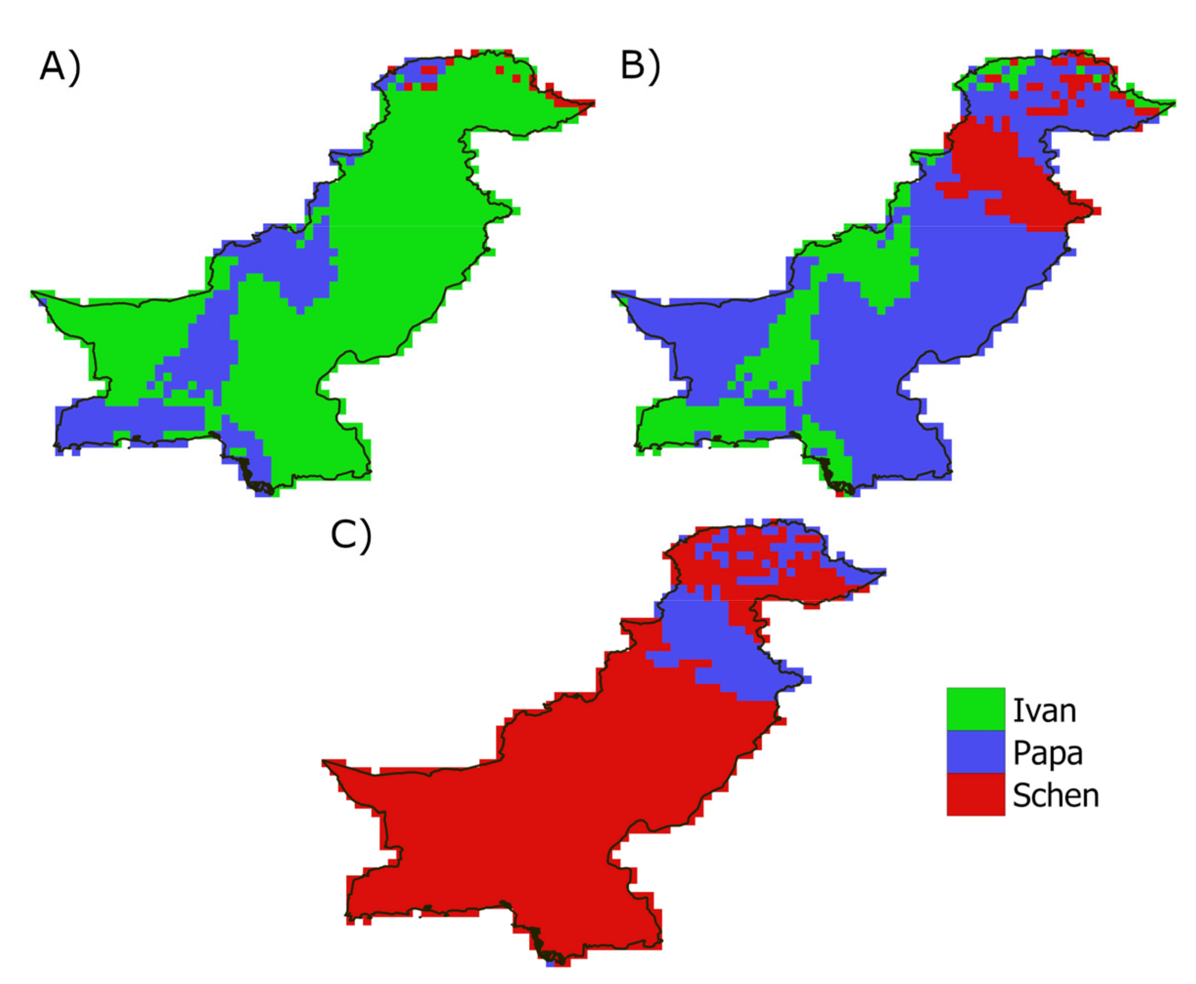
The performance of three relative humidity-based equations considered in this study is shown in Figure 5. The Ivanov model showed the best performance at more than 60% of the grids. The Papadakis model showed the best performance in the rest of the grids. However, Ivanov was ranked as the second-best at the grids, whereas Papadakis was ranked first. In the north, Schendel was ranked as the second-best model.
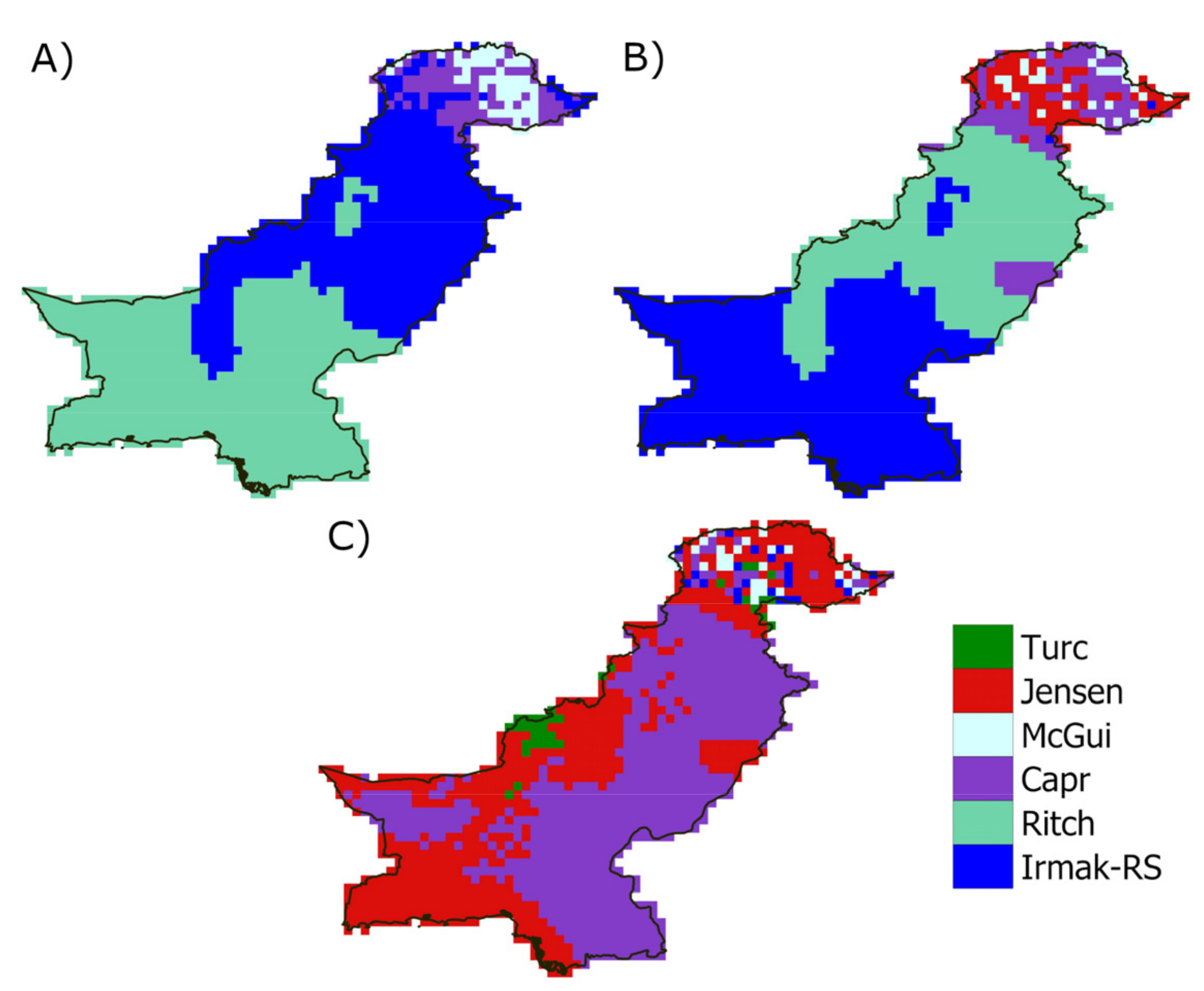
The performance of ten radiation-based models is shown in Figure 6. McGuinness–Bordne and Caprio were ranked first in the north, Irmak-RS was in the middle and Ritchie was in the south. Irmak-Rs was the second-best model in the south and Ritchie in the middle. Jensen–Haise was the third-best model in the north, east and south, while Caprio was in the middle and southeast.
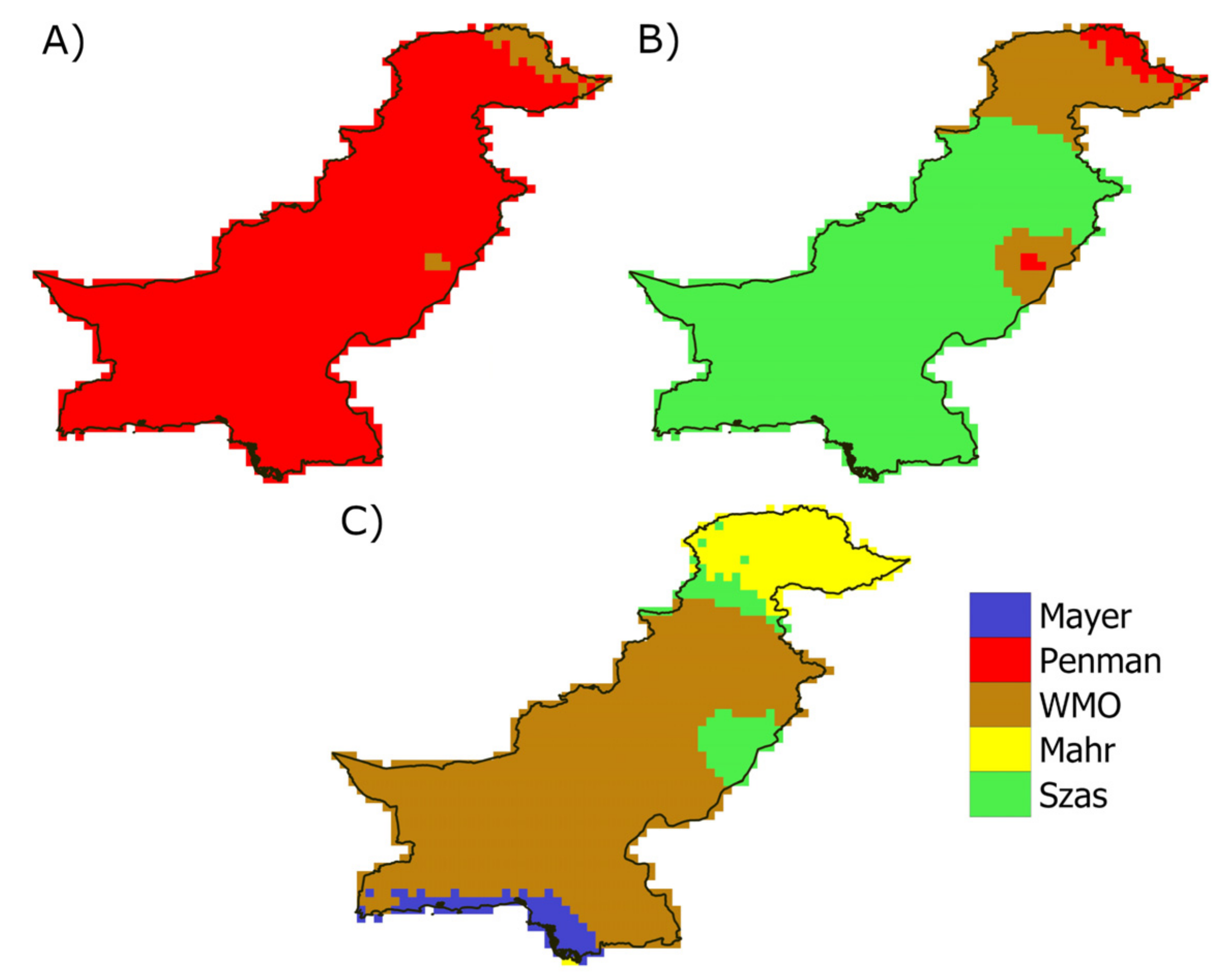
Among the mass transfer-based models, Penman was ranked first over the whole of Pakistan, except at some grids in the north, where WMO was the best (Figure 7). Szasz was ranked as the second-best model in the central and south, while Penman and WMO were in the north and east. WMO was ranked as the third-best model over most of Pakistan, except Mahringer in the north, Mayer along the southern coastline and Szasz in the east.
4.2. Ranking for the Whole of Pakistan
The top three ET models identified by MCGDM suitable for estimating ET for the whole of Pakistan are given in Table 3. The results showed that the Hamon model was ranked first among all ET models considered in this study, with an Ix of 1027.12. Penman ranked second (Ix = 599.71), followed by HS (Ix = 528.04). The results indicate a much higher performance of Hamon than other models in terms of Ix. Among the RH models, Ivan performed best (Ix = 147.03), followed by Papa (Ix = 99.06) and Schen (Ix = 21.12). In the case of radiation-based models, Irmak-RS performed best (Ix = 223.72), followed by Capr (Ix = 129.00) and McGui (Ix = 84.45). Among the mass transfer-based equations, Penman performed the best (Ix = 599.71), followed by Szas (Ix = 195.69) and WMO (Ix = 122.72). Overall, the temperature-based model’s ranking was much higher than other categories of models. Mass transfer-based models performed better than RH and radiation-based models. RH-based models showed the worst performance.
4.3. Validation of Ranking
The ranking of different models in different climate zones to replicate reference ET based on various statistical indices is presented in Table 4. The highest ranks (1 to 5) are presented using the bold values in the table. The intention was to show the capability of the best-ranked models in estimating reference ET in terms of different statistics. Different metrics ranked the ET models differently. However, Hamon was the best, followed by Penman, according to almost all indices for Zones I, II and III. Caprio was the best for Zones IV and V, followed by Irmak-RS. In contrast, Priestley–Taylor and Irmak-Rn showed the worst performance in all climate zones in terms of all indices.
4.4. Spatial Bias in Top-Ranked Models
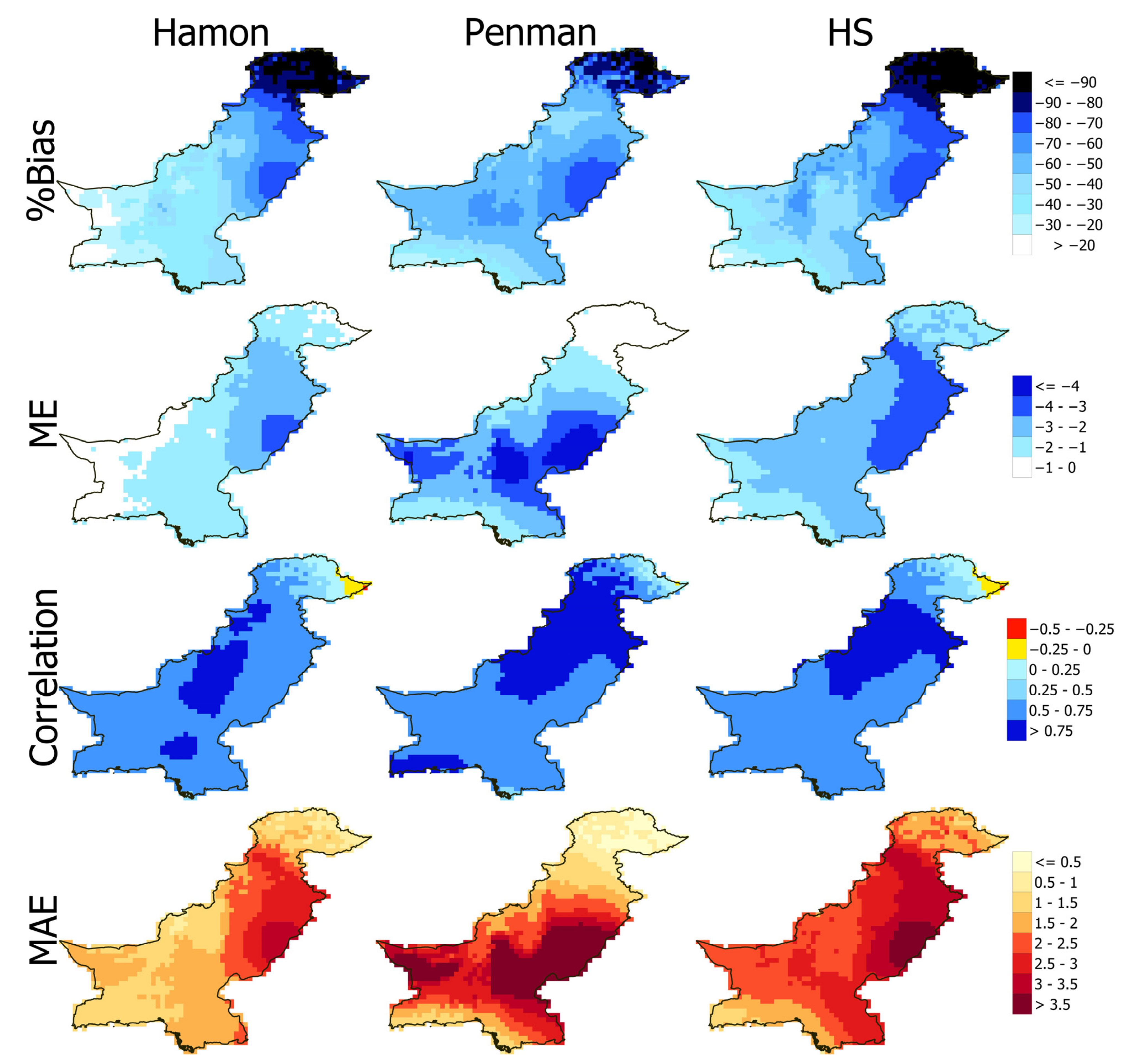
The spatial distribution of PBIAS, ME and correlation of the top-ranked models (Hamon, Penman and HS) is presented in Figure 8. The intention was to show the error in estimated ET by the models in different regions of Pakistan. The PBIAS of the models ranged from −15 to −100, indicating the underestimation of ET by the best models. The underestimation was more in the north cold region (up to −90%). Overall, Hamon showed the least PBIAS. It was near zero in the west and less than −50% in most of Pakistan. The mean error (ME) in Hamon ET was less than −4 mm at all grids over Pakistan. The error was nearly zero over a large area in the west. It was high (−3 to −4 mm) only over a small area in the central west. The results indicate that Hamon can estimate ET in most parts of Pakistan with a mean error of less than −3 mm. The correlation between ET estimated by the top three models and the PM model was above 0.5 at almost all grids over Pakistan, except in the far north. It should be noted that a correlation coefficient higher than 0.06 is statistically significant at p < 0.05 for 69 years of monthly data (828 months). The results indicate the selected models can estimate ET in Pakistan with less bias and high correlation.
5. Discussion
This study evaluated the suitability of various ET models in Pakistan. Numerous studies assessed the performance of different ET models in various regions of the world [40,46,74,105,106]. Different indices have been used for this purpose. The studies showed different models as the best in terms of different statistics [105]. The present study also showed different performances of ET models in terms of different statistical metrics (Table 4). This study used an integrated statistical metric, KGE, to assess the performance of ET models at each grid point to avoid contradictory results obtained using different statistical metrics. Decision making about the best models for the entire country based on different rankings of the models at different grid points is a difficult task. This study proposed an MCGDA approach to overcome this drawback. Therefore, it is expected that the rankings obtained in this study are reliable. This is also proved by the performance of the models in terms of a set of statistical metrics. Therefore, it can be remarked that Hamon is the best model for estimating ET in Pakistan after the PM method.
Assessment of the ET model’s performance revealed different models as the best in reproducing the PM ET in countries bordering Pakistan. For example, Nandagiri and Kovoor [40] compared seven commonly used ET equations and showed Hargreaves as the best at four stations in India. Trajkovic and Kolakovic [107] evaluated the performance of five ET models in the humid Balkan region and showed Turc to perform the best. Similarly, Peng et al. [108] showed Berti as the best model in mainland China. Niaghi et al. [105] showed Penman ET closest to PM ET in some locations of Iran. The ET models’ performance assessment studies are very limited in Pakistan. As reviewed in the Introduction section, the previous studies showed the analysis of only a few ET models at a few stations in the semiarid region of Pakistan. This is the first attempt to evaluate the ET model over Pakistan using robust methods. The study revealed the better performance of temperature-based models in Pakistan. It also established the temperature-based Hamon model as the best in estimating ET in Pakistan.
The findings of the study agree with other studies in nearby regions. Shirmohammadi-Aliakbarkhani and Saberali [109] evaluated the skill of several ET models at 13 locations in Iran, bordering Pakistan in the east. They also showed better performance of temperature-based models than others. Aparecido et al. [110] evaluated the performance of 19 ET models in Midwest Brazil and showed better performance of temperature-based models than others. Paparrizos et al. [111] also reported that temperature-based models are more reliable in estimating ET in different regions of Greece.
Several studies also reported Hamon is most reliable in estimating ET in different regions [112,113,114] and, thus, agree with the finding of this study. Federer et al. [114] evaluated different ET models globally and reported Hamon as the best for a wide range of climates. Vörösmarty et al. [113] also evaluated eleven ET methods for a diverse range of climates in the US and showed Haman as the most reliable. Shirmohammadi-Aliakbarkhani and Saberali [109] also ranked Hamon as one of the best models for estimating ET in Iran. Askar et al. [115] evaluated seven ET models in peninsular Malaysia and showed Hamon as the most sensitive model. Paparrizos et al. [111] showed different versions of Hamon as the best model for estimating ET in different climates of Greece. Singh et al. [43] showed the efficiency of Hamon in estimating ET from satellite data in agricultural regions of India. Ansorge and Beran [116] compared the performance of several temperature-based ET models with observed pan evaporation data and showed higher correlation and least error in Homon estimated ET. However, several studies also showed very poor performance of Hamon [117,118]. This indicates the need for performance evaluation of ET models before their use in an area.
Hamon provides the best estimation of ET in Pakistan, but it underestimates ET all over the country, except in the far west. McCabe et al. [119] also showed an underestimation of ET using the Hamon method over the United States, except in the country’s southwest. They proposed calibration of the Hamon model for the region of interest to enhance the model performance. This can be recommended for future work.
The spatial distribution of models’ ranking (Figure 3, Figure 4, Figure 5, Figure 6 and Figure 7) with respect to elevation (Figure 2) revealed a large heterogeneity in models’ performance in the elevated northern Pakistan. No ET model was found best over most grid points in the elevated regions. In contrast, a consistent performance of the models was noticed in the southern plains. This may be due to high variability of climate with elevation in the sub-Himalayan region. Therefore, the best-performing models (Hamon, Penman and HS) were selected for the whole of Pakistan using MCGDM, a large bias and low correlation with PM ET in the elevated regions.
The PGF meteorological data were used to estimate ET in this study, considering its reliability in climatic studies in Pakistan as reported in the literature [54,64,67,68]. It should be noted that the rankings of the ET models may change if different datasets, such as ERA5 or National Centers for Environmental Prediction (NCEP), are used. Khan et al. [67] employed three datasets developed by three organizations to assess the performance of global climate models in simulating historical temperatures over Pakistan. They showed significant variability of model performance for different datasets. Multiple datasets can be used in the future to assess the ranking sensitivity of ET models to the datasets.
6. Conclusions
This study assessed the performance of 30 empirical ET models for Pakistan, considering PM ET as the reference. The intention was to rank them according to their performance to allow users to select the most suitable model according to data availability. The PGF daily climate data for 1948–2016 was used for this purpose. The study revealed Hamon as the best model for most of Pakistan, followed by Hargreaves–Samani and Penman. Hamon uses only mean temperature for ET estimation. Therefore, it can be used for a reliable estimate of ET over most of Pakistan using only temperature. All global climate models simulate temperature for different climate change scenarios. Those simulated data could be used for reliable projection of ET of Pakistan using the Hamon model. However, it should be noted that Hamon estimated ET is prone to an average −50.2% bias which also varies spatially. Therefore, estimated ET using the Hamon model should be used for practice with caution. The estimated bias in the Hamon and other models presented in this study can be utilized for bias correction of ET before its application. This study considered 30 empirical daily ET estimation models. In the future, more ET models can be considered for performance evaluation, particularly monthly ET models such as Thornwaite, which are widely used for drought estimation.
Supplementary Materials
The following supporting information can be downloaded at: https://www.mdpi.com/article/10.3390/land11122168/s1, Table S1: List of the empirical ET equations and applications.
Author Contributions
Conceptualization, N.K. and S.S.; methodology, M.M.H. and N.K.; software, S.S.; validation, M.M.H. and S.S.; formal analysis, M.M.H. and N.K.; investigation, M.M.H. and N.K.; resources, M.M.H., M.K.I.M. and S.S.; data curation, M.M.H., M.K.I.M. and S.S.; writing—original draft preparation, M.M.H. and N.K.; writing—review and editing, M.K.I.M. and S.S.; visualization, M.M.H.; supervision, S.S.; project administration, S.S.; funding acquisition, S.S. All authors have read and agreed to the published version of the manuscript.
Funding
This research received financial support through UTM High Impact Grant No. 09G07.
Data Availability Statement
Not applicable.
Acknowledgments
We are grateful to Universiti Teknologi Malaysia (UTM) for providing financial support to complete this study through UTM High Impact Grant No. 09G07.
Conflicts of Interest
The authors declare no conflict of interest.
References
- Shahid, S. Impact of climate change on irrigation water demand of dry season Boro rice in northwest Bangladesh. Clim. Chang. 2011, 105, 433–453. [Google Scholar] [CrossRef]
- Newton, I.H.; Islam, G.M.T.; Islam, A.S.; Razzaque, S.; Bala, S.K. A conjugate application of MODIS/Terra data and empirical method to assess reference evapotranspiration for the southwest region of Bangladesh. Environ. Earth Sci. 2021, 80, 223. [Google Scholar] [CrossRef]
- Fisher, J.B.; Malhi, Y.; Bonal, D.; Da Rocha, H.R.; De Araújo, A.C.; Gamo, M.; Goulden, M.L.; Rano, T.H.; Huete, A.R.; Kondo, H.; et al. The land-atmosphere water flux in the tropics. Glob. Chang. Biol. 2009, 15, 2694–2714. [Google Scholar] [CrossRef]
- Wigmosta, M.S.; Vail, L.W.; Lettenmaier, D.P. A distributed hydrology-vegetation model for complex terrain. Water Resour. Res. 1994, 30, 1665–1679. [Google Scholar] [CrossRef]
- Jaber, H.S.; Mansor, S.; Pradhan, B.; Ahmad, N. Rainfall–runoff modelling and water balance analysis for Al-Hindiyah barrage, Iraq using remote sensing and GIS. Geocarto Int. 2017, 32, 1407–1420. [Google Scholar] [CrossRef]
- Salem, G.S.A.; Kazama, S.; Shahid, S.; Dey, N.C. Impact of temperature changes on groundwater levels and irrigation costs in a groundwater-dependent agricultural region in Northwest Bangladesh. Hydrol. Res. Lett. 2017, 11, 85–91. [Google Scholar] [CrossRef] [Green Version]
- Sadeghfam, S.; Hassanzadeh, Y.; Nadiri, A.A.; Khatibi, R. Mapping groundwater potential field using catastrophe fuzzy membership functions and Jenks optimization method: A case study of Maragheh-Bonab plain, Iran. Environ. Earth Sci. 2016, 75, 545. [Google Scholar] [CrossRef]
- Cambraia Neto, A.J.; Rodrigues, L.N. Evaluation of groundwater recharge estimation methods in a watershed in the Brazilian Savannah. Environ. Earth Sci. 2020, 79, 140. [Google Scholar] [CrossRef]
- Ismail, T.; Harun, S.; Zainudin, Z.M.; Shahid, S.; Fadzil, A.B.; Sheikh, U.U. Development of an optimal reservoir pumping operation for adaptation to climate change. KSCE J. Civ. Eng. 2017, 21, 467–476. [Google Scholar] [CrossRef]
- Mohsenipour, M.; Shahid, S.; Chung, E.-S.; Wang, X.-J. Changing Pattern of Droughts during Cropping Seasons of Bangladesh. Water Resour. Manag. 2018, 32, 1555–1568. [Google Scholar] [CrossRef]
- Shiru, M.S.; Shahid, S.; Alias, N.; Chung, E.S. Trend analysis of droughts during crop growing seasons of Nigeria. Sustainability 2018, 10, 871. [Google Scholar] [CrossRef] [Green Version]
- Salehie, O.; Hamed, M.M.; bin Ismail, T.; Shahid, S. Projection of droughts in Amu river basin for shared socioeconomic pathways CMIP6. Theor. Appl. Climatol. 2022, 149, 1009–1027. [Google Scholar] [CrossRef]
- Hamed, M.M.; Nashwan, M.S.; Shahid, S. Inter-comparison of Historical Simulation and Future Projection of Rainfall and Temperature by CMIP5 and CMIP6 GCMs Over Egypt. Int. J. Climatol. 2022, 42, 4316–4332. [Google Scholar] [CrossRef]
- Yang, J.; Xie, B.; Zhang, D.; Tao, W. Climate and land use change impacts on water yield ecosystem service in the Yellow River Basin, China. Environ. Earth Sci. 2021, 80, 72. [Google Scholar] [CrossRef]
- Wada, Y.; van Beek, L.P.H.; Bierkens, M.F.P. Modelling global water stress of the recent past: On the relative importance of trends in water demand and climate variability. Hydrol. Earth Syst. Sci. 2011, 15, 3785–3808. [Google Scholar] [CrossRef] [Green Version]
- Poonia, V.; Das, J.; Goyal, M.K. Impact of climate change on crop water and irrigation requirements over eastern Himalayan region. Stoch. Environ. Res. Risk Assess 2021, 35, 1175–1188. [Google Scholar] [CrossRef]
- Jiang, T.; Sun, S.; Li, Z.; Li, Q.; Lu, Y.; Li, C.; Wang, Y.; Wu, P. Vulnerability of crop water footprint in rain-fed and irrigation agricultural production system under future climate scenarios. Agric. For. Meteorol. 2022, 326, 109164. [Google Scholar] [CrossRef]
- Ahmed, K.; Shahid, S.; Nawaz, N. Impacts of climate variability and change on seasonal drought characteristics of Pakistan. Atmos. Res. 2018, 214, 364–374. [Google Scholar] [CrossRef]
- Hamed, M.M.; Nashwan, M.S.; Shahid, S. A novel selection method of CMIP6 GCMs for robust climate projection. Int. J. Climatol. 2022, 42, 4258–4272. [Google Scholar] [CrossRef]
- Rana, G.; Katerji, N. Measurement and estimation of actual evapotranspiration in the field under Mediterranean climate: A review. Eur. J. Agron. 2000, 13, 125–153. [Google Scholar] [CrossRef]
- Tao, H.; Diop, L.; Bodian, A.; Djaman, K.; Ndiaye, P.M.; Yaseen, Z.M. Reference evapotranspiration prediction using hybridized fuzzy model with firefly algorithm: Regional case study in Burkina Faso. Agric. Water Manag. 2018, 208, 140–151. [Google Scholar] [CrossRef]
- Zhang, K.; Kimball, J.S.; Running, S.W. A review of remote sensing based actual evapotranspiration estimation. Water 2016, 3, 834–853. [Google Scholar] [CrossRef]
- Liou, Y.A.; Kar, S.K. Evapotranspiration estimation with remote sensing and various surface energy balance algorithms-a review. Energies 2014, 7, 2821–2849. [Google Scholar] [CrossRef] [Green Version]
- Noumonvi, K.D.; Ferlan, M.; Eler, K.; Alberti, G.; Peressotti, A.; Cerasoli, S. Estimation of Carbon Fluxes from Eddy Covariance Data and Satellite-Derived Vegetation Indices in a Karst Grassland (Podgorski Kras, Slovenia). Remote Sens. 2019, 11, 649. [Google Scholar] [CrossRef] [Green Version]
- Ha, W.; Kolb, T.E.; Springer, A.E.; Dore, S.; O’Donnell, F.C.; Martinez Morales, R.; Masek Lopez, S.; Koch, G.W. Evapotranspiration comparisons between eddy covariance measurements and meteorological and remote-sensing-based models in disturbed ponderosa pine forests. Ecohydrology 2015, 8, 1335–1350. [Google Scholar] [CrossRef]
- Muhammad, M.K.I.; Shahid, S.; Ismail, T.; Harun, S.; Kisi, O.; Yaseen, Z.M. The development of evolutionary computing model for simulating reference evapotranspiration over Peninsular Malaysia. Theor. Appl. Climatol. 2021, 144, 1419–1434. [Google Scholar] [CrossRef]
- Pereira, A.R.; Nova, N.A.V.; Sediyama, G.C. Evapo (Transpi) Ração; FEALQ: Piracicaba, Brazil, 1997. [Google Scholar]
- Kumari, N.; Srivastava, A. An Approach for Estimation of Evapotranspiration by Standardizing Parsimonious Method. Agric. Res. 2020, 9, 301–309. [Google Scholar] [CrossRef]
- Douglas, E.M.; Jacobs, J.M.; Sumner, D.M.; Ray, R.L. A comparison of models for estimating potential evapotranspiration for Florida land cover types. J. Hydrol. 2009, 373, 366–376. [Google Scholar] [CrossRef]
- Ankur, S.; Bhabagrahi, S.; Singh, R.N.; Rajendra, S. Evaluation of Variable-Infiltration Capacity Model and MODIS-Terra Satellite-Derived Grid-Scale Evapotranspiration Estimates in a River Basin with Tropical Monsoon-Type Climatology. J. Irrig. Drain. Eng. 2017, 143, 4017028. [Google Scholar] [CrossRef] [Green Version]
- Muhammad, M.K.I.; Nashwan, M.S.; Shahid, S.; bin Ismail, T.; Song, Y.H.; Chung, E.S. Evaluation of empirical reference evapotranspiration models using compromise programming: A case study of Peninsular Malaysia. Sustainability 2019, 11, 4267. [Google Scholar] [CrossRef]
- Penman, H.L. Natural evaporation from open water, bare soil and grass. Proc. R. Soc. Lond. Ser. A Math. Phys. Sci. 1948, 193, 120–145. [Google Scholar]
- Nashwan, M.S.; Shahid, S.; Chung, E.-S.S. Development of high-resolution daily gridded temperature datasets for the central north region of Egypt. Sci. Data 2019, 6, 138. [Google Scholar] [CrossRef] [Green Version]
- Ahmed, K.; Shahid, S.; Ali, R.O.; Bin Harun, S.; Wang, X.J. Evaluation of the performance of gridded precipitation products over Balochistan province, Pakistan. Desalin. Water Treat. 2017, 79, 73–86. [Google Scholar] [CrossRef]
- Hosseinzadeh Talaee, P.; Tabari, H.; Abghari, H. Pan evaporation and reference evapotranspiration trend detection in western Iran with consideration of data persistence. Hydrol. Res. 2014, 45, 213–225. [Google Scholar] [CrossRef]
- Song, X.; Lu, F.; Xiao, W.; Zhu, K.; Zhou, Y.; Xie, Z. Performance of 12 reference evapotranspiration estimation methods compared with the Penman–Monteith method and the potential influences in northeast China. Meteorol. Appl. 2019, 26, 83–96. [Google Scholar] [CrossRef] [Green Version]
- Sobh, M.T.; Nashwan, M.S.; Amer, N. High Resolution Reference Evapotranspiration for Arid Egypt: Comparative analysis and evaluation of empirical and artificial intelligence models. Int. J. Climatol. 2022, 1–21. [Google Scholar] [CrossRef]
- Tabari, H.; Grismer, M.E.; Trajkovic, S. Comparative analysis of 31 reference evapotranspiration methods under humid conditions. Irrig. Sci. 2013, 31, 107–117. [Google Scholar] [CrossRef]
- Al-Mukhtar, M. Modeling the monthly pan evaporation rates using artificial intelligence methods: A case study in Iraq. Environ. Earth Sci. 2021, 80, 39. [Google Scholar] [CrossRef]
- Nandagiri, L.; Kovoor, G.M. Performance Evaluation of Reference Evapotranspiration Equations across a Range of Indian Climates. J. Irrig. Drain. Eng. 2006, 132, 238–249. [Google Scholar] [CrossRef]
- Wei, G.; Zhang, X.; Ye, M.; Yue, N.; Kan, F. Bayesian performance evaluation of evapotranspiration models based on eddy covariance systems in an arid region. Hydrol. Earth Syst. Sci. 2019, 23, 2877–2895. [Google Scholar] [CrossRef] [Green Version]
- Ndulue, E.; Onyekwelu, I.; Ogbu, K.N.; Ogwo, V. Performance evaluation of solar radiation equations for estimating reference evapotranspiration (ETo) in a humid tropical environment. J. Water Land Dev. 2019, 42, 124–135. [Google Scholar] [CrossRef]
- Singh, P.; Srivastava, P.K.; Mall, R.K. Estimation of potential evapotranspiration using INSAT-3D satellite data over an agriculture area. In Agricultural Water Management; Srivastava, P.K., Gupta, M., Tsakiris, G., Quinn, N.W., Eds.; Academic Press: Cambridge, MA, USA, 2021; pp. 143–155. ISBN 978-0-12-812362-1. [Google Scholar]
- Ahmed, K.; Shahid, S.; Bin Harun, S.; Wang, X. Characterization of seasonal droughts in Balochistan Province, Pakistan. Stoch. Environ. Res. Risk Assess. 2016, 30, 747–762. [Google Scholar] [CrossRef]
- Kyaw, A.K.; Hamed, M.M.; Shahid, S. Spatiotemporal Changes in Universal Thermal Climate Index Over South Asia. SSRN Electron. J. 2022, 1–32. [Google Scholar] [CrossRef]
- Azhar, A.H.; Masood, M.; Nabi, G.; Basharat, M. Performance Evaluation of Reference Evapotranspiration Equations Under Semiarid Pakistani Conditions. Arab. J. Sci. Eng. 2014, 39, 5509–5520. [Google Scholar] [CrossRef]
- Habeeb, R.; Zhang, X.; Hussain, I.; Hashmi, M.Z.; Elashkar, E.E.; Khader, J.A.; Soudagar, S.S.; Shoukry, A.M.; Ali, Z.; Al-Deek, F.F. Statistical analysis of modified Hargreaves equation for precise estimation of reference evapotranspiration. Tellus A Dyn. Meteorol. Oceanogr. 2021, 73, 1–12. [Google Scholar] [CrossRef]
- Nashwan, M.S.; Shahid, S. Symmetrical uncertainty and random forest for the evaluation of gridded precipitation and temperature data. Atmos. Res. 2019, 230, 104631. [Google Scholar] [CrossRef]
- Khan, N.; Shahid, S.; Sharafati, A.; Yaseen, Z.M.; Ismail, T.; Ahmed, K.; Nawaz, N. Determination of cotton and wheat yield using the standard precipitation evaporation index in Pakistan. Arab. J. Geosci. 2021, 14, 2035. [Google Scholar] [CrossRef]
- Sheikh, M.M. Drought management and prevention in Pakistan. In Proceedings of the COMSATS 1st Meeting on Water Resources in the South: Present Scenario and Future Prospects, Islamabad, Pakistan, 1–2 November 2001; Volume 1. [Google Scholar]
- Yasmeen, F.; Hameed, S. Forecasting of Rainfall in Pakistan via Sliced Functional Times Series (SFTS). World Environ. 2018, 8, 1–14. [Google Scholar] [CrossRef]
- Iqbal, Z.; Shahid, S.; Ahmed, K.; Ismail, T.; Nawaz, N. Spatial distribution of the trends in precipitation and precipitation extremes in the sub-Himalayan region of Pakistan. Theor. Appl. Climatol. 2019, 137, 2755–2769. [Google Scholar] [CrossRef]
- Ahmed, K.; Shahid, S.; Chung, E.-S.; Ismail, T.; Wang, X.-J. Spatial distribution of secular trends in annual and seasonal precipitation over Pakistan. Clim. Res. 2017, 74, 95–107. [Google Scholar] [CrossRef]
- Khan, N.; Shahid, S.; Ismail, T.; Ahmed, K.; Nawaz, N. Trends in heat wave related indices in Pakistan. Stoch. Environ. Res. Risk Assess. 2019, 33, 287–302. [Google Scholar] [CrossRef]
- Sheffield, J.; Goteti, G.; Wood, E.F. Development of a 50-year high-resolution global dataset of meteorological forcings for land surface modeling. J. Clim. 2006, 19, 3088–3111. [Google Scholar] [CrossRef] [Green Version]
- Tian, W.; Liu, X.; Wang, K.; Bai, P.; Liu, C.; Liang, X. Estimation of global reservoir evaporation losses. J. Hydrol. 2022, 607, 127524. [Google Scholar] [CrossRef]
- Nashwan, M.S.; Shahid, S. Spatial distribution of unidirectional trends in climate and weather extremes in Nile river basin. Theor. Appl. Climatol. 2019, 137, 1181–1199. [Google Scholar] [CrossRef]
- Nashwan, M.S.; Shahid, S.; Abd Rahim, N. Unidirectional trends in annual and seasonal climate and extremes in Egypt. Theor. Appl. Climatol. 2019, 136, 457–473. [Google Scholar] [CrossRef]
- Onyutha, C.; Acayo, G.; Nyende, J. Analyses of Precipitation and Evapotranspiration Changes across the Lake Kyoga Basin in East Africa. Water 2020, 12, 1134. [Google Scholar] [CrossRef]
- Mubialiwo, A.; Onyutha, C.; Abebe, A. Historical Rainfall and Evapotranspiration Changes over Mpologoma Catchment in Uganda. Adv. Meteorol. 2020, 2020, 8870935. [Google Scholar] [CrossRef]
- Mubialiwo, A.; Chelangat, C.; Onyutha, C. Changes in precipitation and evapotranspiration over Lokok and Lokere catchments in Uganda. Bull. Atmos. Sci. Technol. 2021, 2, 2. [Google Scholar] [CrossRef]
- Pour, S.H.; Wahab, A.K.A.; Shahid, S.; Wang, X. Spatial pattern of the unidirectional trends in thermal bioclimatic indicators in Iran. Sustainability 2019, 11, 2287. [Google Scholar] [CrossRef] [Green Version]
- Houmsi, M.R.; Shiru, M.S.; Nashwan, M.S.; Ahmed, K.; Ziarh, G.F.; Shahid, S.; Chung, E.S.; Kim, S. Spatial shift of aridity and its impact on land use of Syria. Sustainability 2019, 11, 7047. [Google Scholar] [CrossRef] [Green Version]
- Khan, N.; Shahid, S.; Ahmed, K.; Wang, X.; Ali, R.; Ismail, T.; Nawaz, N. Selection of GCMs for the projection of spatial distribution of heat waves in Pakistan. Atmos. Res. 2020, 233, 104688. [Google Scholar] [CrossRef]
- Wong, J.S.; Yassin, F.; Famiglietti, J.S.; Pomeroy, J.W. A streamflow-oriented ranking-based methodological framework to combine multiple precipitation datasets across large river basins. J. Hydrol. 2021, 603, 127174. [Google Scholar] [CrossRef]
- Tran, H.; Zhang, J.; O’Neill, M.M.; Ryken, A.; Condon, L.E.; Maxwell, R.M. A hydrological simulation dataset of the Upper Colorado River Basin from 1983 to 2019. Sci. Data 2022, 9, 16. [Google Scholar] [CrossRef] [PubMed]
- Khan, N.; Shahid, S.; Ahmed, K. Performance assessment of general circulation model in simulating daily precipitation and temperature using multiple gridded datasets. Water 2018, 10, 1793. [Google Scholar] [CrossRef] [Green Version]
- Khan, N.; Shahid, S.; Juneng, L.; Ahmed, K.; Ismail, T.; Nawaz, N. Prediction of heat waves in Pakistan using quantile regression forests. Atmos. Res. 2019, 221, 1–11. [Google Scholar] [CrossRef]
- Allen, R.G.; Pereira, L.S.; Raes, D.; Smith, M. Crop Evapotranspiration—Guidelines for Computing Crop Water Requirements; FAO Irrigation and Drainage Paper 56; FAO: Rome, Italy, 1998; Volume 300, p. D05109. [Google Scholar]
- Bogawski, P.; Bednorz, E. Comparison and Validation of Selected Evapotranspiration Models for Conditions in Poland (Central Europe). Water Resour. Manag. 2014, 28, 5021–5038. [Google Scholar] [CrossRef] [Green Version]
- Hazrat Ali, M.; Teang Shui, L.; Chee Yan, K.; Eloubaidy, A.F.; Chee Van, K. Modelling Evaporation and Evapotranspiration under Temperature Change in Malaysia. Pertanika J. Sci. Technol. 2000, 8, 191–204. [Google Scholar]
- Ali, M.H.; Shui, L.T. Potential evapotranspiration model for muda irrigation project, Malaysia. Water Resour. Manag. 2009, 23, 57–69. [Google Scholar] [CrossRef]
- Tukimat, N.N.A.; Harun, S.; Shahid, S. Comparison of different methods in estimating potential évapotranspiration at Muda Irrigation Scheme of Malaysia. J. Agric. Rural Dev. Trop. Subtrop. 2012, 113, 77–85. [Google Scholar]
- Djaman, K.; Balde, A.B.; Sow, A.; Muller, B.; Irmak, S.; N’Diaye, M.K.; Manneh, B.; Moukoumbi, Y.D.; Futakuchi, K.; Saito, K. Evaluation of sixteen reference evapotranspiration methods under sahelian conditions in the Senegal River Valley. J. Hydrol. Reg. Stud. 2015, 3, 139–159. [Google Scholar] [CrossRef] [Green Version]
- Gocic, M.; Trajkovic, S. Analysis of trends in reference evapotranspiration data in a humid climate. Hydrol. Sci. J. 2014, 59, 165–180. [Google Scholar] [CrossRef]
- Hamon, W.R. Computation of direct runoff amounts from storm rainfall. Int. Assoc. Sci. Hydrol. Publ. 1963, 63, 52–62. [Google Scholar]
- Doorenbos, J.; Pruitt, W.O. Crop Water Requirements; FAO Irrigation and Drainage Paper 24; Land and Water Development Division, FAO: Rome, Italy, 1977; Volume 144. [Google Scholar]
- Linacre, E.T. A simple formula for estimating evaporation rates in various climates, using temperature data alone. Agric. Meteorol. 1977, 18, 409–424. [Google Scholar] [CrossRef]
- Kharrufa, N.S. Simplified equation for evapotranspiration in arid regions. Beitr. Hydrol. 1985, 5, 39–47. [Google Scholar]
- Hargreaves, G.; Samani, Z. Reference Crop Evapotranspiration from Temperature. Appl. Eng. Agric. 1985, 1, 96–99. [Google Scholar] [CrossRef]
- Trajkovic, S. Hargreaves versus Penman-Monteith under Humid Conditions. J. Irrig. Drain. Eng. 2007, 133, 38–42. [Google Scholar] [CrossRef]
- Ravazzani, G.; Corbari, C.; Morella, S.; Gianoli, P.; Mancini, M. Modified Hargreaves-Samani Equation for the Assessment of Reference Evapotranspiration in Alpine River Basins. J. Irrig. Drain. Eng. 2012, 138, 592–599. [Google Scholar] [CrossRef]
- Romanenko, V.A. Computation of the autumn soil moisture using a universal relationship for a large area. Proc. Ukr. Hydrometeorol. Res. Inst. 1961, 3, 12–25. [Google Scholar]
- Papadakis, J. Crop Ecologic Survey in Relation to Agricultural Development of Western Pakistan; Draft Report; FAO: Rome, Italy, 1965. [Google Scholar]
- Schendel, U. Vegetationswasserverbrauch und-wasserbedarf. Habilit. Kiel 1967, 137, 1–11. [Google Scholar]
- Makkink, G.F. Testing the Penman formula by means of lysimeters. J. Inst. Water Eng. 1957, 11, 277–288. [Google Scholar]
- Turc, L. Water requirements assessment of irrigation, potential evapotranspiration: Simplified and updated climatic formula. In Annales Agronomiques; L’Institut National de la Recherche Agronomique (INRA): Paris, France, 1961; Volume 12, pp. 13–49. [Google Scholar]
- Jensen, M.E.; Haise, H.R. Estimating evapotranspiration from solar radiation. J. Irrig. Drain. Div. 1963, 89, 15–41. [Google Scholar] [CrossRef]
- Priestley, C.H.B.; Taylor, R.J. On the assessment of surface heat flux and evaporation using large-scale parameters. Mon. Weather Rev. 1972, 100, 81–92. [Google Scholar] [CrossRef]
- McGuinness, J.L.; Bordne, E.F. A Comparison of Lysimeter-Derived Potential Evapotranspiration with Computed Values; U.S. Department of Agriculture: Washington, DC, USA, 1972; ISBN 0082-9811. [Google Scholar]
- Caprio, J. The solar thermal unit concept in problems related to plant development and potential evapotranspiration. In Phenology and Seasonality Modeling; Springer: Berlin/Heidelberg, Germany, 1974; pp. 353–364. [Google Scholar]
- Jones, J.W.; Ritchie, J.T. Crop Growth Models. Manag. Farm Irrig. Syst. 1990, 41, 63–69. [Google Scholar]
- Abtew, W. Evapotranspiration measurements and modeling for three wetland systems in south Florida. Water Resour. Bull. 1996, 32, 465–473. [Google Scholar] [CrossRef]
- Irmak, S.; Allen, R.G.; Whitty, E.B. Daily Grass and Alfalfa-Reference Evapotranspiration Estimates and Alfalfa-to-Grass Evapotranspiration Ratios in Florida. J. Irrig. Drain. Eng. 2003, 129, 360–370. [Google Scholar] [CrossRef]
- Dalton, J. On the constitution of mixed gases, on the force of steam of vapour from water and other liquids in different temperatures, both in a Torricellia vacuum and in air; on evaporation; and on the expansion of gases by heat. Mem. Lit. Philos. Soc. Manch. 1802, 5, 536–602. [Google Scholar]
- Trabert, W. Neue beobachtungen über verdampfungsgeschwindigkeiten. Meteorol. Z. 1896, 13, 261–263. [Google Scholar]
- Meyer, A. Über einige Zusammenhänge zwischen Klima und Boden in Europa. Ph.D. Thesis, ETH Zurich, Zurich, Switzerland, 1926. Volume 2. pp. 209–347. [Google Scholar]
- Rohwer, C. Evaporation from Free Water Surfaces; U.S. Department of Agriculture: Washington, DC, USA, 1931. [Google Scholar]
- Albrecht, F. Die Methoden zur Bestimmung der Verdunstung der natürlichen Erdoberfläche. Arch. Meteorol. Geophys. Bioklimatol. Ser. B 1950, 2, 1–38. [Google Scholar] [CrossRef]
- Brockamp, B.; Wenner, H. Verdunstungsmessungen auf den Steiner see bei münster. Dt. Gewässerkundl. Mitt. 1963, 7, 149–154. [Google Scholar]
- Gangopadhyaya, M. Measurement and Estimation of Evaporation and Evapotranspiration; Springer Science & Business Media: Geneva, Switzerland, 1966; Volume 83. [Google Scholar]
- Mahringer, W. Verdunstungsstudien am Neusiedler See. Arch. Meteorol. Geophys. Bioklimatol. Ser. B 1970, 18, 1–20. [Google Scholar] [CrossRef]
- Szász, G. A potenciális párolgás meghatározásának új módszere. Hidrol. Közlöny 1973, 10, 435–442. [Google Scholar]
- Gupta, H.V.; Kling, H.; Yilmaz, K.K.; Martinez, G.F. Decomposition of the mean squared error and NSE performance criteria: Implications for improving hydrological modelling. J. Hydrol. 2009, 377, 80–91. [Google Scholar] [CrossRef] [Green Version]
- Niaghi, A.R.; Majnooni-Heris, A.; Haghi, D.Z.; Mahtabi, G. Evaluate several potential evapotranspiration methods for regional use in Tabriz, Iran. J. Appl. Environ. Biol. Sci. 2013, 3, 31–41. [Google Scholar]
- Hu, Z.; Chen, X.; Chen, D.; Li, J.; Wang, S.; Zhou, Q.; Yin, G.; Guo, M. “Dry gets drier, wet gets wetter”: A case study over the arid regions of central Asia. Int. J. Climatol. 2019, 39, 1072–1091. [Google Scholar] [CrossRef]
- Trajkovic, S.; Kolakovic, S. Evaluation of reference evapotranspiration equations under humid conditions. Water Resour. Manag. 2009, 23, 3057–3067. [Google Scholar] [CrossRef]
- Peng, L.; Li, Y.; Feng, H. The best alternative for estimating reference crop evapotranspiration in different sub-regions of mainland China. Sci. Rep. 2017, 7, 5458. [Google Scholar] [CrossRef] [Green Version]
- Shirmohammadi-Aliakbarkhani, Z.; Saberali, S.F. Evaluating of eight evapotranspiration estimation methods in arid regions of Iran. Agric. Water Manag. 2020, 239, 106243. [Google Scholar] [CrossRef]
- Aparecido, L.E.d.O.; de Meneses, K.C.; Torsoni, G.B.; de Moraes, J.R.d.S.C.; Mesquita, D.Z. Accuracy of potential evapotranspiration models in different time scales. Rev. Bras. Meteorol. 2020, 35, 63–80. [Google Scholar] [CrossRef]
- Paparrizos, S.; Maris, F.; Matzarakis, A. Sensitivity analysis and comparison of various potential evapotranspiration formulae for selected Greek areas with different climate conditions. Theor. Appl. Climatol. 2017, 128, 745–759. [Google Scholar] [CrossRef]
- Lu, J.; Sun, G.; McNulty, S.G.; Amatya, D.M. A comparison of six potential evapotranspiration methods for regional use in the southeastern United States. J. Am. Water Resour. Assoc. 2005, 41, 621–633. [Google Scholar] [CrossRef]
- Vörösmarty, C.J.; Federer, C.A.; Schloss, A.L. Potential evaporation functions compared on US watersheds: Possible implications for global-scale water balance and terrestrial ecosystem modeling. J. Hydrol. 1998, 207, 147–169. [Google Scholar] [CrossRef]
- Federer, C.A.; Vörösmarty, C.; Fekete, B. Intercomparison of Methods for Calculating Potential Evaporation in Regional and Global Water Balance Models. Water Resour. Res. 1996, 32, 2315–2321. [Google Scholar] [CrossRef]
- Askari, M.; Mustafa, M.A.; Setiawan, B.I.; Soom, M.A.M.; Harun, S.; Abidin, M.R.Z.; Yusop, Z. A combined sensitivity analysis of seven potential evapotranspiration models. J. Teknol. 2015, 76, 61–68. [Google Scholar] [CrossRef] [Green Version]
- Ansorge, L.; Beran, A. Performance of simple temperature-based evaporation methods compared with a time series of pan evaporation measures from a standard 20 m2 tank. J. Water Land Dev. 2019, 41, 1–11. [Google Scholar] [CrossRef]
- Santos, R.D.S.; de Souza, M.H.C.; de Carvalho Bispo, R.; Ventura, K.M.; Bassoi, L.H. Comparação entre métodos de estimativa da evapotranspiração de referência para o município de Petrolina, PE. Irriga 2017, 1, 31–39. [Google Scholar] [CrossRef] [Green Version]
- Zhao, L.; Xu, F.; Xia, J.; Wu, H. Applicability of 12 PET estimation methods in different climate regions in China. Hydrol. Res. 2021, 52, 636–657. [Google Scholar] [CrossRef]
- McCabe, G.J.; Hay, L.E.; Bock, A.; Markstrom, S.L.; Atkinson, R.D. Inter-annual and spatial variability of Hamon potential evapotranspiration model coefficients. J. Hydrol. 2015, 521, 389–394. [Google Scholar] [CrossRef]
Figure 1.
Study area location with its topography along with the five main climate zones (I to V).

Figure 2.
Spatial variability of daily mean evapotranspiration (ET), estimated using Penman–Monteith (PM) method for the period 1948–2016 and the elevation.
Figure 2.
Spatial variability of daily mean evapotranspiration (ET), estimated using Penman–Monteith (PM) method for the period 1948–2016 and the elevation.

Figure 3.
Spatial distribution of ET models ranked (A) first, (B) second and (C) third at different grid points over Pakistan.
Figure 3.
Spatial distribution of ET models ranked (A) first, (B) second and (C) third at different grid points over Pakistan.

Figure 4.
Same as Figure 3, but for temperature-based models.
Figure 4.
Same as Figure 3, but for temperature-based models.

Figure 5.
Same as Figure 3, but for relative humidity-based models.
Figure 5.
Same as Figure 3, but for relative humidity-based models.

Figure 6.
Same as Figure 3, but for radiation-based models.
Figure 6.
Same as Figure 3, but for radiation-based models.

Figure 7.
Same as Figure 3, but for mass transfer-based models.
Figure 7.
Same as Figure 3, but for mass transfer-based models.

Figure 8.
Spatial distribution of MAE, ME, correlation coefficient and MAE of the top three ET models.
Figure 8.
Spatial distribution of MAE, ME, correlation coefficient and MAE of the top three ET models.


Table 1.
List of the data used in the present study.
| Dataset Name | Variables | Spatial Resolution | Temporal Extent | Source |
|---|---|---|---|---|
| Princeton Global Meteorological Forcing (PGF) | Tmax, Tmin, RH, WS, SP and SR | 0.25° × 0.25° | 1948–2016 | http://hydrology.princeton.edu/data/pgf/v3/0.25deg/daily/ (accessed on 1 May 2022) |
Table 2.
List of the empirical ET models used in this study, their class and input requirements.
| No | Model | References | Parameter | |
|---|---|---|---|---|
| Temperature-based | 1 | Hamon | [76] | T |
| 2 | Blaney–Criddle | [77] | T | |
| 3 | Linacre | [78] | T | |
| 4 | Kharufa | [79] | T | |
| 5 | Hargreaves–Samani | [80] | T, Tmin, Tmax, Ra | |
| 6 | Trajkovic | [81] | T, Tmin, Tmax, Ra | |
| 7 | Ravazzani | [82] | T, Tmin, Tmax, Ra | |
| RH-based | 1 | Ivanov | [83] | T, RH |
| 2 | Papadakis | [84] | T, RH | |
| 3 | Schendel | [85] | T, RH | |
| Radiation-based | 1 | Makkink | [86] | T, Rs |
| 2 | Turc | [87] | T, Rs, RH | |
| 3 | Jensen–Haise | [88] | T, Rs | |
| 4 | Priestley–Taylor | [89] | T, Rs, RH | |
| 5 | McGuinness–Bordne | [90] | T, Rs | |
| 6 | Caprio | [91] | T, Rs | |
| 7 | Ritchie | [92] | Tmin, Tmax, Rs | |
| 8 | Abtew | [93] | T, Rs | |
| 9 | Irmak-Rs | [94] | T, Rs | |
| 10 | Irmak-Rn | [94] | T, Rs, RH | |
| Mass transfer-based | 1 | Dalton | [95] | T, RH, u |
| 2 | Trabert | [96] | ||
| 3 | Meyer | [97] | ||
| 4 | Rohwer | [98] | ||
| 5 | Penman | [32] | ||
| 6 | Albrecht | [99] | ||
| 7 | Brockamp–Wenner | [100] | ||
| 8 | WMO | [101] | ||
| 9 | Mahringer | [102] | ||
| 10 | Szasz | [103] |
(Note: Tmin: minimum temperature (°C), T: mean temperature (°C), Tmax: maximum temperature (°C), Ra: extraterrestrial radiation (MJ/m2/day), Rs: solar radiation (MJ/m2/day), es is the saturation vapor pressure (hPa), RH: relative humidity (%), u: wind speed at 2 m (m/s)).
Table 3.
Ranking of different categories of ET model for the whole of Pakistan using multi-criteria group decision-making method.
Table 3.
Ranking of different categories of ET model for the whole of Pakistan using multi-criteria group decision-making method.
| 1st | 2nd | 3rd | |
|---|---|---|---|
| All equations rank | |||
| Model name | Hamon | Penman | HS |
| MCGDM Index | 1027.12 | 599.71 | 528.04 |
| Temperature-based equations rank | |||
| Model name | Hamon | HS | Kharu |
| MCGDM Index | 1027.12 | 528.04 | 349.59 |
| RH-based equations rank | |||
| Model name | Ivan | Papa | Schen |
| MCGDM Index | 147.03 | 99.06 | 21.12 |
| Radiation-based equations rank | |||
| Model name | Irmak-RS | Capr | McGui |
| MCGDM Index | 223.72 | 129.00 | 84.45 |
| Mass transfer-based equations rank | |||
| Model name | Penman | Szas | WMO |
| MCGDM Index | 599.71 | 195.69 | 112.72 |
Table 4.
Ranking of ET model in different climate zones based on different statistical indices. Bold values are 5 top raked models.
Table 4.
Ranking of ET model in different climate zones based on different statistical indices. Bold values are 5 top raked models.
| Model | KGE | md | PBIAS | NRMSE | ||||||||||||||||
|---|---|---|---|---|---|---|---|---|---|---|---|---|---|---|---|---|---|---|---|---|
| 1 | 2 | 3 | 4 | 5 | 1 | 2 | 3 | 4 | 5 | 1 | 2 | 3 | 4 | 5 | 1 | 2 | 3 | 4 | 5 | |
| hs | 3 | 2 | 2 | 23 | 24 | 3 | 11 | 7 | 22 | 11 | 3 | 5 | 5 | 22 | 23 | 4 | 11 | 7 | 21 | 16 |
| Makkink | 27 | 27 | 27 | 7 | 7 | 28 | 28 | 27 | 16 | 15 | 28 | 28 | 28 | 4 | 5 | 27 | 28 | 27 | 22 | 24 |
| Turc | 25 | 25 | 25 | 24 | 27 | 25 | 23 | 24 | 4 | 1 | 23 | 13 | 19 | 12 | 22 | 25 | 25 | 25 | 4 | 1 |
| PriesT | 30 | 30 | 30 | 30 | 30 | 30 | 30 | 30 | 30 | 30 | 30 | 30 | 30 | 30 | 30 | 30 | 30 | 30 | 30 | 30 |
| Dalt | 15 | 17 | 15 | 15 | 13 | 13 | 10 | 12 | 13 | 20 | 18 | 21 | 16 | 17 | 18 | 12 | 9 | 12 | 11 | 15 |
| Trab | 14 | 14 | 13 | 11 | 9 | 7 | 6 | 6 | 10 | 19 | 16 | 15 | 15 | 16 | 16 | 6 | 4 | 5 | 6 | 13 |
| Mayer | 12 | 13 | 12 | 10 | 11 | 10 | 9 | 11 | 11 | 16 | 15 | 14 | 13 | 11 | 13 | 10 | 8 | 11 | 9 | 12 |
| Robw | 17 | 18 | 18 | 19 | 12 | 9 | 8 | 10 | 14 | 21 | 19 | 22 | 18 | 19 | 20 | 9 | 7 | 10 | 12 | 18 |
| Penman | 2 | 3 | 3 | 4 | 6 | 2 | 2 | 1 | 5 | 7 | 4 | 4 | 4 | 7 | 6 | 2 | 2 | 1 | 1 | 5 |
| Albre | 19 | 21 | 21 | 25 | 14 | 8 | 7 | 9 | 17 | 25 | 21 | 24 | 25 | 25 | 25 | 8 | 5 | 8 | 14 | 22 |
| Ivan | 9 | 7 | 7 | 12 | 17 | 17 | 17 | 17 | 12 | 8 | 10 | 8 | 10 | 14 | 15 | 16 | 14 | 16 | 13 | 7 |
| Hamon | 1 | 1 | 1 | 8 | 21 | 1 | 4 | 4 | 25 | 24 | 1 | 2 | 1 | 13 | 11 | 1 | 6 | 3 | 25 | 25 |
| Jensen | 23 | 24 | 23 | 2 | 2 | 23 | 13 | 18 | 3 | 6 | 24 | 18 | 21 | 3 | 3 | 24 | 23 | 23 | 10 | 4 |
| Brock | 18 | 20 | 20 | 22 | 16 | 15 | 12 | 14 | 18 | 22 | 20 | 23 | 23 | 24 | 24 | 14 | 10 | 13 | 15 | 19 |
| Papa | 8 | 10 | 8 | 18 | 20 | 14 | 15 | 15 | 21 | 23 | 7 | 12 | 11 | 20 | 19 | 13 | 15 | 14 | 18 | 23 |
| WMO | 11 | 8 | 9 | 5 | 4 | 4 | 3 | 3 | 7 | 18 | 12 | 7 | 9 | 8 | 9 | 3 | 1 | 2 | 3 | 10 |
| Schen | 16 | 16 | 19 | 20 | 18 | 11 | 16 | 13 | 8 | 2 | 17 | 16 | 20 | 16 | 8 | 11 | 12 | 9 | 7 | 2 |
| Mahr | 13 | 12 | 11 | 6 | 8 | 6 | 5 | 5 | 9 | 17 | 14 | 11 | 12 | 10 | 12 | 5 | 3 | 4 | 5 | 11 |
| McGui | 26 | 26 | 26 | 9 | 3 | 26 | 26 | 25 | 6 | 10 | 27 | 27 | 27 | 1 | 1 | 26 | 26 | 26 | 19 | 14 |
| Szas | 6 | 6 | 6 | 13 | 15 | 16 | 19 | 16 | 19 | 9 | 8 | 9 | 7 | 18 | 14 | 15 | 16 | 15 | 17 | 9 |
| Capr | 24 | 23 | 24 | 1 | 1 | 24 | 14 | 19 | 1 | 4 | 25 | 20 | 22 | 2 | 2 | 23 | 22 | 22 | 8 | 6 |
| BlanC | 21 | 19 | 17 | 17 | 23 | 19 | 24 | 23 | 28 | 26 | 2 | 3 | 3 | 23 | 21 | 22 | 24 | 24 | 27 | 26 |
| Linac | 5 | 5 | 5 | 21 | 22 | 20 | 22 | 21 | 15 | 5 | 6 | 10 | 8 | 21 | 17 | 18 | 20 | 19 | 16 | 8 |
| Kharu | 4 | 4 | 4 | 16 | 19 | 5 | 18 | 8 | 20 | 12 | 5 | 6 | 6 | 9 | 10 | 7 | 17 | 6 | 20 | 17 |
| Ritch | 20 | 22 | 22 | 28 | 28 | 22 | 25 | 26 | 26 | 27 | 22 | 26 | 26 | 28 | 28 | 20 | 21 | 21 | 26 | 27 |
| Abtew | 28 | 28 | 28 | 14 | 10 | 27 | 27 | 28 | 27 | 28 | 26 | 25 | 24 | 6 | 7 | 28 | 29 | 28 | 28 | 28 |
| Irmak-RS | 22 | 15 | 16 | 3 | 5 | 12 | 1 | 2 | 2 | 3 | 11 | 1 | 2 | 5 | 4 | 21 | 13 | 17 | 2 | 3 |
| Irmak-RN | 29 | 29 | 29 | 29 | 29 | 29 | 29 | 29 | 29 | 29 | 29 | 29 | 29 | 29 | 29 | 29 | 27 | 29 | 29 | 29 |
| Traj | 7 | 9 | 10 | 26 | 25 | 18 | 20 | 20 | 23 | 14 | 9 | 17 | 14 | 26 | 26 | 17 | 18 | 18 | 23 | 20 |
| Ravaz | 10 | 11 | 14 | 27 | 26 | 21 | 21 | 22 | 24 | 13 | 13 | 19 | 17 | 27 | 27 | 19 | 19 | 20 | 24 | 21 |
Publisher’s Note: MDPI stays neutral with regard to jurisdictional claims in published maps and institutional affiliations. |
© 2022 by the authors. Licensee MDPI, Basel, Switzerland. This article is an open access article distributed under the terms and conditions of the Creative Commons Attribution (CC BY) license (https://creativecommons.org/licenses/by/4.0/).
Share and Cite
MDPI and ACS Style
Hamed, M.M.; Khan, N.; Muhammad, M.K.I.; Shahid, S. Ranking of Empirical Evapotranspiration Models in Different Climate Zones of Pakistan. Land 2022, 11, 2168. https://doi.org/10.3390/land11122168
AMA Style
Hamed MM, Khan N, Muhammad MKI, Shahid S. Ranking of Empirical Evapotranspiration Models in Different Climate Zones of Pakistan. Land. 2022; 11(12):2168. https://doi.org/10.3390/land11122168
Chicago/Turabian StyleHamed, Mohammed Magdy, Najeebullah Khan, Mohd Khairul Idlan Muhammad, and Shamsuddin Shahid. 2022. "Ranking of Empirical Evapotranspiration Models in Different Climate Zones of Pakistan" Land 11, no. 12: 2168. https://doi.org/10.3390/land11122168
Note that from the first issue of 2016, this journal uses article numbers instead of page numbers. See further details here.