Visual Impact Assessment in Rural Areas: The Role of Vegetation Screening in the Sustainable Integration of Isolated Buildings

Abstract

Rural tourism has led to an increase in the number of buildings, meaning that visual integration of these buildings into the landscape is not always achieved. The silhouettes of buildings in rural areas are always recognisably simple but can be visually discordant if their sharpness is high. The literature provides analyses of how the visual impact of a given construction can be minimised by vegetation screening. The main objective of this study was to propose a method of quantifying the visual impact of isolated buildings (1 (low visual impact)–5 (high visual impact)). The method combines a measurement of the sharpness of building silhouette lines and vegetation screening (Scr) percentage (high or low) using theories based on the cognitive aspects of visual perception and digital image processing. The method was validated through a survey in which photos were shown to a wide range of respondents. A second objective was to analyse the combined effect on the visual perception of Scr and building colour (C), which is broadly analysed in the literature. The main result is that the required percentage of vegetation screening for a building with sharp lines and discordant colours to be accepted was determined to be around 40%. The proposed method can be applied by landscape planners; it is easy to use, and the cognitive principles on which it is based do not depend on the working environment.

1. Introduction

The European Union approved the Environmental Impact Assessment (EIA) directive in 1985. Since the introduction of this directive, the landscape was considered an important factor for analysis in any environmental assessment [1]. In 2014, modifications to this directive included the need to address the visual impact of projects. Since then, in EIA studies, reduced visual impacts of constructions have been increasingly considered to better preserve the historical and cultural heritage of the landscape.

The integration of human activities in a landscape constitutes a major challenge for the agents that work in and interact with the natural environment. Mitigation of visual impacts in these environments requires the application of various methodologies and modes of action that are being proposed in the scientific field, for example, those in [2,3,4,5,6,7,8,9]. In this context, the use of vegetation screens as a filtration medium constitutes an effective tool to reduce the visual impact of buildings and structures in rural areas.

1.1. Building Silhouette Lines

Lines can be defined as real or imaginary paths that guide the line of vision of an observer when abrupt differences in form, colour, or texture are perceived. Any line has three characteristics that can be studied and measured [10]: sharpness, complexity, and direction.

Sharpness refers to the level of line definition. Intensity and continuity define sharpness and can be measured using two parameters: length and saturation [11,12].

a.

Length: The greater the length, the sharper the line. In this sense, the lengths of the lines of a building in a natural setting offer no relevant information from a visual standpoint. That is, the straight lines of a building are always sufficiently appreciable compared with a natural background due to their simplicity.

b.

Saturation: The more saturated the colour that defines a line, the sharper it will be. Saturation can be calculated by measuring the saturation of the colour that forms a line. If this is not possible, in instances where, for example, a line is formed by contact between two surfaces, then the saturation can be calculated by the difference between the saturations of the two colours that define it or by the difference in their standard deviations. Colour contrast on the border lines accentuates the boundaries more than the line itself [13,14].

Complexity refers to simplicity, direction changes, kinks, breaks, or undulations in a line. Simple and continuous lines are more visually dominant than discontinuous and broken lines [10,15]. Natural landscape lines are usually more complex than building lines. Therefore, building lines are normally in contrast with countryside landscapes. For this reason, contrast analysis of line complexity in rural areas is not performed in this study, as it has been reported before [11].

Direction is the position of the line in relation to the horizontal dimension. It can be studied by measuring the line angle against the horizontal plane. In visual perception, the vertical dimension is dominant over all other directions [10,15]. This parameter is not considered in the present study, as horizontal building lines are dominant in rural environments, with the exception of buildings that exceed the skyline [16], which are not addressed here.

In summary, the visual perception of a building depends on the nature of the boundary between the building and its background. A key determinant is the sharpness of this boundary [13,14,17,18].

1.2. Building Colour

Lines that define the forms of objects are the first elements that our brains attempt to locate [17] before focusing on other visual properties associated with colour and texture.

In relation to buildings, the construction design variable that has the most significant visual effect on perception appears to be colour, as has been demonstrated in earlier studies [19].

Colour is defined by its hue (H), saturation (S), and brightness (B). Pronounced differences in mean values of H–S–B between building surfaces and a background generate visual impacts [20]. Internal contrast is provided by the standard deviations of each of the basic colours of a surface. With high deviations, colours become more intense and artificial [3]. Therefore, the internal contrast of colours of a building (walls and roof) against the background intensify the possible H–S–B impacts [14].

Although the effect of colour in conjunction with the lines and forms of a building has been studied [11], it has not been quantified in terms of aggregate impact. Notable differences between the colours of the surfaces of a building and the colours of the surroundings create visual impacts [20]. If the colour of a building is acceptable, it is possible that high sharpness of its silhouette lines, while making the building recognisable, will be tolerable. However, if the colour is not acceptable and it occurs in combination with a geometry of very sharp silhouette lines, the overall effect will be more visually discordant [11,19].

1.3. Partial Vegetation Screening of Buildings

Building types in rural contexts comply with their function (residential, tourism, agro-industrial, or farming), and it is not always easy to ensure that their geometry suits their surroundings. It is easier to work with other changeable elements, such as colours and materials, the positive effects of which on integration have been demonstrated [12,19], or to consider visually improving the lines of the building by partial vegetation screening [21]. The authors of [21] showed that using vegetation around a building improves the visual appearance of a built area by 9–17%.

Visual absorption capacity is defined as a landscape’s ability to absorb physical changes without transformation of its visual character or quality [22]. In this context, partial screening of an impact that requires mitigation can contribute to improving the visual absorption capacity of a landscape. This concept is not new and has appeared in numerous studies demonstrating the benefits of its use in integrating scenes with various levels of intervention [23,24,25,26]. Recent studies have shown that the impact of human constructions (e.g., motorways) can be reduced, improving the effect of visual absorption, with trees placed between the construction and the point of observation [27].

1.4. Previous Impact Measurement Associated with the Present Study

García et al. [11] proposed an initial method for visual impact measurement that combines an analysis of the sharpness of building lines and vegetation screening. The conclusions of their study were promising, as they demonstrated that vegetation screening of buildings with sharp lines (relative to the background scenery) has a positive effect on perception. In the study, the authors analysed various percentages of building screening, but the screening ranges (0–20%, 20–60%, 60–80%, and >80%) were not determined using any scientific criteria other than a gradual increment of the amount of screening in four intervals of equal size. Moreover, the authors did not provide precise data about the percentage of screening in each modified image, which would have enabled more accurate discussion of the comparison of the results obtained between cases. Despite this, it was shown that at some stage in the 20–60% interval of screening a building with sharp lines, the probability of obtaining improved ratings increased. This interval is very large if we wish to establish a critical point of change. Therefore, although the study demonstrated that a building is rated higher as the level of screening increases, the authors did not determine the minimum percentage of vegetation necessary for visually efficient minimal inversion.

The Weber–Fechner (W-F) law of stimulus [28] demonstrates that the relation between increased stimulus and the perception of the stimulus is logarithmic [29]. In this way, the perception of increased stimulus is appreciable only when the increases occur at constant ratios of change relative to the original stimulus: “If a stimulus varies as a geometric progression, the corresponding perception is altered in an arithmetic progression” [28].

Recent studies have taken a further step by attempting to determine the amount of screening necessary for sufficient integration as a percentage of the total built area [30]. One of the conclusions of Garrido et al. [30] was that using vegetation with an intermediate degree of filtering in the frontal plane of a building (40–50%) increases the possibility of the perception of the façade improving from poor or very poor to at least acceptable. However, they did not determine a possible logarithmic relationship between increases in the percentage of vegetation concealment of buildings and their visual acceptability.

1.5. Aims of the Study

The overall aim of this study was to provide planners, architects, and engineers with quantifiable design variables based on the use of vegetation as a design element in rural contexts.

The specific objectives were:

(1)

To propose and validate a method of assessing the visual impact of isolated buildings in rural contexts, combining measurements of silhouette line sharpness and reduction in sharpness using vegetation screening;

(2)

To determine the aggregate effect of screening the lines and colours of a building on the overall visual impact of the built area;

(3)

When the colour of a building is not appropriate:

• To determine the mathematical relationship that exists between the percentage of vegetation concealment of a building and the assessment of its integration by an average observer; and
• To determine a minimum percentage of vegetation screening with which visual integration of a built area can be achieved.

The novelty of this study lies in its approach and in the methods followed in its implementation, as will be detailed later. In essence, the use of an aggregate system for the sum of visual impacts and the use of a psychological approach [28] to establish the appropriate levels of filtration by vegetation make our present findings innovative.

A pilot area and initial buildings were chosen for the design and development of assessment surveys to validate the method, as explained in Section 2.

2. Materials and Methods

2.1. Proposal for Assessing Screening Impact (Scrl)

2.1.1. Description of the Method

Bearing in mind the studies mentioned in the Introduction, a proposal for measuring visual impact based on the initial study by García et al. [11] is shown in

Table 1. Proposed assessment of screening impact (ScrI). Qualitative classification of impact: DWC—diversity without contrast; CC—compatible contrast; PCC—poorly compatible contrast. Adapted from [11].

	Screening: 40–80%		Screening: 0 ≤ 40%
Sharpness Lines	Impact	Rating	Impact	Rating
Insinuated	DWC-CC	1	CC-PCC moderate	3
Intermediate	DWC-CC	1	CC-PCC high	4
Sharp	CC	2	CC-PCC very high	5

. In this case, we used 40% increments in vegetation screening, according to the results of Garrido et al. [30]. Two screening classes were established: 0–40% and 40–80%.

“Mystery” is defined as the promise of new information if one could travel deeper into an environment, which has been studied by several authors [24,31,32,33]. Although this definition is subjective, it is directly related to the degree to which a scene is concealed or filtered by natural elements, such as vegetation [34]. Because mystery denotes the promise of new information [24], scenes that are excessively concealed could decrease the attractiveness for an observer. Therefore, for this work, screening vegetation over 80% was considered to not permit visibility of constructions, and therefore, such levels of concealment were not analysed.

The proposed method involves measurement of the sharpness of silhouette lines (Table 1), as indicated below (Figure 1a).

The relation between vegetation and sharpness (Table 1) gives rise to the following image types: those classified as having little impact, i.e., from “diversity without contrasts” to “compatible contrasts” (DWC-CC); images with compatible impacts (CC); and images with greater impact, from “compatible contrasts” to “poorly compatible contrasts” (CC-PCC). This qualitative description of impact is derived from the initial method described by García et al. [11], which may be consulted for further information.

However, this classification is not very accurate in terms of assessment if the aim is to precisely determine the thresholds of change in the rating of a building and its surroundings. This is particularly important at the CC-PCC threshold, where impacts are more easily recognizable to the human eye [35]. In the study by García et al. [11], not all the cases classified as CC-PCC were rated as initially expected. In their study, images with lower percentages of vegetation (0–30% measured on a photo) were rated differently depending on the sharpness of the lines of the building (greater or lesser). In the lowest screening class (0–40%), the present study therefore includes concepts of “very high”, “high”, and “moderate” CC-PCC impacts, according to sharpness, proposing a numerical ranking of impacts (1–5) based on both factors (Table 1).

2.1.2. Quantification of the Method

The application of this method is based on measuring the parameters on a photo using a digital image processing program (Photoshop CC). The photo resolutions used in this work are in the range of 100–150 dpi. These resolutions are appropriate for comparing the building with its surroundings and viewing construction details [11]. This range is also sufficient for a web-based survey that requires a minimum resolution of 76 dpi.

The screening percentage is obtained by dividing the number of pixels occupied by vegetation on the façade by the total number of pixels that make up the building façade.

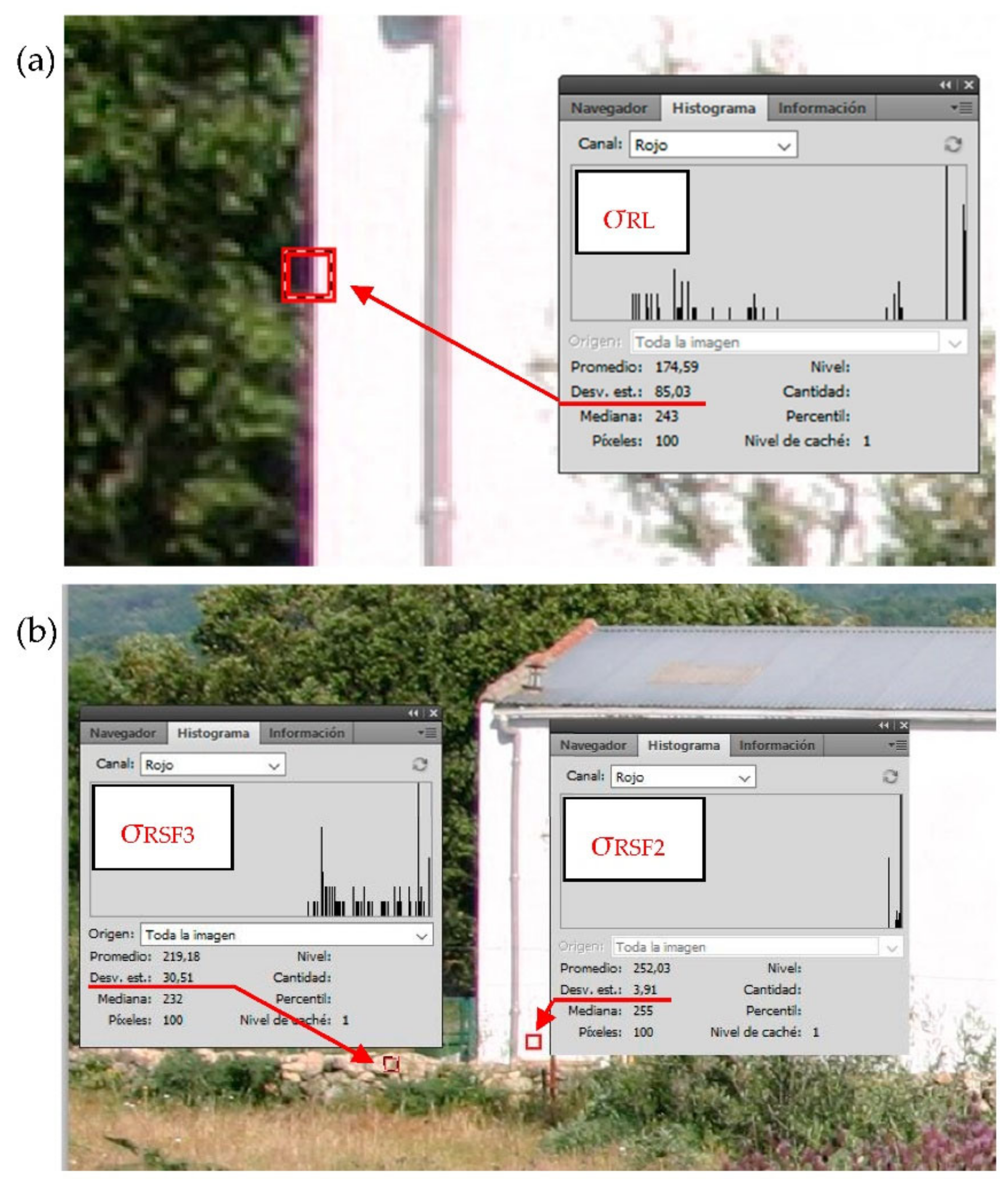
The sharpness of a border line or silhouette line is calculated by the standard deviation of the mean of the colours in the basic colour channels (σ_xi; x = R, G, B) on the boundary between the surfaces of the building and the background [11] (Figure 1a). This is performed using quadrangular sample areas containing a border line that is located between the building and the background. The resolution of this capture window of 10 × 10 pixels is, in theory, sufficient for calculating the sharpness of lines in photo resolutions of 100–150 dpi; however, photos with higher resolutions require a proportional increment in the quadrangular capture window. The number of sample areas or windows can vary, but a minimum of three must be used.

The standard deviation (SD: σ) for the red (R) (0–255), green (G) (0–255), and blue (B) (0–255) channels (σ_xi; x = R, G, B; i = 1 − n) is calculated using Adobe Photoshop (C) for each sampling area, and the arithmetic mean per colour channel is calculated for the building (Equation (1)).

$${\overline{\mathsf{\sigma }}}_{\mathrm{x}}=\frac{{{\displaystyle \sum }}_{\mathrm{i}=1}^{\mathrm{n}}{\mathsf{\sigma }}_{\mathrm{xi}}}{\mathrm{n}}$$

(1)

where x = R, G, B, and i = number of sampling areas.

Depending on the means obtained, sharpness is classified as high (SD > 40) (for any of the three channels), medium (SD 26–40), or low (SD < 26) [11].

2.2. Additional Assessment of Colour Impact (CI)

The study is complemented by an analysis of the colour of the built area, using the method for colour impact measurement which was described previously [36].

This method considers both the visual characteristics of the colours (hue, saturation, and brightness) and the internal contrast between the building and the surroundings.

Colour impact was determined by comparing the mean hue (H), saturation (S), and brightness (B) of colours between the building and the most dominant feature in the surroundings. Single main colours were selected from the walls and roofs to represent the colour of the buildings. H, S, and B are compared using selected sampling areas (10 × 10 pixels) representing the roof (SF1) or the facade (SF2) of the building, and the feature chosen in the surroundings (SF3).

The average values of H (0–360°), S (0–100%), and B (0–100%) obtained for SF1 and SF2 were then compared to the mean values recorded for SF3 by the simple subtraction of mean values between building and surrounding. As many as six comparisons between pairs were performed—three from the facade vs. three from the roof.

Comparison pairs showing high contrast were considered based on the assumption that (1) the larger the number of high-contrast HSB pairs, the greater the visual impact should be and (2) the larger the number of impact pairs attributable to the facade, the more visible the building should prove to be. Differences in hue (H) exceeding 72° were interpreted as generating high contrast (poorly compatible contrast (PCC)), and this threshold was set at 30% for differences in saturation (S) or brightness (B) [19]. When differences were between 36° and 72° in H comparisons and between 15% and 30% in S or B comparisons, there were no colour impacts (compatible contrasts (CC)). Lastly, diversity without contrast (DWC) occurs when differences fall into the range of 9–36° for H pair comparisons and into the range of 5–15% for S or B pair comparisons.

According to these earlier studies, colour impact is determined by comparing the means of hue (H), saturation (S), and brightness (B) of the colours of the building and the predominant surface or element in the surroundings, including the standard deviations of the internal contrast of the building relative to the background (

Table 2. Assessment of colour impact (CI).

Colour Impact (CI)	Comparison between Building Façade and Surroundings		Comparison between Building Roof and Surroundings		Total H/S/B Pairs with Poorly Compatible Contrast (PCC)
	Number of H/S/B Pairs with Poorly Compatible Contrast (PCC)	Internal Contrast (+)	Number of H/S/B Pairs with Poorly Compatible Contrast (PCC)	Internal Contrast (+)
(1–2) *	0	NM	0	NM	0
2	0	NM	1	↓	1
3	0	NM	1	↑≈	1
3	1	≈↓	0	NM	1
3	0	NM	2	↓	2
3	1	↓	1	↑≈↓	2
3	1	↓	2	≈↓	3
4	1	↑	0	NM	1
4	1	↑≈	1	↑≈↓	2
4	0	NM	2	↑≈	2
4	2	≈↓	0	NM	2
4	1	↑≈↓	2	↑	3
4	1	↑≈	2	≈↓	3
4	2	↓	1	↑≈↓	3
5	2	↑	0	NM	2
5	2	↑≈	1	↑≈↓	3
5	0	NM	3	↑≈↓	3
5	3	↑≈↓	0	NM	3
5	Up to 3	↑≈↓	Up to 3	↑≈↓	>3

Notes: NM—not measurable; ↑—high; ≈—medium; ↓—low. (1–2) *—comparisons between building and surroundings reach compatible contrasts (CC) or (2) diversity without contrast (DWC) (1) at most. (+)—Internal contrast is measured as the standard deviation of the central colour value (mean) and the values on the rest of the surface in the basic channels of red (R), green (G), and blue (B). Data from [36].

). Using Photoshop, it is possible to establish comparison pairs by colour channel between building surfaces (roof and façade) and the majority surface in the surroundings to classify the overall colour impact of a building. When an impact pair was established, the method was completed by measuring the internal contrast. In cases with no impact pairs, this parameter was not measured. Internal contrast was measured by comparing the standard deviation obtained for colour channels (R, G, B) within the same sampling areas used for HSB comparisons (10 × 10 pixels). Internal contrast was deemed low (↓) when differences were <5 points, medium (≈) for differences in the range of 5–15 points, and high (↑) for differences >15 points [12] (Figure 1b).

Finally, the impact was converted into a simple scale of increasing ordinal impacts from 1 to 5 (Table 2). Further details about this method of measurement are provided in studies by Montero et al. [36] and García et al. [19].

2.3. Assessment of Aggregate Impact (AI)

In formal impact assessment methods, the simple aggregate sum of partial impacts has been demonstrated to be a suitable indicator for assessing global visual impacts [25,26]. In the present study, the method proposed for assessing the aggregate impact resulting from the screening and colour variables is the simple sum of the values of ScrI and CI, as calculated in Table 1 and Table 2.

2.4. Validation of the Study

To validate the proposed method for measuring screening impact, various images were created in Photoshop and used in a survey administered to a wide range of respondents. Real photos of isolated buildings in periurban locations were selected in a study area representative of the central–western region of Spain in terms of landscape, relief, and architecture.

2.4.1. Study Area and Photo Capture

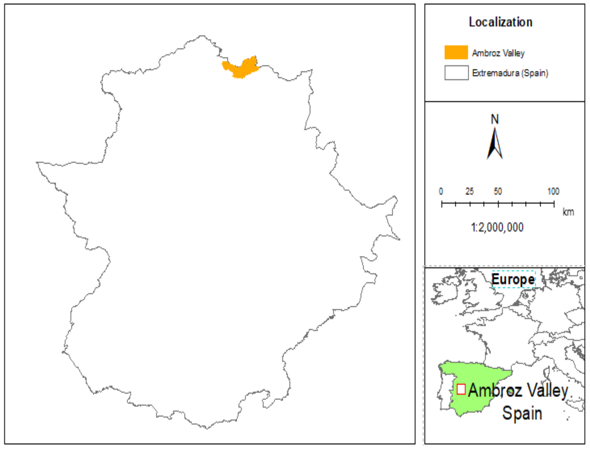
The Ambroz Valley (inland Spain: [40°15′0.4″8 W-6°01′10″8 N]) was chosen as the study area because tourism has increased in the area despite a drop in the population, among other reasons [37] (Figure 2). An inventory of new constructions was conducted by field work and using geographical information systems (GIS). Buildings that were difficult to access or were poorly visible from main roads were not included. Eight initial buildings were chosen for separate or combined analysis of the study variables: scale, colour, materials, lines, and forms. Two of these eight buildings (Figure 2 and Figure 3) were chosen for the study objectives. The selection criteria were: (1) use or type of building: agricultural or residential (the two predominant uses in the chosen area [37]); (2) location: isolated buildings in periurban areas on the side or in the bottom of valleys with a mountainous background (allowing contrast analysis); and (3) optimum visibility for photo capture.

The following guidelines applied to photo capture: (1) sufficient distance from the observer to the building so that the photos show as many details of the building as possible and part of the landscape background. In previous studies, this meant that the building occupied 25–30% of the total area of the image [38,39]. (2) Avoid taking photos in adverse weather conditions, such as rain, cloud cover, fog, or mid-day sun [40,41].

2.4.2. Generating Survey Images

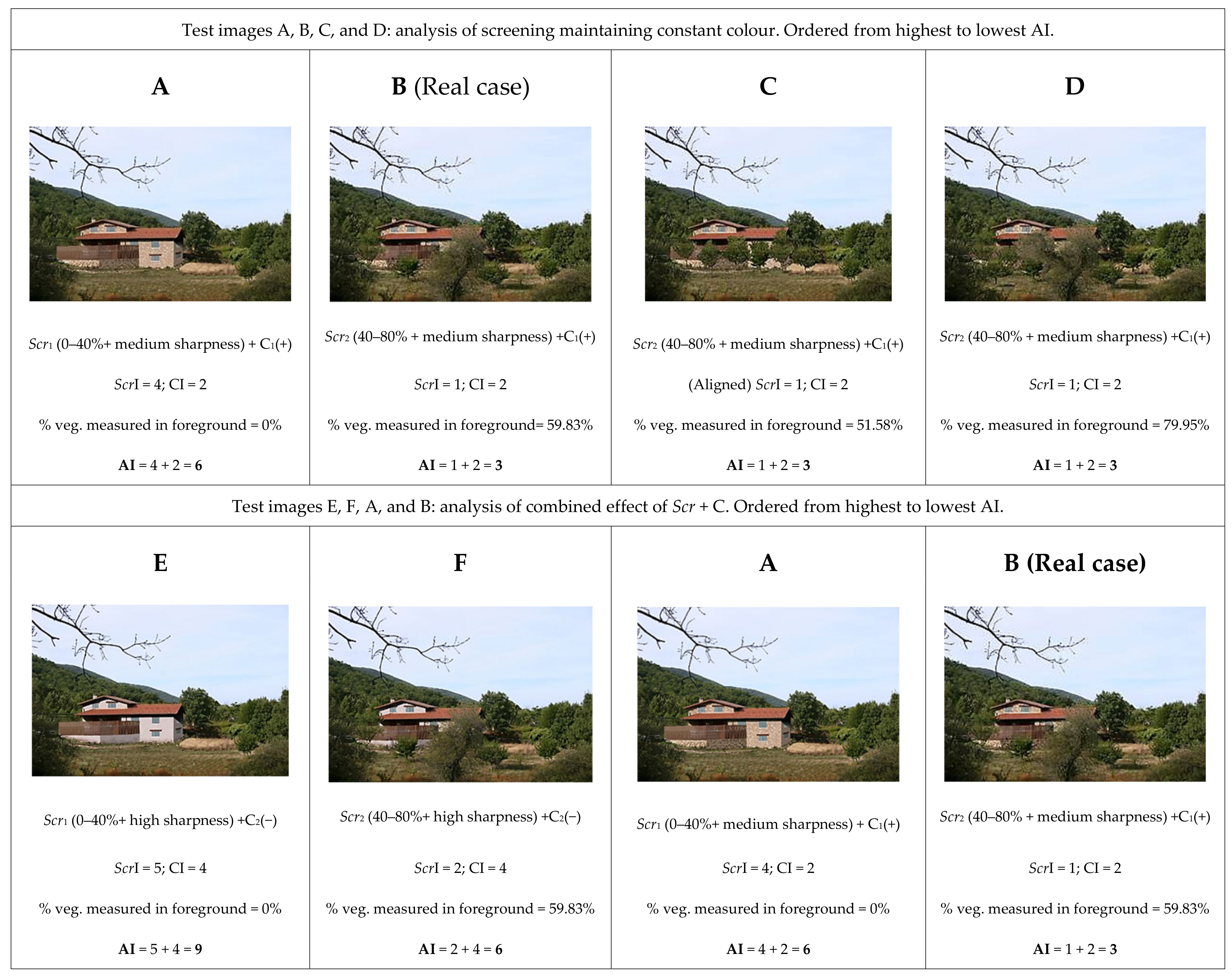
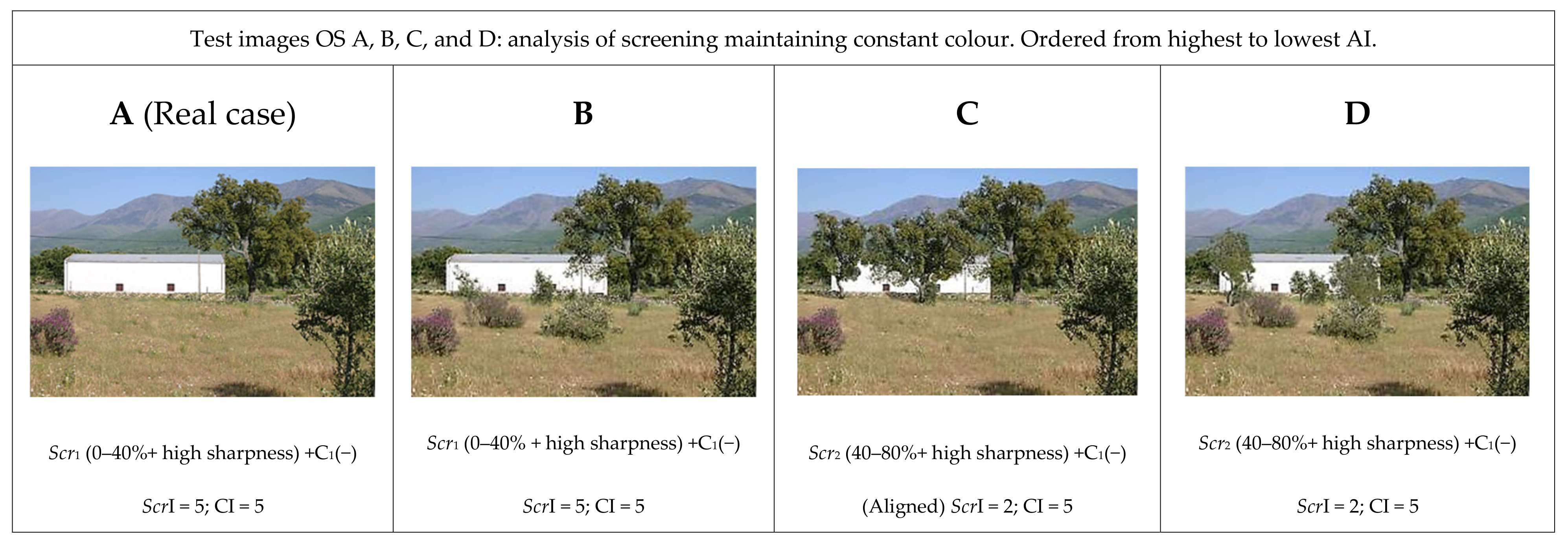
Using the two real cases chosen for the study, six survey images were proposed for each building type (residential or agricultural: cases A, B, C, D, E, and F). The images were obtained by modifying the real case using Photoshop, resulting in 12 test images for analysis: 6 residential and 6 agricultural (Figure 3 and Figure 4).

From each sequence of six images, four cases corresponded to variations in the vegetation element (Figure 3 and Figure 4, cases A–D), maintaining the original design of the initial photo and thus isolating the effect of vegetation from other variables in the statistical analysis. Adding a further element to the work completed in 2010, case C presents a configuration of aligned vegetation, included with the aim of confirming whether the arrangement of vegetation has a significant visual effect with regard to irregular configurations B and D.

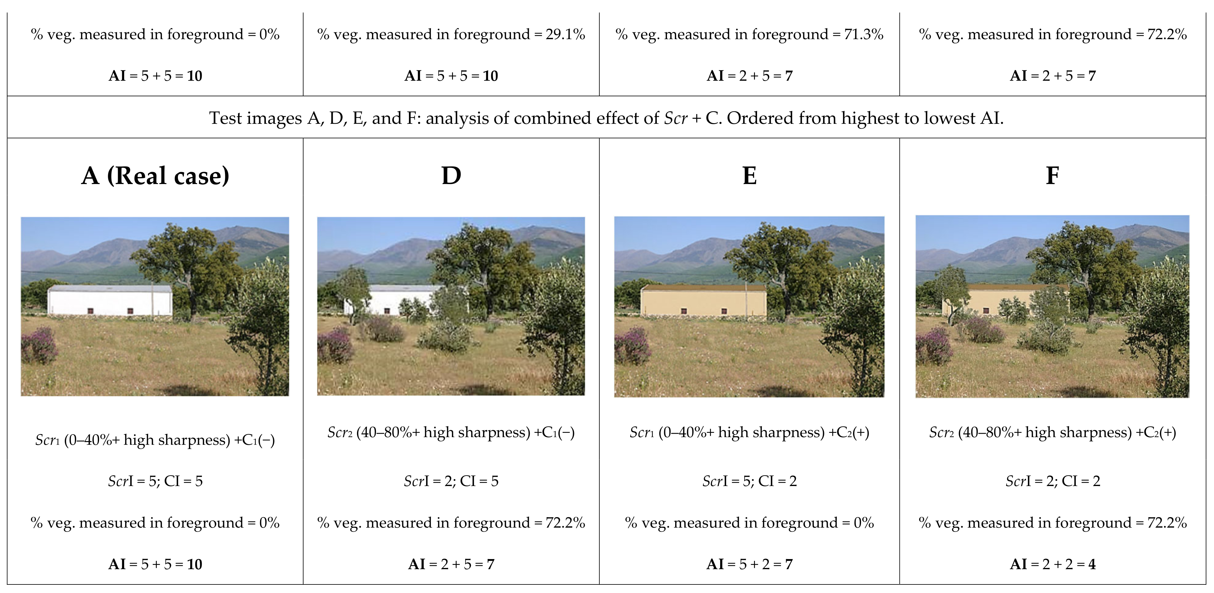
The other two images (Figure 3 and Figure 4, cases E and F) are combinations of two levels of screening, with a change in the original colour, with the purpose of analysing the possible combined effect of colour and screening. Using the 12 cases and based on Table 1 and Table 2, the impacts (CI and ScrI) and their aggregate sum (AI) were calculated before the survey was administered (Figure 3 and Figure 4).

From the remaining six initial cases, other survey images were created (32 in total) to assess the analysis of change in other variables not included in this study [36,42]. This resulted in a total of 44 (32 + 12) images to be used for the public survey.

2.4.3. Participants and Data Collection

Two separate groups of respondents took part, and two samples of 22 (16 + 6) photos each were shown per group: residential type for group 1 (Figure 3) and agricultural type for group 2 (Figure 4). This design reduced the total number of photos per respondent to a more manageable number [11] and allowed the use of independent samples to assess the influence of each test image [36]. Test images were shown to each group randomly so that the answers were not affected by the order of appearance of the images [38,43,44].

Each respondent answered two questions for each image viewed: (1) “On a scale from 1 (Very bad) to 5 (Very good), how would you rate the integration of the building into the scene?” The rating scale, with increasing ordinal numbers from 1 to 5, allowed for ongoing processing of the answers; therefore, the average rating of each image was calculated [45]. These types of rating scales are considered reliable in studies of a social nature as a simple and efficient way of measuring participants’ hedonic tone when given a visual stimulus [46]. (2) “From the following list, what would you change to improve the integration of the building into the environment? Scale of the building, Colours of the building, Construction materials, Vegetation around the building, Nothing”. Respondents could choose only one of five possible answers for question 2. The accumulated response frequencies were calculated for each image.

A total of 1046 respondents answered one of the two designed surveys. Respondents were recruited through a specially designed website. The use of web pages for this type of study—of a social nature—has been shown to be efficient for collecting answers [47]. Group 1 (residential survey) comprised 559 participants, and group 2 (agricultural survey) comprised 487 participants. Participants were sorted by age, place of residence, and gender (

Table 3. Study variables.

Variables		Categories of variables
AGE (A)		1 (≤15–25 years)
		2 (>25–55 years)
		3 (>55 years)
Place of residence (P)		1 (≤1000–10,000 inhab.)
		2 (≥10,000–500,000 inhab.)
		3 (≥500,000 inhab.)
GENDER (G)		1 (Male)
		2 (Female)
TEST IMAGE (I) Within subject	A
	B
	C
	D
	E
	F

).

2.4.4. Statistical Analysis of Results and Initial Hypotheses

The dependent study variables are the answers to the two questions asked. For question 1, the averages of the ratings per test image were used (rating average, RA), and for question 2, the accumulated frequency of the element of change most often chosen in each test image (% of element of change—EC) was used. The study factors or independent variables are shown in Table 3.

An initial analysis was conducted to determine whether the variables—gender (G), age (A), place of residence (P), and test image type (I)—affected the rating average (RA) (question 1). To this end, the following repeated-measures ANOVA test was designed: 3(A) × 3(P) × 2(G) × 6(S). The final variable (I) was a within-subject statistical analysis variable, whereas the other three (A, P, and G) were between-subject analysis variables. The statistical weight of the social variables is limited or null in the overall rating of each test image; therefore, they were not included in the main study.

Two repeated-measures ANOVA tests were performed for each building type, excluding the social variables. The independent variable was the test image type (I). The first test was intended to detect the isolated effect of screening (variable Scr, cases A–D) on the RA, whereas the second was performed to analyse the combined effects of the screening and the colour of the building on the rating (variable Scr: cases E, F, A, and B: residential (Figure 3); cases A, D, E, and F: agricultural (Figure 4)).

Significant ANOVAs were completed with post hoc analysis (Bonferroni test). Using this type of analysis, we can identify where the statistical differences were between the categories in the variable test image (I) that had significance for the answer.

Cohen’s d was used to analyse the effect size of the significant differences observed. Following methods available in the literature [48], Cohen’s d values of more than 0.8 were considered large effect sizes. The sample size in the final survey (n = 1047) was considered sufficient to detect at least medium effect sizes (Cohen’s d of more than 0.5) at significant thresholds of statistical power ((0.90 = 1 − beta; beta = 0.10); alpha = 0.01) [49].

The results of the answers to the second question were analysed using frequency diagrams and the chi-squared test for both samples surveyed.

To determine the minimum percentage of vegetation for an image with a discordant colour to receive a good rating, a logarithmic regression analysis was performed on initial cases A–D of the agricultural sample, following the cognitive theories of the W-F Law.

The statistical research hypotheses were as follows:

• According to the proposed method, within a single class of vegetation screening, the same trend would be expected in the ratings, regardless of whether the trees were in a disperse arrangement or aligned and regardless of whether the percentage of vegetation was close to the upper or lower limit of the class. To determine this, cases B, C, and D in the residential group in the same screening class (40–80%) had different percentages of vegetation (51–72%) and two screening arrangements: disperse (cases B and D) and aligned (case C). Similarly, in the agricultural sample and in class 0–40%, two proposals were presented with different percentages, A (0%) and B (30%), to determine the performance of the chosen range. The effect of the vegetation arrangement (aligned or disperse) in cases C and D of the agricultural sample (both with screening values around 70%) also helped to test the independence hypothesis in the results regarding the tree arrangement.
• According to the proposed aggregate impact method, it was expected that the sum of the two impacts would cause a decrease in the rating as the sum increased. To test this hypothesis, test images A, B, E, and F (residential) and A, D, E, and F (agricultural) were used.

3. Results

In the present study, we classified effect sizes with a Cohen’s d of 0.2 as small, those with values greater than 0.5 as medium, and those with values greater than 0.8 as high [48].

A preliminary global analysis of both samples showed that the group of respondents aged older than 55 years gave a better rating, on average, for all images than the youngest group of respondents (<25 years) and those in the middle age range (25–55 years) (data not shown); these results are similar to those obtained by Montero et al. [36]. However, the effect sizes of these results were not very high compared with the variable test image (residential: F (1552) = 7.693; p = 5 × 10⁻⁴; d = 0.33; agrarian: F (1481) = 16.010; p = 1.8 × 10⁻⁷; d = 0.52; alpha = 0.01.)

The analysis of respondents’ place of residence in relation to the agricultural sample showed that respondents from places with fewer than 10,000 inhabitants gave slightly lower ratings than the remaining respondents (data not shown); however, the effect size was also low (F (1481) = 9.397; p = 1 × 10⁻⁴; d = 0.39; alpha = 0.01). In the residential sample, the answer trend was similar but not statistically significant. The effect of gender was not significant in the answers in either sample.

Only one interaction was significant: test image type (A-F) x age; however, again, the effect size was less than 0.5 in both samples (data not shown).

The variable test image (I, within-subject analysis variable) had more statistical weight in the rating average (RA) than the social variables (between-subject analysis variables).

For both population samples, variable I (A–F) was not only significant in the within-subject analysis but also had a large effect size (residential: F (1552) = 173.069; p = 1.4 × 10⁻³⁴; d = 1.20; agricultural: F (1481) = 253.436; p = 3.8 × 10⁻⁴⁶; d = 1.452; alpha = 0.01).

In summary, only the results of the within-subject analysis are presented, in view of their greater statistical weight.

3.1. Rating of Screening

The repeated-measures ANOVA was significant and had large effect sizes in both samples (Cohen’s d = 0.741 in residential sample; Cohen’s d = 1.09 in agricultural sample) (Figure 5). Therefore, depending on the variation in screening impact (ScrI), respondents’ ratings varied significantly.

For detailed analysis of where these significant differences occurred, post hoc analysis was performed to compare test images using the Bonferroni test in both samples (Figure 5).

For the residential sample, the differences occurred only between image A (Scr = 0%; ScrI = 4) and the other three test images. The initial hypothesis of equal answers between test images with the same class of screening was also confirmed, with no significant differences between images B, C, and D (Scr = 40–80%; ScrI = 1). The hypothesis was confirmed, regardless of whether tree arrangement was dispersed (B and D) or aligned (C) and regardless of whether the percentage of vegetation was close to the upper or the lower limit of the class (Figure 5a).

Similarly, for the agricultural sample, the initial hypotheses were confirmed. Screening class 0–40% showed no significant differences between test images A and B (Scr = 0–40%; ScrI = 5), regardless of the screening percentages. There were no significant differences between cases C and D in the 40–80% class, regardless of whether the trees were in an aligned or dispersed arrangement (Scr = 40–80%; ScrI = 2) (Figure 5b).

For the agricultural sample, wherein all cases present with a high CI, a logarithmic fit was sought for approximate determination of the minimum percentage of vegetation screening required for the test images to be rated as RA = 2.5 out of 5. In this regard, 2.5 was considered the statistical midpoint value of rating averages from on ordinal scale of 1–5 used in this work. This statistical value can be used as an adequate starting point for ensuring public approval of the visual integration of buildings.

The results of this fit were calculated using Equation (2). The fit had a high R², but parameters “a” and “b” were not significant (data not shown).

The Scr% that meets the assessment rating of 2.5 points on the increasing rating scale—as predicted with this model—occurs precisely at 40%.

$$RA=\mathrm{a}·\mathrm{Ln}\left(Scr\right)+{\mathrm{b} \mathrm{R}}^2=89.4\% ; \mathrm{a}=0.426 \mathrm{b}=0.992$$

(2)

$$RA=Rating Average Scr=\% vegetation measured$$

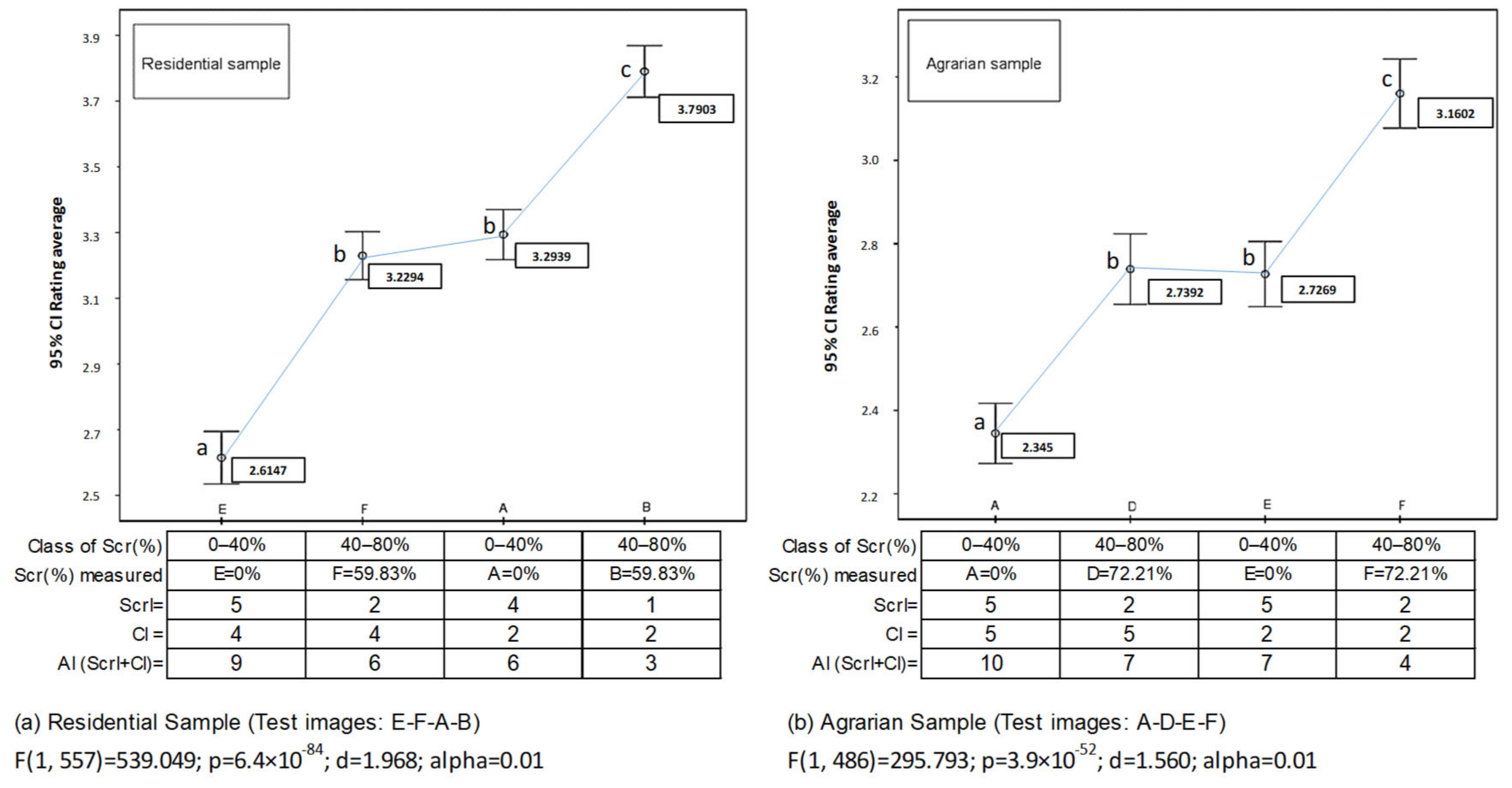
3.2. Rating of the Combined Effect of Scr × C

Analyses of test image sequences A–D–E–F (agricultural sample) and E–F–A–B (residential sample) also showed the direct influence on image rating of the aggregate sum of the impacts of both study variables: colour (C) and screening (Scr). The repeated-measures ANOVA was significant, and the effect size was large in both samples (Cohen’s d = 1.968 in residential sample; Cohen’s d = 1.560 in agricultural sample) (Figure 6). Therefore, depending on the variation in the impact in both variables (ScrI + CI), respondents’ ratings varied significantly. The Bonferroni test indicated the location of these differences between the test images in each sample, with a surprising similarity between samples (Figure 6). Overall and irrespective of the sample, the results show that the higher the sum of the impact resulting from both variables, the lower the rating will be (cases E (Figure 6a) and A (Figure 6b)) and vice versa (cases B (Figure 6a) and F (Figure 5b)). The cases of intermediate impact in both samples also had a similar response, with no significant differences between cases (Figure 6).

For both samples, a decreasing and significant linear fit was obtained between the RA and the sum of the AI (Equations (3) (residential) and (4) (agricultural)). Once again, it was clear that the higher the increase in aggregate impact, the lower the average rating. Both fits had a high R². The fitting parameters “a” and “b” were also significant in both equations (data not shown).

$$RA=\mathrm{a}-\mathrm{b}·\left(\mathrm{AI}\right){ \mathrm{R}}^2=99.2\% ; \mathrm{a}=4.408 \mathrm{b}=0.196$$

(3)

$$RA=\mathrm{a}-\mathrm{b}·\left(\mathrm{AI}\right){ \mathrm{R}}^2=99.9\% ; \mathrm{a}=3.694 \mathrm{b}=0.136$$

(4)

$$RA=\mathrm{Rating} \mathrm{Average} \mathrm{AI}=\mathrm{Aggregate} \mathrm{Impact}$$

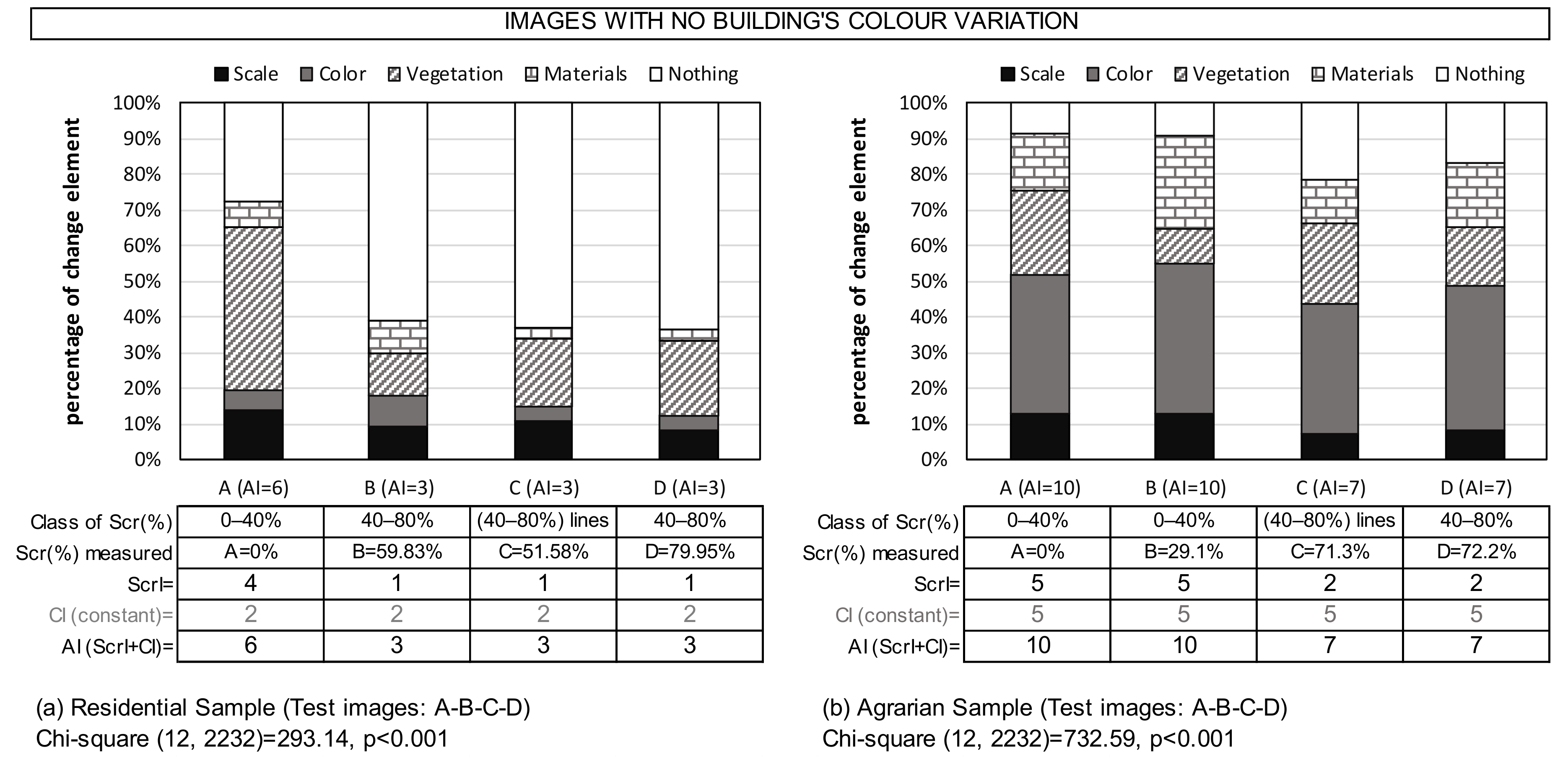
3.3. Analysis of Frequencies: Elements of Change

The answers to the second question differed between samples when comparing test images A, B, C, and D (Figure 7a,b). In the residential sample, when the percentage of vegetation increased (cases B, C, and D), selections of the option to change “nothing” increased. Moreover, these images had the lowest AI (3) and were the highest-rated. However, in case A (AI = 6), with no vegetation in the foreground, the number of answers electing to change the “surrounding vegetation” increased. Colour was rarely chosen in any of the four cases, consistent with the low CI in the sequence of cases (Figure 7a). However, for the agricultural sample, the effect of the highest CI (5) made colour the most frequently chosen element to change, irrespective of the level of screening of the building (Figure 7b).

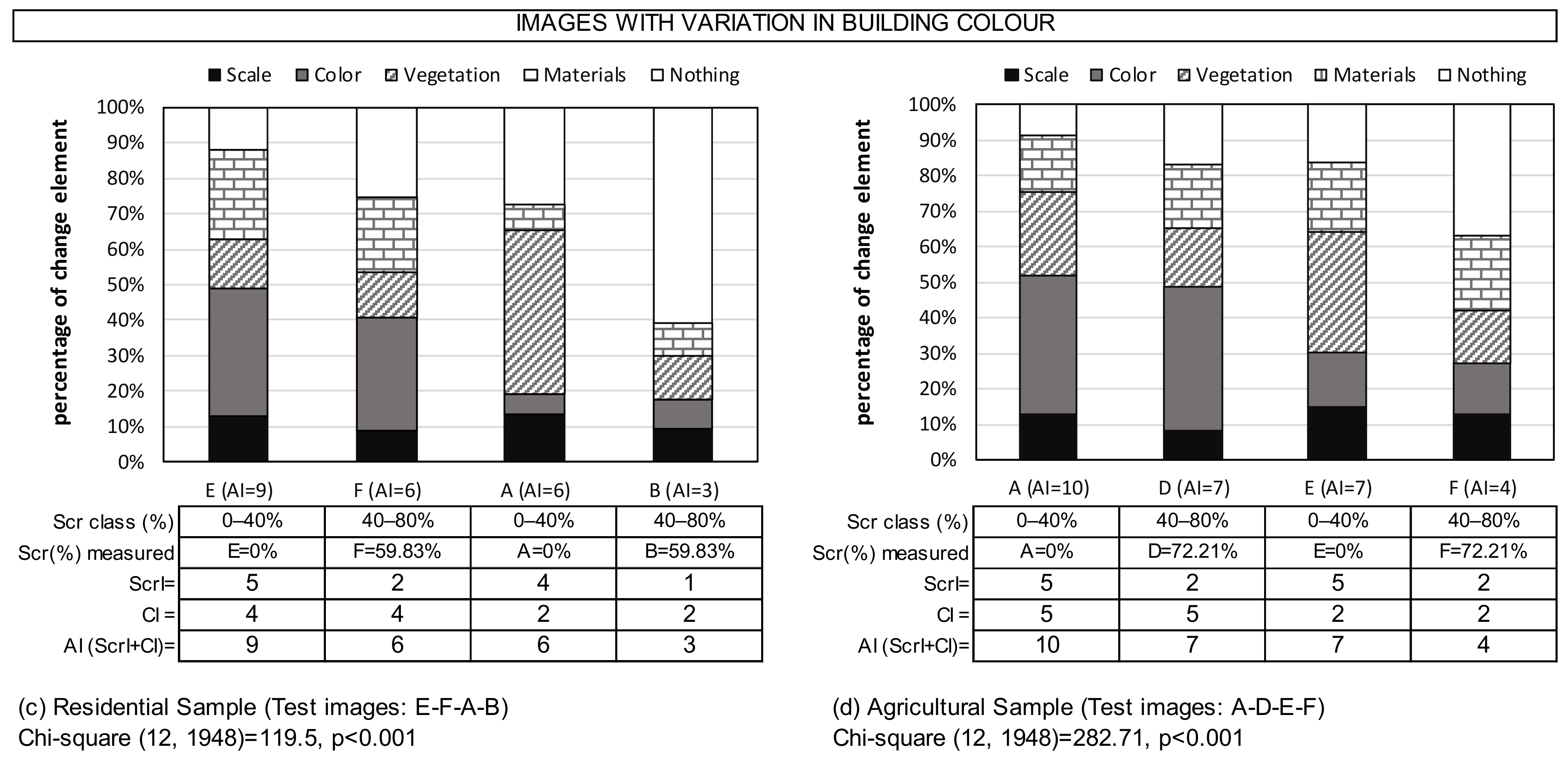
For the sequences with variation in both variables (Figure 7c,d), the effect, with a few differences, was similar in both samples. In cases of high AI (9/10), the predominant element chosen for change was colour, occurring in cases of more discordant colour and 0% screening. In cases where the AI was lower (3), the selection of the option to change “nothing” increased in both samples.

Intermediate cases with the same AI also had a similar response in the two samples. In cases F (residential) and D (agricultural), in which colour contributed more to AI, colour was the most frequently chosen element for change. In cases A (residential) and E (agricultural), the opposite occurred, with vegetation being the most frequently chosen element for change because the impact of screening in these cases contributed more to the AI.

4. Discussion

The only results included and discussed below are the within-subject results of all the respondents for test image type, which had more statistical significance and effect [36] in the preliminary ANOVA (residential d = 1.20 vs. agricultural d = 1.45). This analysis indicates that not all the images were rated the same, and the answers depended on the study variables in each test type (screening and colour).

4.1. Rating of Vegetation Screening (Test Images A, B, C, and D)

In both samples, the linear arrangement of trees showed no significant differences with dispersed arrangement in the comparison class. This shows that respondents did not visually prefer this type of arrangement to an irregular or dispersed arrangement. Similar results were obtained by Garrido et al. [39], although these authors did not quantify the percentage of vegetation used or measure its impact.

The minimum percentage of vegetation screening for a building with a dissonant colour to start to transition towards an acceptable rating is 40%, as indicated by the obtained logarithmic model (Equation (2)). The good fit of this model is encouraging and supports the W-F law; however, a more data points would be necessary to confirm this law. Nevertheless, the goodness of the obtained logarithmic fit can be understood as an initial approximation to affirm that the relationship between the increases in a percentage of a stimulus and the detection does not follow a linear trend [38,50,51,52].

The increment in the rating was significant (Bonferroni tests) in the residential cases with a shift from 0% vegetation to 50% vegetation (50% increment from case A to case C) and from 30% to 70% in the agricultural cases (40% increment from case B to case C) (Figure 5). Both graphics also show a nonlinear trend in respondents’ answers. Other authors reported that 40–50% shifts in visual stimuli [7,20,39] become appreciable for observers.

Similar results were obtained by Liang B. et al. [53], who conducted a study with photo simulations to analyse whether increasing tree cover in residential streets would have a measurable effect for an average observer. Their results suggested that to ensure an acceptable preference value (ratings of at least three on a five-point scale), cover should not be less than 41%. They also demonstrated that the relationship between tree cover and preference followed a curvilinear function rather than a linear function.

The chosen percentage of 40% between the screening classes proposed in this study therefore appears to be correct. Moreover, the recommended minimum of 40% vegetation to screen a poorly integrated design appears to be an efficient value [27].

It is clear in both samples or types that increasing the percentage of vegetation in front of a building significantly affects the rating of the building, irrespective of the colour of the façade and the roof. However, if the colours of the building are well-integrated, screening may not be necessary, as indicated by the ratings that were always higher than three in the residential sample (Figure 5a). Similar results were reported by García et al. [11].

4.2. Rating of the Combined Effect of Scr × C

The aggregate sum of impacts followed the same trend, irrespective of building type and respondent group, producing a decreasing linear relation between the aggregate sum of impacts and the rating of the images. The fits obtained in both Equations (3) and (4) were very good with regard to R² and were significant in estimating the parameters. Similar results were reported by Montero et al. [36], who supported the theory of the influence of the aggregate sum of impacts on visual perception in which the whole contributed more as a sum of parts than each part separately [54,55].

Despite this, the ratings in the residential sample never dropped to the very bad categorisation, even in the test image with the greatest impact (case E, Figure 6a). This may be due to the construction materials of both initial buildings, which clearly performed better in the residential case than in the agricultural case (case B residential, Figure 3; case A agricultural, Figure 4). In studies on the visual impact of a building based on its visual design elements, the “construction materials” study variable has been shown to have a significant contribution [11,36,44,56,57,58]. However, the impacts resulting from this aspect were not assessed or measured in this study.

Intermediate test images obtained similar ratings, with no significant differences in either sample. Both cases had the same overall total AI: six in cases F and A (residential) and seven in cases D and E (agricultural) (Figure 6). Buildings with a discordant colour that is partially screened (cases F (residential, Figure 6a) and D (agricultural, Figure 6b)) and a building with an integrated colour and no screening had the same effect on observer preference.

4.3. Analysis of Frequencies: Elements of Change

Although the increased percentage of screening in the foreground of a building had a positive effect in both samples (Figure 5a,b), in the agricultural case, the most discordant colour remained detectable and dissonant; therefore, this was the case that was most frequently identified by respondents as requiring changes (Figure 7b). The effect of colour as the most recognisable surface element in visual impact studies has been described by other authors [19,21,59]. When the colour and the overall built design of a construction are good, the average observer appears to want to add some vegetation (case A, Figure 7a). The literature includes works that showed an improvement in the visual preferences of respondents when the level of screening of a construction was partially increased with vegetation [24,25,60].

Although images with the same AI obtained similar ratings and showed no significant differences (cases F and A (residential) and D and E (agricultural); Figure 6a,b), the average observer can recognize which element has the greater impact, choosing colour or vegetation as the most common element of change according to their higher or lower contribution to the aggregate sum of impacts (Figure 7c,d). Similar results were obtained in previous studies, e.g., by Montero et al. [36] for scale and colour and by García et al. [11] for lines and forms.

5. Conclusions

The proposed method was shown to work well and was validated using surveys. The use of tree vegetation to screen the view of a building clearly improves the rating of the visual integration of the construction, regardless of whether trees are aligned or in dispersed arrangement. Moreover, 40% of vegetation screening appears to be the percentage after which the integration of a building starts to noticeably improve.

In the study of the vegetation–colour interaction, the colour of the building is the most significant element chosen for change when its impact is high or very high (impact of four or five for colour), irrespective of the level of vegetation screening. However, using tree vegetation for screening in these cases reduces the negative effect of the colour, increasing the probability of obtaining an “acceptable” rating for visual integration. Using vegetation in these cases is highly recommended, especially in cases in which the design cannot be improved.

The absence of vegetation in cases of façades with little or moderate colour impact (colour impacts 1–3) and high-quality finishings still results in acceptable levels of integration; therefore, the use of vegetation may be optional, although it is recommended wherever possible.

The transfer of the results of this research to the planning field can contribute to a more sustainable environment, facilitating policy recommendations. The proposed method is easy to use with minimal training and could be useful, especially in tourist destinations, where visual integration of buildings is a problem to be addressed.

Finally, the method can be used in similar rural areas, as the cognitive principles on which it is based do not depend on the working environment.

References

- Dentoni, V.; Grosso, B.; Massacci, G.; Cigagna, M.; Levanti, C. Numerical Evaluation of Incremental Visual Impact. In Proceedings of the 18th Symposium on Environmental Issues and Waste Management in Energy and Mineral Production, SWEMP, Santiago, Chile, 19–23 November 2018; Widzyk-Capehart, E., Hekmat, A., Singhal, R., Eds.; Springer: Cham, Switzerland, 2019. [Google Scholar]
- Antrop, M.; Van Eetvelde, V. Sensing and Experiencing the Landscape. In Landscape Perspectives; Landscape Series; Springer: Dordrecht, The Netherlands, 2017; Volume 23. [Google Scholar]
- Dupont, L.; Ooms, K.; Antrop, M.; Van Eetvelde, V. Comparing saliency maps and eye-tracking focus maps: The potential use in visual impact assessment based on landscape photographs. Landsc. Urban Plnn. 2016, 148, 17–26. [Google Scholar] [CrossRef]
- Dupont, L.; Ooms, K.; Antrop, M.; Van Eetvelde, V. Testing the validity of a saliency-based method for visual assessment of constructions in the landscape. Landsc. Urban Plan. 2017, 148, 17–26. [Google Scholar] [CrossRef]
- Guo, S.; Sun, W.; Chen, W.; Zhang, J.; Liu, P. Impact of Artificial Elements on Mountain Landscape Perception: An Eye-Tracking Study. Land 2021, 10, 1102. [Google Scholar] [CrossRef]
- Gobster, P.H.; Ribe, R.G.; Palmer, J.F. Themes and trends in visual assessment research: Introduction to the Landscape and Urban Planning special collection on the visual assessment of Landscapes. Landsc. Urban Plan. 2019, 191, 103635. [Google Scholar] [CrossRef]
- Palmer, F.P. Effect size as a basis for evaluating the acceptability of scenic impacts: Ten wind energy projects from Maine, USA. Landsc. Urban Plan. 2015, 140, 56–66. [Google Scholar] [CrossRef]
- Palmer, J. The contribution of key observation point evaluation to a scientifically rigorous approach to visual impact assess-ment. Landsc. Urban Plan. 2019, 183, 100–110. [Google Scholar] [CrossRef]
- Sun, H.; Kiang-Heng, C.; Reindl, T.; Yu Lau, S. Visual impact assessment of coloured Building-integrated photovoltaics on ret-rofitted building facades using saliency mapping. Sol. Energy 2021, 228, 643–658. [Google Scholar] [CrossRef]
- Español, I.M. Impacto ambiental. ETSI Caminos, Canales y Puertos; Universidad Politécnica: Madrid, Spain, 1995. [Google Scholar]
- García, L.; Montero, M.J.; Hernández, J.; López, S. Analysis of lines and forms in buildings to rural landscape integration. Span. J. Agric. Res. 2010, 8, 833–847. [Google Scholar] [CrossRef]
- García, L.; Hernández, J.; Ayuga, F. Analysis of the materials and exterior texture of agro-industrial buildings: A pho-to-analytical approach to landscape integration. Landsc. Urban Plann. 2006, 74, 110–124. [Google Scholar] [CrossRef]
- Grossberg, S.; Pessoa, L. Texture segregation, surface representation and figure-ground separation. Vis. Res. 1998, 38, 2657–2684. [Google Scholar] [CrossRef] [Green Version]
- Neumann, H.; Yazdanbakhsh, A.; Mingolla, E. Seeing surfaces: The brain’s vision of the world. Phys. Life Rev. 2007, 4, 189–222. [Google Scholar] [CrossRef]
- Neufert, E. Arte de Proyectar en Arquitectura; Ed Gustavo Gili: Barcelona, Spain, 1982. [Google Scholar]
- Zacharias, J. Preferences for view corridors through the urban environment. Landsc. Urban Plan. 1999, 43, 217–225. [Google Scholar] [CrossRef]
- Humphreys, G.W.; Cinel, K.; Wolfe, J.; Olson, A.; Klempen, N. Fractionating the binding process: Neuropsychological evidence distinguishing binding of form from binding of surface features. Vis. Res. 2000, 40, 1569–1596. [Google Scholar] [CrossRef]
- Vanrell, M.; Baldrich, R.; Salvatella, A.; Benavente, R.; Tous, F. Induction operators for a computational colour-texture representation. Comput. Vis. Image Underst. 2004, 94, 92–114. [Google Scholar] [CrossRef]
- García, L.; Hernández, J.; Ayuga, F. Analysis of the exterior colour of agro-industrial buildings: A computer aided approach to landscape integration. J. Env. Man. 2003, 69, 93–104. [Google Scholar] [CrossRef]
- O’Connor, Z. Façade Colour and Judgements about Building Size and Congruity. J. Urban Des. 2011, 16, 397–404. [Google Scholar] [CrossRef]
- Hernández, J.; López-Casares, S.; Montero, M.J. Análisis metodológico de la relación entre envolvente y urbanización exterior en construcciones rurales para la mejora de la integración paisajística. Inf. Construcción 2013, 65, 497–508. [Google Scholar] [CrossRef]
- Amir, S.; Gidalizon, E. Expert-based method for the evaluation of visual absorption capacity of the landscape. J. Environ. Manag. 1990, 30, 251–263. [Google Scholar] [CrossRef]
- Crow, T.; Brown, T.; De Young, R. The Riverside and Berwyn experience: Contrasts in landscape structure, perceptions of the urban landscape, and their effects on people. Landsc. Urban Plan. 2006, 75, 282–299. [Google Scholar] [CrossRef]
- Ikemy, M. The effects of mystery on preference for residential façades. J. Environ. Psychol. 2005, 25, 167–173. [Google Scholar] [CrossRef]
- Bishop, I.D.; Wherrett, J.R.; Miller, D.R. Using Image Depth Variables as Predictors of Visual Quality. Environ. Plan. B Plan. Des. 2000, 27, 865–875. [Google Scholar] [CrossRef]
- Hernández, J.; García, L.; Morán, J.; Juan, A.; Ayuga, F. Estimating visual perception of rural landscapes: The influence of vegetation, The case of Esla Valley (Spain). Food Agric. Environ. 2003, 1, 139–141. [Google Scholar]
- Jiang, L.; Kang, J.; Schroth, O. Prediction of the visual impact of motorways using GIS. Environ. Impact Assess. Rev. 2015, 55, 59–73. [Google Scholar] [CrossRef]
- Weber, E.H. De Pulsu, Resorptione, Auditu Et Tactu. In Annotationes Anatomicae et Physiologicae; Koehler: Leipzig, Germany, 1834. [Google Scholar]
- Deheaene, S. The neural basis of the Weber-Fechner law: A logarithmic mental number line. Res. Focus 2003, 7, 145–147. [Google Scholar] [CrossRef]
- Garrido Velarde, J.; Montero Parejo, M.J.; Hernández Blanco, J.; García-Moruno, L. Using Native Vegetation Screens to Lessen the Visual Impact of Rural Buildings in the Sierras de Béjar and Francia Biosphere Reserve: Case Studies and Public Survey. Sustainability 2019, 11, 2595. [Google Scholar] [CrossRef]
- Gimblett, H.R. Environmental cognition: The prediction of preference in rural Indiana. J. Archit. Plan Res. 1990, 7, 222–234. [Google Scholar]
- Lynch, J.A.; Gimblett, H.R. Perceptual values in the cultural landscape: A spatial model for assessing and mapping perceived mystery in rural environments. Comput. Environ. Urban 1992, 16, 453–471. [Google Scholar] [CrossRef]
- Stamps, A.E., III. Mystery, complexity, legibility and coherence: A meta-analysis. J. Environ. Psychol. 2004, 24, 1–16. [Google Scholar] [CrossRef]
- Gimblett, H.R.; Itami, R.M.; FitzGibbon, J.E. Mystery in an Information Processing Model of Landscape Preference. Landsc. J. 1985, 4, 87–95. [Google Scholar] [CrossRef]
- García Moruno, L. Criterios de Diseño Para la Integración de las Construcciones Rurales en el Paisaje. Ph.D. Thesis, Universidad Politécnica de Madrid, Madrid, Spain, 1998. [Google Scholar]
- Montero-Parejo, M.J.; Garcia-Moruno, L.; Lopez-Casares, S.; Hernandez-Blanco, J. Visual Impact Assessment of Colour and Scale of Buildings on the Rural Landscape. Environ. Eng. Manag. J. 2016, 15, 1537–1550. [Google Scholar] [CrossRef]
- Hernández, J.; García, L.; Montero, M.J.; Sánchez, A.; Lopez, S. Determinación de los Impactos Producidos en los Humedales de Extremadura para su Defensa y Protección Ambiental. In 204 Landscape Architecture-The Sense of Places, Models and Applications (Identifying Impacts on Wetlands of Extremadura for Environmental Protection); FAME (Fundación Alfonso Martín Escudero): Madrid, Spain, 2007; p. 196. (In Spanish) [Google Scholar]
- Garrido-Velarde, J.; Montero-Parejo, M.J.; Hernández-Blanco, J.; García-Moruno, L. Visual analysis of the height ratio between building and background vegetation. Two rural cases of study: Spain and Sweden. Sustainability 2018, 10, 1890. [Google Scholar]
- Garrido-Velarde, J.; Montero-Parejo, M.J.; Hernández-Blanco, J.; García-Moruno, L. Use of video and 3D scenario visualisation to rate vegetation screens for integrating buildings into the landscape. Sustainability 2017, 9, 1102. [Google Scholar]
- Grêt-Regamey, A.; Bishop, I.D.; Bebi, P. Predicting the scenic beauty value of mapped landscape changes in a mountainous region through the use of GIS. Environ. Plan. B Plan. Des. 2007, 34, 50–67. [Google Scholar] [CrossRef]
- Bishop, I.D. Determination of Thresholds of Visual Impact: The Case of Wind Turbines. Environ. Plan. B Plan. Des. 2002, 29, 707–718. [Google Scholar] [CrossRef]
- Montero Parejo, M.J.; Jeong, J.S.; García Moruno, L.; Hernández Blanco, J. Metodología para la cuantificación del impacto visual de materiales y detalles de fachada en edificación rural (in spanish). In Proceedings of the VIII Iberian Congress of Agro-Engineering, Orihuela, Spain, 1–3 June 2015. [Google Scholar]
- Imamoglu, Ç. Complexity, liking and familiarity, architecture and non-architecture Turkish students’ assessments of traditional and modern house facades. J. Environ. Psychol. 2000, 20, 5–16. [Google Scholar]
- Montero-Parejo, M.J.; García-Moruno, L.; Reyes-Rodríguez, A.M.; Hernández-Blanco, J.; Garrido-Velarde, J. Analysis of Façade Colour and Cost to Improve Visual Integration of Buildings in the Rural Environment. Sustainability 2020, 12, 3840. [Google Scholar] [CrossRef]
- Kendrick, J. Social Statistics: An Introduction to Using SPSS, 2nd ed.; Allyn and Bacon: Boston, MA, USA, 2005. [Google Scholar]
- Nasar, J.L. Adult viewers’ preferences in residential scenes: A study of the relationship of the environmental attributes to preference. Environ. Behav. 1983, 15, 589–614. [Google Scholar] [CrossRef]
- Roth, M. Validating the use of Internet survey techniques in visual landscape assessment—An empirical study from Germany. Landsc. Urban Plan. 2006, 78, 179–192. [Google Scholar] [CrossRef]
- Stamps, A.E. A paradigm for distinguishing significant from non significant visual impacts: Theory, implementation, case histories. Environ. Impact Assess Rev. 1997, 17, 249–293. [Google Scholar] [CrossRef]
- Rosenthal, R.; Rosnow, R.L. Essentials of Behavioral Research: Methods and Data Analysis, 2nd ed.; McGraw Hill: New York, NY, USA, 1991. [Google Scholar]
- Varela, M. Évaluation Pseudo–Subjective de la Qualité d’un Flux Multimédia. Ph.D. Thesis, University of Rennes 1, Rennes, France, 2007. [Google Scholar]
- Nasar, J.L.; Stamps, A.E., III. Infill McMansions: Style and the psychophysics of size. J. Environ. Psychol. 2009, 29, 110–123. [Google Scholar] [CrossRef]
- Reichl, P.; Egger, S.; Schatz, R.; D’Alconzo, A. The logarithmic nature of QoE and the Role of theWeber-Fechner Law in QoE assessment. In Proceedings of the 2010 IEEE International Conference on Communications, Cape Town, South Africa, 23–27 May 2010. [Google Scholar]
- Jiang, B.; Larsen, L.; Deal, B.; Sullivan, W.C. A dose–response curve describing the relationship between tree cover density and landscape preference. Landsc. Urban Plan. 2015, 139, 16–25. [Google Scholar] [CrossRef]
- Cañas, I.; Ayuga, E.; Ayuga, F. A contribution to the assessment of scenic quality of landscapes base don preferences expresed by the public. Land Use Policy 2009, 26, 1173–1181. [Google Scholar]
- Smardon, R.C.; Palmer, J.F.; Felleman, J.P. Foundations for Visual Project Analysis; John Wiley: New York, NY, USA, 1986; Available online: www.esf.edu/es/via (accessed on 1 March 2022).
- Stamps, A.E., III. Physical Determinants of Preferences for Residential Facades. Environ. Behav. 1999, 31, 723–751. [Google Scholar] [CrossRef]
- Akalin, A.; Yildirim, K.; Wilson, C.; Kilicoglu, O. Architecture and engineering students’ evaluations of house façades: Pref-erence, complexity and impressiveness. J. Environ. Psychol. 2009, 29, 124–132. [Google Scholar]
- Montero-Parejo, M.J.; Jeong Su, J.; Hernández-Blanco, J.; García-Moruno, L. Rural Landscape Architecture: Traditional ver-sus Modern Façade Designs inWestern Spain. In Landscape Architecture; The Sence of Places, Models and Applications; Intechopen: London, UK, 2018. [Google Scholar]
- Shang, H.; Bishop, I.D. Visual Thresholds for detection, recognition and visual in landscape settings. J. Environ. Psychol. 2000, 20, 125–140. [Google Scholar]
- Tveit, M.; Ode, A.; Fry, G. Key Concepts in a Framework for Analysing Visual Landscape Character. Landsc. Res. 2006, 31, 229–255. [Google Scholar]