
The Impact of Fine-Scale Present and Historical Land Cover on Plant Diversity in Central European National Parks with Heterogeneous Landscapes


1
South Moravian Museum in Znojmo, Přemyslovců 8, 66902 Znojmo, Czech Republic
2
Silva Tarouca Research Institute for Landscape and Horticulture, Lidická 25/27, 60200 Brno, Czech Republic
*
Author to whom correspondence should be addressed.
Land 2022, 11(6), 814; https://doi.org/10.3390/land11060814
Submission received: 20 April 2022
/
Revised: 24 May 2022
/
Accepted: 25 May 2022
/
Published: 31 May 2022
(This article belongs to the Special Issue Conservation of Bio- and Geo-Diversity and Landscape Changes)
Abstract
:As the human population grows, the transformation of landscapes for human uses increases. In recent homogeneous and predominantly agricultural landscapes, land-cover and management changes are considered the main drivers of vascular plant diversity. However, the specific effects of land-cover classes across whole heterogeneous landscapes are still insufficiently explored. Here, we investigated two floristic surveys realised in 1997 and 2021, accompanied by fine-scale land-cover classes detected in 1950, 1999 and 2018, to reveal the impact of historical and present land cover on the pattern of species composition and species richness in the bilateral Podyjí and Thayatal National Parks. Multi-dimensional analyses revealed that the species composition was driven by the fine-scale historical land cover, the overall species richness was mostly affected by the river phenomenon and the present richness was mostly affected by increased soil nutrients. In well-preserved protected areas, it is especially desirable to restore disappearing land-cover classes with traditional or compensatory management to retain plant species richness, which is a key factor of biodiversity. However, management plans should also take into account the increasing amount of nitrogen in soils from long-term continual deposition, which can strongly impact the species richness, even in national parks with low current deposition.
1. Introduction
In central Europe, humans have affected landscapes and plant diversity since the Neolithic times [1]. However, with growing populations and the consequent pressure on land use, this impact has steadily increased over time [2,3]. This pressure has been most pronounced during the past two hundred years, after the modern agricultural revolution and industrial revolution at the end of the 18th and beginning of the 19th century [4] that introduced, among others, new crops, new agricultural systems, mechanisation and artificial fertilisation [5]. Besides food, the growing population also demanded more space for living, resulting in the spread of settlements and the accompanying transportation infrastructure [6]. While more fertile regions started to be overexploited over this period, less fertile and accessible regions, typically mountainous regions, started to be abandoned, mainly leading to the spread of forest [2,3]. The land overexploitation of fertile regions and abandonment of mountainous regions accelerated after the Second World War in western parts of Europe, connected with the so-called productivist agriculture and market economies [5], while in eastern parts of Europe, the introduction of the so-called socialist agriculture, connected with forced collectivisation, were the main drivers [7]. Both types were characterised by the heavy use of fertilisers, pesticides and mechanisation, leading to the loss and fragmentation of traditionally managed habitats [8]. Therefore, the long historical land-use/cover continuity in large areas was greatly disrupted, leading to homogenisation and sharp declines in biodiversity [6]. Indeed, many studies showed that regions with continuous land-cover and/or traditional land-use management enable the accumulation of many species at specific individual sites and can contribute to reducing the chance of random extinctions of rare species [9,10,11]. Such regions are usually protected and harbour one of the most species-rich plant communities, e.g., Bílé Karpaty (White Carpathian) Mts. in the Czech Republic [12,13,14,15].
However, historical continuity is only one of the factors influencing the diversity of plant communities. Diversity naturally varies across landscapes, with environmental factors, such as precipitation, soil pH, nutrient and light availability; biomass productivity [16,17,18,19]; and geological diversity causing some regions to have unusually high diversity and others to be much poorer. In addition, high topographic and meso-climatic diversity [20] can also affect patterns of species diversity, as well as alien plant invasions [21]. Both topographic and meso-climatic diversity may be even more accentuated in deep river valleys, where they are known as a ‘river phenomenon’ [22]. Nevertheless, the main drivers of species composition and species richness are considered to be land-use and management changes (in connection with historical continuity), which affect not only predominantly lowland agricultural landscapes [11,23] and settlements [24] but also mountain regions [25,26]. In general, land-cover studies have usually focused on only one type of habitat, such as grasslands [11,24] and forests [6,27], in landscapes with relatively homogeneous environmental conditions. They have generally confirmed that the combined historical and current land use is reflected in current patterns of diversity [28]. A few studies have investigated more than one land-cover category, e.g., open rural habitats [24]. A study by Michalcová [10] found that the land-cover diversity of the whole landscape contributes to between-site similarities in species composition, with the co-occurrence of many species increasing the species richness. However, complex studies of fine-scale land-cover classes at a regional scale in heterogeneous landscapes are still lacking.
In this study, we focused on two aspects of the relationships between fine-scale land-cover history and plant diversity at a regional scale in two central European national parks. First, we examined spatial heterogeneity and compared two types of landscapes with distinctive geomorphological features: a deep river valley and surrounding rather flat plains. Second, we focused on all types of habitats in the studied landscape. Our analyses, therefore, aimed to answer the following questions: (1) How does fine-scale land cover influence plant species composition in naturally well-preserved areas with long-term human impacts, but with very distinctive geomorphologies? (2) Is the species composition dependent on present or rather historical land cover? (3) Which types of land cover and relevant landscape heterogeneity indicators are important for current species richness compared with more than twenty years ago?
2. Materials and Methods
2.1. Study Area
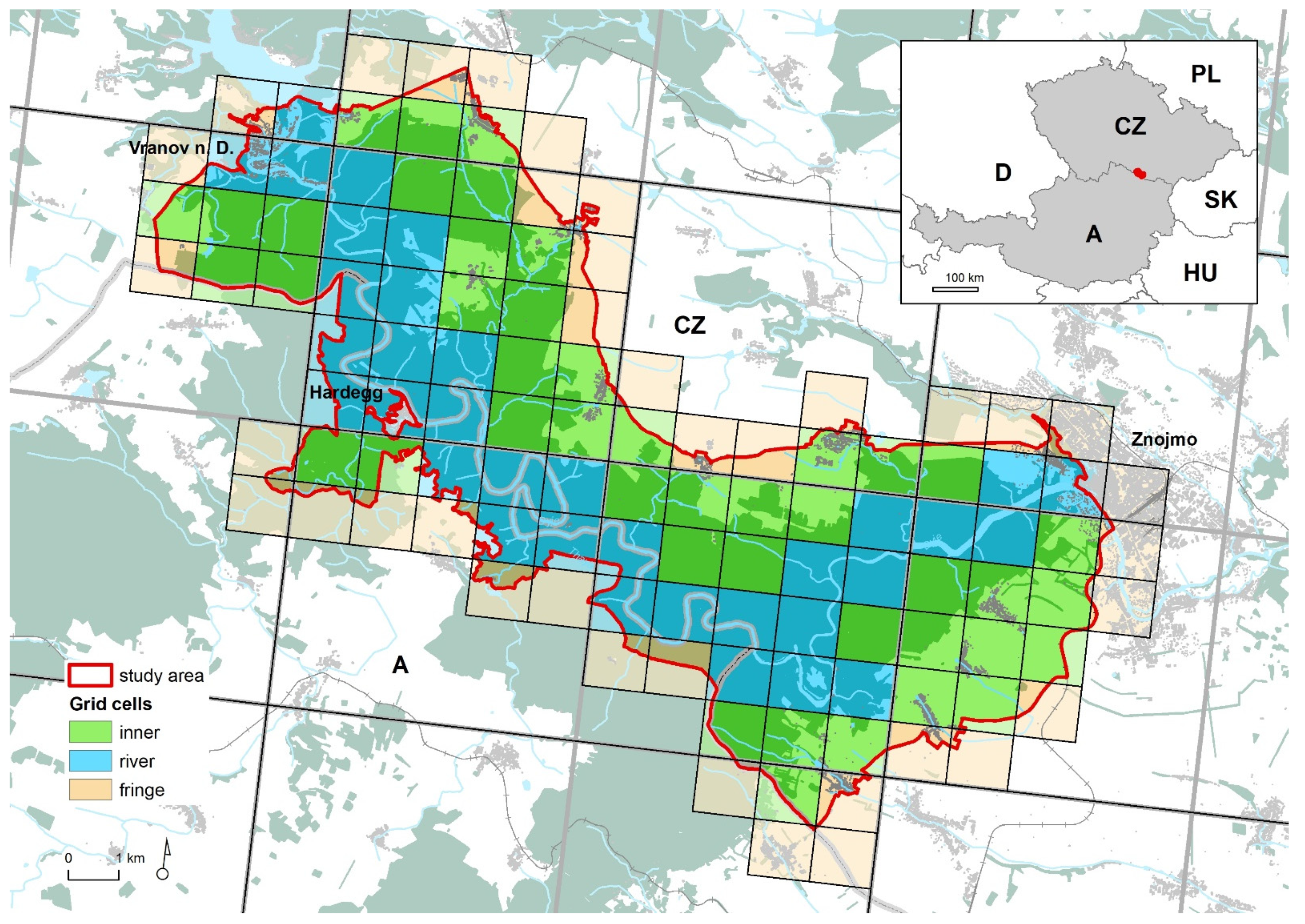
This study was performed in the bilateral Podyjí and Thayatal National Parks (NPs) and buffer zone of the Podyjí NP, situated between the towns of Vranov nad Dyjí (48°54′ N, 15°49′ E) and Znojmo (48°52′ N, 16°03′ E) along the state border between the Czech Republic and Austria (Figure 1). The total area is 105 km2, with NP Podyjí covering 63 km2, Thayatal NP covering 13 km2 and the Podyjí NP buffer zone covering 29 km2. A protected landscape area on the Czech side was declared in 1978 and was then transformed into a national park in 1991. On the Austrian side of the Dyje (Thaya) river, a national park was declared in 2000. The main part of the protected areas is formed by the river Dyje, which flows through a deep valley with varied morphology [29] and a diverse mosaic of habitats on slopes of different aspects [22]. The Dyje valley is surrounded by more or less flat relief of adjacent plateaus. The altitudinal range is from 210 m a.s.l. (river Dyje in Znojmo) to 536 m a.s.l. (Býčí hora hill near Vranov n. D.), and the maximum valley depth is almost 200 m. From a geological perspective, the crystalline bedrock of the Bohemian massif is mainly formed by gneiss, schist and granite, with restricted occurrences of crystalline limestone [30]. The eastern part of the study area is filled with Neogene sediments and the plateaus are covered by loess. Other Quaternary sediments can be found in the Dyje river and many stream valleys.
The study area is classified as a warm and dry region, with an average yearly temperature between 8 and 9 °C, mean annual precipitation of 550–600 mm and a distinct NW–SE gradient from a moderately warm to warm climate [31]. The area is located in the transition zone between the Hercynian and Pannonian floristic regions [32] and, therefore, has a significant proportion of thermophilous and continental species [22]. These varied environmental conditions have also been accompanied by specific human impacts, including the location along the so-called Iron Curtain in the second half of the 20th century, characterised by restricted movement along the Czech–German and Czech–Austrian borders. Therefore, the study area can be considered a biodiversity hotspot [33,34,35], with 1555 historically recorded species of vascular plants [36], i.e., much more species than the individual national parks in adjacent Austria (e.g., the area richest in species is the Hohe Tauern harbour with 1077 species, [37]).
The Podyjí and Thayatal NPs and their surroundings have been continuously inhabited since 5000–6000 BC [38,39,40,41,42]. For more than 800 years, mainly before the industrial revolution in the 19th century, human impacts were reflected in deforestation, pasture, burning, litter raking and coppicing [43], as well as in the cultivation of slope terraces for wine production. After the industrial revolution and the population explosion in the 19th century, anthropogenic pressure spread to the non-forested, agricultural landscape. This was accomplished by using more efficient tillage systems and the introduction of fertilisers in the 19th century and by agricultural mechanisation, the use of pesticides and fungicides, and land consolidation in the 20th century [5]. These practices have completely changed the landscape configuration and contributed to its degradation, especially in the intensively used agricultural surroundings of both national parks. While forests significantly dominated in Thayatal NP for at least the last 200 years, Podyjí NP was characterised by quite a large proportion of open landscape (24–35%) with permanent grassland and later arable land between the 1840s and 1930s, though forests have dominated since the second half of the 20th century. In contrast, the Podyjí NP buffer zone has been characterised by a greater variety in the form of vineyards, orchards, grasslands and settlements, and forests were (and still are) quite scarce [44]. Long-term continuity of forests and grasslands based on topographic maps has shown that nearly 50% of forests in the NP were preserved over the last 200 years, while less than 1% of grasslands were preserved [44].
2.2. Vascular Plant, Land Cover and Supplementary Data
Our data set consisted of a floristic grid cell survey of vascular plants conducted in two periods: 1992–1993 (first floristic survey; [45]) and 2019–2020 (second floristic survey; [36]). The grid used was derived from the grid of Central European floristic mapping by dividing the area into basic grid cells that are 1’ × 0.6’ (1.2 × 1.1 km) in size. Accordingly, the study area comprised 115 grid cells, with each cell containing a list of vascular plant taxa. The standardised methodology was applied with one exception. While during the first floristic survey, plant data were collected for the whole grid cell, regardless of the borders of the study area, during the second floristic survey, plant data were collected only for parts of the grid cell lying inside the study area. The nomenclature of plant taxa follows Kaplan et al. [46], where some hybrids or records identified only at the genus level were removed. The resulting data set included 1412 species, which is still higher than in individual Austrian National Parks (see above, [37]).
We assessed the land cover based on aerial photos, orthophotos and other digital sources in three time steps: 1954–1955 (pixel resolution 0.5 m), 1999–2001 (pixel resolution 0.2 m) and 2018–1019 (pixel resolution 0.2 m). Other digital sources were in a vector format and included agricultural data from the Land Parcel Information System (from 2020); digital cadastre data (from 2020); biotope mapping (from 2013); and settlements, roads, railroads and watercourses from the Fundamental Base of Geographic Data on the Czech Republic (from 2020). Roads, railroads and watercourses were transformed to polygon layers by buffering them with preset criteria (first-class roads 22 m wide, second-class roads 12 m, third-class roads 10 m, paved roads and streets 6 m, unpaved roads and railroads 4 m, watercourses 2 m). For the Czech part of the study area, we combined the vector data and used the result as a basis for the present state, which was adjusted and classified with the help of orthophotos from 2018–2019 [44]. We derived the present land cover in the vector format for the Austrian part by vectorizing each orthophoto. The minimum mapping unit was set to 50 m2, but in the case of settlement areas, it was lowered to 15 m2 in order to capture individual buildings. We verified the resulting land-cover layer vector in the field and adjusted it accordingly. Then, we used the present land-cover layer vector as a source for the 1999–2001 layer, where the boundaries of individual polygons were adjusted via backward editing [5] and reclassified according to the relevant orthophoto. We derived the land cover for the 1954–1955 layer via the same procedure, using the 1999–2001 layer as a basis. However, since the orthophoto from 1954–1955 had a coarser resolution, some features, namely, settlements and, to some degree, small agricultural plots, were characterized. The land-cover layers in the following text are referred to as the 1950s (from period 1954–1955), 1990s (from period 1999–2001) and present (from period 2018–2020).
In total, we distinguished 30 land-cover classes. They included forest (closed canopy woody vegetation); sparse forest (open canopy woody vegetation, characterized according to [47] as a forest with trees or shrubs 15–40 m apart); clearings (including shrubs and forest nurseries); grass-forb (grassland with scattered trees); meadows (including pastures); fallow land (land not cultivated for at least two years); natural bare surfaces (mainly rocks); natural water bodies (in the form of pools); artificial water bodies; streams; swamps (wetlands); smallholdings; small orchards (<1 ha); small vineyards (<1 ha); vineyards with trees, arable fields with trees; small arable fields (<1 ha); large orchards (>1 ha); large vineyards (>1 ha); large arable fields (1–30 ha); very large arable fields (giant) (>30 ha); gardens; public greenery; recreational areas; mining areas; waste dumps; residential built-up areas (with public buildings); industrial, agricultural and commercial areas; and roads and railroads. Two land-cover classes (natural water bodies and railroads) were omitted from the analyses due to their negligible areas.
For the land-cover analysis, for each grid cell, we calculated the proportion of land-cover classes from the three periods. We also calculated the number of patches for each grid cell, which served as the landscape heterogeneity indicator.
As supplementary variables, we used five characteristics derived from maps that could probably influence the species richness or species composition: the area belonging to Podyjí National Park (NP), the area of the Podyjí NP buffer zone, the area belonging to Thayatal NP, the area of unchanged land cover and the geological diversity. The last was computed as the Shannon diversity index based on the proportions of bedrock types from Geologische Karte der Republik Österreich 1:50,000, sheet Retz [48]. The geological diversity was counted for each grid cell, with original bedrock types merged into seven broader categories (gneiss, granite, schist, calcareous rocks, neogene sediments, loess, other Quaternary sediments). Further, we used the number and characteristics of alien plant species according to Pyšek et al. [49] and the total number of all four (C1–C4) categories of endangered species and the number of critically endangered (C1) and endangered (C2) species evaluated using The Red List of vascular plants of the Czech Republic [50]. Based on the species composition we computed mean Ellenberg indicator values calibrated for the Czech flora (EIVs; light, temperature, moisture, soil reaction, nutrients; [51]).
2.3. Statistical Analyses
To address question 1, first, we had to calculate the Bray–Curtis dissimilarity for the land cover and the Sörensen dissimilarity for floristic presence/absence data. Then, the composition and changes in land cover and floristic data were explored using the following analyses: (1) principal coordinates analysis (PCoA) embedded mentioned dissimilarities and were combined with the Hellinger distance (supplementary variables were tested using the multiple regression with 999 permutations (p < 0.001), and Ellenberg indicator values were tested using the modified permutation test according to Zelený et Schaffers [52]), (2) permutational multivariate analysis of variance using distance matrices (PERMANOVA) [53,54] and (3) multivariate homogeneity of the groups’ dispersions (PERMDISP) [54,55]. Further, the floristic beta diversity between particular surveys was computed as the Sörensen dissimilarity.
To address questions 1 and 3, changes in species richness, alien species, neophytes, EIVs and beta diversity were displayed in boxplots and analysed using parametric pairwise or unpaired t-tests accordingly, while changes in individual classes of land cover (used as relative area, i.e., percentages of the whole grid cell) were assessed using the non-parametric Friedman test (if p < 0.001, then analysis with post hoc Wilcoxon pair rank-sum tests with Bonferroni correction followed). Further changes in land-cover heterogeneity were evaluated using ANOVA repeated measures analysis (if p < 0.001, then analysis with Tukey’s post hoc tests followed) and changes in the proportions of unchanged land were analysed using the non-parametric Wilcoxon rank-sum test.
To address question 2, but also necessary for question 1 to reveal the limit value of included/surveyed grid cells area, which shows the similar pattern of species richness as the whole area of grid cells, and to identify the major land-cover classes influencing the species richness, we performed an analysis of regression trees based on the CART concept (classification and regression trees [56]; libraries rpart and rpart.plot [57]). First, we used the species richness per grid cell recorded during the second floristic survey as a dependent variable, while the proportions of each land-cover class detected in the second floristic survey, included/surveyed area of grid cells, landscape heterogeneity and proportions of individual NPs and the buffer zone were used as explanatory variables.
The regression trees based on the second floristic survey specified a limit value of 72 ha (53%) of the surveyed grid cell area (see Section 3), with grid cells surveyed in a larger area that was comparable in species richness to grid cells surveyed in the whole area. For subsequent analyses, we also divided the whole number of grid cells (n = 115) into three groups: (1) fringe cells (n = 37 for the second floristic survey, while n = 32 for the first floristic survey since five fringe cells were not surveyed) comprising grid cells on the border of the study area with smaller surveyed areas; and other cells (n = 78), which were separated into (2) inner cells (n = 44), within which the flow of the Dyje river is not present, and (3) river cells around and including the Dyje river (n = 34). Then, using regression trees, we analysed the corresponding data from the first floristic survey, examining only the inner and river cells (n = 78) according to another survey methodology. To better understand the environmental patterns, we then performed another regression tree with the addition of mean Ellenberg indicator values among the explanatory variables for the first and second surveys separately. All four trees were pruned according to expert knowledge into a maximum of eight leaf nodes.
To address questions 1 and 2, i.e., to examine the impact of the fine-scale land cover of three time periods on vegetation composition, we first classified grid cells based on the land-cover data. The proportions of 28 land-cover types were square-rooted and the Bray–Curtis dissimilarity was computed; then, the beta-flexible method (β = −0.25) was used to create three distinctive groups. Such a classification was performed on land-cover data from all periods, while the classification from the 1950s land cover was displayed on floristic data in the principal coordinates analysis (PCoA; Sörensen dissimilarity, Hellinger distance). The impact of these land-cover classifications, together with the landscape heterogeneity and geomorphology coupled with the meso-climate (river phenomenon), on species composition was tested using distance-based redundancy analysis (db-RDA; Sörensen dissimilarity, Hellinger distance). Because the high geological diversity of the Podyjí and Thayatal NPs could also affect the species richness and the species composition [10,22,30], we included this diversity in the db-RDA as a covariate to remove its impact. First, we calculated the significance and adjusted the R2 of the whole model, and then used a forward selection method appropriate for particular variable testing in db-RDA.
3. Results
The PERMANOVA analysis showed that the land cover significantly differed (p < 0.001) between the 1950s and 1990s within both the inner and river cells, while there was no significant difference between the 1990s and the present (Table 1). No difference in land cover was found within fringe cells. At the same time, the PERMDISP analysis revealed no changes in the overall landscape diversity between the examined periods.
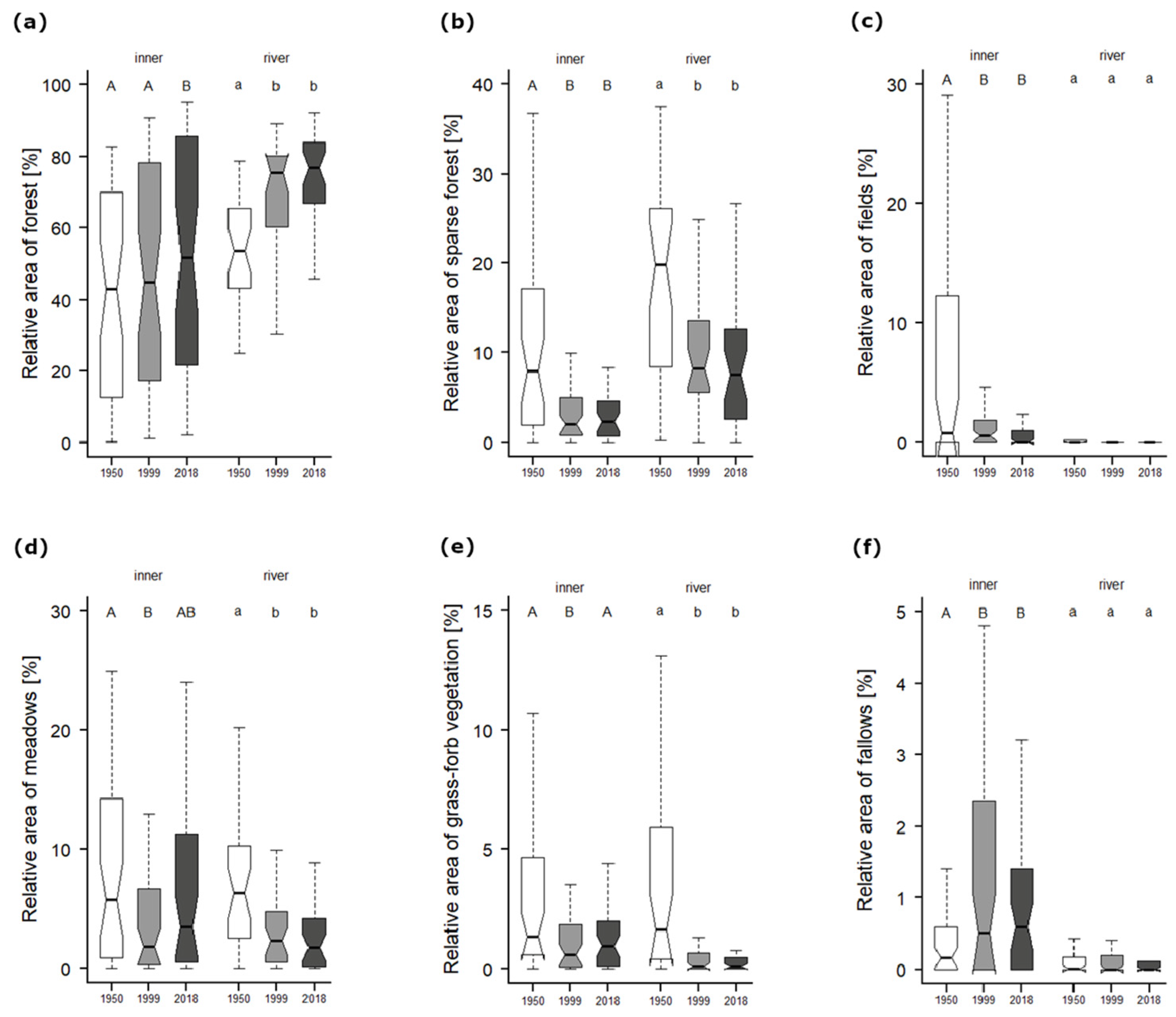
The large shift in land cover between the 1950s and 1990s (Figure A1) was clear, especially in the huge decrease in sparse forest (Figure 2b), meadow (Figure 2d) and grass-forb vegetation (Figure 2e) within both the inner and river cells; in contrast, there was an increase in fallow land (Figure 2f) within inner cells and closed canopy forest within river cells (Figure 2a). Another significant decrease was documented in inner cells within orchards, vineyards with trees, fields with trees and small fields (<1 ha; Figure 2c); in contrast, there was an increase in gardens and giant fields (>30 ha).
The same analyses for floristic data revealed a significant difference in the species composition of inner (p < 0.001) and river (p = 0.002) cells between the first and second floristic surveys, as well as in the gamma diversity of inner cells (p < 0.03), which was not significant in river cells (Table 1).
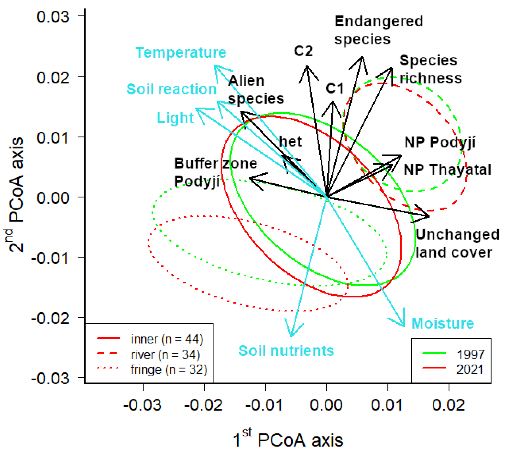
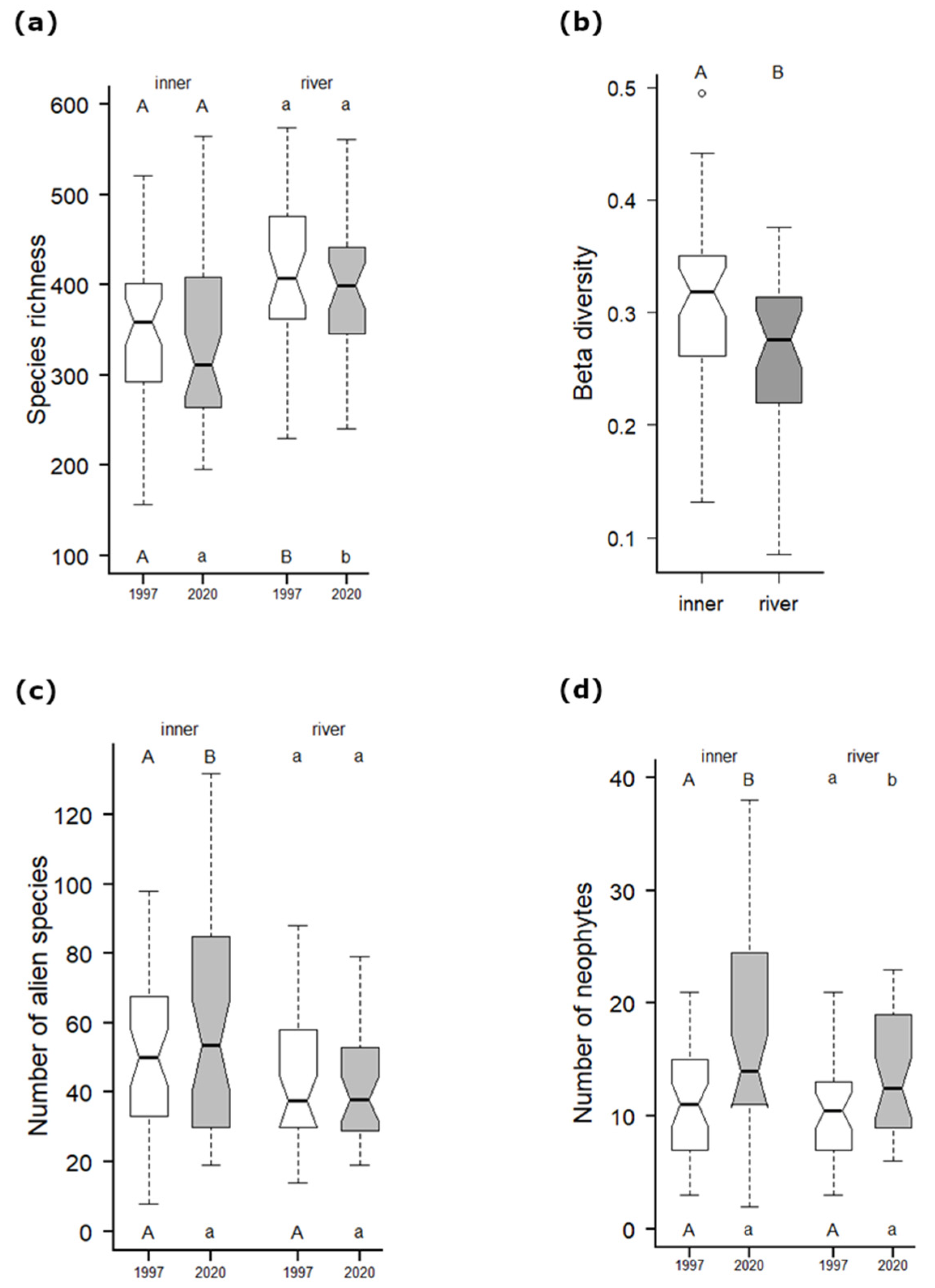
The PCoA analysis of species composition with regressed supplementary variables (Figure 3) showed a slow decrease in the species richness of both inner and river cells (but according to the pairwise t-test, the differences within these groups were not significant, Figure 4a), and there was a decrease in the light conditions (Figure A2b). Conversely, we found an increase in soil nutrients within both inner and river cells (EIV for nutrients; Figure A2a), while river cells showed an obvious shift to higher moisture conditions. Fringe cells revealed an increase in soil nutrients. The beta diversity comparing both surveys was significantly higher within inner cells (Figure 4b).
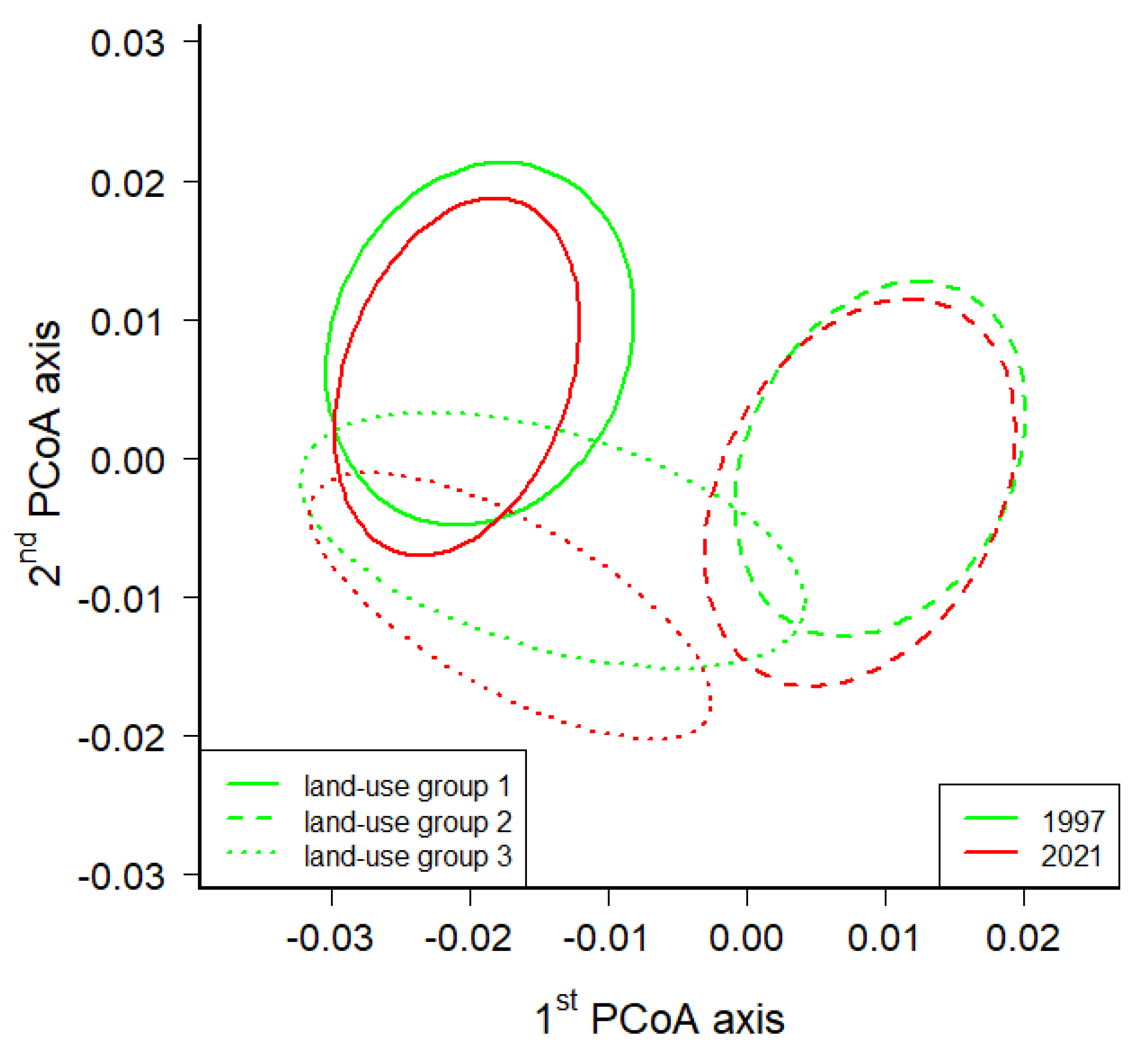
The impact on the species composition in the study area showed a similar pattern in both examined floristic surveys (Table 2). The highest impact was caused by the historical land cover (identified in the previous period; Table 1 and Figure 5), followed by the river phenomenon (geomorphology combined with meso-climate) and present land cover. In contrast, the landscape heterogeneity (Figure A2c) was not significant, and the land cover of the 1950s applied to the second floristic survey had only a negligible impact (under 1% of the explained variability).
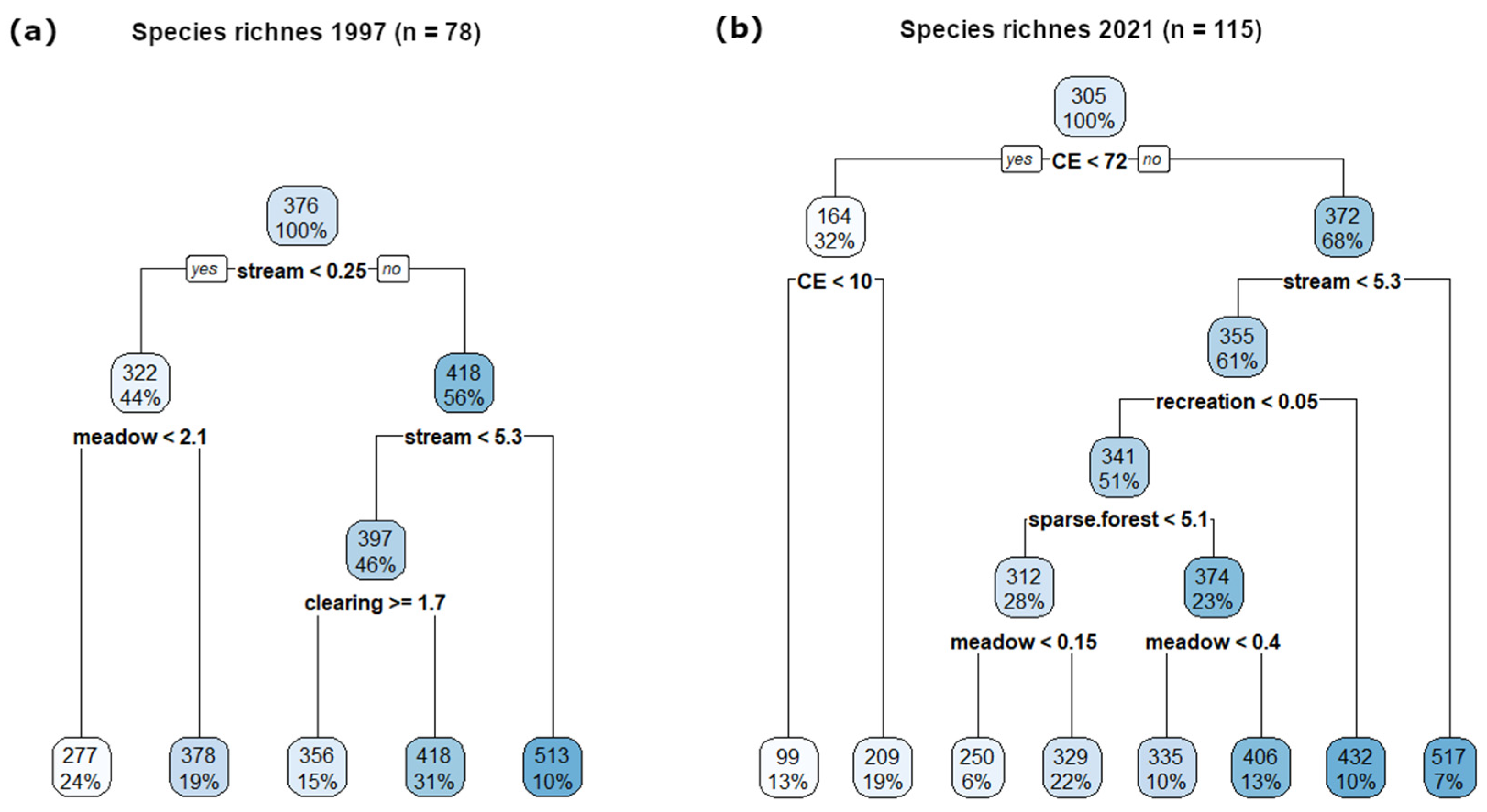
Among the present land-cover classes, the most important for species richness was streams, i.e., those grid cells including parts of the Dyje river (Figure 6b). This was followed by recreation, then sparse forest and meadows. Similarly, in the first floristic survey, the major impact on species richness was caused by streams (Figure 6a), which was also an important variable in the secondary branch level, together with meadows (Figure 6a; only 78 grid cells analysed; see Section 2.3).
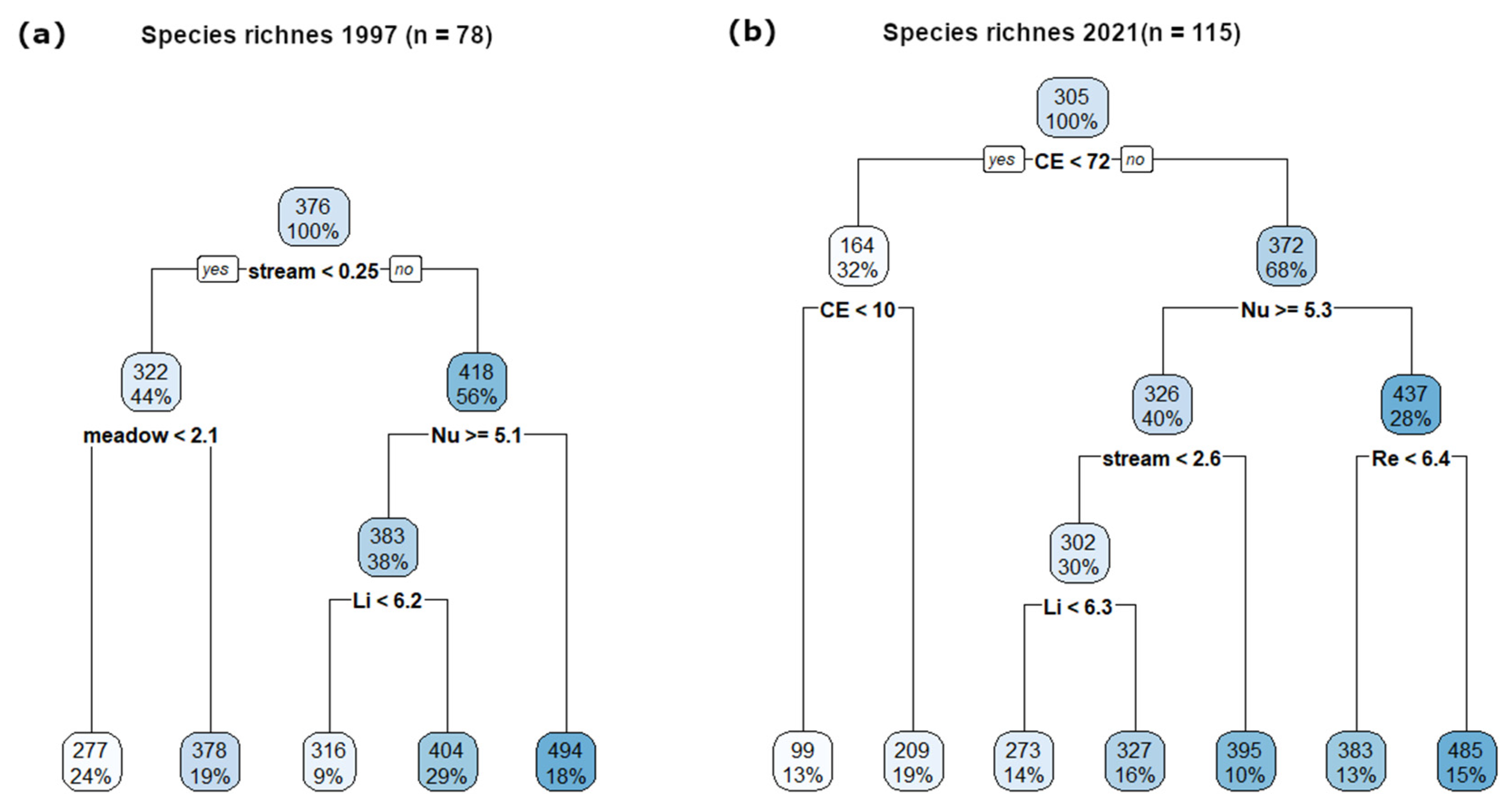
When adding the Ellenberg indicator values (EIVs) to the explanatory variables (Figure 7b), the lower content of nutrients (EIV for nutrients) was the most important for species richness in the second floristic survey, while the next node level comprised both the stream and EIVs for soil reaction (the most species-rich grid cells had a higher value of EIV for soil reaction). The EIV for light was also important. Similarly, when adding the EIVs into the first floristic survey analysis (Figure 7a), the major impact remained from streams, while in the secondary branch level, both meadows and lower EIVs for nutrients were important. Again, the EIV for light was also important.
4. Discussion
Our analyses might seem to have been led by partitioning based on the different beta diversity patterns (Figure 4b) and geomorphology into (1) river cells characterised by high geomorphological and meso-climatic diversity [21] (river phenomenon) accompanied by a diverse mosaic of habitats on slopes with different aspects, and (2) inner cells representing mainly gently undulating landscape with settlement accompanied by a rich mosaic of land cover, including rare heathlands, resulting in high plant diversity ([64]; Figure 3). However, the strong river phenomenon described in the studied area [22] and documented in our analyses (Figure 4a, Figure 6 and Figure 7) did not result in major impacts on species composition (Table 1). The major impact on species composition was found to be due to the historical land cover (Table 1 and Figure 5). This effect of historical land-cover continuity was demonstrated mainly for traditionally managed grasslands [9,11,65]. However, continually used grasslands (between 1840 and 2018) in the study area covered only 0.6%. Therefore, any separate effect of grassland continuity in our study area would be rather weak. This is different from, e.g., the White Carpathians, where continual meadows cover 3.8% of their area. On small plot sizes, these meadows are the most species-rich in the world [12,13]. On the other hand, forest continuity was found in 47.5% of our study area, and therefore, might be considered to have a strong impact, as it influences the species richness and composition mainly through the dispersal limitation of many forest specialists [66]. It should be stressed that our study reflected the land-cover composition of the whole landscape because our analyses included fine-scale information on land cover with 28 categories and their classification resulted in robust partitions (Figure 5). In both analysed floristic surveys, the historical land cover explained more variability than the cover in the respective period of the floristic survey, even though roughly 20 years (in the first survey) or even 40 years (in the second survey) had passed. This corresponded in particular with the overgrowing and abandonment of some habitat types because vegetation generally responds with some delay [67,68] and some species specialists may still survive there. Moreover, the transformation into new habitats could also permit the persistence of some species from the original habitats. These new habitats include (1) near-natural land covers inside settlements, e.g., public greenery, some managed road verges or some recreation areas [24], or (2) near-natural land covers outside settlements [6].
The main driver of species richness in the study area in both surveys was found to be the river phenomenon (Figure 6a,b), which was likely caused by sharp environmental gradients within relatively small areas [22]. The species richness was also strongly influenced by meadow areas in both surveys, although the area of historically continuous meadows (1840–2018) was very low compared with other well-preserved natural areas (e.g., White Carpathians, see above). However, these fragments still represent valuable biodiversity hotspots [29] that are important for the maintenance of species richness [24]. This is true even though the meadows within river cells declined in 1999 and continued to decline until the present, while meadows within inner cells have been partly restored (Figure 2d). In the second floristic survey, the recreation land-cover area was also important for species richness. This finding was the major difference between the two surveys and was partly due to an increase in alien species near settlements (inner cells; Figure 4c), especially escapes of cultivated plants (e.g., Muscari armeniacum, Tulipa gesneriana, Primula vulgaris, Rudbeckia hirta, Lunaria annua) in combination with the perseverance of some rare weeds (e.g., Asperugo procumbens, Chenopodium vulvaria, Urtica urens), and the occurrence of disturbed surfaces harbouring some rare endangered species (e.g., Trifolium retusum, T. striatum, Filago germanica). Another important land cover that was distinguished in the second floristic survey was the sparse forest area (Figure 2b), which still harbours some rare species of historically continually managed forests ([69]; the majority of unchanged land cover, Figure A2d). These sparse forests represent just remnants of species-rich traditionally managed forests [43], which were gradually abandoned, like in many other parts of Europe [8] until the establishment of the so-called Iron Curtain (the restricted military area on the state border, 1951–1990). This led to the total isolation of the river valley and adjacent areas and resulted in a huge decrease in sparse forests, as well as meadows and grass-forb vegetation within both river and inner grid cells (Figure 2b,d,e). Whereas sparse forests in river cells (Figure 2b) closed their canopy (;with the exception of habitats on extreme slopes with shallow soil) and meadows with grass-forb vegetation were mostly overgrown by forests (Figure 2a), inner cells were only partly abandoned (increasing of fallows, Figure 2d–f) and accessible/open areas of highly productive and easily accessible plains [26] were mostly transformed into giant fields (>30 ha; [44]). Between 1999 and 2018, the forest abandonment and canopy closing within river cells substantially slowed down, but significantly increased in settlement surroundings (inner cells; Figure 2a,b and Figure A2b). Our results, therefore, showed that the loss of the historical state of dynamic equilibrium between traditional management and natural dynamics was followed by abandonment, similar to the adjacent area of Lower Austria [70], and later by some regeneration processes, which reduced ecological complexity at the landscape scale [6] and negatively affected biodiversity (Figure 3).
When we included environmental characteristics in the form of Ellenberg indicator values (EIVs), the major driver of species richness in the first survey was still the river phenomenon (Figure 7a). Additional important variables were represented by meadows and nutrients. Meadows were important outside the river valley because grassland specialist species are rare in agricultural [24] and forested landscapes. On the other hand, nutrients played a big role in the river valley, where the most species-rich grid cells contained lower nutrients. This was typical, especially for grid cells with the majority of grassland and wetland species pools [16]. Within the nutrient-rich river cells containing fewer grassland and wetland species, light availability was likely decisive in limiting the richness of forest species [18,71]. The second survey analysis showed a substantial shift, with the nutrients content (EIV) becoming the major driver of species richness, while the river phenomenon dropped into the second branch, together with soil reaction (Figure 7b). It is alarming that the availability of nutrients (the C:N ratio was a proxy for calibrated EIVs; [51]) became the major species richness driver, even in the bilateral Podyjí and Thayatal NPs, where N deposition is one of the lowest in the whole Czech Republic [72]. These findings are nonetheless in agreement with Gallego-Zamorano et al. [73], who found a considerable impact of N deposition on species richness in some regions of Europe. Their findings also show that Europe is currently the most impacted continent, with an average decline in species richness of 34% caused by a combination of land-cover changes and N deposition, despite the trend of decreasing N deposition in Europe (for about the last 30 years; [74]). However, influences of N deposition are not easy to disentangle because of strong linkages to abandonment within the landscape scale since N deposition accelerates overgrowing. The negative N deposition impact on species richness in the Podyjí/Thayatal NPs was documented by the decline of heathlands and acidic dry grasslands [75]. Their occurrence is conditioned by nutrient limitations [76] and their species richness decline was observed across Europe [77]. Although nutrient availability (EIV) increased in both the inner and river grid cells (Figure A2a), the grid cell species richness did not significantly decrease (Figure 4a), despite indications of a declining trend (Figure 3). This could have been caused by a combination of the increase in neophytes in both inner and river cells (Figure 4d), appropriate conservation management and several biodiversity hotspots with well-buffered soils of high pH (Figure 7b). In such hotspots, the N-deposition-driven decline of sensitive species can be slow and additional species might even colonise them [78]. The well-buffered high-pH soils are also responsible for the fact that the most species-rich grid cells in the second survey are those with lower nutrient content and higher soil reaction (Figure 7b). In nutrient-rich grid cells mostly outside the river valley, light availability is likely important in determining species richness (see above; Figure 7b).
5. Conclusions
We found that in a heterogeneous landscape, historical land cover had the largest impact on species composition. At the same time, the effect of historical land cover was higher than the present land cover; therefore, we can expect that the present land cover will affect the species composition in the near future.
The species richness was driven by the river phenomenon more than 20 years ago and also at present, even though the landscape around settlements in the protected areas was under stronger human impact than in the river valley and resulted in a rich mosaic of land covers supporting species richness. Some near-natural land-cover classes with appropriate management could harbour and ease the spread of many valuable native species. Enlarging their area of occurrence is important for preventing genetic corrosion and partly substitute for overgrowing and the loss of their original habitats. On the other hand, many endangered species are very limited in their spread and are closely connected to unique localities with a continuous history, and thus, require appropriate protection and management.
Especially in well-preserved protected areas, it is desirable to restore disappearing land-cover classes with traditional or compensatory management to retain their plant species richness, which is mostly a key factor to preserve biodiversity. However, management plans should take into account the increasing amount of nitrogen in soil derived from long-term continual deposition because, combined with land-cover changes, it has a negative impact on species richness. It is necessary to highlight that soil nutrients strongly affect the species richness, even in NPs with low current N deposition, because the effects of long-term human impacts through land use/cover and N deposition are not only restricted to local scales but also operate mostly on regional and even global scales.
Author Contributions
Conceptualization—R.N., H.S. and M.V.; methodology—M.V. and R.N.; data collection of vascular plants (1997, 2021)—R.N.; analyses—M.V. and R.N.; map visualization—R.N.; paper writing—M.V., R.N. and H.S.; review and editing—R.N. and H.S. All authors have read and agreed to the published version of the manuscript.
Funding
This paper was prepared with support from the Síťové mapování cévnatých rostlin NP Podyjí/Thayatal (ConNat ATCZ045 v Programu INTERREG V-A Rakousko—Česká republika) at the Silva Tarouca Research Institute for Landscape and Horticulture with the help of Technological Agency of the Czech Republic (grant no. SS02030018—Centre for Landscape and Biodiversity).
Institutional Review Board Statement
Not applicable.
Informed Consent Statement
Not applicable.
Data Availability Statement
Not applicable.
Acknowledgments
The authors would like to thank Petr Filippov, Martin Musil, Zuzana Němcová, Radomír Řepka and the anonymous reviewers who have made significant contributions to the quality of the paper.
Conflicts of Interest
The authors declare no conflict of interest.
Appendix A
Figure A1.
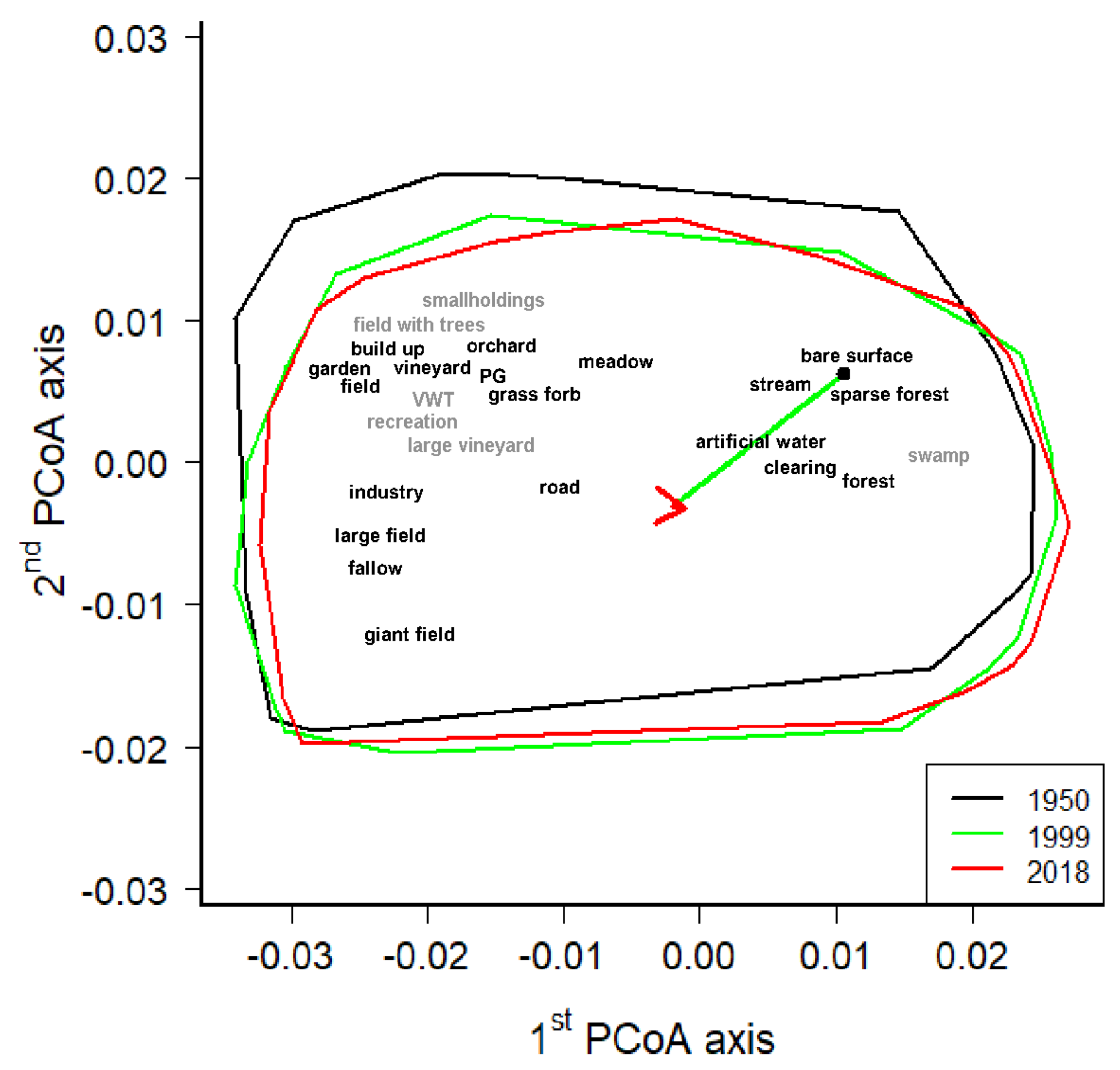
The principal coordinates analysis (PCoA) of land-cover data (proportions were square-rooted and the Bray–Curtis dissimilarity and Hellinger distance used) of all 115 grid cells in the Podyjí/Thayatal NPs detected in the years 1950, 1999 and 2018. Envelopes were drawn around the marginal grid cells in the PCoA diagram. The coloured arrow shows the shift of land-cover medoids between the searched years (1950, 1999 and 2018). Individual land covers are projected as weighted averages; grey coloured land covers occurred in less than 30 grid cells; VWT—vineyards with trees, PG—public greenery.
Figure A1.
The principal coordinates analysis (PCoA) of land-cover data (proportions were square-rooted and the Bray–Curtis dissimilarity and Hellinger distance used) of all 115 grid cells in the Podyjí/Thayatal NPs detected in the years 1950, 1999 and 2018. Envelopes were drawn around the marginal grid cells in the PCoA diagram. The coloured arrow shows the shift of land-cover medoids between the searched years (1950, 1999 and 2018). Individual land covers are projected as weighted averages; grey coloured land covers occurred in less than 30 grid cells; VWT—vineyards with trees, PG—public greenery.

Figure A2.
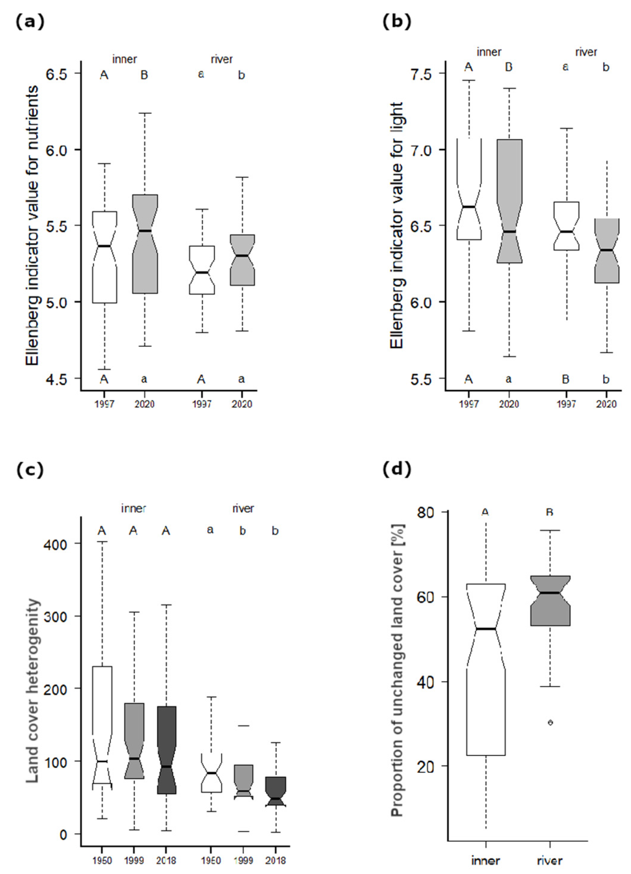
Changes and differences in the (a) Ellenberg indicator value (EIV) for nutrients, (b) EIV for light, (c) land-cover heterogeneity and (d) proportions of unchanged land cover (1950–2018) per grid cell within both the first (1997) and the second floristic survey (2021); or three land-cover searched periods (1950, 1999 and 2018) separated into inner (n = 44) and river (n = 34) group cells (see Methods). The letters above boxes (in (a) and (b)) indicate the results of pairwise t-tests between surveys within each group, while the letters below boxes show the results of non-pair t-tests between the groups. However, the letters above the land-cover heterogeneity boxes (c) show results based on the Friedman test, and when significant (p < 0.001), the post hoc Wilcoxon pairwise test with a Bonferroni correction (p < 0.01) was applied for the three periods: 1950, 1999 and 2018. Differences between proportions of unchanged land cover (d) were assessed using ANOVA repeated measures analysis (if p < 0.001, then Tukey’s post hoc tests followed). Whiskers indicate the non-outlier range with the median as the middle; boxes represent 25–75% percentiles.
Figure A2.
Changes and differences in the (a) Ellenberg indicator value (EIV) for nutrients, (b) EIV for light, (c) land-cover heterogeneity and (d) proportions of unchanged land cover (1950–2018) per grid cell within both the first (1997) and the second floristic survey (2021); or three land-cover searched periods (1950, 1999 and 2018) separated into inner (n = 44) and river (n = 34) group cells (see Methods). The letters above boxes (in (a) and (b)) indicate the results of pairwise t-tests between surveys within each group, while the letters below boxes show the results of non-pair t-tests between the groups. However, the letters above the land-cover heterogeneity boxes (c) show results based on the Friedman test, and when significant (p < 0.001), the post hoc Wilcoxon pairwise test with a Bonferroni correction (p < 0.01) was applied for the three periods: 1950, 1999 and 2018. Differences between proportions of unchanged land cover (d) were assessed using ANOVA repeated measures analysis (if p < 0.001, then Tukey’s post hoc tests followed). Whiskers indicate the non-outlier range with the median as the middle; boxes represent 25–75% percentiles.

References
- Magyari, E.K.; Chapman, J.; Fairbairn, A.S.; Francis, M.; Guzman, M. Neolithic human impact on the landscapes of North-East Hungary inferred from pollen and settlement records. Veg. Hist. Archaeobotany 2012, 21, 279–302. [Google Scholar] [CrossRef] [Green Version]
- Dahlström, A.; Cousins, S.A.O.; Eriksson, O. The history (1620–2006) of land use, people and livestock, and the relationship to present plant species diversity in a rural landscape in Sweden. Environ. Hist. 2006, 12, 191–212. [Google Scholar] [CrossRef]
- Vives, G.S.; Miras, Y.; Riera, S.; Julia, R.; Allée, P.; Orengo, H.; Paradis-Grenouillet, S.; Palet, J.P. Tracing the land use history and vegetation dynamics in the Mont Lozere (Massif Central, France) during the last 2000 years: The interdisciplinary study case of Countrasts peat bog. Quart. Int. 2014, 353, 123–129. [Google Scholar] [CrossRef] [Green Version]
- Berglund, B.E.; Gaillard, M.J.; Björkman, L.; Persson, T. Long-term changes in floristic diversity in southern Sweden: Palynological richness, vegetation dynamics and land-use. Veg. Hist. Archaeobotany 2008, 17, 573–583. [Google Scholar] [CrossRef]
- Skokanová, H.; Havlíček, M.; Unar, P.; Janík, D.; Šimeček, K. Changes of Ortolan Bunting (Emberiza hortulana L.) habitats and implications for the species presence in SE Moravia, Czech Republic. Pol. J. Ecol. 2016, 64, 98–112. [Google Scholar]
- Amici, V.; Landi, S.; Frascaroli, F.; Rocchini, D.; Santi, E.; Chiarucci, A. Anthropogenic drivers of plant diversity: Perspective on land use change in a dynamic cultural landscape. Biodivers. Conserv. 2015, 24, 3185–3199. [Google Scholar] [CrossRef]
- Bezák, P.; Petrovič, F. Agriculture, landscape, biodiversity: Scenarios and stakeholder perceptions in the Poloniny National Park (NE Slovakia). Ekológia Bratisl. 2006, 25, 82–93. [Google Scholar]
- Hejcman, M.; Hejcmanová, P.; Pavlů, V.; Beneš, J. Origin and history of grasslands in Central Europe—A review. Grass Forage Sci. 2013, 68, 345–363. [Google Scholar] [CrossRef]
- Hájková, P.; Roleček, J.; Hájek, M.; Horsák, M.; Fajmon, K.; Polák, M.; Jamrichová, E. Prehistoric origin of extremely species-rich semi-dry grasslands in the Bílé Karpaty Mts. Preslia 2011, 83, 185–204. [Google Scholar]
- Michalcová, D.; Chytrý, M.; Pechanec, V.; Hájek, O.; Jongepier, J.W.; Danihelka, J.; Grulich, V.; Šumberová, K.; Preislerová, Z.; Ghisla, A.; et al. High plant diversity of grasslands in a landscape context: A comparison of contrasting regions in Central Europe. Folia Geobot. 2014, 49, 117–135. [Google Scholar] [CrossRef]
- Johansson, L.J.; Hall, K.; Prentice, H.C.; Ihse, M.; Reitalu, T.; Sykes, M.T.; Kindström, M. Semi-natural grassland continuity, long-term land-use change and plant species richness in an agricultural landscape on Öland, Sweden. Landsc. Urban Plan. 2008, 84, 200–211. [Google Scholar] [CrossRef]
- Wilson, J.B.; Peet, R.K.; Dengler, J.; Pärtel, M. Plant species richness: The world records. J. Veg. Sci. 2012, 23, 796–802. [Google Scholar] [CrossRef]
- Chytrý, M.; Dražil, T.; Hájek, M.; Kalníková, V.; Preislerová, Z.; Šibík, J.; Ujházy, K.; Axmanová, I.; Bernátová, D.; Blanár, D.; et al. The most species-rich plant communities in the Czech Republic and Slovakia (with new world records). Preslia 2015, 87, 217–278. [Google Scholar]
- Škodová, I.; Hájek, M.; Chytrý, M.; Jongepierová, I.; Knollová, I. Vegetace (Vegetation). In Louky Bílých Karpat (Grasslands of the White Carpathian Mountains); Jongepierová, I., Ed.; ZO ČSOP Bílé Karpaty: Veseli nad Moravou, Czech Republic, 2008; pp. 128–177. [Google Scholar]
- Škodová, I.; Devánová, K.; Senko, D. Subxerophilous and mesophilous grasslands of the Biele Karpaty Mts (White Carpathian Mts) in Slovakia. Tuexenia 2011, 31, 235–269. [Google Scholar]
- Cornwell, W.K.; Grubb, P.J. Regional and local patterns in plant species richness with respect to resource availability. Oikos 2003, 100, 417–428. [Google Scholar] [CrossRef] [Green Version]
- Merunková, K.; Chytrý, M. Environmental control of species richness and composition in upland grasslands of the southern Czech Republic. Plant Ecol. 2012, 213, 591–602. [Google Scholar] [CrossRef]
- Axmanová, I.; Chytrý, M.; Zelený, D.; Li, C.F.; Vymazalová, M.; Danihelka, J.; Horsák, M.; Kočí, M.; Kubešová, S.; Lososová, Z.; et al. The species richness–productivity relationship in the herb layer of European deciduous forests. Glob. Ecol. Biogeogr. 2012, 21, 657–667. [Google Scholar] [CrossRef]
- Vonlanthen, C.; Kammer, P.; Eugster, W.; Bühler, A.; Veit, H. Alpine vascular plant species richness: The importance of daily maximum temperature and pH. Plant Ecol. 2006, 184, 13–25. [Google Scholar] [CrossRef] [Green Version]
- Chytrý, M.; Tichý, L. Phenological mapping in a topographically complex landscape by combining field survey with an irradiation model. Appl. Veg. Sci. 1998, 1, 225–232. [Google Scholar] [CrossRef]
- Pyšek, P.; Prach, K. Plant invasions and the role of riparian habitats: A comparison of four species alien to central Europe. J. Biogeogr. 1993, 20, 413–420. [Google Scholar] [CrossRef]
- Zelený, D.; Chytrý, M. Environmental control of vegetation pattern in deep river valleys of the Bohemian Massif. Preslia 2007, 79, 205–222. [Google Scholar]
- Williams, J.J.; Newbold, T. Local climatic changes affect biodiversity responses to land use: A review. Divers. Distrib. 2020, 26, 76–92. [Google Scholar] [CrossRef]
- Cousins, S.A.; Eriksson, O. The influence of management history and habitat on plant species richness in a rural hemiboreal landscape, Sweden. Landsc. Ecol. 2002, 17, 517–529. [Google Scholar] [CrossRef]
- Spiegelberger, T.; Matthies, D.; Müller-Schärer, H.; Schaffner, U. Scale-dependent effects of land use on plant species richness of mountain grassland in the European Alps. Ecography 2006, 29, 541–548. [Google Scholar] [CrossRef]
- Tasser, E.; Tappiner, U. Impact of land use changes on mountain vegetation. Appl. Veg. Sci. 2002, 5, 173–184. [Google Scholar] [CrossRef]
- Amici, V.; Santi, E.; Filibeck, G.; Diekman, M.; Geri, F.; Landi, S.; Scoppola, A.; Chiarucci, A. Influence of secondary forest succession on plant diversity patterns in a Mediterranean landscape. J. Biogeogr. 2013, 40, 2335–2347. [Google Scholar] [CrossRef]
- Gustavsson, E.; Lennartsson, T.; Emanuelsson, M. Land use more than 200 years ago explains current grassland plant diversity in a Swedish agricultural landscape. Biol. Conserv. 2007, 138, 47–59. [Google Scholar] [CrossRef]
- Chytrý, M.; Vicherek, J. Lesní Vegetace NP Podyjí; Academia: Praha, Czech Republic, 1995; p. 166. [Google Scholar]
- Roetzel, R.; Fuchs, G.; Batík, P.; Čtyroký, P.; Havlíček, P. Geologische Karte der Nationalparks Thayatal und Podyjí / Geologická Mapa Národních Parků Thayatal a Podyjí, 1:50,000; Geologische Bundesanstalt: Wien, Austria, 2005. [Google Scholar]
- Tolasz, R. Atlas Podnebí Česka; Czech Hydrometeorological Institute: Praha, Czech Republic, 2007; p. 255. [Google Scholar]
- Chytrý, M.; Grulich, V.; Tichý, L.; Kouřil, M. Phytogeographical boundary between the Pannonicum and Hercinicum: A multivariate analysis of landscape in the Podyji/Thayatal National Park, Czech Republic/Austria. Preslia 1999, 71, 23–41. [Google Scholar]
- Stejskal, R. Nosatcovití Brouci (Coleoptera, Curculionoidea) ve Vybraných Lesních Geobiocenózách Národního Parku Podyjí. Ph.D. Thesis, MENDELU, Brno, Czech Republic, 2006; p. 123. [Google Scholar]
- Šumpich, J. Motýli Národních parků Podyjí a Thayatal. Die Schmetterlinge der Nationalparke Podyjí und Thayatal; Správa Národního parku Podyjí: Znojmo, Czech Republic, 2011; p. 428. [Google Scholar]
- Myšák, J.; Horsák, M. Biodiversity surrogate effectiveness in two habitat types of contrasting gradient complexity. Biodivers. Conserv. 2014, 23, 1133–1156. [Google Scholar] [CrossRef]
- Němec, R. (Ed.) Rozšíření Cévnatých Rostlin Národních Parků Podyjí a Thayatal; Správa Národního parku Podyjí: Znojmo, Czech Republic, 2021; p. 399. [Google Scholar]
- Zulka, K.P.; Gilli, C.; Paternoster, D.; Banko, G.; Schratt-Ehrendorfer, L.; Niklfeld, H. Die Bedeutung der Österreichischen Nationalparks für den Schutz, Die Bewahrung und das Management von Gefährdeten, Endemischen und Subendemischen Arten und Lenensräumen; Umweltbundesaumt: Wien, Austria, 2021; p. 259. [Google Scholar]
- Podborský, V.; Vildomec, V. Pravěk Znojemska; Jihomoravské muzeum ve Znojmě: Znojmo, Czech Republic, 1972; p. 282. [Google Scholar]
- Kovárník, J. Výsledky terénního archeologického průzkumu na Znojemsku (okr. Znojmo). Přehled Výzkumů 1983, 28, 100–102. [Google Scholar]
- Kovárník, J. Nové archeologické nálezy ze Znojemska a Třebíčska (okr. Třebíč, Znojmo). Přehled Výzkumů 1993, 128–131. [Google Scholar]
- Kovárník, J. Další archeologické nálezy ze Znojemska a Třebíčska (okr. Třebíč, Znojmo). Přehled Výzkumů 1993, 35, 115–126. [Google Scholar]
- Čižmář, Z. Mašovice—“Pšeničné“ (okr. Znojmo). In Život a Smrt v Mladší Době Kamenné; Čižmář, Z., Ed.; Ústav archeologické a památkové péče: Brno, Czech Republic, 2008; pp. 126–143. [Google Scholar]
- Vrška, T.; Janík, D.; Pálková, M.; Adam, D.; Trochta, J. Below-and above-ground biomass, structure and patterns in ancient lowland coppices. iFor. BiogeoSci. For. 2016, 10, 23–31. [Google Scholar] [CrossRef] [Green Version]
- Skokanová, H.; Musil, M.; Havlíček, M.; Pokorná, P.; Svobodová, E.; Zýka, V. Analýza vývoje krajiny národních parků Podyjí a Thayatal a jejich okolí. Thayensia 2021, 18, 3–46. [Google Scholar]
- Grulich, V. Atlas Rozšíření Cévnatých Rostlin Národního parku Podyjí/Thayatal. Verbreitungsatlas der Gefäßpflanzen des Nationalparks Podyjí/Thayatal; Masarykova Univerzita: Brno, Czech Republic, 1997; p. 297. [Google Scholar]
- Kaplan, Z.; Danihelka, J.; Chrtek, J.; Kirschner, J.; Kubát, K.; Štech, M.; Štěpánek, J. (Eds.) Klíč ke Květeně České Republiky, 2nd ed.; Academia: Praha, Czech Republic, 2019; p. 1168. [Google Scholar]
- Miklín, J.; Miklínová, K.; Čížek, L. Změny krajinného krytu na území národního praku Podyjí mezi lety 1938 a 2014. Thayensia 2016, 13, 59–80. [Google Scholar]
- Geologische Bundesanstalt. Geologische Karte der Republik Österreich 1:50.000. Available online: https://gisgba.geologie.ac.at/gbaviewer/?url=https://gisgba.geologie.ac.at/arcgis/rest/services/KM50/AT_GBA_KM50_GE_LS99/MapServer (accessed on 16 February 2022).
- Pyšek, P.; Danihelka, J.; Sádlo, J.; Chrtek, J., Jr.; Chytrý, M.; Jarošík, V.; Kaplan, Z.; Krahulec, F.; Moravcová, L.; Pergl, J.; et al. Catalogue of alien plants of the Czech Republic (2nd edition): Checklist update, taxonomic diversity and invasion patterns. Preslia 2012, 84, 155–255. [Google Scholar]
- Grulich, V. The Red List of vascular plants of the Czech Republic. Příroda 2017, 35, 75–132. [Google Scholar]
- Chytrý, M.; Tichý, L.; Dřevojan, P.; Sádlo, J.; Zelený, D. Ellenberg-type indicator values for the Czech flora. Preslia 2018, 90, 83–103. [Google Scholar] [CrossRef] [Green Version]
- Zelený, D.; Schaffers, A.P. Too good to be true: Pitfalls of using mean Ellenberg indicator values in vegetation analyses. J. Veg. Sci. 2012, 23, 419–431. [Google Scholar] [CrossRef]
- Anderson, M.J. A new method for non-parametric multivariate analysis of variance. Austral Ecol. 2001, 26, 32–46. [Google Scholar]
- Anderson, M.J.; Crist, T.O.; Chase, J.M.; Vellend, M.; Inouye, B.D.; Freestone, A.L.; Sanders, N.J.; Cornell, H.V.; Comita, L.S.; Davies, K.F.; et al. Navigating the multiple meanings of β diversity: A roadmap for the practicing ecologist. Ecol. Lett. 2011, 14, 19–28. [Google Scholar] [CrossRef] [PubMed]
- Anderson, M.J. Distance-based tests for homogeneity of multivariate dispersions. Biometrics 2006, 62, 245–253. [Google Scholar] [CrossRef] [PubMed]
- Breiman, L.; Friedman, J.; Olshen, R.; Stone, C. Classification and Regression Trees; CRC Press: Boca Raton, FL, USA, 1984. [Google Scholar]
- Therneau, T.; Atkinson, B. rpart: Recursive Partitioning and Regression Trees. R Package Version 2019, 4, 1–15. [Google Scholar]
- Wickham, H.; Averick, M.; Bryan, J.; Chang, W.; McGowan, L.D.; François, R.; Grolemund, G.; Hayes, A.; Henry, L.; Hester, J.; et al. Welcome to the tidyverse. J. Open Source Softw. 2019, 4, 1686. [Google Scholar] [CrossRef]
- Kassambara, A. ggpubr: “ggplot2” Based Publication Ready Plots. R Package Version 0.4.0. Available online: https://CRAN.R-project.org/package=ggpubr (accessed on 1 March 2021).
- Kassambara, A. rstatix: Pipe-Friendly Framework for Basic Statistical Tests. R package version 0.7.0. Available online: https://CRAN.R-project.org/package=rstatix (accessed on 1 March 2021).
- Oksanen, J.; Guillaume, F.B.; Friendly, M.; Kindt, R.; Legendre, P.; McGlinn, D.; Minchin, P.; O’hara, R.; Simpson, G.; Solymos, P.; et al. Vegan: Community Ecology Package. R Package Version 2.2-0. Available online: https://www.scirp.org/(S(351jmbntvnsjt1aadkposzje))/reference/ReferencesPapers.aspx?ReferenceID=1778707 (accessed on 16 February 2022).
- Maechler, M.; Rousseeuw, P.; Struyf, A.; Hubert, M. Cluster: Cluster Analysis Basics and Extensions, R Package Version 2.0.7-1; R Package Vignette: Madison, WI, USA, 2021. [Google Scholar]
- Milborrow, S. rpart.plot: Plot ‘rpart’ Models: An Enhanced Version of ‘plot.rpart’, R package version 3.0.9, 2020. Available online: https://cran.r-project.org/web/packages/rpart.plot/index.html (accessed on 16 February 2022).
- Gilbert, O.L. The Ecology of Urban Habitats; Chapman & Hall: London, UK, 1989; p. 369. [Google Scholar]
- Kuhn, T.; Domokos, P.; Kiss, R.; Ruprecht, E. Grassland management and land use history shape species composition and diversity in Transilvanian semi-natural grassland. Appl. Veg. Sci. 2021, 24, 1–12. [Google Scholar] [CrossRef]
- Nordén, B.; Dahlberg, A.; Brandrud, T.E.; Fritz, Ö.; Ejrnaes, R.; Ovaskainen, O. Effects of ecological continuity on species richness and composition in forests and woodlands: A review. Ecoscience 2014, 21, 34–45. [Google Scholar] [CrossRef]
- Galvánek, D.; Lepš, J. Changes of species richness pattern in mountain grasslands: Abandonment vs. restoration. Biodivers. Conserv. 2008, 17, 3241–3253. [Google Scholar] [CrossRef]
- Plieninger, T.; Hui, C.; Gaertner, M.; Huntsinger, L. The Impact of Land Abandonment on Species Richness and Abundance in the Mediterranean Basin: A Meta-Analysis. PLoS ONE 2014, 9, e98355. [Google Scholar] [CrossRef]
- Dreslerová, D.; Hájek, P.; Sádlo, J.; Pokorný, P.; Cílek, V. Krajina a Revoluce. Významné Přelomy ve Vývoji Kulturní Krajiny Českých Zemí; Malá skála: Praha, Czech Republic, 2008; p. 248. [Google Scholar]
- Grass, A.; Tremetsberger, K.; Hössinger, R.; Bernhardt, K.-G. Change of species and habitat diversity in the Pannonian region of eastern Lower Austria over 170 years: Using herbarium records as a witness. Nat. Resour. 2014, 5, 583–596. [Google Scholar] [CrossRef] [Green Version]
- Hofmeister, J.; Hošek, J.; Modrý, M.; Roleček, J. The influence of light and nutrient availability on herb layer species richness in oak-dominated forests in central Bohemia. Plant Ecol. 2009, 205, 57–75. [Google Scholar] [CrossRef]
- Záhora, J.; Chytrý, M.; Holub, P.; Fiala, K.; Tůma, I.; Vavříková, J.; Fabšičová, M.; Keizer, I.; Filipová, L. The Effect of Nitrogen Accumulation on Heathlands and Dry Grasslands in the Czech Podyjí National Park. Životné Prostr. 2016, 2, 97–107. [Google Scholar]
- Gallego-Zamorano, J.; Huijbregts, M.A.J.; Schipper, A.M. Changes in plant species richness due to land use and nitrogen deposition across the globe. Divers. Distrib. 2022, 28, 745–755. [Google Scholar] [CrossRef]
- Ackerman, D.; Millet, D.B.; Chen, X. Global estimates of inorganic nitrogen deposition across four decades. Glob. Biogeochem. Cycles 2019, 33, 100–107. [Google Scholar] [CrossRef] [Green Version]
- Chytrý, M.; Vicherek, J. Travinná, keříčková a křovinná vegetace Národního parku Podyjí/Thayatal. Thayensia 2003, 5, 11–84. [Google Scholar]
- Krahulec, F.; Chytrý, M.; Härtel, H. Smilkové trávníky a vřesoviště (Calluno-Ulicetea). In Vegetace České Republiky. 1. Travinná a Keříčková Vegetace; Chytrý, M., Ed.; Academia: Praha, Czech Republic, 2007; pp. 281–319. [Google Scholar]
- Stevens, C.J.; Duprè, C.; Dorland, E.; Gaudnik, C.; Gowing, D.J.G.; Bleeker, A.; Diekmann, M.; Alard, D.; Bobbink, R.; Fowler, D.; et al. Nitrogen deposition threatens species richness of grasslands across Europe. Environ. Pollut. 2010, 158, 2940–2945. [Google Scholar] [CrossRef] [Green Version]
- Van den Berg, L.J.L.; Vergeer, P.; Rich, T.C.G.; Smart, S.M.; Guest, D.; Ashmore, M.R. Direct and indirect effects of nitrogen deposition on species composition change in calcareous grasslands. Glob. Change Biol. 2011, 17, 1871–1883. [Google Scholar] [CrossRef] [Green Version]
Figure 1.
Study area in Austria and the Czech Republic divided into 115 grid cells within three groups according to the geomorphology and surveyed area of each cell (see Section 2.2): inner, river and fringe. The background map shows forests (dark green), watercourses (blue) and settlements (grey).
Figure 1.
Study area in Austria and the Czech Republic divided into 115 grid cells within three groups according to the geomorphology and surveyed area of each cell (see Section 2.2): inner, river and fringe. The background map shows forests (dark green), watercourses (blue) and settlements (grey).

Figure 2.
Changes in the relative areas (percentages of the whole grid cell area) of (a) forest, (b) sparse forest, (c) fields (<1 ha), (d) meadows, (e) grass-forb vegetation and (f) fallows were assessed using the Friedman test, and when significant (p < 0.001), with the post hoc Wilcoxon pairwise test with a Bonferroni correction (p < 0.01), for three periods: 1950, 1999 and 2018. Whiskers indicate the non-outlier range, with the median as the middle; boxes show 25–75% percentiles.

Figure 3.
The principal coordinates analysis (PCoA) of the floristic data (Sörensen dissimilarity) of 110 grid cells in the Podyjí and Thayatal NPs and the Podyjí buffer zone from both floristic surveys (1997 and 2021). Ellipses represent groups of inner, river and fringe grid cells within both floristic surveys and are drawn around the medoids of the respective cells (see Methods); if they do not overlap, the groups differed. Only those supplementary variables that were significant in the multiple regression are shown (p < 0.001; het—landscape heterogeneity; C1—number of critically endangered species; C2—number of endangered species category C2; endangered species—number of all endangered species of categories C1–C4 according to [50]). The blue arrows represent Ellenberg indicator values, which were tested using a modified permutation test according to Zelený and Schaffers ([52]; p < 0.001 for light, temperature and moisture; p < 0.002 for soil nutrients and p < 0.003 for soil reaction).

Figure 4.
Changes and differences in (a) species richness, (b) beta diversity (Sörensen dissimilarity; non-pair t-test), (c) number of alien species and (d) number of neophytes per grid cell within both the first (1997) and the second survey (2021) separated into inner (n = 44) and river (n = 34) group cells (see Methods). The letters above boxes indicate the results of pairwise t-tests between surveys within each group, while the letters below boxes show results of the non-pair t-test between the groups (a,c,d). Whiskers indicate the non-outlier range with the median as the middle; boxes show the 25–75% percentiles.

Figure 5.
The principal coordinates analysis (PCoA) of the floristic data (Sörensen dissimilarity) of 110 grid cells in Podyjí and Thayatal NPs and the Podyjí buffer zone from both floristic surveys (1997 and 2021) shows the shift in plant species composition within three groups of grid cells clustered on land cover observed in 1950. Ellipses are drawn around the medoids of three groups of cells based on the classification of land-cover data detected in the 1950s (see Methods); if they do not overlap, the groups differed.

Figure 6.
The regression trees for species richness in surveys in (a) 1997 (n = 78) and (b) 2021 (n = 115) based on the proportions (%) of individual land-cover categories per grid cells, landscape heterogeneity and proportions (%) of individual NPs and surrounding area, resp. surveyed area per grid cells (CE; within 2021). Numbers in each node represent the average of species richness in this node.

Figure 7.
The regression trees for species richness in surveys in (a) 1997 (n = 78) and (b) 2021 (n = 115) based on the proportions (%) of individual land-cover categories per grid cells, landscape heterogeneity and proportions (%) of individual NPs and Podyjí buffer zone, as well as Ellenberg indicator values (see Section 2.2; Nu—nutrients, Re—soil reaction, Li—light), resp. surveyed area per grid cells (CE; within 2021). Numbers in each node represent an average of species richness in this node.


Table 1.
The permutational multivariate analysis of variance using distance matrices (PERMANOVA) and multivariate homogeneity of groups dispersions (PERMDISP) for the land-cover and floristic data were based on the Bray–Curtis dissimilarity for land cover and Sörensen dissimilarity for floristic presence/absence data. n.s.—not significant.
| Characteristics | Regions | PERMANOVA | PERMDISP | ||
|---|---|---|---|---|---|
| F | p | F | p | ||
| First vs. second floristic mapping | Whole model | 7.33 | <0.001 | 4.66 | 0.032 |
| River | 4.12 | 0.002 | n.s. | ||
| Inner | 4.56 | <0.001 | 3.87 | 0.03 | |
| Land cover 1950 vs. 1997 | Whole model | 8.04 | <0.001 | n.s. | |
| River | 10.29 | <0.001 | |||
| Inner | 6.01 | <0.001 | |||
| Fringe | n.s. | ||||
| Land cover 1997 vs. 2018 | Whole model | n.s. | n.s. | ||
| Land cover 1950 vs. 2018 | Whole model | 8.71 | <0.001 | n.s. | |
| River | 12.77 | <0.001 | |||
| Inner | 5.69 | <0.001 | |||
| Fringe | n.s. | ||||
Table 2.
Variables tested in the distance-based redundancy analysis (db-RDA; Sörensen dissimilarity, Hellinger distance; geological diversity filtered as a covariate), assessed the variation of the whole model and then tested using forward selection with an adjusted R2 and Holm’s correction. n.s.—not significant.
| Survey | Variables | Adj.R2 | p | Holm’s Corrected p |
|---|---|---|---|---|
| Second floristic survey | Whole model | 0.126 | 0.001 | 0.126 |
| Land-cover classification 1999 | 0.059 | 0.001 | 0.059 | |
| River phenomenon | 0.034 | 0.001 | 0.034 | |
| Land-cover classification 2018 | 0.023 | 0.001 | 0.023 | |
| Land-cover classification 1950 | 0.008 | 0.001 | 0.008 | |
| Landscape heterogeneity 2018 | n.s. | |||
| Landscape heterogeneity 1999 | n.s. | |||
| First floristic survey | Whole model | 0.135 | 0.001 | 0.135 |
| Land-cover classification 1950 | 0.058 | 0.001 | 0.058 | |
| River phenomenon | 0.047 | 0.001 | 0.047 | |
| Land-cover classification 1999 | 0.021 | 0.001 | 0.021 | |
| Landscape heterogeneity 1999 | n.s. |
Publisher’s Note: MDPI stays neutral with regard to jurisdictional claims in published maps and institutional affiliations. |
© 2022 by the authors. Licensee MDPI, Basel, Switzerland. This article is an open access article distributed under the terms and conditions of the Creative Commons Attribution (CC BY) license (https://creativecommons.org/licenses/by/4.0/).
Share and Cite
MDPI and ACS Style
Němec, R.; Vymazalová, M.; Skokanová, H. The Impact of Fine-Scale Present and Historical Land Cover on Plant Diversity in Central European National Parks with Heterogeneous Landscapes. Land 2022, 11, 814. https://doi.org/10.3390/land11060814
AMA Style
Němec R, Vymazalová M, Skokanová H. The Impact of Fine-Scale Present and Historical Land Cover on Plant Diversity in Central European National Parks with Heterogeneous Landscapes. Land. 2022; 11(6):814. https://doi.org/10.3390/land11060814
Chicago/Turabian StyleNěmec, Radomír, Marie Vymazalová, and Hana Skokanová. 2022. "The Impact of Fine-Scale Present and Historical Land Cover on Plant Diversity in Central European National Parks with Heterogeneous Landscapes" Land 11, no. 6: 814. https://doi.org/10.3390/land11060814
Note that from the first issue of 2016, this journal uses article numbers instead of page numbers. See further details here.