Exploring a Pricing Model for Urban Rental Houses from a Geographical Perspective

Abstract

Models for estimating urban rental house prices in the real estate market continue to pose a challenging problem due to the insufficiency of algorithms and comprehensive perspectives. Existing rental house price models based on either the geographically weighted regression (GWR) or deep-learning methods can hardly predict very satisfactory prices, since the rental house prices involve both complicated nonlinear characteristics and spatial heterogeneity. The linear-based GWR model cannot characterize the nonlinear complexity of rental house prices, while existing deep-learning methods cannot explicitly model the spatial heterogeneity. This paper proposes a fully connected neural network–geographically weighted regression (FCNN–GWR) model that combines deep learning with GWR and can handle both of the problems above. In addition, when calculating the geographical location of a house, we propose a set of locational and neighborhood variables based on the quantities of nearby points of interests (POIs). Compared with traditional locational and neighborhood variables, the proposed “quantity-based” locational and neighborhood variables can cover more geographic objects and reflect the locational characteristics of a house from a comprehensive geographical perspective. Taking four major Chinese cities (Wuhan, Nanjing, Beijing, and Xi’an) as study areas, we compare the proposed method with other commonly used methods, and this paper presents a more precise estimation model for rental house prices. The method proposed in this paper may serve as a useful reference for individuals and enterprises in their transactions relevant to rental houses, and for the government in terms of the policies and positions of public rental housing.

1. Introduction

Prices in the real estate market may be one of the most important issues that people are concerned with. We usually consult real estate websites or agents to find a reference for the price of a house before conducting the final transaction of buying or renting it. In addition, real estate valuation may indicate the economic situation or urban vibrancy of related regions [1]. Businesses are inclined to invest in a location by referring to an assessment of the relevant real estate market, and renters usually need to evaluate the cost of living and expenditures based on the rental house prices in a certain place to determine the positions of their jobs and lives. Therefore, real estate valuation is inextricably linked with people’s lives and the economy, and as a result, estimating housing and rental housing prices is presently a popular issue. Housing price estimation may serve as a benchmark for buyers/tenants and sellers/lessors. By estimating the selling or rental price of a property, purchasers and tenants may assess whether the transaction is reasonable, and sellers and lessors can calculate the price of a house in a certain location and condition. Financial applications that require a reliable system for mortgage or lease calculations also demand the estimation of housing prices [2].

To obtain a dependable and accurate estimation model, it is important for the algorithm to handle the features and relationships in housing prices. The formation of housing prices is dependent on many factors, and the relationships among them are nonlinear and complex, with spatial heterogeneity [3,4]. Recent studies have concentrated on the characteristics of spatial heterogeneity and nonlinear relationships. In recent years, the geographically weighted regression (GWR) model and deep-learning models have usually been adopted for estimating housing prices [5,6]. The GWR model incorporates the influence of spatial heterogeneity on housing prices, which means that the model can take into account the impact of characteristics of the surrounding houses. However, as a linear-based model, GWR cannot present the nonlinear and complex relationships among the housing prices and their factors. A clear disadvantage of the GWR model has been observed in terms of out-of-sample forecasts [7]. In the era of big data and machine intelligence, deep-learning methods have been more frequently utilized in research and engineering problems, due to their superior fitting abilities and powerful generalization performance. The house selling and rental prices can also be strongly modeled by deep learning, and they can be automatically provided to assess prices in the housing market with higher accuracy and reliability [8,9]. The currently adopted deep-learning models for housing prices include the multilayer perceptron regressors [10,11,12], convolutional neural networks (CNN) [2,9,13,14], and their variants. These methods can explain the nonlinear and complex relationships but do not explicitly consider the spatial heterogeneity of the houses in an area. In general, if only GWR is applied, the nonlinear relationship will not be represented in the model, while if only a nonlinear model is adopted, the spatial heterogeneity will not be considered. Both of these issues may lead to a loss of precision in the housing price model.

In terms of rental housing, many people currently have to choose renting a house before purchasing their own living space, and rental housing has become a significant component of many people’s lives [15,16,17]. To date, many models have been used to simulate rental house prices [7,10,18,19], and these models are often applied as supplements to research on housing (selling) prices, and usually present relatively lower price precision. In China, due to unreasonable rental prices, some public rental housing of the government do not sell well or are not received well by people due to distorted prices [20]. The problem is that the spatial heterogeneity or nonlinear relationship existing in rental house prices is absent in the models. Moreover, there is enormous complexity in the formation of house selling prices, in that housing sales happen not only through the movement of use value but also through fluctuations in transaction values [21,22]. The equilibrium rate of the utilization of the housing stock by renters is higher than that by buyers [21], and the demand for houses to rent may be more sensitive to geographical factors than the demand for houses to purchase [22]. Explorations of rental house prices might be less affected by market fluctuations and more closely affected by people’s consumption demands and abilities. Therefore, it is meaningful and necessary to explore and find a reliable pricing model with higher accuracy.

In addition, to express the geographical location of a house, a series of locational and neighborhood variables [23,24,25], such as the distance to a bus station, distance to a school, and distance to a park, are often used in housing price models. These are based on distance and consider only the nearest geographic object of a house (the nearest bus station, school, park, etc.), which may lose the locational information generated by other neighboring or nearby objects. As a result, housing price models may have limited accuracy.

In this paper we make efforts to improve the accuracy of the rental house-pricing model, and the model that we propose will result in higher precision and may be more practical (e.g., adjusted R² = 0.9192, Pearson R = 0.9534 in Wuhan). A fully connected neural network–geographically weighted regression (FCNN–GWR) model that combines deep learning and the GWR model is presented. The proposed model is based on an FCNN, which is a basic type of neural network, and it incorporates the parameters and principles of GWR. It characterizes the nonlinear complexity of rental house prices and considers the influence of neighboring rental houses. Numerous rental cases available from real estate websites and points of interest (POIs) provide considerable samples for model training. In addition, to express the locational characteristics of a house, we present a series of locational and neighborhood variables based on the quantities of surrounding POIs. These quantity-based variables can better reflect the comprehensive locational characteristics of a house than the traditionally used locational and neighborhood variables, and they can help improve the accuracy of the pricing model. To evaluate the accuracy of the proposed method, several principal models of rental house prices, such as the hedonic price model (HPM) and GWR, are compared in the study.

This paper is organized as follows: Section 2 reviews the relevant research on housing price and rental housing price models. Section 3 introduces the study area and the data used in the research. Section 4 introduces the models and methods adopted in the research. Section 5 analyzes the various methods and experiments and compares their results. Finally, the model with best fitting and strong predictive ability for rental house prices is obtained, and Section 6 presents the conclusions and future work.

2. Related Works

Methods of housing price modeling include the HPM [23], the spatial lag model (SLM) [26], the spatial error model (SEM) [27], the generalized additive model (GAM) [28], GWR [5], deep-learning models, and their related methods. These methods of housing price modeling have been used in many cases and have been proven to be effective. However, they need to be improved to estimate housing selling and rental prices.

2.1. HPM and Spatial-Based Housing Price Models

The HPM [23], which is a basic method for explaining housing prices, has been widely used since its introduction [24] and is the basis of other housing price models. The HPM relies on the assumption that housing price can be divided into several factors, including structural variables (the characteristics of the building itself), locational variables (such as the distance to the central business district (CBD)) and neighborhood variables (such as the distance to a nearby park). The HPM method typically uses multiple linear regression (MLR) to fit the relationships among housing prices and their factors. A number of studies have explored housing prices based on the HPM [6,19,24,25,29], proving it to be an effective approach, but the fitting accuracy of MLR is not high.

To improve the accuracy of the simple linear model, different methods have been applied to housing price modeling by considering the spatial differences. The SLM [26] and SEM [27] methods focus on the spatial autocorrelation in housing prices. The SLM takes into account the impact of the dependent variable, while the SEM assumes that the spatial-autocorrelation issue can be handled by considering the spatial dependencies in the errors. The accuracies of the SLM and SEM methods are higher than that of the HPM, confirming the existence of spatial variances in housing prices. However, the improvement is not very remarkable since the models are still linear. For example, an SLM and SEM were used by Won [18] to model rental house prices in Seoul, South Korea, and the results were not very accurate.

It is known that housing prices are complex and contain spatial heterogeneity [3,4]. To explore and obtain a price model, the GWR model proposed by Fotheringham [5] was applied to analyze housing prices. GWR is based on local smoothing, which can explain the spatial heterogeneity. In recent years, GWR has become the commonly used approach in housing price studies [4,6,30,31]. However, GWR cannot capture the complicated nonlinear characteristics in the housing prices because of its linear form. In recent research [7], the HPM and GWR models were employed to estimate the price of 570,000 rental flats. The results suggest that the HPM alternately performs better in out-of-sample forecasts than GWR, which is evidence for the disadvantage of GWR in accuracy and robustness of price forecasts.

In summary, it is generally difficult for linear models to achieve satisfactory accuracy for housing price estimation, although their forms usually have good explanatory abilities for the price and spatial factors.

2.2. Nonlinear and Complex Housing Price Models

Housing prices are complex and have nonlinear relationships, and nonlinear methods can clearly improve the precision of housing price models [2,32,33]. The GAM is a nonlinear model [28] first adopted for housing prices. However, it is actually a linear-extensive model, and the R² improvement in the price evaluation in the GAM-based studies is usually less than 5% compared with MLR [3,7], revealing its limitations in improving the performance of estimation results. Over the years, machine-learning approaches have been adopted for the housing price problem with the hedonic model. Yoo [34] first applied machine learning for the hedonic model and proved that random forests may be practical for selecting the important variables for the hedonic model and enhancing the performance. Hu [35] monitored rental house prices with social media data, revealed the determinants and relative importance of rental house prices based on machine-learning approaches, and demonstrated the ability to integrate machine learning with the hedonic model to map spatial patterns. Rico-Juan [36] discovered that the methods of ordinary least squares hedonic regression, quantile hedonic regression, and machine learning have their respective superiorities in explaining housing prices, and the analysis of the Shapley values [37] based on random-forest machine learning is profound since it can identify the nonlinear and synergistic relationships from a three-dimensional perspective. These machine-learning approaches clearly have better accuracies than linear housing price models, and they also have a certain explanatory ability for the dependent variable. Nonetheless, the performance of machine-learning methods to predict or estimate housing prices can still be improved.

In the era of big data and machine intelligence, deep-learning methods have been more frequently utilized in research and engineering problems for their powerful fitting and automation abilities. For housing selling and rental prices, deep-learning evaluation methods tend to be provided to automatically and intelligently assess the housing market values with higher accuracy and reliability [8,9]. Bency [10], Yao [13], Yu [14], and Wang P. [2] used CNNs to model housing prices with remote sensing images and general housing price factors. The CNN model of Yu [14] treats the housing price variables as an image and can extract the complexity of the relationships among the variables. However, it is questionable whether the arrangement of the variables is dependable and whether the pooling layers are necessary. Wang J. [32] uses the neural networks based on synaptic memristor to predict housing prices. Some researchers have used street view images [1,9,38] or indoor pictures [39] to help improve deep learning for housing price models. The multisource data-fusion and attention mechanism utilized by Bin [9] has performed efficiently in property value assessment. The above studies have achieved improved accuracy for housing price prediction since nonlinear and complex characteristics can be extracted from the deep-learning models. However, when using these methods, the spatial heterogeneity, which is a significant and nonnegligible factor in housing prices, is still absent. Deng [31] combined the GWR approach with the extreme learning machine (ELM) and generated a “geographically weighted ELM (GWELM)”. It has been proven to be effective in revealing both spatial heterogeneity and nonlinear aspects, but it may have unstable depressing accuracies in several cases. This model has not been applied in housing-price modeling, but it can be inferred that the combination of deep learning and GWR may yield satisfactory results. The geographically weighted artificial neural network (GWANN) developed by Hagenauer and Helbich [40] can combine the nonlinearity and spatial heterogeneity in housing prices. Unfortunately, their study did not consider the detailed locational and neighborhood variables or compare their method with other deep-learning models. A specific method of how to incorporate both nonlinearity and spatial heterogeneity into the estimation of housing (selling and rental) prices and the effect of the approach still needs to be explored.

Housing selling prices are complex because they are influenced by both the movement of use value and fluctuations in transaction values, while rental house prices may be more closely related to people’s consumption demands, abilities, and preferences for locations [21,22]. In general, rental house-pricing models usually follow those used to evaluate selling house prices, while their accuracy is usually lower. Examples include Cajias [7], Bency [10], and Liebelt [19]. The issue of rental house prices has also been substantially discussed in socioeconomics in various dimensions, such as the market [33], population movement [41], personal and communal situations [17] or comprehensive social economic factors [42]. Such research generally presents macro and statistical views of rental house prices, without considering the spatial heterogeneity of the samples from a geographical perspective. Rental house pricing based on evaluations of fluctuating accuracy may misguide renters and lessees in their transactions of rental houses, as well as the government’s policymaking and administration of public rental housing. In China, for example, public rental residences do not sell well and are not well received in some areas [20]. It has been revealed that the lack of information and the transaction process are important factors for the emotion of regret in people’s rental house transitions [43]. A reliable estimation of the rental house prices may provide people with more dependable information and more convenient transactions. Therefore, it is both worthwhile and necessary to explore and develop a more effective and dependable rental house-pricing model.

It is clear from current studies that to improve the accuracy of the rental house-pricing model, the proposed model should be characterized by both nonlinearity and spatial heterogeneity. Such characterization is the main target of this study. In addition, to improve the accuracy of the model, we present new kinds of locational and neighborhood variables that can cover more geographic objects and reflect the locational characteristics of a house from a multiscale and comprehensive geographical perspective.

3. Data

3.1. Study Areas

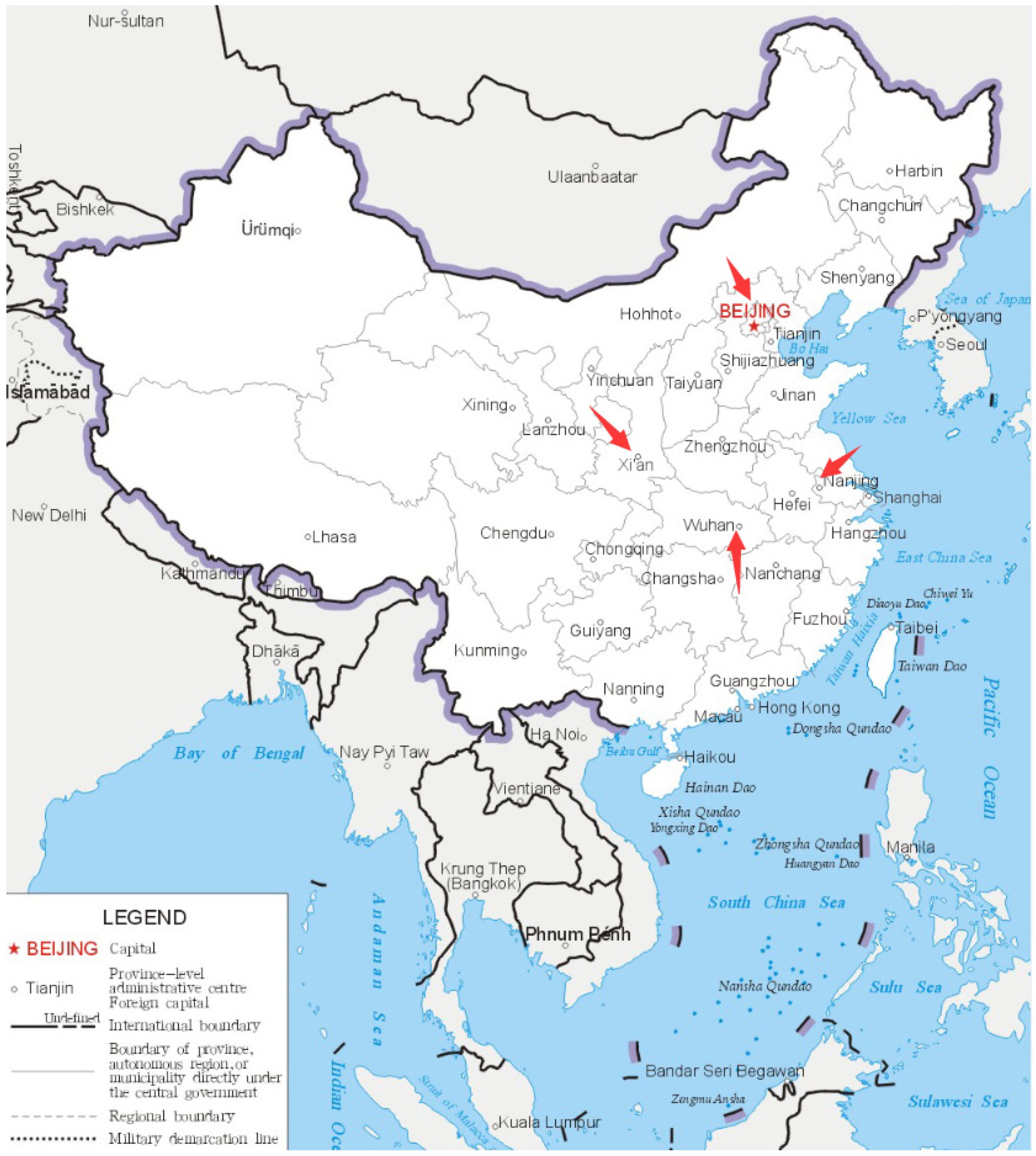
The study areas include some major cities in China. Considering data availability, the rental houses in four cities are included in this study: Wuhan, Nanjing, Beijing, and Xi’an (Figure 1).

• Wuhan is a megacity in Central China. It is an important industrial, science, and education base and a comprehensive transportation center. Wuhan (29°58′–31°22′ N, 113°41′−115°05′ E) has 13 municipal districts with a total area of 8569.15 km², and in 2020, it had a resident population of 12.448 million people.
• Nanjing is an important megacity in Southeast China. It is a science and education base, and a comprehensive transportation center. Nanjing (31°14′−32°37′ N, 118°22′–119°14′ E) has 11 municipal districts with a total area of 6587.02 km², and in 2020, it had a resident population of 9.320 million people.
• Beijing is the capital city of China and the largest city in Northern China. Beijing (39°24′−41°36′ N, 115°42′−117°24′ E) has 16 municipal districts with a total area of 16,410.54 km², and in 2020, it had a resident population of 21.890 million people.
• Xi’an is a megacity in Northwest China. It is an important industrial, science, and education base of China. Xi’an (33°25′−34°27′ N, 107°24′−109.29′ E) has 13 municipal districts with a total area of 10,752 km², and in 2020, it had a resident population of 12.953 million people.

The experiments involving these four different cities are intended to test the availability and generality of our method for different cities. These cities are located in different zones of China (Wuhan: Central China; Nanjing: Southeast China; Beijing: Northern China; Xi’an: Northwest China) and may represent the geographical locational and sociocultural diversity of China as a vast country [44]. There are rising numbers of floating populations in these cities, which means that they have considerable demands for rental housing and flourishing rental housing markets. Thus, we chose them as study areas.

3.2. POI Data

The POI data in this study were captured from the Baidu Map website, which is the largest map service provider in China. The POIs of Baidu Map are classified into 21 primary categories [45], as depicted in

Table 1. The POI data and categories of Baidu Map.

Primary Category	Secondary Category
Food	Chinese restaurants, foreign restaurants, snack shops, cake and dessert shops, coffee shops, tea shops, bars, etc.
Hotel	Star hotels, fast hotels, apartment hotels, etc.
Shopping	Shopping malls, supermarkets, convenience stores, household building materials, digital appliances, shops, markets, etc.
Life and services	Communication business halls, post offices, logistics companies, ticket offices, laundromats, photo shops, real estate intermediaries, public utilities, maintenance points, housekeeping services, funeral services, lottery sales points, pet services, newspaper booths, public toilets, etc.
Beauty	Beauty, hairdressing, manicure, body beautification, etc.
Scenic spot	Parks, zoos, botanical gardens, amusement parks, museums, aquariums, beach baths, cultural relics, churches, scenic spots, etc.
Recreation and entertainment	Holiday villages, farmhouses, cinemas, KTV, theatres, song and dance halls, internet cafes, playgrounds, bath massages, leisure squares, etc.
Sports fitness	Stadiums, extreme sports venues, fitness centers, etc.
Education and training	Colleges and universities, secondary schools, primary schools, kindergartens, adult education, parent–child education, special education schools, scientific research institutions, training institutions, libraries, science and technology museums, etc.
Cultural media	Press and publishing, radio and television, art groups, galleries, exhibitions, cultural palaces, etc.
Medical care	General hospitals, specialized hospitals, clinics, pharmacies, medical institutions, sanatoriums, emergency centers, CDC, etc.
Automobile service	Automobile sales, automobile maintenance, automobile detailing, automobile parts, car rental, automobile testing grounds, etc.
Transport facilities	Railway stations, long-distance bus stations, ports, parking lots, gas stations, service areas, toll stations, bridges, etc.
Finance	Banks, ATMs, credit cooperatives, investment and financing, pawnbrokers, etc.
Real estate	Office buildings, residential areas, dormitories, etc.
Company and business	Companies, parks, agriculture, forestry, horticulture, factories and mines, etc.
Government organization	Governments of all levels, administrative units, public prosecution and law institutions, foreign-related institutions, party groups, welfare institutions, political and educational institutions, etc.
Entrance and exit	Expressway exits, expressway entrances, airport exits, airport entrances, station exits, station entrances, parking lot entrances, bicycle high-speed exits, bicycle high-speed entrances, etc.
Natural feature	Islands, mountains, water systems, etc.
Administrative landmark	Provinces, provincial cities, prefecture-level cities, districts, counties, business districts, towns, villages, etc.
Address	Address points, etc.

. Administrative landmarks and addresses are not considered in our study because they are map features rather than entities. Therefore, 19 primary categories and 134 secondary categories are taken into account. We collected the POIs of Baidu Map in February to March 2020, and finally, more than 1.7 million POI data were obtained for the four cities.

3.3. Rental House Data

The rental house data in the study are from the commonly used real estate website, Lianjia [46]. Recent studies have demonstrated that the data on this website are effective for housing price analysis [47,48]. All of the rental house samples were captured from Lianjia, and data collection occurred between February and July 2020. The attributes of the houses (the rental price, the area, the information of the community, etc.) can be obtained via data collected from the website. Due to the data accessibility, only the whole rental houses were considered in this research. The data were screened for houses with civil electricity and water, and extreme values were excluded. To control the residential density of the houses, for each city, the samples with extremely high plot ratios (of the communities) in the top 5% were eliminated, since residential density is negatively related to rental prices and a dense environment is more likely to result in congestion and the invasion of privacy. Approximately 239,000 rental samples were obtained (Wuhan: 54,466, Nanjing: 32,076, Beijing: 109,683, Xi’an: 43,289). The rental house price is the dependent variable in this paper, and the rental house prices of the samples in this research range from 6.0~148.8 RMB/m²/month (calculated as the unit price). The descriptions of the rental prices and relevant attributes are shown in

Table 2. The description of the rental house price and relevant attributes.

Variable	The Explanation and the Measurement Method for the Variables	Expected Sign	Type
Area	Square meters of the living area (m2)	-	Structural variables
TotalFloor	The total number of floors of the building	Unknown
Level	The level of the floor on which the unit is situated. (1: “low-level”, <1/3 of the total floor value of the building; 2: “middle level”, between 1/3 and 2/3 of the total floor value, 3: “high level”, >1/3 of the total floor value)	Unknown
Age	The age of the building (calculated by subtracting the construction month from the transaction month, and divided by 12 (so it is in years))	-
Age-squared	The squared value of “Age” [49]	+
Month	The (monthly) time trend variable. The earliest rental date in the dataset of this paper is February 2020. Thus, the observation of this sample takes the value of 1 for the “Month” variable; then, it is 2 for the houses rented in March 2020, etc.	Unknown
Spring	A dummy variable for whether the house is rented in the first quarter of the year (1: the transaction date is January, February, or March; 0: otherwise)	Unknown
Summer	A dummy variable for whether the house is rented in the second quarter of the year (1: the transaction date is April, May, or June; 0: otherwise)	Unknown
Autumn	A dummy variable for whether the house is rented in the third quarter of the year (1: the transaction date is July, August, or September; 0: otherwise)	Unknown
Room	The number of bedrooms	+
Hall	The number of halls	-
Toilet	The number of toilets	Unknown
South	Whether the room faces south (1: when the direction description of the house contains “south”; 0: otherwise)	+
North	Whether the room faces north (1: when the direction description of the house contains “north”; 0: otherwise)	+
East	Whether the room faces east (1: when the direction description of the house contains “east”; 0: otherwise)	+
West	Whether the room faces west (1: when the direction description of the house contains “west”; 0: otherwise)	-
PlotRatio	The gross floor area of the building divided by the area of the community.	Unknown
Green	The greening rate of the community	+
ParkSpace	The number of parking spaces of the community	+
Fee	The property management fee of the house (RMB /m2/month)	+
DCBD	The distance to the CBD (km)	-	Locational variables
Dbus	The distance to the nearest bus station (km)	-
Dsub	The distance to the nearest metro station (km)	-
DshopCen	The distance to the nearest shopping center (km)	-
Dpark	The distance to the nearest park (km)	-	Neighborhood variables
DpriSch	The distance to the nearest primary school (km)	-
DsecSch	The distance to the nearest middle school (km)	-
Dnurs	The distance to the nearest nursery school (km)	-
Dhosp	The distance to the nearest hospital (km)	-
Price	The rental price of the house (RMB/m2/month)

, and the statistics of these data are depicted in

Table A1. The statistics of the rental house price data and relevant attributes of the study areas.

Variable	Mean				Std.				Type
	Wuhan	Nanjing	Beijing	Xi’an	Wuhan	Nanjing	Beijing	Xi’an
Area	91.89	66.58	55.04	86.24	33.96	32.16	31.58	42.60	Structural variables
TotalFloor	22.65	16.24	14.70	27.58	11.97	13.56	8.01	7.60
Level	2.11	1.95	1.96	2.00	0.69	0.68	0.77	0.68
Age	11.07	15.03	17.66	8.17	6.18	7.32	9.37	4.16
Age-squared	152.13	279.08	406.07	85.32	161.57	274.56	416.80	88.12
Month	4.14	4.30	4.43	4.16	1.03	1.74	1.65	1.68
Spring	*	*	*	*	*	*	*	*
Summer	*	*	*	*	*	*	*	*
Autumn	*	*	*	*	*	*	*	*
Room	2.22	1.97	2.14	2.00	0.81	0.87	0.90	0.89
Hall	1.60	1.28	1.07	1.43	0.53	0.53	0.44	0.75
Toilet	1.21	1.03	1.14	1.19	0.44	0.37	0.44	0.47
South	*	*	*	*	*	*	*	*
North	*	*	*	*	*	*	*	*
East	*	*	*	*	*	*	*	*
West	*	*	*	*	*	*	*	*
PlotRatio	3.27	1.38	2.23	4.03	1.63	0.98	0.90	1.48
Green	0.33	35.36	31.01	36.40	0.07	9.92	7.09	7.70
ParkSpace	791.32	569.48	618.57	1080.70	1056.91	666.48	2714.80	1400.44
Fee	1.79	0.92	1.06	1.33	0.83	0.69	1.52	0.64
DCBD	7.06	11.33	18.86	17.32	5.98	6.69	12.21	7.96	Locational variables
Dbus	2.09	0.21	0.27	0.25	1.67	0.12	0.14	0.70
Dsub	4.21	1.28	2.37	2.04	3.94	1.29	5.13	2.35
DshopCen	1.43	1.74	3.38	1.29	1.35	1.14	5.89	0.93
Dpark	1.57	1.06	6.38	1.70	1.10	0.68	8.75	1.00	Neighborhood variables
DpriSch	0.88	10.47	2.43	0.83	0.90	5.00	5.23	0.46
DsecSch	1.00	8.41	2.39	1.38	0.85	5.57	4.66	0.81
Dnurs	0.43	4.09	1.63	0.42	0.43	2.88	4.24	0.35
Dhosp	0.28	0.79	2.79	0.53	0.28	0.58	5.53	0.55
Price	33.32	60.03	95.94	29.94	11.24	24.37	44.28	10.25

*: not applicable for dummy variables.

of Appendix A.

In this research, all of the geographic information was transformed into the Baidu metric coordinate system since the POI data of this research are collected from Baidu Map.

4. Method

4.1. Principal Housing Price Models

4.1.1. HPM

The HPM is a principal pricing model and is the basis of other housing price models [6]. It is introduced and considered as a control group in this study. HPM believes that a house or rental house can be considered a commodity and that its price is made up of many different factors. The factors of rental houses are usually considered to follow the factors of the selling houses [10,19], including 3 types: structural variables, locational variables, and neighborhood variables. Based on the previous studies [4,25,47] and the situation of our available data, the factors considered in this research are listed as follows: the structural variables include the area of the house (Area), the number of total floors (TotalFloor), floor level of the house (Level), number of rooms (Room), halls (Hall), toilets (Toilet), plot ratio of the community (PlotRatio), greening rate of the community (Green), number of parking spaces in the community (ParkSpace), the property management fee (Fee), the age of the building (Age) and its squared value (Age-squared) [49], the monthly trend variable (Month), the seasonality dummy variables (Spring, Summer and Autumn), and house orientation dummy variables (South, North, East, West); locational variables include the distance to the CBD (DCBD) and distances to the nearest subway station (Dsub), bus stop (Dbus), and shopping center (DshopCen); neighborhood variables include the distance to the nearest park (Dpark), hospital (Dhosp), middle school (DsecSch), primary school (DpriSch), and nursery (Dnurs). Since studies have shown that the road network distance can provide additional and useful insights into the housing price dataset and improve the accuracy of relevant models [16,50], the distances correlated with POIs in this study are all measured as the road network distance. The definitions, statistical values, and expected effects on rental price are listed in Table 2.

The basic model of the HPM can be Y = f (X, β, ε), where Y is the rental price, X is the characteristic vector consisting of each variable of the house, β is the coefficient in front of each factor, and ε is the residual term. Practically, the model is generally implemented by means of MLR, as follows:

$$y={\beta }_0+{\displaystyle \sum _{j=1}^m{\beta }_j{x}_j+\epsilon }$$

(1)

where β_j represents the MLR parameter for the jth explanatory variable x_j, and m is the number of explanatory variables.

4.1.2. GWR

The HPM is essentially a global ordinary least squares (OLS) model. Although the model can explain the affecting factors, the fitting accuracy is often insufficient. This insufficiency is because a house is not only correlated with the various factors in the HPM, but also closely related to the geographical location: the rental price of a house will be affected by the characteristics and prices of the neighboring houses. The spatial heterogeneity and regional diversity may cause a discrepancy in the parameter β of the factors. Thus, the rental price is more suitable for a local regression model.

Fotheringham introduced the GWR model [5], which is a geographical extension of OLS. The attribute coefficients of GWR can be viewed as a semi-logarithmic function of the change of the explanatory variable [24]. GWR considers geographical heterogeneity and allows the variations of local parameters, which is formulated as:

$$y_i={\beta }_{i0}(u_i,v_i)+{\displaystyle \sum _{k=1}^m{\beta }_k(u_i,v_i)}{x}_{ik}+{\epsilon }_i, i=1,2,\dots n$$

(2)

where $(u_i,v_i)$ represents the coordinates of sample i, ${\beta }_{ik}(u_i,v_i)$ represents the local parameter of the kth variable of the sample i, which varies for different locations, ${\beta }_{i0}(u_i,v_i)$ is the intercept value, and ${\epsilon }_i$ is the error term. The GWR approach is superior for its ability to reveal the spatial heterogeneity. β_k(u_i, v_i) can be estimated as follows:

$$\hat{\beta }(u_i,v_i)={(X^{T}W(u_i,v_i)X)}^{-1}{X}^{T}W(u_i,v_i)Y$$

(3)

where the weighting matrix W is a diagonal matrix and the off-diagonal elements are all zero, W(u_i, v_i) = dia(W_i1, W_i2, …, W_ij, …, W_in). As declared above, the locations of all rental houses have been transformed into the Baidu metric coordinate system. The geographical weight of the sample i and sample j are represented by W_ij. In this study, we obtain the weighting matrix with the fixed Gaussian kernel function:

$$W_{ij}=\exp (-d_{ij}^2/b^2)$$

(4)

where d_ij is the distance between houses i and j, and b is a non-negative parameter (bandwidth) that represents the decay degree with the distance. The bandwidth (b) is a very important parameter, and the appropriate bandwidth can be selected based on the minimum Akaike information criterion (AICc) for the GWR model [51]. For data with some geographical correlations, the fitting accuracy of the GWR model is substantially greater than that of the global regression method (HPM) because spatial heterogeneity and locational discrepancy are taken into account.

4.1.3. FCNN—A Deep Learning Model

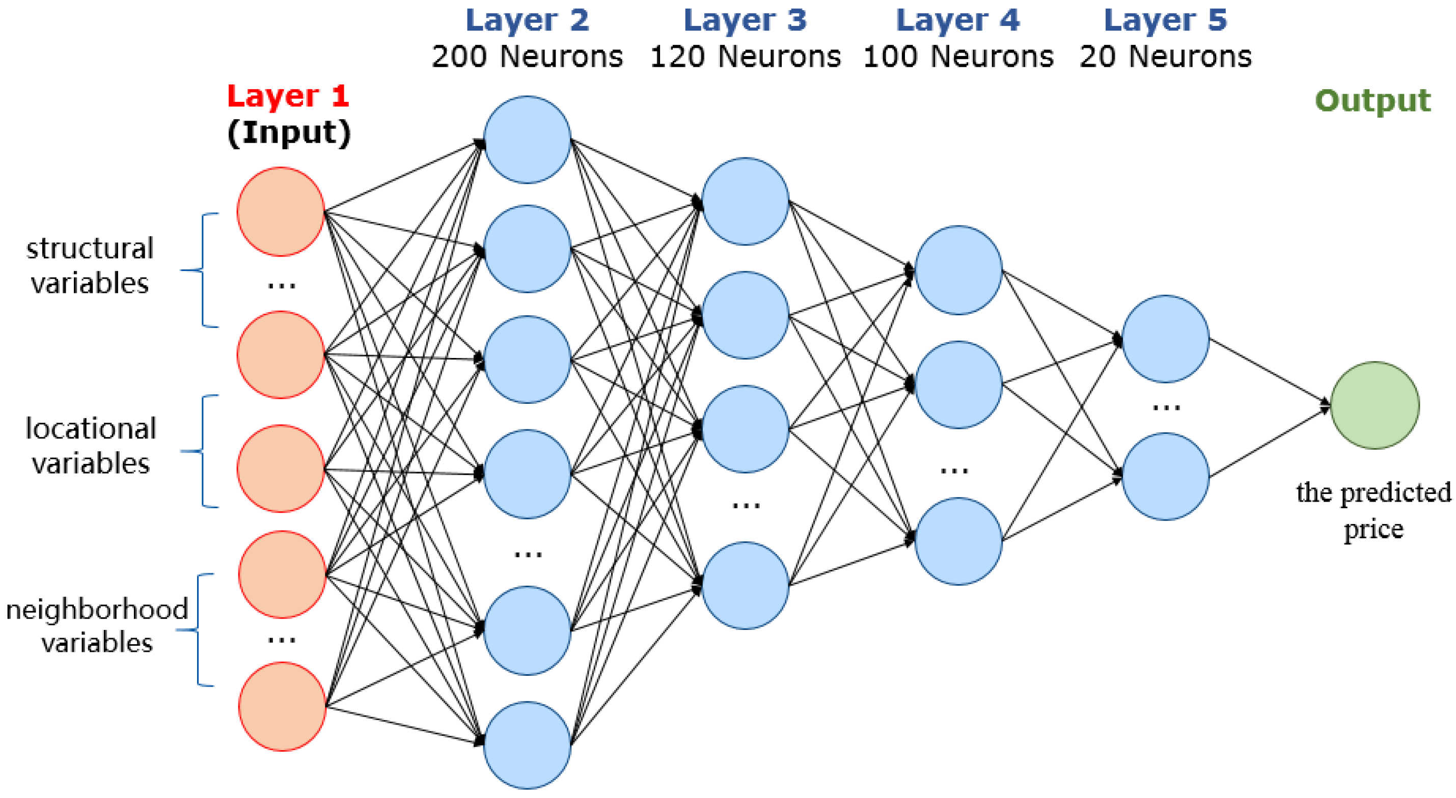
Deep learning commendably supports big data because of its powerful generalization and automation capability and has been widely used in recent years [13]. In this study, we designed a 5-layer fully connected neural network (FCNN) for house rental price and its factors. As shown in Figure 2, the input layer is the vector of the factors, including structural variables, locational variables, and neighborhood variables; there are 4 hidden layers, and the numbers of neurons for them are 200, 120, 100, and 20, respectively; the output layer is the predicted value of the rental house price.

Deep learning can address the nonlinear and complex relationships [3] implied by the variables, which is crucial for the fitting of housing prices. The algorithm of deep learning in this study is: the learning aim is to minimize the sum of the residuals of the predicted and actual values; the activation function is ReLU [52]; the back propagation algorithm is the gradient descent algorithm [53]; for each step, the training number of samples (batch size) is 64; the initial learning rate, the attenuation of learning rate, and the attenuation of the sliding average are set to 0.8, 0.99, 0.99, respectively; the L2 regularization [54] is included in the network for eliminating overfitting. The loss function of the FCNN can be formulated as:

$$\mathrm{loss}={\displaystyle \sum {(Y-Y^{\ast })}^2}+0.0001\ast {\displaystyle \sum _{i=1}^l{w}_i^2}$$

(5)

where $y_i$ represents the predicted value, $y_i^{\ast }$ represents the true value, l is the number of hidden layers, and w_i is the neuron parameters in each hidden layer. For deep-learning methods, all of the data should be divided into 2 parts: the training set and the test set. The training process is carried out in the training set to minimize the value of “loss”. For every sample in deep learning, the values of each variable have been normalized to 0~1 to avoid divergence of the model. After the training is completed, the model is run on the test set to estimate the model’s fitting accuracy and predictive power for unknown samples.

4.2. FCNN–GWR—The Combination of Deep Learning and GWR

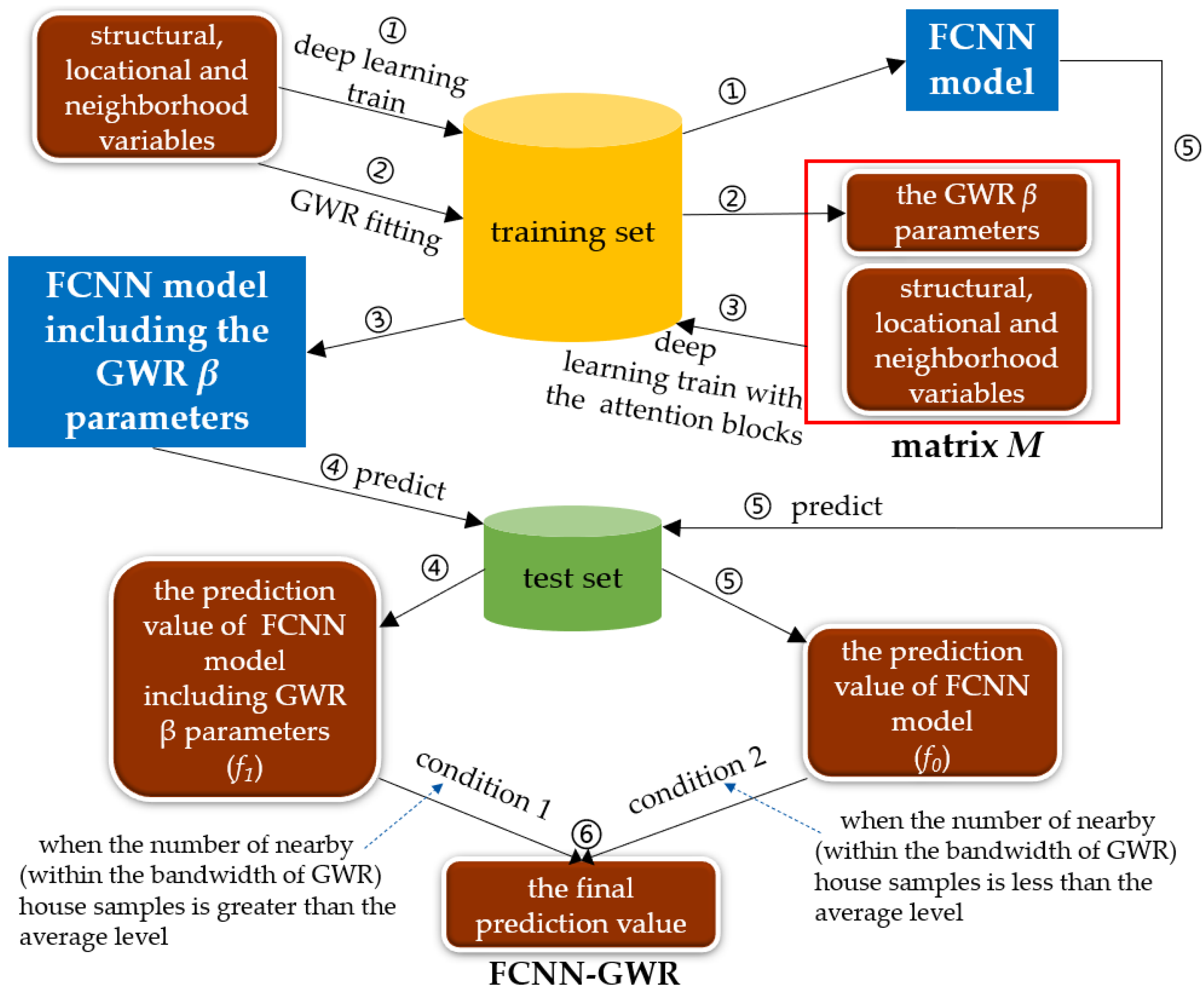
GWR cannot characterize the nonlinear complex characteristics of price, and existing deep-learning methods cannot explicitly process the spatial heterogeneity. Therefore, we propose the FCNN–GWR model, combining deep learning with GWR, which can handle both aspects of the problem. The general idea of the FCNN–GWR model is that the FCNN model can provide an acceptable prediction value for house rental price through deep learning, and the implementation of GWR on this value can optimize it. As the β parameters of GWR contain the spatial heterogeneity and spatial discrepancy of the house rental price, including them in the deep-learning model may explicitly help to optimize the fitting value. We can compose a matrix M, which combines the GWR β parameters with the structural, locational, and neighborhood variables, and then deep learning can be carried out in the matrix M, which may obtain more accurate prediction results. The matrix M = [β₀, β₁, β₂, …, β_m, x₁, x₂, …, x_m], where β₀, β₁, … represents the β parameters in the GWR model as in Equation (2), and x₁, x₂, … means the structural, locational, and neighborhood variables, the same as Equation (1).

As has already been verified, GWR has a clear disadvantage in out-of-sample forecasts, which means that the prediction value of GWR may be not sufficiently reliable when there are not enough samples near the concerning point. Therefore, we only adopt the GWR predictions when there is a relatively large number of samples nearby; when there are fewer samples nearby, just the previous FCNN prediction values are adopted as the final prediction value, which means:

$$y_i=\{\begin{array}{ll}\mathrm{FCNN}({\beta }_0,{\beta }_1,{\beta }_2,\dots ,{\beta }_m,x_1,x_2,\dots ,x_m)& , \mathrm{condition}1\\ \mathrm{FCNN}(x_1,x_1,\dots ,x_m)& , \mathrm{condition}2\end{array}$$

(6)

where for the ith house, y_i denotes its prediction value; other variables are the same as Equations (1) and (2). For a certain house, Condition 1 means that the number of its nearby house samples (within the distance of the bandwidth of GWR) is larger than the average level among all houses ($={{\displaystyle \sum }}_{i=1}^{n}near{s}_i/n$, where $near{s}_i$ represents the number of neighboring samples within the GWR bandwidth for the ith house, and n represents the total number of houses in the dataset); Condition 2 means that the number of nearby (within the distance of bandwidth) houses around it is smaller than the average level among all house samples. Since the bandwidth is a decisive parameter in GWR, and only samples within the distance of the bandwidth of the GWR play a relatively important role in the calculation, we divided the quantities of nearby samples into the 2 conditions by the number of samples within the distance of the bandwidth. When the quantity of nearby samples is smaller than the average, the prediction by GWR may not be sufficiently credible. In these cases, FCNN is more reliable while conversely, weighting geographically may reduce precision. The minus value of accuracy increment of the GWELM in Table 1 of Deng et al. [31] may be attributed to this phenomenon.

Recent studies have proved that the attention mechanism can be effective for the neural networks of the housing price [1,2,9,55]. In our research, the house variables [x₁, x₂, …, x_m] and GWR β parameters [β₀, β₁, β₂, …, β_m] were assigned with an attention block [1] in front of the first fully connected layer, respectively. The attention block can convert the original input characteristics into attended characteristics, in order to identify the important features that influence the rental prices. The attention block can be described as a Softmax-activated fully connected layer, and the algorithm is: $y_k=\Phi \left(h_k\right)x_k=\frac{exp\left(h_k\right)}{{{\displaystyle \sum }}_{k}exp\left(h_k\right)}{x}_k$. where $h_k={\displaystyle \sum }_i{w}_{ki}{x}_i+b_i$, where Φ(·) is the Softmax function, x is the input features, y is the output features, h is the neurons of this fully-connected layer, and w is the weights of the input x. Φ(h) is the soft attention-weighted vector, which can signify the importance of the features of the house variables and GWR β parameters. The variation among attended features y_k would be substantially larger than the variance among the original features x_k as a result of the attention block, suggesting that the important characteristics for the house rental price are emphasized in the network, and it would benefit the convergence and performance of the model.

In the FCNN–GWR model, the data should be divided into the training sets the test sets. The process of FCNN–GWR is shown in Figure 3 and can be described as follows:

Step 1: Train the FCNN model on the training set with the structural, locational, and neighborhood variables of the house.

Step 2: Execute the GWR model on the training set with the structural, locational, and neighborhood variables. Then, the β parameters of GWR can be calculated for each house via GWR fitting.

Step 3: Put the GWR β parameters, and the structural, locational, and neighborhood variables together to make up the matrix M. Through a deep-learning training with the matrix M wrapped with the attention blocks, the FCNN model including the GWR β parameters (and structural, locational, and neighborhood variables) can be obtained.

Step 4: Predict the price value on the test set with the FCNN model including the GWR β parameters (obtained in Step 3). The prediction value is referenced as f₁.

Step 5: Predict the price value on the test set with the ordinary FCNN model (obtained in Step 1, only with the structural, locational, and neighborhood variables, without the GWR β parameters). The prediction value is referenced as f₀.

Step 6: On the test set, the final predicted results of FCNN–GWR are obtained according to equation (6): if there are relatively more samples nearby (Condition 1), the final prediction value would be f₁; if there are relatively fewer samples nearby (Condition 2), the final prediction value would be f₀.

Through this method of synthetic training, the FCNN–GWR model not only has the ability to explain the nonlinear complexity of the price but also addresses the spatial heterogeneity explicitly since the method considers the influence of surrounding rental houses. In this paper, FCNN–GWR and other models were used and compared in the study areas to demonstrate the superiority of the proposed model.

4.3. Quantity-Based Locational and Neighborhood Variables

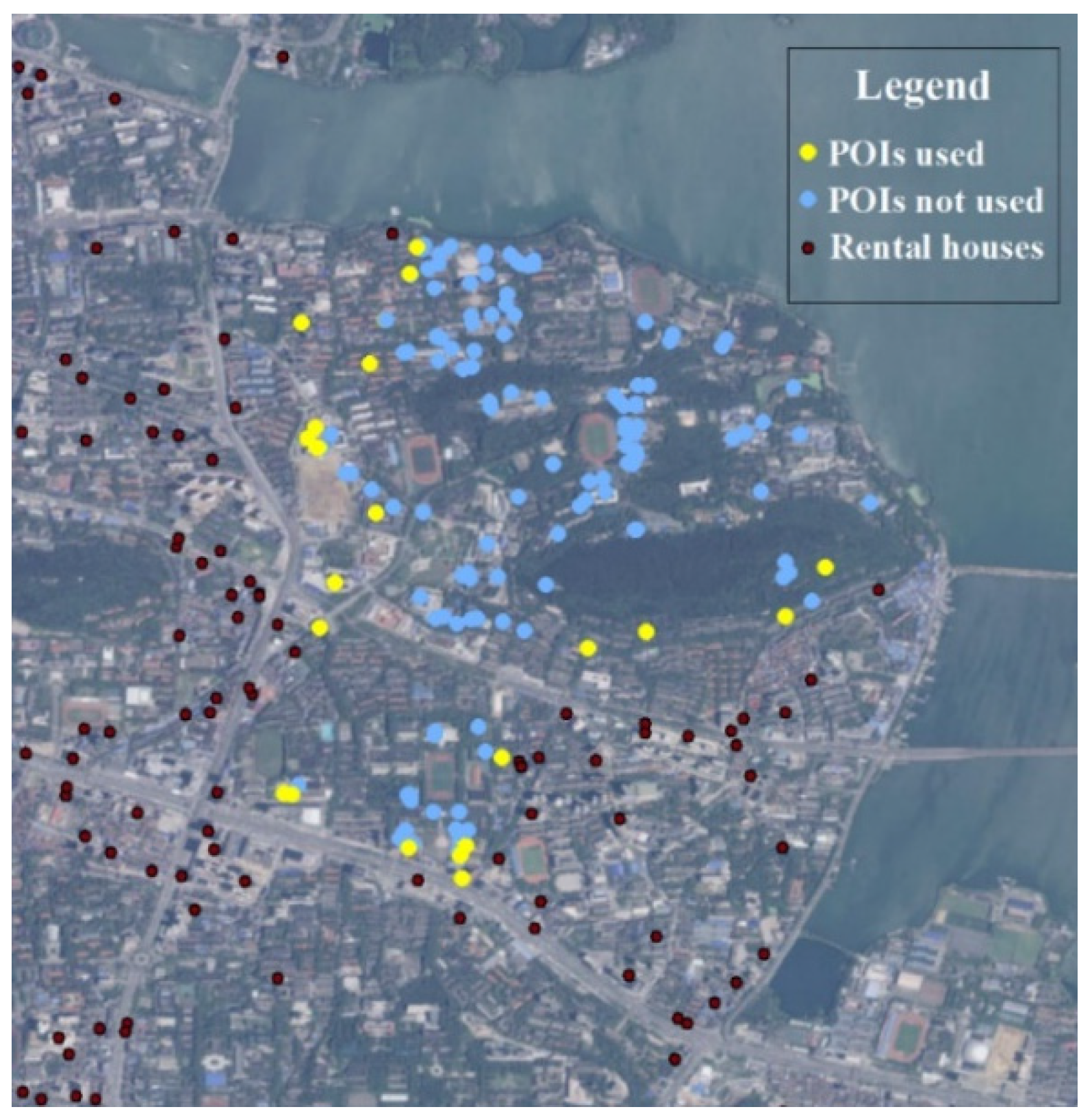
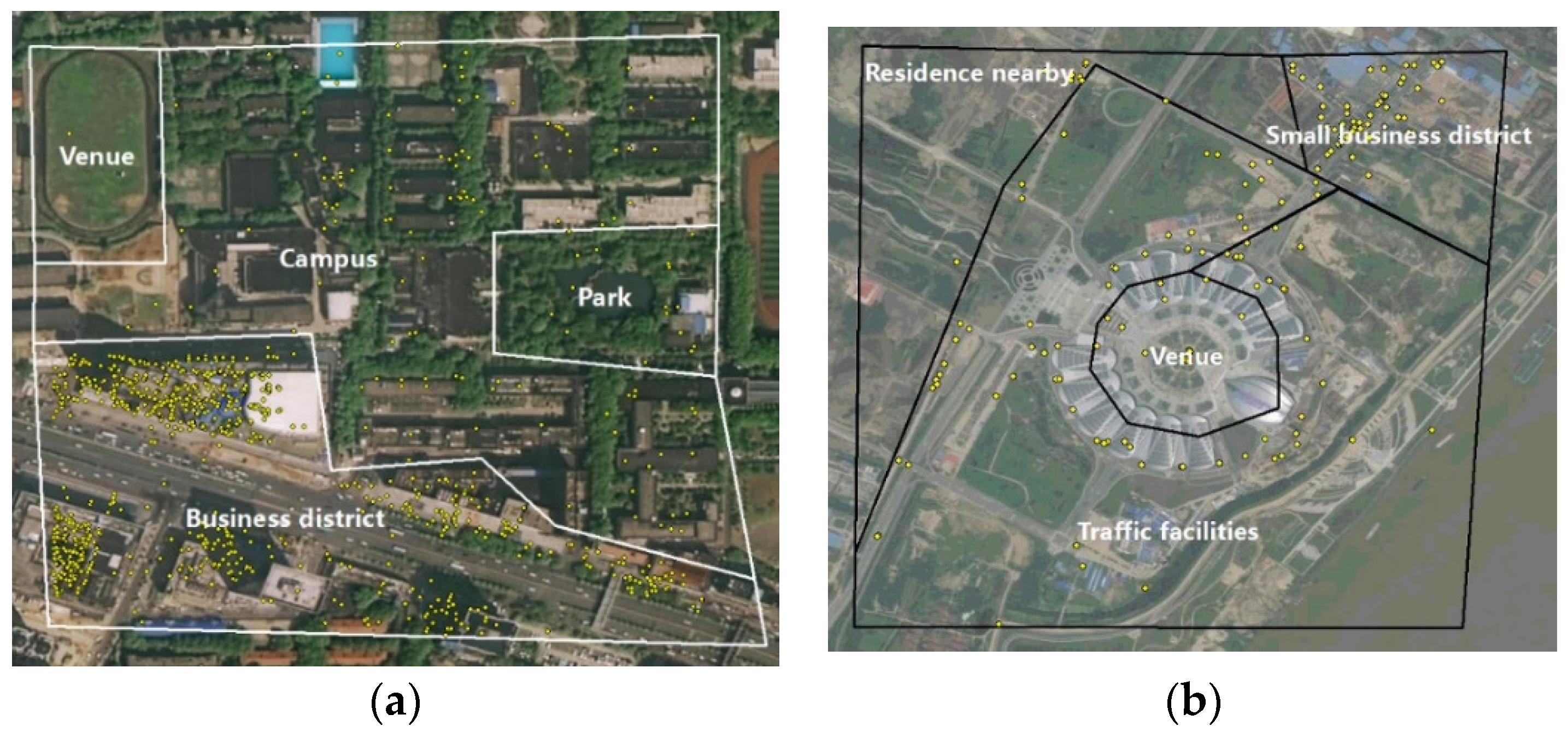
In traditional housing price models, the locational and neighborhood variables include DCBD, Dpark, and so on (Table 2). These factors can reflect the location of the house, but a limited number of variables are allowed in order to avoid the multicollinear problem [56]. In this way, although main factors of the price can be effectively explained, problems still exist. Firstly, these locational and neighborhood variables are distance-based, while expressing the location of houses with the distance may be somewhat inaccurate, which leads to the loss of precision in the house-pricing model. Seo et al. [16], Li et al. [29], and Bency et al. [10] have given the evidence. As shown in Figure 4, there are many POIs typed “school” in this area. When calculating the locational and neighborhood variables of the houses in this area, only the information of the blue points is actually used, which are the “nearest” school POIs to the houses; the information of the neighboring yellow points is not included, just because they are not the “nearest” ones to the houses. In other words, the locational information formed by these yellow points is discarded rather than exploited, which may influence the accuracy of the price model. Secondly, some variables are excluded from the model since they are similar to other variables, the model may lose a certain amount of information. These variables can also contribute to the housing price to a certain extent.

To solve this, we propose another method to measure the locational characteristics of the house: the quantity-based locational and neighborhood variables. In our perspective, the number and the combination of the various kinds of POIs surrounding a house can better reflect its locational characteristics. For example, Figure 5a is the place near a gate of a school, with very dense POIs around it. It is not reasonable to consider only the selected “nearest” POI since other neighboring POIs also contribute to the locational characteristics. To consider the influences of other POIs, a better way is to calculate the number of every type of POI nearby. The number and the combination of every type of POI can better reflect the location characteristics of houses locally. For example, in Figure 5a there are 1301 commercial POIs, 68 traffic POIs, 20 stadium POIs, and 123 school POIs. The number of commercial and school POIs is very large, which implies that this place may be the intersection between the school and the commercial district. For another example, Figure 5b is a newly built venue in Wuhan. There are 104 business POIs, 53 transportation POIs, 6 stadium POIs, and no school POIs nearby. The number of subways, bus, parking, and other transportation facilities is very large, but the number of commercial and school POIs is very small, which demonstrates the characteristics of this place as a new infrastructure and new venue. Therefore, the locational characteristics of a place can be reflected in the form of the above.

The amount of distribution of different types of POIs near a house can be measured to express the quantity characteristics of POIs described above. In fact, the Kernel Density Estimation (KDE) [48] is a practical way to measure the number and density of the points near a certain place, which is a robust analytical tool in GIS for model discovery and spatial statistical and spatiotemporal data mining. In this research, KDE is adopted and the estimated density value of KDE for different types of POIs can be used as “quantity-based variables” for expressing the characteristics of the rental houses, that is:

$$\eta (s_j)={\displaystyle \sum _{k=1}^{N_{\mathrm{j}}}\frac{1}{h^2}}K(\frac{\mathrm{dis}t(s_j,x_{j,k})}{h})$$

(7)

where η(s_j) is the estimated density value of the jth type of POIs for a house sample, N_j is the total number of the jth type of POIs, dist(s_j, x_j,k) is the distance between the location of the house and the location of the kth POI in the jth type of POIs, K(·) is the penalty function (also called kernel function in KDE); and h is the bandwidth of the kernel function, which represents the smoothing effect of the kernel function. If we put [η(s₁), η(s₁), …, η(s_j), …], the estimated density values for all types of POIs, together, they can represent comprehensive locational and neighborhood characteristics for a rental house. The combination of [η(s₁), η(s₁), …, η(s_j), …, η(s_N)] is labeled as “quantity-based locational and neighborhood variables” in this paper.

From the formula above, we learn that the kernel function K(·) and the bandwidth h are 2 parameters that KDE requires. In this research, 4 types of common-used kernel functions are tested to find a suitable kernel and bandwidth for the quantity-based locational and neighborhood variables: the Triangular Kernel, the Gaussian Kernel, and the Laplacian Kernel. We put the structural variables and the “quantity-based locational and neighborhood variables” together, to construct the vector F, which represents the overall factors of the rental house price:

$$F=[s{v}_1,s{v}_2,\dots ,s{v}_Q,\eta (s_1),\eta (s_2),\dots ,\eta (s_N)]$$

(8)

where sv represents a structural variable of the house (in Table 2); Q and N represent the number of the structural variables and locational and neighborhood variables, respectively. The different types of kernel functions and bandwidths would be tested and optimized to find a best one to make the factors F to get a highest R² in the OLS model related to the rental house price.

$$R^2=\frac{n{\displaystyle {\sum }_{i=1}^n{r}_{i,o}{r}_{i,s}-{\displaystyle {\sum }_{i=1}^n{r}_{i,o}{\displaystyle {\sum }_{i=1}^n{r}_{i,s}}}}}{\sqrt{n{\displaystyle {\sum }_{i=1}^n{r}_{i,o}^2}-{({\displaystyle {\sum }_{i=1}^n{r}_{i,o}})}^2}\sqrt{n{\displaystyle {\sum }_{i=1}^n{r}_{i,s}^2}-{({\displaystyle {\sum }_{i=1}^n{r}_{i,s}})}^2}}$$

where r_i;o and r_i;s are the observed (actual) and simulated (calculated by the model) rental prices (unit: RMB/m²/month) for the ith house, and n is the number of rental house samples in each dataset. By testing we find that the Gaussian Kernel performs the best for all the 4 cities and is chosen as the KDE kernel for generating the quantity-based locational and neighborhood variables in this study. After optimizing, the KDE bandwidth h of the 4 cities is determined as 12,657.4 m, 18,495.5 m, 11,549.4 m, 14,386.9 m for Wuhan, Beijing, Nanjing, and Xi’an, respectively.

The quantity-based locational and neighborhood variables are more comprehensive than the traditionally used locational and neighborhood variables in Table 2 and better reflect the multiscale and comprehensive geographical characteristics of the location. To compare with the “quantity-based” variables, the distances to the 134 types of POIs can also be the locational and neighborhood variables, and they are introduced and labeled as “distance-based locational and neighborhood variables” in this paper. Compared with distance-based and quantity-based variables, the “traditional locational and neighborhood variables” refer to the locational and neighborhood variables in Table 2, which includes 9 frequently used variables. It should be noted that the traditional, distance-based and quantity-based locational and neighborhood variables are all correlated with the distance to the POIs. The distances correlated with POIs in this study are measured as the road network distance, which can be measured through GIS network analysis. Then each kind of locational and neighborhood variable can be generated: the traditional variables and distance-based variables are generated by the nearest distance to a certain kind of POI; the quantity-based variables are generated by the KDE kernel functions and bandwidths.

The “distance-based” and “quantity-based” locational and neighborhood variables contain large, complex, similar, and multicollinear factors, which is the situation where deep-learning methods perform well. Hundreds of locational variables provide a sufficient number of vectors for learning and make the models more accurate. However, it should also be noted that the problem of multicollinearity inevitably exists among the very large number. Apparently, if these similar and multicollinear factors are employed in the HPM and GWR model, we cannot evaluate their impacts on the price through the model anymore. The main role of quantity-based variables is to improve the fitting accuracy. That is, the parameter β in the HPM and β(u_i, v_i) in the GWR are no longer of economic significance with the employment of distance-based and quantity-based locational and neighborhood variables, but the fitting accuracy of the model will be greatly improved. Therefore, the meaning of the parameters of the variables (the impact on the price) will not be discussed in this paper. In addition, when calculating β(u_i, v_i) in Equation (3) of the GWR model, the solution of the inverse matrix should be replaced by its pseudoinverse in case there is no inverse matrix.

In this study, traditional locational and neighborhood variables, distance-based locational and neighborhood variables, and quantity-based locational and neighborhood variables will be respectively employed in the HPM, GWR, FCNN, and FCNN–GWR model. When it comes to the distance-based and quantity-based locational and neighborhood variables for each model, the meaning of the parameters in the model will not be discussed as they make no sense, and only the fitting accuracy and predictive ability would be discussed.

4.4. Accuracy Assessment of the Models

The basic rental price models in this study include 4 types: HPM, GWR, FCNN and the proposed FCNN–GWR model. The locational and neighborhood variables of the house include 3 kinds: traditional variables, distance-based variables, and quantity-based variables. For these 4 basic models, all 3 kinds of locational and neighborhood variables will be respectively employed, and the fitting results will be compared. The corresponding experimental groups are labeled as traditional HPM, distance-based HPM, quantity-based HPM, traditional GWR, distance-based GWR, quantity-based GWR, traditional FCNN, distance-based FCNN, quantity-based FCNN, traditional FCNN-GWR, distance-based FCNN-GWR, and quantity-based FCNN-GWR. For the traditional HPM, GWR, FCNN, and FCNN–GWR experiments, the explanatory variables are 20 structural variables and 9 traditional locational and neighborhood variables with no multicollinearity. For the distance-based HPM, GWR, FCNN, and FCNN–GWR experiments, the explanatory variables are the structural variables and 134 distance-based locational and neighborhood variables. For the quantity-based HPM, GWR, FCNN, and FCNN–GWR experiments, the explanatory variables are the structural variables and 134 quantity-based locational and neighborhood variables.

In all of the experiments, the data are divided into a 70% training set and a 30% test set. First, each model would be fitted or trained on the training set; then, the model would be executed on the test set to access the fitting accuracy and predictive power for unknown samples. To enhance the reliability of the experiment, a shuffle and split cross-validation is carried out. The training set and test set are shuffled 4 times, and the results are averaged finally in case that they are determined by inaccurate information.

Several accuracy assessment indicators are calculated to appraise the performance of the above models, referring to existing studies [13,31] and commonly adopted indicators, including the Pearson’s correlation coefficient (Pearson R), the adjusted coefficient of determination (adj R²), the root mean square error (RMSE) and its percentage (%RMSE), and the mean absolute error (MAE) and its percentage (%MAE):

$$\begin{array}{l}\mathrm{Pearson}R=\frac{{\displaystyle {\sum }_{i=1}^n(r_{i,o}-\stackrel{-}{r_o})(r_{i,s}-\stackrel{-}{r_s})}}{\sqrt{{\displaystyle {\sum }_{i=1}^n{(r_{i,o}-\stackrel{-}{r_o})}^2}}\sqrt{{\displaystyle {\sum }_{i=1}^n{(r_{i,s}-\stackrel{-}{r_s})}^2}}}\\ R^2=\frac{n{\displaystyle {\sum }_{i=1}^n{r}_{i,o}{r}_{i,s}-{\displaystyle {\sum }_{i=1}^n{r}_{i,o}{\displaystyle {\sum }_{i=1}^n{r}_{i,s}}}}}{\sqrt{n{\displaystyle {\sum }_{i=1}^n{r}_{i,o}^2}-{({\displaystyle {\sum }_{i=1}^n{r}_{i,o}})}^2}\sqrt{n{\displaystyle {\sum }_{i=1}^n{r}_{i,s}^2}-{({\displaystyle {\sum }_{i=1}^n{r}_{i,s}})}^2}}\\ \mathrm{adj}{R}^2=\frac{(1-R^2)(n-1)}{n-m-1}\\ \mathrm{RMSE}=\sqrt{\frac{{\displaystyle {\sum }_{i=1}^n{(r_{i,o}-r_{i,s})}^2}}{n}}\\ \%\mathrm{RMSE}=\sqrt{\frac{{\displaystyle {\sum }_{i=1}^n{(r_{i,o}-r_{i,s})}^2}}{n}}/\stackrel{-}{r_{\mathrm{o}}}\\ \mathrm{MAE}=\frac{{\displaystyle {\sum }_{i=1}^n|r_{i,o}-r_{i,s}|}}{n}\\ \%\mathrm{MAE}=\frac{{\displaystyle {\sum }_{i=1}^n|r_{i,o}-r_{i,s}|/r_{i,o}}}{n}\end{array}$$

where r_i;o and r_i;s are the observed and simulated rental prices for the ith house (unit: RMB/m²/month), and n is the number of rental houses in each dataset.

5. Results and Discussions

In this section the above-mentioned models will be conducted and analyzed. Since there are many data included in this research, not all of them are able to be displayed in this limited paper. In some cases, the results of Wuhan are preferentially demonstrated as the example, and the data of other cities (Nanjing, Beijing, Xi’an) are employed to strengthen and verify our models and results.

5.1. HPM Results

The HPM model was implemented with MLR, and the result is shown in

Table 3. Accuracy assessment results of HPM with different locational and neighborhood variables—the traditional, distance-based, and quantity-based.

	Wuhan			Nanjing
	Traditional HPM	Distance-Based HPM	Quantity-Based HPM	Traditional HPM	Distance-Based HPM	Quantity-Based HPM
Pearson R	0.7187	0.7857	0.8601	0.6954	0.7505	0.7673
adj R2	0.5197	0.6225	0.7463	0.5088	0.5951	0.6216
RMSE	7.2032	6.3765	5.1945	11.4868	10.8076	10.4635
%RMSE	21.62%	19.17%	15.61%	19.14%	18.04%	17.44%
MAE	5.2871	4.6981	3.5077	8.507	7.8434	7.7032
%MAE	16.70%	13.99%	10.70%	15.45%	14.26%	14.09%
t-test	<0.0001	<0.0001	<0.0001	<0.0001	<0.0001	<0.0001
	Beijing			Xi’an
	Traditional HPM	Distance-Based HPM	Quantity-Based HPM	Traditional HPM	Distance-Based HPM	Quantity-Based HPM
Pearson R	0.7964	0.8266	0.8316	0.5878	0.7494	0.8024
adj R2	0.6633	0.7162	0.7249	0.3423	0.5583	0.6393
RMSE	19.2098	17.9573	17.7323	7.7096	6.4836	6.115
%RMSE	20.01%	18.71%	18.48%	25.73%	21.77%	20.53%
MAE	13.4011	12.2154	11.9717	5.0645	4.3013	4.0390
%MAE	15.78%	14.10%	13.75%	17.57%	14.73%	13.91%
t-test	<0.0001	<0.0001	<0.0001	<0.0001	<0.0001	<0.0001

. For the traditional HPM of the Wuhan dataset, the value of R² is 0.520, suggesting that 52.0% of the variance in the house rental price is explained by this model. The results of other cities are similar. The value of R² is 0.509, 0.663, 0.342 in Nanjing, Beijing, and Xi’an. The HPM can abstract and generalize the factors, and global patterns of the rental prices can be comprehended through it [24,25]. However, the accuracy of the traditional HPM is not high and cannot meet the requirements for estimating and forecasting the price. The results in Table 3 show that the R² values of the distance-based HPM and quantity-based HPM reach 0.623 and 0.746 respectively in Wuhan, which can explain 62.3% and 74.6% of the variance in the rental price. The results of other cities also represent that the distance-based and quantity-based HPM apparently fits better than the traditional HPM. As the quantity-based variables can more comprehensively reflect the characteristics of the house with more geographic objects considered and with a comprehensive geographical perspective, they can greatly increase the accuracy of MLR fitting of its rental price.

5.2. GWR Results

5.2.1. Traditional GWR

The results of GWR on traditional adopted variables are labeled as traditional GWR and are summarized in

Table 4. The results of traditional GWR.

	Wuhan	Nanjing	Beijing	Xi’an
band width	868.5	1042.7	960.2	823.9
adj R2 of traditional GWR (training set)	0.8416	0.6306	0.7665	0.7062
adj R2 of traditional GWR (test set)	0.7558	0.5328	0.7087	0.6148
adj R2 of traditional HPM (test set)	0.5197	0.5088	0.6633	0.3423
AICc of traditional GWR (test set)	8.683 × 10⁴	2.594 × 10⁵	1.140 × 10⁶	1.295 × 10⁵
AICc of traditional HPM (test set)	2.119 × 10⁵	2.940 × 10⁵	1.273 × 10⁶	2.679 × 10⁵

(compared with traditional HPM). In this method the R² values in the test sets are 0.756, 0.533, 0.709, and 0.615 for Wuhan, Nanjing, Beijing, and Xi’an, respectively, which is apparently larger than that of traditional HPM. The AICc values are smaller than that of traditional HPM (All of the values are averaged for the shuffled datasets). It can be seen from the results that traditional GWR has a much higher explanatory ability for the house rental price than traditional HPM. As mentioned before, this is because GWR takes into account the spatial heterogeneity in the rental house prices, which is not a negligible property for rental house price modeling.

5.2.2. Distance-Based GWR and Quantity-Based GWR

In case of multicollinearity, when calculating β(u_i, v_i) in the test set of the distance-based and quantity-based GWR method, the solution of the inverse matrix in Equation (3) should be replaced by the pseudoinverse. Then, GWR prediction would be executed in the test set [57]. With the Wuhan dataset as an example, the performance of each method in the training set and test set can be seen in

Table 5. The performances of GWR and FCNN in the training set and the test set of Wuhan.

Method	Distance-Based GWR			Distance-Based FCNN
	Training Set	Test Set	Difference between Training and Test Sets	Training Set	Test Set	Difference Between Training and Test Sets
Pearson R	0.9237	0.8883	−0.0354	0.9211	0.9141	−0.0070
adj R2	0.9072	0.8047	−0.1025	0.8813	0.8682	−0.0131
RMSE	3.092	4.5450	1.4530	3.3609	3.551	0.1901
%RMSE	9.25%	13.61%	4.35%	10.06%	10.63%	0.57%
MAE	2.2676	2.6683	0.4007	2.3721	2.4827	0.1106
%MAE	6.59%	7.77%	1.18%	6.79%	7.11%	0.32%
Method	Quantity-Based GWR			Quantity-Based FCNN
	Training Set	Test Set	Difference between Training and Test Sets	Training Set	Test Set	Difference between Training and Test Sets
Pearson R	0.9498	0.8882	−0.0616	0.9439	0.9344	−0.0095
adj R2	0.9479	0.8379	−0.1100	0.9104	0.8925	−0.0179
RMSE	2.0271	4.5271	2.500	2.9762	3.2923	0.3161
%RMSE	6.09%	13.56%	7.47%	8.92%	9.86%	0.95%
MAE	1.4830	2.4363	0.9533	1.8410	2.0179	0.1769
%MAE	4.44%	7.30%	2.86%	5.65%	6.19%	0.54%

, which suggests that quantity-based GWR performs better than distance-based GWR. Therefore, the quantity-based locational and neighborhood variables are also effective in the GWR model. All GWR methods are superior to the HPM in accuracy for the consideration of the spatial heterogeneity.

Moreover, from the left part of Table 5 it can be seen that the accuracy of the GWR models is good in the training set but decreases significantly in the test set for each indicator. For example, the value of R² decreased by 0.10 in distance-based GWR and decreased by 0.11 in quantity-based GWR from the training set to the test set. As noted by Cajias et al. [7], the GWR model may have overfitting problems and might have a disadvantage in out-of-sample forecasts. For the possible overfitting defect of the GWR model, we tested the FCNN deep-learning method to improve the predictive power of the house rental price.

5.3. Combining the FCNN and GWR

5.3.1. FCNN Results

Similarly, traditional, distance-based, and quantity-based locational and neighborhood variables are employed in the FCNN model which are labeled as traditional FCNN, distance-based FCNN, and quantity-based FCNN, respectively. Taking Wuhan as an example: the traditional FCNN becomes stable after approximately 50,000 steps of training, the distance-based FCNN tends stable after approximately 300,000 steps, and the quantity-based FCNN method achieves stability approximately about 300,000 steps. The results in

Table A2. Accuracy assessment results of each method.

	Wuhan				Nanjing
	Traditional HPM	Traditional GWR	Traditional FCNN	Traditional FCNN-GWR	Traditional HPM	Traditional GWR	Traditional FCNN	Traditional FCNN-GWR
Pearson R	0.7187	0.7985	0.8831	0.9158	0.6954	0.7348	0.8573	0.8783
adj R2	0.5197	0.7558	0.7901	0.8268	0.5088	0.5328	0.7788	0.8202
RMSE	7.2032	5.5664	4.7929	4.5955	11.4868	11.3654	9.3097	8.8566
%RMSE	21.62%	16.77%	14.40%	13.79%	19.14%	18.91%	15.50%	14.73%
MAE	5.2871	3.0454	3.3635	3.2788	8.507	7.1967	6.4888	6.0519
%MAE	16.70%	9.40%	10.57%	10.35%	15.45%	13.20%	11.68%	10.91%
Pearson R range	0.0035	0.0036	0.0029	0.0025	0.0031	0.0032	0.0041	0.004
R2 range	0.0037	0.0032	0.0035	0.0032	0.0066	0.0053	0.0069	0.0062
Pearson R std.	0.0016	0.0014	0.0015	0.0011	0.0017	0.0015	0.0021	0.002
R2 std.	0.0018	0.0016	0.0019	0.0017	0.004	0.0028	0.0033	0.0031
	distance-based HPM	distance-based GWR	distance-based FCNN	distance-based FCNN-GWR	distance-based HPM	distance-based GWR	distance-based FCNN	distance-based FCNN-GWR
Pearson R	0.7857	0.8883	0.9141	0.9288	0.7505	0.8254	0.8901	0.9153
adj R2	0.6225	0.8047	0.8682	0.8922	0.5951	0.6548	0.8419	0.8641
RMSE	6.3765	4.545	3.551	3.466	10.8076	9.8284	8.4661	8.2322
%RMSE	19.17%	13.61%	10.63%	10.41%	18.04%	16.39%	14.09%	13.70%
MAE	4.6981	2.6683	2.4827	2.2425	7.8434	7.1285	5.6652	5.5031
%MAE	13.99%	7.77%	7.11%	6.97%	14.26%	12.96%	10.35%	10.05%
Pearson R range	0.0042	0.0044	0.0054	0.0055	0.0054	0.004	0.0038	0.0044
R2 range	0.0058	0.0052	0.0061	0.0049	0.0075	0.0051	0.0078	0.0057
Pearson R std.	0.0021	0.002	0.0025	0.0024	0.0023	0.0021	0.0022	0.0015
R2 std.	0.0031	0.003	0.0034	0.003	0.0044	0.002	0.0035	0.0031
	quantity-based HPM	quantity-based GWR	quantity-based FCNN	quantity-based FCNN-GWR	quantity-based HPM	quantity-based GWR	quantity-based FCNN	quantity-based FCNN-GWR
Pearson R	0.8601	0.8882	0.9344	0.9534	0.7673	0.9023	0.8919	0.9209
adj R2	0.7463	0.8379	0.8925	0.9192	0.6216	0.6686	0.8455	0.8715
RMSE	5.1945	4.5271	3.2923	3.2285	10.4635	11.1837	8.4302	8.1608
%RMSE	15.61%	13.56%	9.86%	9.69%	17.44%	18.66%	14.06%	13.56%
MAE	3.5077	2.4363	2.0179	1.9748	7.7032	7.032	5.7471	5.5475
%MAE	10.70%	7.30%	6.19%	6.07%	14.09%	12.75%	10.46%	10.12%
Pearson R range	0.0038	0.0047	0.0033	0.0035	0.0027	0.0029	0.0037	0.0048
R2 range	0.0043	0.0061	0.006	0.004	0.0049	0.003	0.0076	0.0055
Pearson R std.	0.002	0.0019	0.002	0.0015	0.0011	0.0013	0.0019	0.002
R2 std.	0.0028	0.0032	0.0024	0.0024	0.0017	0.0014	0.0036	0.0027
	Beijing				Xi’an
	traditional HPM	traditional GWR	traditional FCNN	traditional FCNN-GWR	traditional HPM	traditional GWR	traditional FCNN	traditional FCNN-GWR
Pearson R	0.7964	0.8172	0.9019	0.9205	0.5878	0.8123	0.7546	0.8253
adj R2	0.6633	0.7087	0.8616	0.8839	0.3423	0.6148	0.5701	0.6798
RMSE	19.2098	17.8532	13.983	13.2301	7.7096	6.3072	6.4261	5.9846
%RMSE	20.01%	18.60%	14.65%	13.81%	25.73%	21.16%	21.61%	20.10%
MAE	13.4011	11.4688	9.2452	8.515	5.0645	3.7569	4.3707	3.8722
%MAE	15.78%	12.74%	10.23%	9.37%	17.57%	12.94%	15.25%	13.27%
Pearson R range	0.0022	0.0029	0.002	0.0021	0.0036	0.0031	0.0026	0.0026
R2 range	0.003	0.0035	0.0074	0.0037	0.0041	0.0088	0.0036	0.0035
Pearson R std.	0.001	0.0012	0.0008	0.001	0.0016	0.0013	0.0011	0.0012
R2 std.	0.0014	0.0018	0.0038	0.0013	0.0015	0.0033	0.0014	0.0016
	distance-based HPM	distance-based GWR	distance-based FCNN	distance-based FCNN-GWR	distance-based HPM	distance-based GWR	distance-based FCNN	distance-based FCNN-GWR
Pearson R	0.8266	0.8541	0.8966	0.9093	0.7494	0.8253	0.874	0.8934
adj R2	0.7162	0.7643	0.8469	0.8673	0.5583	0.6723	0.7631	0.7856
RMSE	17.9573	16.7231	14.2703	13.9321	6.4836	5.9612	5.6395	5.4804
%RMSE	18.71%	17.42%	14.91%	14.51%	21.77%	20.00%	18.78%	18.26%
MAE	12.2154	10.6983	8.8871	8.6769	4.3013	3.7842	3.4775	3.3791
%MAE	14.10%	11.89%	9.66%	9.44%	14.73%	12.89%	11.71%	11.77%
Pearson R range	0.0016	0.0014	0.0027	0.004	0.0042	0.003	0.0067	0.0033
R2 range	0.0031	0.0017	0.0044	0.004	0.005	0.004	0.007	0.0045
Pearson R std.	0.001	0.0005	0.001	0.0015	0.002	0.0017	0.003	0.0015
R2 std.	0.0016	0.0008	0.0025	0.0018	0.0021	0.0025	0.0028	0.0023
	quantity-based HPM	quantity-based GWR	quantity-based FCNN	quantity-based FCNN-GWR	quantity-based HPM	quantity-based GWR	quantity-based FCNN	quantity-based FCNN-GWR
Pearson R	0.8316	0.8624	0.915	0.9251	0.8024	0.8373	0.8872	0.9042
adj R2	0.7249	0.7723	0.8822	0.8981	0.6393	0.6849	0.7818	0.8051
RMSE	17.7323	16.5705	13.1021	12.8735	6.115	5.8374	5.5555	5.3923
%RMSE	18.48%	17.26%	13.67%	13.39%	20.53%	19.59%	18.50%	17.95%
MAE	11.9717	10.5897	8.3726	8.2273	4.039	3.7053	3.3941	3.2896
%MAE	13.75%	11.77%	9.21%	9.05%	13.91%	12.62%	11.42%	11.07%
Pearson R range	0.0016	0.0023	0.0023	0.0042	0.0021	0.0019	0.0028	0.0051
R2 range	0.0025	0.0028	0.0042	0.0057	0.0029	0.0023	0.0067	0.0064
Pearson R std.	0.0008	0.0011	0.0012	0.0018	0.001	0.0011	0.0014	0.0026
R2 std.	0.001	0.0014	0.0018	0.0022	0.0012	0.0013	0.0034	0.0034

(in Appendix A) show that the fitting and prediction accuracy of the quantity-based FCNN is higher than that of the traditional and the distance-based FCNN. Besides, the quantity-based FCNN method is the better one in terms of the accuracy indicators among the above HPM, GWR, and FCNN methods.

5.3.2. Comparison of GWR and FCNN

Overall, the GWR model is a linear-based model that reflects the influence of the neighboring house samples; deep learning involves complex nonlinear characteristics but does not directly handle the influence of the neighboring houses. When there are abundant locational and neighborhood variables, for neighboring houses, their characteristic vectors consisting of the structural, locational and neighborhood variables (the x in Equations (1) and (2)) would be very similar. The similar vectors will greatly contribute to the fitting value of these neighboring houses, which to some extent can be seen as an implicit reflection of the neighboring influences. As a result, the FCNN method generally has better results than GWR, both in terms of the distance-based and quantity-based variables, as shown in Table 5 with the example of Wuhan. Moreover, the FCNN models results in much smaller discrepancies between the training sets and test sets than the GWR models. For example, in Table 5, for the quantity-based GWR the R² differs by 0.11 between the training and test sets, and the RMSE differs by 2.5; while for the quantity-based FCNN, the R² differs by only 0.02, and the RMSE differs by only 0.32 between the training and test sets. Therefore, this study also provides evidence for the possible disadvantage of the GWR model in out-of-sample forecasts, and prediction with the FCNN is more stable and robust than using GWR.

5.3.3. FCNN–GWR Results and Discussion

Although the prediction accuracy of the FCNN is clearly higher than that of GWR, the FCNN model does not explicitly handle the influence of neighboring houses; thus, it can be improved. The FCNN–GWR model is proposed by combining deep learning with GWR, which can not only reflect the nonlinearly complicated characteristics of the rental house prices but also explicitly process spatial heterogeneity.

The FCNN–GWR results are shown in Table A2 (in Appendix A) and can be compared with those of the FCNN model and the GWR model. In addition to the indicators introduced in Section 4.4, four indicators are adopted to evaluate the stability of different shuffles of training sets and test sets. They are as follows: (1). Pearson R range: the maximum deviation of the Pearson R values in different shuffles of datasets; (2) R² range: the maximum deviation of the R² values in different shuffles of datasets; (3) Pearson R std.: the adjusted deviation of the Pearson R in different shuffles of datasets; and (4) R² std.: the adjusted deviation of R² in different shuffles of datasets. Finally, the stability of the partition of the training sets is discussed.

When viewed horizontally, Table A2 shows that for each city, quantity-based FCNN-GWR is clearly the best method for predicting rental house prices: all the 6 accuracy indicators obtained the best values among all of the experiments. For models with traditional, distance-based, and quantity-based locational and neighborhood variables, the fitting accuracy of the HPM methods are relatively low. The GWR methods have higher fitting precisions, but the stability and robustness are not very good. The FCNN methods have higher accuracy than GWR, and FCNN–GWR has the highest accuracy. FCNN–GWR includes both the complex nonlinear characteristics and the spatial heterogeneity of the rental house prices and reduces the instability of GWR in areas with relatively sparse samples via Equation (6). Therefore, it has fine precision and stability for the fitting and forecasting of rental house price.

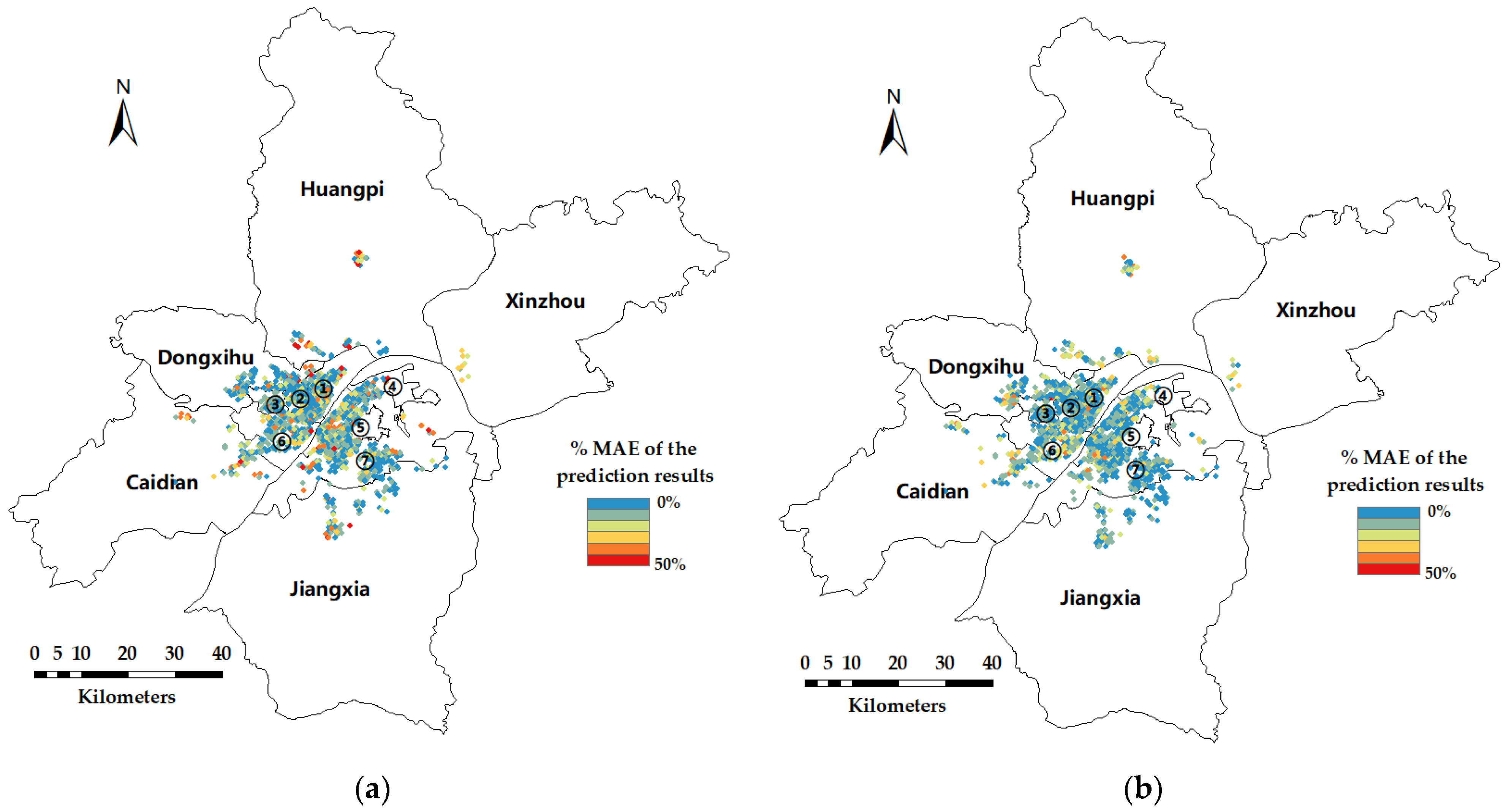
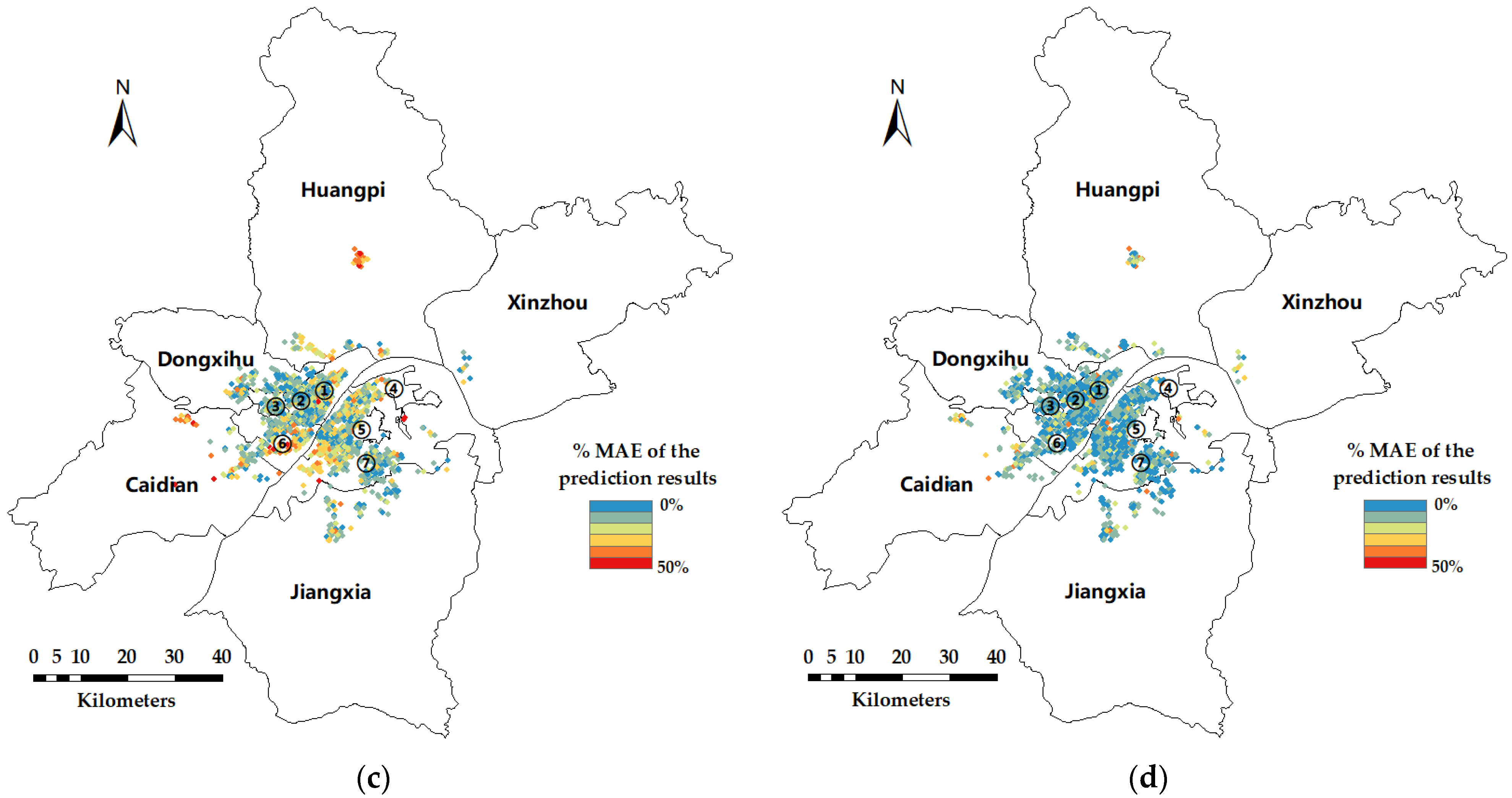
For the four HPM, GWR, FCNN, and FCNN–GWR models, with the quantity-based locational and neighborhood variables, we counted the percentage of the mean absolute prediction error (namely, the %MAE in Section 4.4) of each method for the communities in the Wuhan dataset, and the errors (averaged by all experiments) is visualized in Figure 6. Cold colors (blue and green) mean the average prediction accuracies of these communities are relatively high, and warm colors (red and yellow) mean the prediction accuracies are relatively low. As shown in the figure, the accuracy of the HPM is relatively low (Figure 6c). For GWR, the number of warm-colored dots (Figure 6a) is greater than that for the FCNN (Figure 6b); and for GWR, most of the red dots are located in places where the nearby neighborhoods are relatively sparse, which means there are relatively few samples of houses nearby. This phenomenon suggests GWR is possibly to perform fluctuated in the area where the dots are sparse, or near the margin of the gathered dots. Therefore, it can be inferred that the reliability of GWR prediction may be insufficient when the number of nearby samples around the prediction point is small. When there are many samples nearby (inside the gathered dots), both GWR and FCNN have relatively good performance of accuracy, since GWR and FCNN consider the spatial heterogeneity aspect and the nonlinearity aspect of rental house prices, respectively. FCNN–GWR combines the FCNN and GWR, and it takes into account the nonlinearity and spatial heterogeneity when there are many samples nearby; additionally, only the FCNN is adopted when there are relatively few nearby samples, to avoid the possible instability of GWR in these cases. Therefore, FCNN–GWR can better predict rental house prices.

When Table A2 is viewed vertically, the traditional, distance-based, and quantity-based locational and neighborhood variables can be compared. According to the results, the quantity-based variables perform better than the traditional and distance-based variables under all of the HPM, GWR, FCNN, and FCNN–GWR methods. Therefore, it can be verified that the quantity-based locational and neighborhood variables can take into account more geographic information from a comprehensive perspective, thus supporting the rental price model in obtaining better predictive power compared to the traditional and the distance-based locational and neighborhood variables.

Regarding the stability of different partitions of training sets, in almost all cases, the ranges of R² and Pearson R for different partitions of the datasets are less than 0.008, and the adjusted deviations of R² and Pearson R are less than 0.004, which all remain at not high levels. The result shows that there is no apparent discrepancy under different partitions of training sets, and different shuffles do not apparently affect the precision and generalization ability of our model.

Additionally, the FCNN–GWR proposed in this paper is compared with other previously published models in the Wuhan dataset, including a model of CNN [14], Bin [9] and GWELM [31]. (We do not consider the image part of these models since there are no image data in this study.) Quantity-based locational and neighborhood variables are adopted for these models, and the results are shown in

Table 6. Comparison of FCNN–GWR with some previously published models (in Wuhan).

	FCNN–GWR	CNN [14]	Bin [9]	GWELM [31]
Pearson R	0.9534	0.9285	0.9364	0.9214
adj R2	0.9192	0.8823	0.8902	0.8549
RMSE	3.2285	3.3678	3.3261	3.7874
%RMSE	9.69%	10.11%	9.96%	11.34%
MAE	1.9748	2.0599	2.0387	2.2237
%MAE	6.07%	6.21%	6.12%	6.66%

. Among the methods above, FCNN–GWR performs the best in the indicators of the estimation or prediction of rental house prices. The CNN model of Yu [14] treats housing price variables as an image and can extract the complexity of the relationships among the variables. However, the model does not consider spatial heterogeneity, which is a significant and non-negligible factor, and result in limited performance in estimating rental house prices. It is also questionable whether the pooling layers of the CNN are necessary for the regression of rental house prices. Regarding Bin’s approach [9], although the boosted regression trees in the model can improve the accuracy of the prediction efficiently, the spatial heterogeneity is also absent in the architecture of the model. Thus, the accuracy of the model still has room for improvement. The GWELM proposed by Deng [31] incorporates GWR and ELM, and on principle, it might be able to reveal both the spatial heterogeneity and nonlinear characteristics in rental house prices. However, as discussed above, when the quantity of nearby samples is small, the prediction by the GWR-like method may not be sufficiently dependable. GWELM would have unstable depressing accuracies in such cases and consequently reduce the final accuracy of rental house pricing estimation.

In summary, for the combination of spatial heterogeneity, nonlinear model, and geographical scaling, the proposed quantity-based FCNN–GWR can steadily improve the performance of rental house price modeling. However, at present, the locational and neighborhood variables of this study were derived only from POI data. This model may lose some precision in some cases with complex characteristics, since other multitype data, such as remote sensing images [2], street view images [58], or landscape amenities [59] are not considered. In the future, experiments involving neural networks with the above multitype data will be conducted to further improve the accuracy of the rental house price model. Simplification for the procedure of the model and verification of the models in other cities can also be worthwhile work in the future.

6. Conclusions

In this research, we make efforts to improve the accuracy of the rental house-pricing model. Taking four cities in China (Wuhan, Nanjing, Beijing, and Xi’an) as study areas, we combine deep learning and GWR to grasp both the nonlinear characteristics and spatial heterogeneity and propose the FCNN–GWR model to evaluate rental house prices. In this paper, the results of the HPM, GWR, the FCNN, and the proposed FCNN–GWR are compared in terms of accuracy. The results show that the quantity-based FCNN–GWR model has the highest accuracy. Compared with GWR, the proposed model shows the ability to include the nonlinear complexity of rental house prices, and it presents stable and more-accurate forecasts. Compared with the FCNN deep-learning method, the proposed model explicitly addresses spatial heterogeneity because it considers nearby influences. The work performed in this research verifies that deep learning and GWR explain rental house prices from different perspectives, and the combination of both can improve the evaluation accuracy of rental prices. Moreover, the method proposed in this paper may provide a useful reference for individuals and businesses in their transactions related to rental houses and assist the government in making appropriate policies for the price levels and positions of public rental housing.

The quantity-based locational and neighborhood variables proposed in this paper offer a more comprehensive geographical perspective of locational and neighborhood characteristics. They can express the locational information of houses from a perspective involving more types (134 types of POIs in this study), and more comprehensively (the KDE method used in this study), with more geographic objects taken into account. Our experiments show that quantity-based variables better reflect the location of a rental house compared to the traditionally used and distance-based locational and neighborhood variables, and they help improve the accuracy of the pricing model.

However, the locational and neighborhood variables in this paper were derived only from POI data, which is a limitation of this study. This model may lose some accuracy in some cases with complex characteristics, which might be involved in remote sensing images, street view images, or texts. In the future, experiments involving neural networks with such multitype data will be conducted to further increase the accuracy of rental house price estimation. In addition, there are many parameters and procedures in the architecture of the proposed FCNN–GWR. More kinds of neural networks can be tested to reduce the complexity of the procedures of this work and to improve the performance of the deep-learning model of rental house prices.

References

- Bin, J.; Gardiner, B.; Liu, Z.; Li, E. Attention-Based Multi-Modal Fusion for Improved Real Estate Appraisal: A Case Study in Los Angeles. Multimed. Tools Appl. 2019, 78, 31163–31184. [Google Scholar] [CrossRef]
- Wang, P.-Y.; Chen, C.-T.; Su, J.-W.; Wang, T.-Y.; Huang, S.-H. Deep Learning Model for House Price Prediction Using Heterogeneous Data Analysis Along with Joint Self-Attention Mechanism. IEEE Access 2021, 9, 55244–55259. [Google Scholar] [CrossRef]
- Shimizu, C.; Karato, K.; Nishimura, K. Nonlinearity of Housing Price Structure: Assessment of Three Approaches to Nonlinearity in the Previously Owned Condominium Market of Tokyo. Int. J. Hous. Mark. Anal. 2014, 7, 459–488. [Google Scholar] [CrossRef]
- Liang, X.; Liu, Y.; Qiu, T.; Jing, Y.; Fang, F. The Effects of Locational Factors on the Housing Prices of Residential Communities: The Case of Ningbo, China. Habitat Int. 2018, 81, 1–11. [Google Scholar] [CrossRef]
- Fotheringham, A.S.; Charlton, M.E.; Brunsdon, C. Geographically Weighted Regression: A Natural Evolution of the Expansion Method for Spatial Data Analysis. Environ. Plan. A 1998, 30, 1905–1927. [Google Scholar] [CrossRef]
- Wu, C.; Ye, X.; Ren, F.; Wan, Y.; Ning, P.; Du, Q. Spatial and Social Media Data Analytics of Housing Prices in Shenzhen, China. PLoS ONE 2016, 11, e0164553. [Google Scholar] [CrossRef]
- Cajias, M.; Ertl, S. Spatial Effects and Non-Linearity in Hedonic Modeling Will Large Data Sets Change Our Assumptions? J. Prop. Invest. Financ. 2018, 36, 32–49. [Google Scholar] [CrossRef]
- Bellotti, A. Reliable Region Predictions for Automated Valuation Models. Ann. Math. Artif. Intell. 2017, 81, 71–84. [Google Scholar] [CrossRef] [Green Version]
- Bin, J.; Gardiner, B.; Li, E.; Liu, Z. Multi-Source Urban Data Fusion for Property Value Assessment: A Case Study in Philadelphia. Neurocomputing 2020, 404, 70–83. [Google Scholar] [CrossRef]
- Bency, A.J.; Rallapalli, S.; Ganti, R.K.; Srivatsa, M.; Manjunath, B.S. Beyond Spatial Auto-Regressive Models: Predicting Housing Prices with Satellite Imagery. In Proceedings of the 2017 IEEE Winter Conference on Applications of Computer Vision (Wacv 2017), Santa Rosa, CA, USA, 24–31 March 2017; pp. 320–329. [Google Scholar]
- Jiang, Z.; Shen, G. Prediction of House Price Based on the Back Propagation Neural Network in the Keras Deep Learning Framework. In Proceedings of the 2019 6th International Conference on Systems and Informatics (ICSAI), Shanghai, China, 8–10 November 2019; pp. 1408–1412. [Google Scholar]
- Xu, J. A Novel Deep Neural Network Based Method for House Price Prediction. In Proceedings of the 2021 International Conference of Social Computing and Digital Economy (ICSCDE), Chongqing, China, 28–29 August 2021; pp. 12–16. [Google Scholar]
- Yao, Y.; Zhang, J.; Hong, Y.; Liang, H.; He, J. Mapping Fine-Scale Urban Housing Prices by Fusing Remotely Sensed Imagery and Social Media Data. Trans. GIS 2018, 22, 561–581. [Google Scholar] [CrossRef]
- Yu, L.; Jiao, C.; Xin, H.; Wang, Y.; Wang, K. Prediction on Housing Price Based on Deep Learning. Int. J. Comput. Inf. Eng. 2018, 12, 90–99. [Google Scholar]
- Andrew, M.; Haurin, D.; Munasib, A. Explaining the Route to Owner-Occupation: A Transatlantic Comparison. J. Hous. Econ. 2006, 15, 189–216. [Google Scholar] [CrossRef]
- Seo, K.; Golub, A.; Kuby, M. Combined Impacts of Highways and Light Rail Transit on Residential Property Values: A Spatial Hedonic Price Model for Phoenix, Arizona. J. Transp. Geogr. 2014, 41, 53–62. [Google Scholar] [CrossRef]
- Dong, H. The Impact of Income Inequality on Rental Affordability: An Empirical Study in Large American Metropolitan Areas. Urban Stud. 2018, 55, 2106–2122. [Google Scholar] [CrossRef]
- Won, J.; Lee, J.-S. Investigating How the Rents of Small Urban Houses Are Determined: Using Spatial Hedonic Modeling for Urban Residential Housing in Seoul. Sustainability 2018, 10, 31. [Google Scholar] [CrossRef] [Green Version]
- Liebelt, V.; Bartke, S.; Schwarz, N. Hedonic Pricing Analysis of the Influence of Urban Green Spaces onto Residential Prices: The Case of Leipzig, Germany. Eur. Plan. Stud. 2018, 26, 133–157. [Google Scholar] [CrossRef]
- Yu, T.; Song, Y. Solving the Problem of ‘Cold Weather’ of Public Rental Houses—Based on the Analysis of Government’s Purchase of Public Service. China Econ. Trade Guide (Middle) 2018, 35, 74–76. [Google Scholar]
- Henderson, J.V.; Ioannides, Y.M. A Model of Housing Tenure Choice. Am. Econ. Rev. 1983, 73, 98–113. [Google Scholar]
- Ioannides, Y.M.; Rosenthal, S.S. Estimating the Consumption and Investment Demands for Housing and Their Effect on Housing Tenure Status. Rev. Econ. Stat. 1994, 76, 127–141. [Google Scholar] [CrossRef]
- Rosen, S. Hedonic Prices and Implicit Markets-Product Differentiation in Pure Competition. J. Political Econ. 1974, 82, 34–55. [Google Scholar] [CrossRef]
- Malpezzi, S. Hedonic Pricing Models: A Selective and Applied Review. Hous. Econ. Public Policy 2002, 1, 67–89. [Google Scholar]
- Wu, J.; Wang, M.; Li, W.; Peng, J.; Huang, L. Impact of Urban Green Space on Residential Housing Prices: Case Study in Shenzhen. J. Urban Plan. Dev. 2015, 141, 05014023. [Google Scholar] [CrossRef]
- Anselin, L.; Bera, A.K. Spatial Dependence in Linear Regression Models with an Introduction to Spatial Econometrics. Stat.: Textb. Monogr 1998, 155, 237–289. [Google Scholar]
- Anselin, L. Exploring Spatial Data with Geodatm: A Workbook; Center for Spatially Integrated Social Science: Urbana, IL, USA, 2004; Volume 51, pp. 213–223. [Google Scholar]
- Hastie, T.J.; Tibshirani, R.J. Generalized Additive Models. Stat. Sci. 1986, 1, 297–310. [Google Scholar] [CrossRef]
- Li, S.; Ye, X.; Lee, J.; Gong, J.; Qin, C. Spatiotemporal Analysis of Housing Prices in China: A Big Data Perspective. Appl. Spat. Anal. Policy 2017, 10, 421–433. [Google Scholar] [CrossRef]
- Huang, B.; Wu, B.; Barry, M. Geographically and Temporally Weighted Regression for Modeling Spatio-Temporal Variation in House Prices. Int. J. Geogr. Inf. Sci. 2010, 24, 383–401. [Google Scholar] [CrossRef]
- Deng, M.; Yang, W.; Liu, Q. Geographically Weighted Extreme Learning Machine: A Method for Space-Time Prediction. Geogr. Anal. 2017, 49, 433–450. [Google Scholar] [CrossRef]
- Wang, J.J.; Hu, S.G.; Zhan, X.T.; Luo, Q.; Yu, Q.; Liu, Z.; Chen, T.P.; Yin, Y.; Hosaka, S.; Liu, Y. Predicting House Price with a Memristor-Based Artificial Neural Network. IEEE Access 2018, 6, 16523–16528. [Google Scholar] [CrossRef]
- Fan, G.Z.; Pu, M.; Deng, X.; Ong, S.E. Optimal Portfolio Choices and the Determination of Housing Rents under Housing Market Uncertainty. J. Hous. Econ. 2018, 41, 200–217. [Google Scholar] [CrossRef]
- Yoo, S.; Im, J.; Wagner, J.E. Variable Selection for Hedonic Model Using Machine Learning Approaches: A Case Study in Onondaga County, NY. Landsc. Urban Plan. 2012, 107, 293–306. [Google Scholar] [CrossRef]
- Hu, L.; He, S.; Han, Z.; Xiao, H.; Su, S.; Weng, M.; Cai, Z. Monitoring Housing Rental Prices Based on Social Media: An Integrated Approach of Machine-Learning Algorithms and Hedonic Modeling to Inform Equitable Housing Policies. Land Use Policy 2019, 82, 657–673. [Google Scholar] [CrossRef]
- Rico-Juan, J.R.; de La Paz, P.T. Machine Learning with Explainability or Spatial Hedonics Tools? An Analysis of the Asking Prices in the Housing Market in Alicante, Spain. Expert Syst. Appl. 2021, 171, 114590. [Google Scholar] [CrossRef]
- Roth, A.E. The Shapley Value: Essays in Honor of Lloyd S. Shapley; Cambridge University Press: Cambridge, NY, USA, 1988. [Google Scholar]
- Fu, X.; Jia, T.; Zhang, X.; Li, S.; Zhang, Y. Do Street-Level Scene Perceptions Affect Housing Prices in Chinese Megacities? An Analysis Using Open Access Datasets and Deep Learning. PLoS ONE 2019, 14, e0217505. [Google Scholar] [CrossRef] [PubMed]
- Zhao, Y.; Chetty, G.; Tran, D. Deep Learning with Xgboost for Real Estate Appraisal. In Proceedings of the 2019 IEEE Symposium Series on Computational Intelligence (SSCI), Xiamen, China, 6–9 December 2019. [Google Scholar]
- Hagenauer, J.; Helbich, M. A Geographically Weighted Artificial Neural Network. Int. J. Geogr. Inf. Sci. 2021, 35, 1–21. [Google Scholar] [CrossRef]
- Steentoft, A.A.; Poorthuis, A.; Lee, B.S.; Schlapfer, M. The Canary in the City: Indicator Groups as Predictors of Local Rent Increases. EPJ Data Sci. 2018, 7, 1–15. [Google Scholar] [CrossRef] [Green Version]
- Huang, D.J.; Leung, C.K.Y.; Tse, C.Y. What Accounts for the Differences in Rent-Price Ratio and Turnover Rate? A Search-and-Matching Approach. J. Real Estate Financ. Econ. 2018, 57, 431–475. [Google Scholar] [CrossRef]
- Ullah, F.; Sepasgozar, S.M.E. Key Factors Influencing Purchase or Rent Decisions in Smart Real Estate Investments: A System Dynamics Approach Using Online Forum Thread Data. Sustainability 2020, 12, 4382. [Google Scholar] [CrossRef]
- Su, S.; Zhang, J.; He, S.; Zhang, H.; Hu, L.; Kang, M. Unraveling the Impact of Tod on Housing Rental Prices and Implications on Spatial Planning: A Comparative Analysis of Five Chinese Megacities. Habitat Int. 2021, 107, 102309. [Google Scholar] [CrossRef]
- Baidu. Baidu Map Open Platform. Available online: https://lbsyun.baidu.com/index.php?title=lbscloud/poitags (accessed on 20 November 2021).
- Lianjia. Lianjia Flagship Website. Available online: https://wh.lianjia.com/ (accessed on 20 November 2021).
- Wu, H.; Jiao, H.; Yu, Y.; Li, Z.; Peng, Z.; Liu, L.; Zeng, Z. Influence Factors and Regression Model of Urban Housing Prices Based on Internet Open Access Data. Sustainability 2018, 10, 1676. [Google Scholar] [CrossRef] [Green Version]
- Li, H.; Wei, Y.D.; Wu, Y.; Tian, G. Analyzing Housing Prices in Shanghai with Open Data: Amenity, Accessibility and Urban Structure. Cities 2019, 91, 165–179. [Google Scholar] [CrossRef]
- Bokhari, S.; Geltner, D. Characteristics of Depreciation in Commercial and Multifamily Property: An Investment Perspective. Real Estate Econ. 2018, 46, 745–782. [Google Scholar] [CrossRef] [Green Version]
- Lu, B.; Charlton, M.; Harris, P.; Fotheringham, A.S. Geographically Weighted Regression with a Non-Euclidean Distance Metric: A Case Study Using Hedonic House Price Data. Int. J. Geogr. Inf. Sci. 2014, 28, 660–681. [Google Scholar] [CrossRef]
- Hurvich, C.M.; Simonoff, J.S.; Tsai, C.L. Smoothing Parameter Selection in Nonparametric Regression Using an Improved Akaike Information Criterion. J. R. Stat. Soc. Ser. B-Stat. Methodol. 1998, 60, 271–293. [Google Scholar] [CrossRef]
- Hahnloser, R.H.R.; Sarpeshkar, R.; Mahowald, M.A.; Douglas, R.J.; Seung, H.S. Digital Selection and Analogue Amplification Coexist in a Cortex-Inspired Silicon Circuit. Nature 2000, 405, 947–951. [Google Scholar] [CrossRef]
- Barzilai, J.; Borwein, J.M. Two-Point Step Size Gradient Methods. IMA J. Numer. Anal. 1988, 8, 141–148. [Google Scholar] [CrossRef]
- Schmidhuber, J. Deep Learning in Neural Networks: An Overview. Neural Netw. 2015, 61, 85–117. [Google Scholar] [CrossRef] [PubMed] [Green Version]
- Vaswani, A.; Shazeer, N.; Parmar, N.; Uszkoreit, J.; Jones, L.; Gomez, A.N.; Kaiser, Ł.; Polosukhin, I. Attention Is All You Need. In Proceedings of the Advances in Neural Information Processing Systems, Long Beach, CA, USA, 4–9 December 2017; pp. 5998–6008. [Google Scholar]
- Farrar, D.E.; Glauber, R.R. Multicollinearity in Regression Analysis: The Problem Revisited. Rev. Econ. Stat. 1967, 49, 92–107. [Google Scholar] [CrossRef]
- Harris, P.; Fotheringham, A.S.; Crespo, R.; Charlton, M. The Use of Geographically Weighted Regression for Spatial Prediction: An Evaluation of Models Using Simulated Data Sets. Math. Geosci. 2010, 42, 657–680. [Google Scholar] [CrossRef]
- Li, S.; Jiang, Y.; Ke, S.; Nie, K.; Wu, C. Understanding the Effects of Influential Factors on Housing Prices by Combining Extreme Gradient Boosting and a Hedonic Price Model (Xgboost-Hpm). Land 2021, 10, 533. [Google Scholar] [CrossRef]
- Su, S.; He, S.; Sun, C.; Zhang, H.; Hu, L.; Kang, M. Do Landscape Amenities Impact Private Housing Rental Prices? A Hierarchical Hedonic Modeling Approach Based on Semantic and Sentimental Analysis of Online Housing Advertisements across Five Chinese Megacities. Urban For. Urban Green. 2021, 58, 126968. [Google Scholar] [CrossRef]
Figure 1.
The four cities constituting the study areas: Wuhan, Nanjing, Beijing, and Xi’an.
Figure 2.
The structure of the layers and neurons in the FCNN model.
Figure 3.
The procedure of the FCNN–GWR model.
Figure 4.
The used and not-used POIs in the models with distance-based locational and neighborhood variables.
Figure 5.
POIs in the neighboring area of: (a) the gate of a university; (b) a newly built venue.
Figure 6.
The difference of %MAE in predicted rental house prices of Wuhan when using the models of (a) GWR; (b) FCNN; (c) HPM; (d) FCNN-GWR. (Some of the districts: ① Jiangan, ② Jianghan, ③ Qiaokou, ④ Qingshan, ⑤ Wuchang, ⑥ Hanyang, and ⑦ Hongshan).