Residents’ Demands for Urban Retail: Heterogeneity in Housing Structure Characteristics, Price Quantile, and Space

Abstract

A thorough understanding of residents’ demands plays an important role in realizing the rational distribution of urban retail (UR) and promoting the habitability of cities. Unfortunately, these demands for UR are currently under-researched. To solve this problem, this study aims to quantify the capitalization effect of UR on housing prices and explores the impact of heterogeneity in housing structure characteristics, price quantile, and space on the residents’ demands for UR according to the hedonic price model, quantile regression, and geographically weighted regression in Chengdu. The results of these models show the following: (1) good property management and building sound insulation can reduce the negative influence of UR on residents’ lives; (2) only the owners of low-price houses are willing to pay a premium for UR; and (3) residents’ demands for UR increase from the central area to the peripheral area of Chengdu, and an inverted U-shaped relationship was found between housing prices and the UR level. A comprehensive analysis of the heterogeneity of residents’ demands for UR can provide a reference for planning departments, real-estate developers, and UR owners and promote the sustainable development of UR.

1. Introduction

There is an increasing integration of commercial activities in the marketplace, and the term urban retail (UR) refers to all consumer-related activities, including the following categories: shopping for personal and household goods and services; dining out; engaging in recreation; and attending sports, entertainment, and cultural events [1]. Many studies, while only adopting UR-related variables as control variables, have confirmed UR to be an important determinant for residents’ expected housing prices [2,3,4,5]. The results of these studies showed positive and negative effects on housing prices simultaneously. This phenomenon may be caused by the double impact on residents’ welfare and quality of life.

On the one hand, UR has a positive impact on residents’ welfare and quality of life. The development of urban retail plays an increasingly important role in improving urban economic performance and residents’ welfare. At the urban level, UR can also drive the production activities of other sectors, improve the urban employment rate [6], promote the construction of urban support infrastructure, and optimize urban planning and layout [7,8]. In terms of residents’ quality of life, an improvement in UR improves the accessibility and availability of commercial services [9], which help meet residents’ growing entertainment demands as a consequence of an increase in their incomes [8,10], while simultaneously reducing their travel time and costs [11,12]. These positive impacts provide the positive capitalization effect of UR on housing prices and lead to increased residents’ demands for UR.

On the other hand, UR has negative effect on residents’ welfare and life quality. Increased UR density would lead to a massive influx of people and vehicles into a region, which could lead to severe noise and air pollution, garbage, more congested roads [9,10,13], and an increase in crime rates [14]. As a result, an increase in UR has a negative effect on housing prices and can reduce residents’ demands for UR, pushing some residents to even reject UR.

Furthermore, because of the heterogeneity in housing structure characteristics, price quantile, and space, different residents may have different attitudes towards the negative and positive impacts of UR and have different demands degree and expected prices on UR. Previous studies have supported this argument for other public services or infrastructure. However, few studies have focused on UR [14,15,16]. Therefore, analyzing the capitalization effect of UR on housing prices and further exploring the residents’ demand for UR in heterogeneous conditions (housing structure characteristics, price quantile, and space) are important and interesting issues to explore.

In this study, we assume that residents’ demands for UR are primarily impacted by heterogeneity in housing structure characteristics, price quantile, and space. In other words, the capitalization effect of UR on housing price is not constant. This study helps answer the following questions:

(1)

How are the capitalization effects of UR on housing prices and residents’ demand for UR affected by heterogeneity in housing structure characteristics, price quantile, and space?

(2)

How should the UR layout of the city based on heterogeneity in housing structure characteristics, price quantile, and space be adjusted?

The answers to the above questions can provide a reference for the government’s urban planning decisions and the formulation of housing development targets by real-estate developers. To answer these questions, this study aims to quantify the capitalization effect of UR on housing prices by using the hedonic price model, quantile regression, and geographically weighted regression based on second-hand housing transaction data from a Chengdu real-estate intermediary website in 2019 and to further examine residents’ demands for UR in heterogeneous conditions.

The remainder of this paper is organized as follows. Section 2 summarizes the relevant studies. Section 3 introduces the research data and methods. Section 4 presents the main results and discusses them. Section 5 summarizes the study’s conclusions, practical implications, and limitations.

2. Literature Review

Housing prices are closely related to cities’ development and residents’ quality of life. According to the hedonic price model, scholars base housing prices on several implicit housing characteristics and explore residents’ demands for those housing characteristics. Previous studies have divided these characteristics into three categories: (1) structural characteristics, such as the age of the house [17], size, floor [16], and orientation [18]; (2) location characteristics, such as education resources [19], transportation [2], and landscape [20]; and (3) environmental characteristics, such as noise [21], afforestation [3], crime rate [22], and pollution [23]. UR is an integral component of urban vitality and residents’ lives and has a significant impact on housing prices. However, its impact is seldom discussed in the literature.

In many studies, UR-related factors have been employed as control variables [2,3,4,5]. These results are significantly different and show negative and positive capitalization effects of UR on housing prices, while simultaneously suggesting potential and different residents’ demands for UR in heterogeneous conditions. In recent years, some scholars have begun to focus on the capitalization effect of UR-related factors. Song et al. [1] have discussed the premium of retail accessibility on housing prices. Yu et al. [24], Sirpal [25], and Sale [26] have investigated the impact of shopping mall accessibility on housing prices. Some have contended that considering the relationship between UR and housing prices solely based on accessibility is inappropriate since the nearest UR center is not the only choice available to customers [27]. They may shop elsewhere on their way to work or anywhere else “as long as it suits their lifestyle” [28]. Jang and Kang [9] have examined the gap of the relationships between housing prices and different retail stores such as department stores, shopping centers, hypermarkets, supermarkets, and convenience stores. Zhang et al. [13] have classified shopping malls according to the size, age, and structure of the tenants and discussed the influence of different types of malls on housing prices. Chiang et al. [14] studied the impact of convenience stores on housing prices from the perspective of density and availability in Taipei city. As more UR stores provide more choices for consumers in accordance with their different lifestyles, this study analyzes the residents’ demands for UR based on the number of UR stores surrounding houses. This is the first study to undertake such an investigation.

Previous studies have found that the capitalization effect of UR and residents’ demands for UR are not constant. Song and Sohn [1] previously investigated the impact of retail accessibility on housing prices. The positive impact of retail channels on housing prices was found to decrease rapidly with distance. Simultaneously, when the distance between retail stores and the house is reduced to a certain level, a further reduction in distance decreases housing prices. Some scholars have obtained similar results for the impact of shopping malls’ accessibility on the externalities of housing prices [10,13,25,26,29], and have attributed the results to the spatial distribution [13] and two-way influence of UR: increasing convenience in the residents’ lives and the damage to the environment (noise, traffic congestion, and pollution) [29]. The negative influence of UR on the comfort of residents’ lives may be the core reason for the negative effect of UR on housing prices. Hence, reducing residents’ perceptions of the adverse influence on the environment (for instance, by increasing sound insulation capacity through better construction technology) may have a positive impact on their demand for UR. Generally, the heterogeneity of housing structure characteristics may have a moderating effect on the residents’ demands. This has been confirmed in some studies that focus on other factors. For example, Xiao et al. [16] explored the moderating effect of vertical heterogeneity at different floor levels on the residents’ demands for landscape. Liu et al. [30] also confirmed that community population density can reduce the negative influence of COVID-19 on housing prices. Li et al. [31] analyzed the moderating effects of built-environment factors on rail transit proximity premiums. However, few studies have discussed the moderating effects of housing structure characteristics on the residents’ demands for UR. This study aims to address this gap.

For the price quantile effect, the residents’ income levels and total assets largely determine their demands. Bayer [32] has provided empirical evidence on families from different social classes and indicated that the marginal willingness to pay increases with income. This effect cannot be observed directly using a traditional hedonic price model [33]. Many scholars have adopted quantile regression because it provides a comprehensive estimate of the entire housing price distribution based on different regression curves [34]. Based on Hong Kong’s housing market, Mak et al. [35] have confirmed a substantial difference in the preferences of owners of houses with different values. Wen et al. [36] found that residents’ demands for educational resources (such as the presence of a primary school, middle school, and college) differ across quantiles in Hanzhou (China). The owners of high-price houses represented higher presence for a college and a high school. Using Quantile Regression, Chiang et al. [14] noted that the regression coefficients on convenience store density show a non-linear trend, revealing a positive effect in low-price communities and an inhibiting effect on high-price neighborhoods. Wang [37] combined the spatial and the quantile regression approach and found the influence of the subway on all levels of housing rents to be negligible. In addition, some scholars have studied the quantile effects of other characteristics on housing prices, such as wildfire likelihood [38], household attributes [39], flood risk [40], tourism [41], and natural environment features [42]. However, the quantile effect is rarely considered in studies investigating the capitalization effect of UR on housing prices and identifying the residents’ demands for UR in heterogeneous housing structure characteristics, heterogeneous price quantile, and heterogeneous space.

This study makes an important contribution to the literature. In contrast to previous research, this study is the first to use the number of UR stores as a UR-related variable and consider the heterogeneity of housing structural characteristics, price quantile, and space to study the capitalization effect of UR on housing prices and residents’ demands for UR.

3. Materials and Methods

3.1. Study Area

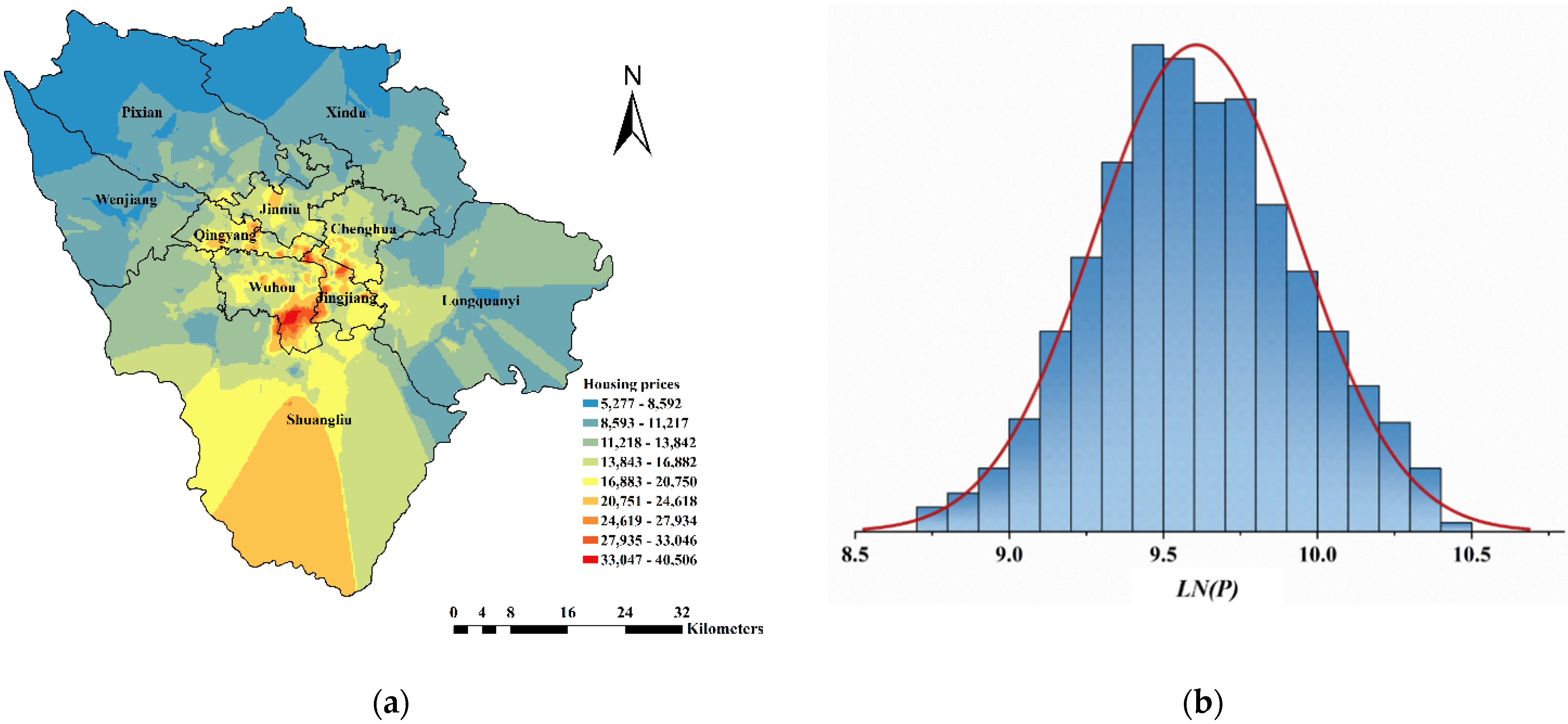
Chengdu, the capital of Sichuan province, is the study area. Chengdu is one of the political, financial, and transportation centers of Southwest China and had a GDP of 1700 billion yuan and a population of 16 million in 2019 [43]. The exciting culture, pleasant environment, and abundant presence of historical sites attract a large number of tourists to Chengdu every year. The solid economic foundation and the developed tourism industry have promoted UR development in Chengdu. The study area includes nine municipal districts of Chengdu: Wuhou, Qingyang, Shuangliu, Qingyang, Wenjiang, Pidu, Longquanyi, and Jinniu (Figure 1a).

3.2. Data and Variables

3.2.1. Dependent Variables

As the second-hand housing market exhibits a considerably more dispersed and large-scale housing supply compared with the new housing market [44], this study obtains second-hand house transaction data from Fangtuanxia (fangtianxia.com), one of the largest house intermediary platforms in China. This dataset reports information regarding housing prices, housing size, the presence of elevators, the floor area ratio, and the level of property management. To make the data comparable, this study does not consider villas and townhouses, which command an obviously high housing price and only account for 2.3% of the total samples and selects the multi-layer and high-rise housings as the major research object. In addition, differences within a residential community are ignored, and the data of houses attributed to the same community are merged [45]. Therefore, the average housing prices of residential neighborhoods are used as the dependent variables. After the above treatment and removing abnormal values, the final dataset includes 73,889 houses and 2286 residential communities. The Kriging method [46] is used for the spatial interpolation of housing prices. The results are split into nine levels based on the Jenks classification. Figure 1a represents the spatial distribution of Chengdu housing prices, which is characterized by a circular distribution. The housing prices decrease from the city center to the city boundaries; the highest housing prices are in the city center area, and lower price houses are mainly distributed in Northwest Chengdu. The housing prices of Tianfu New District show a rapid growth trend due to policy support. The housing prices of Chengdu have begun to shift from a unipolar distribution centered on Tianfu Square to a bipolar distribution. In addition, the logarithm of Chengdu housing price (LN(P)) is approximately normally distributed (Figure 1b), and the mean of LN(P) is 9.61.

3.2.2. Independent Variables

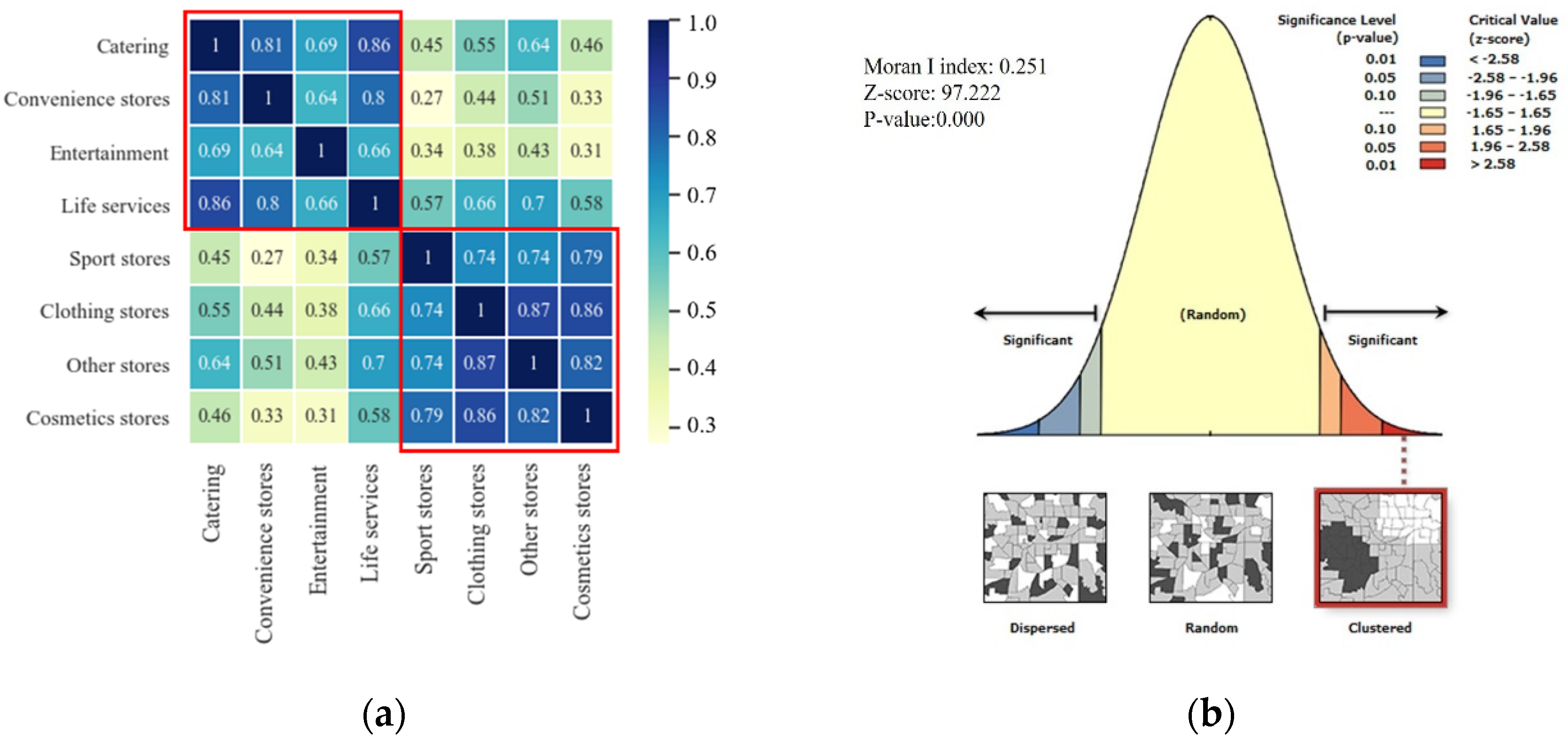
Urban retail refers to all consumer-related activities. Based on the classification rules of the Gaode Map, this study selected eight urban retail store categories, including catering stores, convenience stores, entertainment stores, life services stores, sport stores, clothing stores, cosmetics stores, and other stores (Figure 2a), and uses a number of these stores within 500 m of the house. Meanwhile, mega markets (e.g., shopping malls) are broken up into multiple independent urban retail stores, to be counted separately.

A correlation analysis (Figure 2a) reveals that the different UR types are significantly correlated, and all the correlations are positive (most values exceed 0.4). Catering, clothing stores, and other stores are strongly correlated with almost all other UR types. In addition, there are two clusters: (1) catering, convenience stores, entertainment, and life services, and (2) sport stores, clothing stores, other stores, and cosmetics stores. When the UR density of an area reaches a certain level, the area may be considered a commercial area. Meanwhile, the Moran I index of UR is 0.251 and is significant at the 95% level (Figure 2b), which indicates a space-clustered distribution of UR. Furthermore, excessive correlation generates multicollinearity in the regression analysis. Therefore, the total number of stores of different UR types is used as a UR-related variable.

For control variables, consumers’ demands for the functional characteristics of a house affect their willingness to pay [36]. Therefore, based on past research and residents’ demands, we employ control variables from six dimensions (housing structural characteristics, education, transport, medical, environment, and others). Independent variables are divided into structural variables, surrounding variables, and environmental variables [47]. Property management (PM) and school district (SD) are the scores assessed by real estate agency websites (Fangtianxia). The assessment of property management follows the standard of property management service grade of residential building, which classifies property management into four grades depending on the degree of building management, maintenance of shared facilities and equipment, maintenance of public order, and cleaning services. The assessment of school districts is decided by the rank of the supporting primary school and junior middle school of the house. A higher number indicates a better quality of property management and school district. The distances between houses and independent variables may take two forms: real distances (in the road network) and Euclidean distances. Among them, the distances to senior high school (DSHS), university (DUN), subway station (DSUB), hospital (DHOS) and park or square (DG) are real distances. The distance to the urban center (DUC) is based on Euclidean distance; DUC is not used in this study to describe the accessibility of the facility but the location of houses.

Table 1. Independent variables and descriptions.

Category	Variable	Abbreviation	Description
Dependent variable	Residential housing prices	P	Price per square meter (yuan/m2)
Structural variables	Size	SIZE	Area of structure (m2)
	Year	YEAR	The age of the house
	Elevator	EL	If the residence is equipped with elevator, 0 = no; 1 = yes
	Plot ratio	PR	Floor Area Ratio/Volume Fraction (%)
	Property management	PM	0 = Needs improvement; 1 = Low; 2 = Mid; 3 = High
Location variables	Urban Retail	UR	The number of relevant stores within 500 m
	School district	SD	0 = Low; 1 = Mid; 2 = High
	Kindergarten	KG	The number of kindergartens within 1000 m
	Distance to senior high school	DSHS	The real distance (not Euclidean distance) to the nearest public senior high school
	Distance to university	DUN	The real distance (not Euclidean distance) to the nearest university
	Bus station	BUS	The number of bus stations within 500 m
	Distance to subway station	DSUB	The real distance (not Euclidean distance) to the nearest subway station
	Distance to hospital	DHOS	The real distance (not Euclidean distance) to the nearest comprehensive hospital
	Distance to urban center	DUC	The distance (Euclidean distance) to Tianfu Square
Environment variables	Distance to park or square	DG	The real distance (not Euclidean distance) to the parks or squares

lists the community-level independent housing variables and relevant descriptions.

3.3. Methods

The hedonic price model is typically used to analyze the relationships between housing prices and housing characteristics. It may take different forms: linear, semi-log, and log–log. No theory determines the choice of the functional form. A previous study suggests that log-form models reduce heteroscedasticity [48]. In this study, the discrete variables (EL, YEAR, PM and SD) adopt the original form, and other variables are logarithmized (Equation (1)).

$$LN\left(P\right)={\beta }_0+{\beta }_{1}LN\left(UR\right)+{\beta }_{4}LN\left(S\right)+{\beta }_{5}LN\left(L\right)+{\beta }_{6}LN\left(E\right)+{\beta }_{7}Z+\epsilon$$

(1)

where P indicates housing prices, UR is the UR level surrounding the house, $\beta$ indicates the regression coefficient, S comprises continuous structural variables, L indicates continuous location variables, E comprises continuous environment variables, Z indicates other continuous-discrete variables, and ε is the error term.

In Chinese, the design of urban residential buildings must follow the standards of sound insulation. These standards of sound insulation have been revised many times to improve sound insulation performance. For example, non-standard before 2000, codes for sound insulation design of residential buildings were introduced in 2010 and 2020. Therefore, we assume building age has a positive relationship with building performance of sound insulation and use YEAR to characterize building performance of sound insulation. The interaction items ($LN\left(UR\right)\times PM$, $LN\left(UR\right)\times YEAR$) are introduced in the model to explore the moderating effect of housing structural characteristics (Equation (2)).

$$\begin{array}{c}LN\left(P\right)={\beta }_0+{\beta }_{1}LN\left(UR\right)+{\beta }_2\left(LN\left(UR\right)\times PM\right)+{\beta }_3\left(LN\left(UR\right)\times YEAR\right)\\ +{\beta }_{4}LN\left(S\right)+{\beta }_{5}LN\left(L\right)+{\beta }_{6}LN\left(E\right)+{\beta }_{7}Z+\epsilon \end{array}$$

(2)

Quantile Regression is used to test the residents’ demands on UR from price quantile. Quantile Regression estimators are calculated based on asymmetric absolute residual minimization. Compared with the hedonic price model, quantile regression has some advantages: (1) it does not require strong assumptions for the error terms and the estimation results are robust to outliers; and (2) it describes the whole conditional distribution of explained variables more comprehensively [36]. The regression coefficients across different housing price levels are obtained as follows:

$$LN\left(P\right)={\beta }_{0\left(q\right)}+{\beta }_{1\left(q\right)}LN\left(UR\right)+{\beta }_{4\left(q\right)}LN\left(S\right)+{\beta }_{5\left(q\right)}LN\left(L\right)+{\beta }_{6\left(q\right)}LN\left(E\right)+{\beta }_{7\left(q\right)}Z+\epsilon$$

(3)

where q indicates housing price quantiles; ${\beta }_{0\left(q\right)}$, ${\beta }_{1\left(q\right)}$, ${\beta }_{4\left(q\right)}$, ${\beta }_{5\left(q\right)}$, ${\beta }_{6\left(q\right)}$ and ${\beta }_{7\left(q\right)}$ are the qth quantile coefficients to be estimated; and the remaining variables are the same as in Equation (1).

An urban housing market, which usually comprises various submarkets, is too complex to be described as a spatially homogeneous unit [13,49]. Tobler’s First Law of Geography indicates that there are more similarities between adjacent geographical entities. Due to the uneven distribution of urban retail resources and other housing characteristics, there may be spatial heterogeneity in the resident’s demands for UR. The global regression of the hedonic pricing model is not detailed enough to explain the local conditions. The geographically weighted regression model uses the local smooth processing method to solve the problem of spatial heterogeneity. Considering spatial heterogeneity, geographic coordinates and core functions are utilized to carry out local regression estimation on the adjacent individuals of each group. Therefore, this study tests the spatial heterogeneity of the capitalization effects of UR on housing prices based on the result of the geographically weighted regression model, as follows:

$$LN\left(P_i\right)={{\displaystyle \sum }}_j{\beta }_{ij}\left({\mu }_i,v_i\right)X_{ik}+{\epsilon }_i$$

(4)

where $\left({\mu }_i,v_i\right)$ indicates the spatial location of sample house i, and $\beta \left({\mu }_i,v_i\right)$ is the regression coefficient on sample house i. In contrast with the hedonic price model, a weighted matrix $W_i$ is used to indicate the influence of different observation points with different spatial locations on the estimation of the coefficient of sample house i [50]. In this study, we use the Gaussian function to calculate the weighted matrix, as follows.

$$W_{ij}=e^{-\frac{1}{2}{\left(\frac{d_{ij}}{b}\right)}^2}$$

(5)

where $d_{ij}$ indicates the Euclidean distance from sample house i to observation house j, b indicates the bandwidth, and the selection of b follows the AICc criterion [50].

4. Results and Discussion

4.1. Hedonic Price Model Results

Table 2. Baseline hedonic price model results.

Variable	Model (1)				Model (2)
	Coefficient	SE	p Value	VIF	Coefficient	SE	p Value	VIF
LN(UR)	−0.051 ***	0.009	0.000	1.897	−0.053 ***	0.008	0.000	1.985
LN(UR)$\times$PM					0.020 **	0.013	0.092	2.357
LN(UR)$\times$YEAR					−0.003 **	0.002	0.042	2.357
PM	0.085 ***	0.011	0.000	2.927	0.083 ***	0.012	0.000	3.003
YEAR	−0.014 ***	0.001	0.000	3.745	−0.014 ***	0.001	0.000	3.755
EI	0.080 ***	0.014	0.000	2.108	0.081 ***	0.014	0.000	2.128
LN(BUS)	0.051 ***	0.016	0.002	2.491	−0.035 ***	0.006	0.002	2.492
LN(DSUB)	−0.036 ***	0.006	0.000	1.227	−0.035 ***	0.006	0.000	1.233
LN(DUC)	−0.279 ***	0.008	0.000	1.881	−0.281 ***	0.008	0.000	1.917
LN(DG)	0.004	0.006	0.478	1.190	0.005	0.006	0.449	1.193
LN(DHOS)	0.042 ***	0.006	0.000	1.411	0.042 ***	0.006	0.000	1.413
LN(KD)	0.132 ***	0.019	0.000	3.210	0.130 ***	0.019	0.000	3.221
LN(DUN)	0.037 ***	0.006	0.000	1.270	0.037 ***	0.006	0.000	1.271
LN(DSHS)	−0.024 *	0.014	0.088	1.014	−0.024 *	0.014	0.081	1.015
SD	0.034 ***	0.009	0.000	1.078	0.034 ***	0.009	0.000	1.079
PR	0.010 ***	0.003	0.001	1.222	0.010 ***	0.003	0.001	1.224
LN(SIZE)	0.163 ***	0.016	0.000	1.113	0.161 ***	0.016	0.000	1.116
Intercept	10.903 ***	0.189	0.000		10.551 ***	0.274	0.000
Adjusted R2	0.560				0.564

Note: ***, **, and * represent 1%, 5%, and 10% significance levels, respectively. SE represents standard error of regression coefficient. VIF represents variance inflation factor, which is used to quantify the degree of multicollinearity.

represents the baseline hedonic price model results for the capitalization effect of UR on housing prices in all districts. Model (2) introduces the two interaction items. All the adjusted R² values exceed 0.5, indicating that the model explains over 50% of the variation in housing prices. Most regression coefficients are significant at the 5% level. Hence, the proposed hedonic price model has adequate explanatory power.

The results of Model (1) indicate that UR had a negative effect on housing prices in all districts. The regression coefficient of UR is −0.051 at the 1% significance level, indicating that a 1% increase in UR is associated with a 0.051% decrease in housing prices. This result indicates that residents were more sensitive to the negative influences of UR compared to the convenience of UR, which makes them reject the increase in UR density.

For the results of Model (2), the regression coefficient of UR is similar to that of Model (1). The regression coefficient of the interaction item of UR and property management is at the 10% significance level (p-value = 0.092) and the value is 0.020. This indicates that property management has a positive moderating effect on the capitalization effect of UR on housing prices. Generally, the negative effect of UR on housing prices decreases as the quality of property management increases. For the interaction item of UR and building age, the coefficient is −0.003 at the 10% significance level, indicating that the negative effect of UR on housing price decreases with improvements in performance of building sound insulation (as the building age decreases). These results are consistent with the fact that property management and performance of building sound insulation (YEAR) can reduce the residents’ perception that UR has a negative influence on environment and society [51,52]. The negative impact of UR on residents’ quality of life usually decreases residents’ preference for UR, which leads the demand curve to move to the left and the premium of UR to decrease. However, greater property management means better security, which can keep the community isolated from strangers to the maximum extent possible and decrease the potential probability of crime [52]. Furthermore, new buildings usually adopt better construction technologies and construction materials to improve performance of building sound insulation, which effectively insulate residents from adverse environments and create a more comfortable living experience for residents [53]. Therefore, compared with the owners who have housing with bad sound insulation, the demand curve of owners having houses with good sound insulation is further to the right. In other words, they are willing to pay a higher premium for UR.

Meanwhile, the coefficient of PM is 0.083 at the 1% significance level (the results of Model 1 and Model 2 are approximately the same), which means that property management and building have a direct capitalization effect on housing prices. Further, the coefficient of YEAR is −0.014 at the 1% significance level, indicating that newer housing with better performance of building sound insulation are preferred by home-buyers. Therefore, considering the double effect of property management and performance of building sound insulation, developers can achieve higher premiums by adopting better property management services and construction techniques, particularly for houses in areas with high UR density. Moreover, there is little difference in the control variables’ regression coefficients of Model (1) and Model (2), confirming their robustness.

4.2. Quantile Regression Results

The baseline results of the hedonic price model are reported in Column 1 of

Table 3. Quantile regression results.

Variable	(1)	(2)	(3)	(4)	(5)	(6)	(7)	(8)	(9)	(10)
	Global	Q10	Q20	Q30	Q40	Q50	Q60	Q70	Q80	Q90
LN(UR)	−0.051 ***	0.012 ***	0.006 **	−0.028 ***	−0.045 ***	−0.057 ***	−0.063 ***	−0.079 ***	−0.076 ***	−0.093 ***
	(0.008)	(0.004)	(0.003)	(0.010)	(0.010)	(0.009)	(0.010)	(0.011)	(0.012)	(0.017)
EI	0.080 ***	0.094 ***	0.080 ***	0.079 ***	0.079 ***	0.079 ***	0.074 ***	0.079 ***	0.093 ***	0.071 **
	(0.014)	(0.024)	(0.019)	(0.018)	(0.017)	(0.016)	(0.017)	(0.020)	(0.022)	(0.030)
YEAR	−0.014 ***	−0.007 ***	−0.012 ***	−0.015 ***	−0.015 ***	−0.014 ***	−0.016 ***	−0.015 ***	−0.015 ***	−0.016 ***
	(0.001)	(0.002)	(0.002)	(0.002)	(0.002)	(0.002)	(0.002)	(0.002)	(0.002)	(0.003)
LN(BUS)	0.051 ***	0.047 *	0.046 **	0.049 **	0.048 **	0.038 **	0.051 **	0.042 *	0.067 ***	0.055
	(0.016)	(0.028)	(0.022)	(0.021)	(0.020)	(0.019)	(0.020)	(0.023)	(0.025)	(0.035)
LN(DSUB)	−0.036 ***	−0.047 ***	−0.038 ***	−0.031 ***	−0.031 ***	−0.035 ***	−0.048 ***	−0.047 ***	−0.046 ***	−0.030 **
	(0.006)	(0.010)	(0.008)	(0.008)	(0.007)	(0.007)	(0.008)	(0.009)	(0.009)	(0.013)
LN(DUC)	−0.279 ***	−0.243 ***	−0.264 ***	−0.277 ***	−0.284 ***	−0.290 ***	−0.291 ***	−0.286 ***	−0.286 ***	−0.303 ***
	(0.008)	(0.013)	(0.010)	(0.010)	(0.009)	(0.009)	(0.010)	(0.011)	(0.012)	(0.017)
LN(DG)	0.004	0.015	0.019**	0.016**	0.013*	0.007	−0.001	−0.004	−0.013	0.011
	(0.006)	(0.011)	(0.008)	(0.008)	(0.007)	(0.007)	(0.008)	(0.009)	(0.010)	(0.013)
LN(DHOS)	0.042 ***	0.030 ***	0.041 ***	0.041 ***	0.045 ***	0.048 ***	0.043 ***	0.051 ***	0.045 ***	0.041 ***
	(0.006)	(0.010)	(0.008)	(0.007)	(0.007)	(0.007)	(0.007)	(0.008)	(0.009)	(0.013)
LN(KD)	0.132 ***	0.086 ***	0.105 ***	0.129 ***	0.157 ***	0.168 ***	0.153 ***	0.153 ***	0.133 ***	0.130 ***
	(0.019)	(0.032)	(0.025)	(0.024)	(0.023)	(0.022)	(0.023)	(0.027)	(0.029)	(0.041)
LN(DUN)	0.037 ***	0.041 ***	0.033 ***	0.037 ***	0.039 ***	0.037 ***	0.037 ***	0.032 ***	0.047 ***	0.045 ***
	(0.006)	(0.011)	(0.008)	(0.008)	(0.007)	(0.007)	(0.008)	(0.009)	(0.010)	(0.013)
LN(DSHS)	−0.024 *	−0.033	−0.014	−0.010	−0.011	−0.009	−0.011	−0.021	−0.025	−0.033
	(0.014)	(0.023)	(0.018)	(0.017)	(0.016)	(0.016)	(0.017)	(0.019)	(0.021)	(0.030)
SD	0.034 ***	0.030 *	0.022 *	0.030 ***	0.032 ***	0.030 ***	0.028 **	0.043 ***	0.044 ***	0.045 **
	(0.009)	(0.016)	(0.012)	(0.012)	(0.011)	(0.011)	(0.011)	(0.013)	(0.014)	(0.020)
PR	0.010 ***	0.007	0.007*	0.008 **	0.007 **	0.010 ***	0.010 ***	0.010 **	0.009 *	0.010
	(0.003)	(0.005)	(0.004)	(0.004)	(0.004)	(0.003)	(0.004)	(0.004)	(0.005)	(0.006)
PM	0.085 ***	0.089 ***	0.072 ***	0.063 ***	0.078 ***	0.086 ***	0.086 ***	0.077 ***	0.095 ***	0.086 ***
	(0.011)	(0.019)	(0.015)	(0.014)	(0.014)	(0.013)	(0.014)	(0.016)	(0.018)	(0.025)
LN(SIZE)	0.163 ***	0.088 ***	0.106 ***	0.150 ***	0.168 ***	0.157 ***	0.184 ***	0.186 ***	0.194 ***	0.248 ***
	(0.016)	(0.026)	(0.021)	(0.020)	(0.019)	(0.018)	(0.019)	(0.022)	(0.024)	(0.033)
_cons	10.903 ***	10.780 ***	10.734 ***	10.613 ***	10.540 ***	10.699 ***	10.940 ***	11.031 ***	11.082 ***	11.026 ***
	(0.189)	(0.319)	(0.249)	(0.237)	(0.224)	(0.219)	(0.232)	(0.265)	(0.288)	(0.403)
Pseudo R2	-	0.347	0.357	0.360	0.364	0.368	0.367	0.360	0.351	0.326
Adjusted R2	0.563	-	-	-	-	-	-	-	-	-
N	2286	2286	2286	2286	2286	2286	2286	2286	2286	2286

Note: ***, **, and * represent 1%, 5%, and 10% significance levels, respectively.

for comparison. The full quantile regression includes eight estimates from the 20th quantile to the 90th quantile and specifies the capitalization effect of UR on different levels of housing prices.

Table 3 lists the quantile regression results. The pseudo R² of all the quantiles is between 0.326 and 0.368, indicating that all models have adequate explanatory power. All the regression coefficients of LN(UR) are significant at the 1% level, indicating that UR has a capitalization effect on all levels of housing prices. However, the capitalization effect on different levels of housing prices is significantly different in heterogenous price quantiles. Specifically, with the increase in housing prices, the coefficients decrease from 0.012 to −0.093. UR also shows a positive and negative effect on low-price houses (Q10 and Q20) and medium-/high-price houses (Q30–Q90), respectively. In other words, the owners of low-price houses represent positive demands on UR, and the owners of high-price houses resist the increase in UR density.

This result be due to various reasons. First, compared to high-price houses, UR development is lower in the surroundings of low-price houses. Those living in low-price houses may not be as mobile as the residents of high-price neighborhoods [53]. For example, the owners of high-price houses usually own more private cars and are less sensitive to increases in transportation costs [42]. Therefore, there might be lower demand from the owners of high-price houses for the convenience of UR service near their houses. In addition, wealthier residents tend to be more concerned about the privacy and comfort of their homes [20]. More UR stores imply increased adverse impacts on the environment, such as noise pollution, large crowds, trash accumulation, and increased crime rate due to the presence of strangers [13]. The owners of high-price houses will show less tolerability to the negative influence of UR than those who own low- and medium-price houses. In addition, more job opportunities from high density UR areas may also lead to gaps between the demands of the owners of low-price and high-price houses [6]. The above reasons meant that the demand curve of high-price house owners were more to the left than the demand curve of low-price house owners. In other words, high-price house owners are willing to pay a lower premium for UR.

4.3. Geographically Weighted Regression Model Results

Before building a spatial econometric model of Chengdu housing prices, we test the spatial autocorrelation of the logarithm of housing prices. The Moran I index of logarithm of housing is 0.576 at the 1% significance level (p-values < 0.01), indicating that Chengdu housing prices are characterized by positive spatial autocorrelation and spatial aggregation (the high-price houses are clustered together, as are the low-price houses). Hence, the geographically weighted regression model is used to estimate the spatial heterogeneity of the impact of the above-mentioned explanatory variables on housing prices in Chengdu. Because the regression of coefficients of distance to park or square are not significant in global and all price quantiles, we remove distance to park or square in the geographically weighted regression model.

Table 4. Results of geographically weighted regression model.

Variable	Max	Median	Min	Mean
LN(UR)	0.2009	−0.0407	−0.8097	−0.0779
EI	0.2613	0.1276	−0.0526	0.1289
YEAR	0.0098	−0.2566	−0.8356	−0.2699
LN(BUS)	0.3468	0.0585	−0.2544	0.0562
LN(DSUB)	0.1343	−0.0415	−0.3572	−0.0392
LN(DUC)	0.5170	−0.6877	−2.4070	−0.6817
LN(DHOS)	0.7616	0.1374	−0.6634	0.1034
LN(KD)	0.2712	0.0114	−0.2021	0.0171
LN(DUN)	1.5305	0.0077	−1.6244	0.0519
LN(DSHS)	0.2499	0.0281	−0.4133	0.0203
SD	0.2027	−0.0037	−0.2645	0.0011
PR	0.4484	0.1332	−0.1476	0.1350
PM	0.2955	0.1254	−0.0812	0.1196
LN(SIZE)	1.9464	0.2349	−0.7878	0.2602
Intercept	0.2009	−0.0407	−0.8097	−0.0779
Bandwidth	60 2286 0.775
N
Adjusted R2

presents the minimum, median, maximum, and mean of geographically weighted regression model results. The adjusted R² of the geographically weighted regression model is 0.775, significantly higher than the hedonic price model (0.560), indicating superior explanatory power. Spatial heterogeneity has a significant impact on the capitalization effect of UR on housing prices. The regression coefficients of LN(UR) show both positive and negative values, indicating that residents’ demands for UR are significantly different in different regions and represents demand and rejection simultaneously.

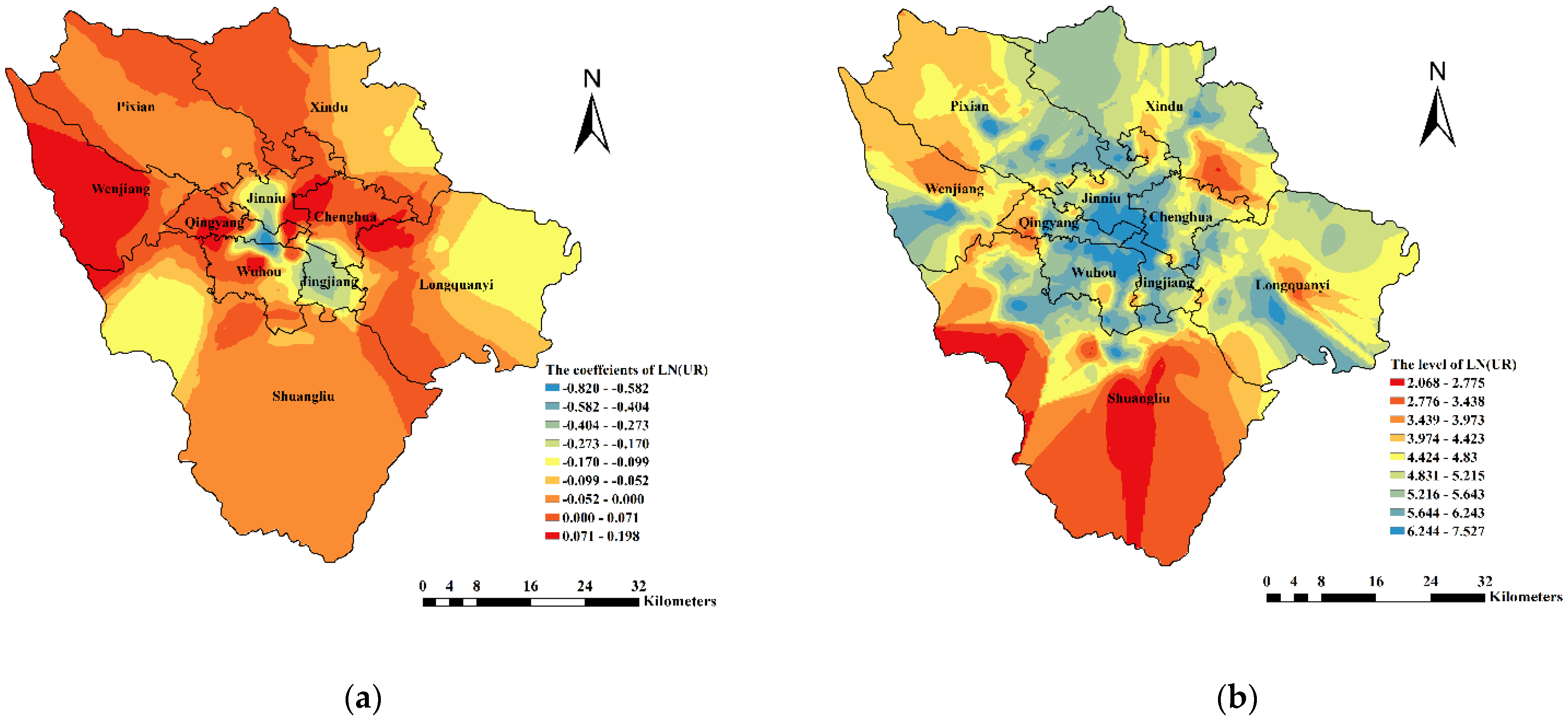
To further examine the influence of spatial heterogeneity, we employ the Kriging method (Figure 3a) to perform spatial interpolation on the coefficients of LN(UR). Negative coefficients were observed in the core area of Chengdu, with Tianfu Square as the center, while positive coefficients were observed in the peripheral area of Chengdu, particularly in Wenjiang and Pixian districts, which are in the northwest area of Chengdu. In general, the coefficients of LN(UR) show significant spatial heterogeneity and reflect a nearly circular distribution, which gradually increases outward from the city center (from −0.8097 to 0.2009). In other words, residents in the periphery area need an increased UR intensity to realize convenience from UR, and residents in the core area reject the increase in UR intensity to protect their habitable environment and life equality.

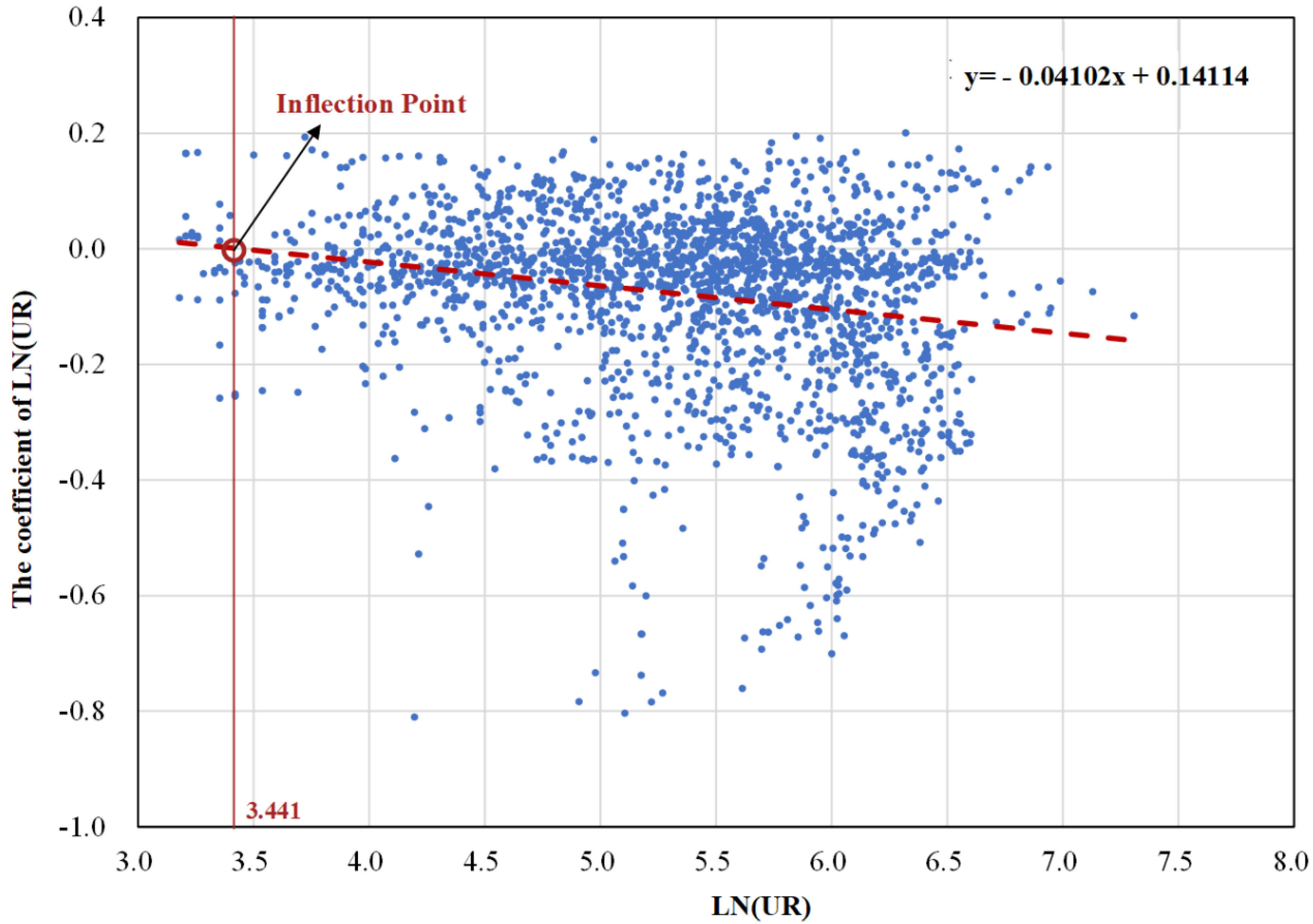
Furthermore, we plot the spatial distribution of LN(UR) (Figure 3b) and assign a reverse color direction (the blue part indicates higher ownership LN(UR)) for ease of comparison with Figure 3a. We find that the LN(UR) coefficients have a similar spatial distribution to LN(UR). Hence, we assume that the regression coefficient of LN(UR) is related to the level of LN(UR). This hypothesis is supported by the scatter diagram (Figure 4) between the LN(UR) and coefficients of LN(UR). Figure 4 shows that LN(UR) has a negative impact on the regression coefficients of LN(UR), which implies that the positive capitalization effect of LN(UR) on housing prices gradually decreases with the increase in the level of LN(UR). The fitting straight line indicates that the impact of average LN(UR) on housing prices shifts from promotion to inhibition when average LN(UR) reaches 3.441, where the attitude of residents changes from demand to resistance. This shows that there is an inverted U-shaped relationship between LN(UR) and housing prices. To directly confirm this deduction, we established a new hedonic price model, which introduced the square of LN(UR). The result is shown in

Table A1. The results of the hedonic price model with LN(UR)².

Variable	Model (1)				Model (3)
	Coefficient	SE	p Value	VIF	Coefficient	SE	p Value	VIF
LN(UR)	−0.051 ***	0.009	0.000	1.897	0.107	0.068	0.117	134.689
LN(UR)2					−0.015 **	0.007	0.020	133.717
PM	0.085 ***	0.011	0.000	2.927	0.085 ***	0.011	0.000	2.928
YEAR	−0.014 ***	0.001	0.000	3.745	−0.014 ***	0.001	0.000	3.745
EI	0.080 ***	0.014	0.000	2.108	0.079 ***	0.014	0.000	2.113
LN(BUS)	0.051 ***	0.016	0.002	2.491	−0.051 ***	0.016	0.002	2.491
LN(DSUB)	−0.036 ***	0.006	0.000	1.227	−0.035 ***	0.006	0.000	1.228
LN(DUC)	−0.279 ***	0.008	0.000	1.881	−0.282 ***	0.008	0.000	1.905
LN(DG)	0.004	0.006	0.478	1.19	0.004	0.006	0.520	1.191
LN(DHOS)	0.042 ***	0.006	0.000	1.411	0.042 ***	0.006	0.000	1.412
LN(KD)	0.132 ***	0.019	0.000	3.21	0.127 ***	0.019	0.000	3.247
LN(DUN)	0.037 ***	0.006	0.000	1.27	0.037 ***	0.006	0.000	1.27
LN(DSHS)	−0.024 *	0.014	0.088	1.014	−0.024 *	0.014	0.085	1.014
SD	0.034 ***	0.009	0.000	1.078	0.034 ***	0.009	0.000	1.079
PR	0.010 ***	0.003	0.001	1.222	0.010 ***	0.003	0.001	1.228
LN(SIZE)	0.163 ***	0.016	0.000	1.113	0.163 ***	0.016	0.000	1.113
Intercept	10.903 ***	0.189	0.000		10.551 ***	0.244	0.000
Adjusted R2	0.560				0.561

Note: ***, **, and * represent 1%, 5%, and 10% significance levels, respectively.

. From Table A1, we can see that the regression coefficients of the square of LN(UR) was −0.015 at the 5% significance level, confirming the inverted U-shaped relationship between LN(UR) and housing prices. Generally, before LN(UR) reaches the inflection point, LN(UR) has a positive capitalization effect on housing prices, which decreases with the increase of LN(UR). After reaching the inflection point, the positive capitalization effect changes to a negative effect on housing prices. This might be due to two reasons: (1) with the increase in UR, the demand for the convenience of UR eventually plateaus, which leads to a reduction in the willingness to pay for the increase of UR convenience and (2) the increase in UR will attract more consumers and negatively affect the comfort of the living environment [10,13].

5. Conclusions

An accurate understanding of the residents’ demands for UR in heterogeneous conditions is crucial for the UR layout of cities. Based on the second-hand housing transaction data of Chengdu, this study employed the hedonic price model, quantile regression, and geographically weighted regression to explore the capitalization effect of urban retail on housing prices and the gap between residents’ demands for UR in heterogeneous housing characteristics, heterogeneous price quantiles, and heterogeneous space. The main results are as follows: (1) The level of property management (PM) and house age (YEAR) have a moderating effect on the capitalization effect of UR on housing prices. Specifically, good property management and good sound insulation can decrease the negative influence of UR on residents’ lives; (2) The owners of high-price houses have a lower demand for UR compared to the owners of low-price houses; (3) The capitalization effect of UR on housing prices is spatially heterogeneous and decreases as we move outward from the Chengdu central area to the Chengdu peripheral area; (4) There is an inverted U-shaped relationship between UR and housing prices.

In contrast with previous studies, this study is the first to discuss the inverted U-shaped relationship between housing prices and UR and to analyze the moderating effect of housing structure characteristics on residents’ demand for UR. These research perspectives can provide some reference for further studies on housing prices, such as the relationship between transportation infrastructure and housing prices. For practice, this study also provides several policy implications for real-estate developers and city planning departments. First, considering the negative impact of UR on residents’ lives, the city planning department should prevent excessive urban retail development in developed areas, which, with a high UR intensity or older houses, focuses on regional security and environmental management to offset the negative impacts of UR. Specifically, the results of geographically weighted regression indicate that Wenjian and Xindu are more appropriate for UR development. On the contrary, Wuhou, Jingjiang and Jinniu should try to decrease their UR density. Furthermore, because of the local regression of geographically weighted regression, according to the regression coefficients of houses with similar environments and location variables, planer can find the UR development limitation of a specific region. The inverted U-shaped curve indicates that the UR intensity of a dwelling district should not be more than 125/km² (exp(3.441)/0.5²). Meanwhile, actively developing the UR in boundary areas that have lower UR intensity can improve the quality of life of local residents and relieve the pressure on existing commercial areas. Second, real-estate developers should fully focus on consumers’ characteristics and adopt different real estate development strategies. Specifically, for consumers with high incomes, real-estate developers should pay more attention to the establishment of a livable and private living environment, since these consumers are not sensitive to the convenience derived from UR. On the contrary, the convenience derived from UR and reducing the travel cost should be the focus of real-estate developers for consumers with low incomes as the major target consumer group. In addition, by considering the direct and indirect positive impacts of suitable property management and the performance of building sound insulation on housing prices, real-estate developers should consider adopting better property management and sound insulation to increase housing prices, especially in areas with high UR intensity.

This study has some limitations. First, it only focuses on the real-estate market in 2019 without considering changes in the capitalization effect of UR on housing prices over time. Therefore, residents’ demands for UR at different times remains unclear. For example, in the past, residents needed to reach retail stores for accessing UR activities. Now, residents can enjoy various services without leaving their homes through online shopping platforms such as Meituan and Taobao. Online UR reduces the need for physical UR resources. Future studies should employ a space–time econometric model and consider variables related to online business. Second, given the strong correlation between different types of UR, this study merges all UR types. Hence, the impacts of different UR types on housing prices and residents’ demands for different UR types (such as catering, auto service, and clothing sales, among others) are not considered. Finally, because of the limitations of our data, this study does not further discuss the relationship between the residents’ demand for urban retail and the employment capacity created by retail, especially for rural areas. These may have some implications for government retail layout plans. Future research should discuss these questions, providing guidance for the optimization of regional internal UR structures.

References

- Song, Y.; Sohn, J. Valuing spatial accessibility to retailing: A case study of the single family housing market in Hillsboro, Oregon. J. Retail. Consum. Serv. 2007, 14, 279–288. [Google Scholar] [CrossRef]
- Andersson, D.E.; Shyr, O.F.; Fu, J. Does high-speed rail accessibility influence residential property prices? Hedonic estimates from southern Taiwan. J. Transp. Geogr. 2010, 18, 166–174. [Google Scholar] [CrossRef]
- Sander, H.; Polasky, S.; Haight, R.G. The value of urban tree cover: A hedonic property price model in Ramsey and Dakota Counties, Minnesota, USA. Ecol. Econ. 2010, 69, 1646–1656. [Google Scholar] [CrossRef]
- Geng, B.; Bao, H.; Liang, Y. A study of the effect of a high-speed rail station on spatial variations in housing price based on the hedonic model. Habitat Int. 2015, 49, 333–339. [Google Scholar] [CrossRef]
- Wu, C.; Ye, X.; Du, Q.; Luo, P. Spatial effects of accessibility to parks on housing prices in Shenzhen, China. Habitat Int. 2017, 63, 45–54. [Google Scholar] [CrossRef]
- Cho, J.; Chun, H.; Lee, Y. How does the entry of large discount stores increase retail employment? Evidence from Korea. J. Comp. Econ. 2015, 43, 559–574. [Google Scholar] [CrossRef]
- Colaço, R.; De Abreu e Silva, J. Commercial Classification and Location Modelling: Integrating Different Perspectives on Commercial Location and Structure. Land 2021, 10, 567. [Google Scholar] [CrossRef]
- Erkip, F.; Kızılgün, Ö.; Akinci, G.M. Retailers’ resilience strategies and their impacts on urban spaces in Turkey. Cities 2014, 36, 112–120. [Google Scholar] [CrossRef] [Green Version]
- Jang, M.; Kang, C.-D. Retail accessibility and proximity effects on housing prices in Seoul, Korea: A retail type and housing submarket approach. Habitat Int. 2015, 49, 516–528. [Google Scholar] [CrossRef]
- Zhang, L.; Zhou, J.; Hui, E.C.; Wen, H. The effects of a shopping mall on housing prices: A case study in Hangzhou. Int. J. Strateg. Prop. Manag. 2019, 23, 65–80. [Google Scholar] [CrossRef]
- Tang, L.; Lin, Y.; Li, S.; Li, S.; Li, J.; Ren, F.; Wu, C. Exploring the influence of urban form on urban vibrancy in shenzhen based on mobile phone data. Sustainability 2018, 10, 4565. [Google Scholar] [CrossRef] [Green Version]
- Yue, W.; Chen, Y.; Thy, P.T.M.; Fan, P.; Liu, Y.; Zhang, W. Identifying urban vitality in metropolitan areas of developing countries from a comparative perspective: Ho Chi Minh City versus Shanghai. Sustain. Cities Soc. 2021, 65, 102609. [Google Scholar] [CrossRef]
- Zhang, L.; Zhou, J.; Hui, E.C.-M. Which types of shopping malls affect housing prices? From the perspective of spatial accessibility. Habitat Int. 2020, 96, 102118. [Google Scholar] [CrossRef]
- Chiang, Y.-H.; Peng, T.-C.; Chang, C.-O. The nonlinear effect of convenience stores on residential property prices: A case study of Taipei, Taiwan. Habitat Int. 2015, 46, 82–90. [Google Scholar] [CrossRef]
- Tomal, M. Modelling housing rents using spatial autoregressive geographically weighted regression: A case study in Cracow, Poland. ISPRS Int. J. Geo-Inf. 2020, 9, 346. [Google Scholar] [CrossRef]
- Xiao, Y.; Hui, E.C.; Wen, H. Effects of floor level and landscape proximity on housing price: A hedonic analysis in Hangzhou, China. Habitat Int. 2019, 87, 11–26. [Google Scholar] [CrossRef]
- Saphores, J.-D.; Li, W. Estimating the value of urban green areas: A hedonic pricing analysis of the single family housing market in Los Angeles, CA. Landsc. Urban Plan. 2012, 104, 373–387. [Google Scholar] [CrossRef]
- Lu, J. The value of a south-facing orientation: A hedonic pricing analysis of the Shanghai housing market. Habitat Int. 2018, 81, 24–32. [Google Scholar] [CrossRef]
- Feng, H.; Lu, M. School quality and housing prices: Empirical evidence from a natural experiment in Shanghai, China. J. Hous. Econ. 2013, 22, 291–307. [Google Scholar] [CrossRef]
- Lee, H.; Lee, B.; Lee, S. The Unequal Impact of Natural Landscape Views on Housing Prices: Applying Visual Perception Model and Quantile Regression to Apartments in Seoul. Sustainability 2020, 12, 8275. [Google Scholar] [CrossRef]
- Tian, G.; Wei, Y.D.; Li, H. Effects of accessibility and environmental health risk on housing prices: A case of Salt Lake County, Utah. Appl. Geogr. 2017, 89, 12–21. [Google Scholar] [CrossRef]
- Pope, J.C. Fear of crime and housing prices: Household reactions to sex offender registries. J. Urban Econ. 2008, 64, 601–614. [Google Scholar] [CrossRef]
- Yusuf, A.A.; Resosudarmo, B.P. Does clean air matter in developing countries’ megacities? A hedonic price analysis of the Jakarta housing market, Indonesia. Ecol. Econ. 2009, 68, 1398–1407. [Google Scholar] [CrossRef]
- Yu, T.-H.; Cho, S.-H.; Kim, S.G. Assessing the Residential Property Tax Revenue Impact of a Shopping Center. J. Real Estate Financ. Econ. 2012, 45, 604–621. [Google Scholar] [CrossRef]
- Sirpal, R. Empirical modeling of the relative impacts of various sizes of shopping centers on the values of surrounding residential properties. J. Real Estate Res. 1994, 9, 487–505. [Google Scholar] [CrossRef]
- Sale, M. The impact of a shopping centre on the value of adjacent residential properties. Stud. Econ. Econom. 2017, 41, 55–72. [Google Scholar] [CrossRef]
- Suárez, A.; Del Bosque, I.R.G.; Rodríguez-Poo, J.M.; Moral, I. Accounting for heterogeneity in shopping centre choice models. J. Retail. Consum. Serv. 2004, 11, 119–129. [Google Scholar] [CrossRef]
- Earl, P.E.; Wakeley, T. Alternative perspectives on connections in economic systems. J. Evol. Econ. 2010, 20, 163–183. [Google Scholar] [CrossRef]
- Colwell, P.; Gujral, S.; Coley, C. The Impact of a Shopping Center on the Value of Surrounding Properties. Real Estate Issues 1985, 10, 35–39. [Google Scholar]
- Liu, Y.; Tang, Y. Epidemic shocks and housing price responses: Evidence from China’s urban residential communities. Reg. Sci. Urban Econ. 2021, 89, 103695. [Google Scholar] [CrossRef]
- Li, J.; Huang, H. Effects of transit-oriented development (TOD) on housing prices: A case study in Wuhan, China. Res. Transp. Econ. 2020, 80, 100813. [Google Scholar] [CrossRef]
- Bayer, P.; McMillan, R.; Rueben, K. An Equilibrium Model of Sorting in an Urban Housing Market; National Bureau of Economic Research: Cambridge, MA, USA, 2004. [Google Scholar] [CrossRef]
- Liao, W.-C.; Wang, X. Hedonic house prices and spatial quantile regression. J. Hous. Econ. 2012, 21, 16–27. [Google Scholar] [CrossRef]
- Koenker, R.W.; D’Orey, V. Algorithm AS 229: Computing regression quantiles. Appl. Stat. 1987, 36, 383–393. [Google Scholar] [CrossRef]
- Mak, S.; Choy, L.; Ho, W. Quantile regression estimates of Hong Kong real estate prices. Urban Stud. 2010, 47, 2461–2472. [Google Scholar] [CrossRef] [Green Version]
- Wen, H.; Xiao, Y.; Hui, E.C. Quantile effect of educational facilities on housing price: Do homebuyers of higher-priced housing pay more for educational resources? Cities 2019, 90, 100–112. [Google Scholar] [CrossRef]
- Wang, Y.; Feng, S.; Deng, Z.; Cheng, S. Transit premium and rent segmentation: A spatial quantile hedonic analysis of Shanghai Metro. Transp. Policy 2016, 51, 61–69. [Google Scholar] [CrossRef] [Green Version]
- Mueller, J.M.; Loomis, J.B. Does the estimated impact of wildfires vary with the housing price distribution? A quantile regression approach. Land Use Policy 2014, 41, 121–127. [Google Scholar] [CrossRef]
- Lin, Y.-J.; Chang, C.-O.; Chen, C.-L. Why homebuyers have a high housing affordability problem: Quantile regression analysis. Habitat Int. 2014, 43, 41–47. [Google Scholar] [CrossRef]
- Zhang, L. Flood hazards impact on neighborhood house prices: A spatial quantile regression analysis. Reg. Sci. Urban Econ. 2016, 60, 12–19. [Google Scholar] [CrossRef]
- Garza, N.; Ovalle, M.C. Tourism and housing prices in Santa Marta, Colombia: Spatial determinants and interactions. Habitat Int. 2019, 87, 36–43. [Google Scholar] [CrossRef]
- Fernandez, M.A.; Bucaram, S. The changing face of environmental amenities: Heterogeneity across housing submarkets and time. Land Use Policy 2019, 83, 449–460. [Google Scholar] [CrossRef]
- NBS (National Bureau of Statistic). Chinese Statistic Yearbook; China Statistic Press: Beijing, China, 2020. [Google Scholar]
- Qu, W.; Huang, Y.; Deng, G. Identifying the critical factors behind the second-hand housing price concession: Empirical evidence from China. Habitat Int. 2021, 117, 102442. [Google Scholar] [CrossRef]
- Liang, X.; Liu, Y.; Qiu, T.; Jing, Y.; Fang, F. The effects of locational factors on the housing prices of residential communities: The case of Ningbo, China. Habitat Int. 2018, 81, 1–11. [Google Scholar] [CrossRef]
- Gia Pham, T.; Kappas, M.; Van Huynh, C.; Hoang Khanh Nguyen, L. Application of ordinary kriging and regression kriging method for soil properties mapping in hilly region of Central Vietnam. ISPRS Int. J. Geo-Inf. 2019, 8, 147. [Google Scholar] [CrossRef] [Green Version]
- Grislain-Letrémy, C.; Katossky, A. The impact of hazardous industrial facilities on housing prices: A comparison of parametric and semiparametric hedonic price models. Reg. Sci. Urban Econ. 2014, 49, 93–107. [Google Scholar] [CrossRef] [Green Version]
- Wen, H.; Tao, Y. Polycentric urban structure and housing price in the transitional China: Evidence from Hangzhou. Habitat Int. 2015, 46, 138–146. [Google Scholar] [CrossRef]
- Bełej, M.; Cellmer, R.; Głuszak, M. The Impact of Airport Proximity on Single-Family House Prices—Evidence from Poland. Sustainability 2020, 12, 7928. [Google Scholar] [CrossRef]
- Brunsdon, C.; Fotheringham, A.S.; Charlton, M.E. Geographically weighted regression: A method for exploring spatial nonstationarity. Geogr. Anal. 1996, 28, 281–298. [Google Scholar] [CrossRef]
- De Salis, M.F.; Oldham, D.; Sharples, S. Noise control strategies for naturally ventilated buildings. Build. Environ. 2002, 37, 471–484. [Google Scholar] [CrossRef]
- Cozens, P.; Hillier, D.; Prescott, G. Crime and the design of residential property–exploring the theoretical background-Part 1. Prop. Manag. 2001, 19, 136–164. [Google Scholar] [CrossRef] [Green Version]
- Schafer, A.; Victor, D.G. The future mobility of the world population. Transp. Res. Part A Policy Pract. 2000, 34, 171–205. [Google Scholar] [CrossRef]
Figure 1.
Study area and housing price distribution. (a) the spatial distribution of housing prices; (b) the normal distribution of logarithm of house prices.
Figure 2.
Pearson coefficients and Moran I Index of UR. (a) represents the Pearson correlation coefficient among different urban retail types; (b) represents the Moran I index of urban retail.
Figure 3.
Spatial distribution of LN(UR) and coefficients. (a) the spatial distribution of coefficients of logarithm of urban retail; (b) represents the spatial distribution of logarithm of urban retail.
Figure 4.
The relationship between LN(UR) and coefficients.