Enhancing Mental Fatigue Detection through Physiological Signals and Machine Learning Using Contextual Insights and Efficient Modelling

Abstract

This research presents a machine learning modeling process for detecting mental fatigue using three physiological signals: electrodermal activity, electrocardiogram, and respiration. It follows the conventional machine learning modeling pipeline, while emphasizing the significant contribution of the feature selection process, resulting in, not only a high-performance model, but also a relevant one. The employed feature selection process considers both statistical and contextual aspects of feature relevance. Statistical relevance was assessed through variance and correlation analyses between independent features and the dependent variable (fatigue state). A contextual analysis was based on insights derived from the experimental design and feature characteristics. Additionally, feature sequencing and set conversion techniques were employed to incorporate the temporal aspects of physiological signals into the training of machine learning models based on random forest, decision tree, support vector machine, k-nearest neighbors, and gradient boosting. An evaluation was conducted using a dataset acquired from a wearable electronic system (in third-party research) with physiological data from three subjects undergoing a series of tests and fatigue stages. A total of 18 tests were performed by the 3 subjects in 3 mental fatigue states. Fatigue assessment was based on subjective measures and reaction time tests, and fatigue induction was performed through mental arithmetic operations. The results showed the highest performance when using random forest, achieving an average accuracy and F1-score of 96% in classifying three levels of mental fatigue.

1. Introduction

Fatigue is a state characterized by both physical and mental exhaustion, resulting from prolonged activity, inadequate rest, or excessive cognitive demands. This prevalent phenomenon spans various aspects of life, including professional, academic, and daily routines. Mental fatigue can be defined as reduced cognitive performance due to cognitive overload, resulting from task duration or workload, independent of sleepiness [1]. The consequences of fatigue are significant, including impaired decision-making, an increased risk of accidents, and a general decline in well-being [2,3,4]. Understanding the mechanisms of mental fatigue and developing effective strategies to manage and mitigate its effects are crucial for promoting health, safety, and peak performance in diverse professional settings.

Physiological signals offer a valuable insight into the body’s internal state. Monitoring and interpreting these signals provide real-time information about an individual’s physical and mental condition, enabling early fatigue detection [5]. This capability is particularly relevant in mission-critical environments such as transportation [6,7], healthcare [8], and industrial settings [9]. Consequently, the study of physiological signals for fatigue assessment is a rapidly advancing field, with far-reaching implications for human performance and well-being.

Despite the numerous approaches proposed for fatigue detection and monitoring, there is no universally accepted gold standard. Current non-invasive methods are primarily based on the following measuring principles: subjective measures, performance-related methods, and physiological signal-based methods.

Subjective Measures: Subjective measures involve self-reported fatigue assessment through questionnaires and scales [10,11], but they are not suitable for online monitoring. Nevertheless, they offer valuable insights into the mental and emotional processes influencing task performance, serving as valuable benchmarks when comparing results with fatigue models.

Performance-Related Methods: Performance-related methods rely on the fact that an individual’s cognitive and motor performance in specific tasks reflects their fatigue level. These methods consist of conducting tests based on neuro-behavioral tasks to evaluate performance, with a focus on cognitive abilities (e.g., vigilance, reaction time, sustained attention) [12]. Although performance-related methods are easily standardized, they are incapable of real-time fatigue detection for preventing the occurrence of potential incidents.

Physiological Signal-Based Methods: Physiological signal-based methods detect fatigue onset by monitoring subjects’ physiological responses, including brain activity, measured via electroencephalogram (EEG) [13]; heart activity, measured via electrocardiogram (ECG) [14]; and more recently, electrodermal activity (EDA) [15]. Utilizing physiological signals as fatigue indicators allows objective real-time monitoring at the individual level.

These methods are often complemented by machine learning (ML) algorithms to classify outputs as indicative of different fatigue states [16]. These algorithms “learn” meaningful information from physiological signals and/or task performance results to predict corresponding fatigue states. A primary limitation of these algorithms comes from the quality and quantity of the data required for training. In terms of data quality, machine learning models struggle to discern relevant information from noise. Instead, they try to identify the optimal statistical relationships between input data and target outputs. In terms of data quantity, depending on the specific ML algorithm, these models can be more or less data greedy, limiting their applicability in real-world scenarios where obtaining large volumes of physiological data may be challenging.

In this context, the current paper investigates methods of utilising physiological signals and design techniques to efficiently model cognitive fatigue detection using ML algorithms. We provide insights into the design of a feature engineering process that reduces data requirements, while creating a relevant and high-performing ML model. Specifically, we emphasize the importance of the feature selection process and the creation of a time series dataset, illustrating how they contribute to achieving high accuracy in ML models.

This research study addresses three key issues:

• How can context awareness be integrated into a traditional ML modeling process when implementing a cognitive fatigue detection system?
• How can we account for the time-related feature variability associated with mental fatigue in the ML modeling process?
• How can we attain high performance while utilizing ML algorithms and working with a small dataset?

The rest of this paper is organized as follows: Section 2 provides an overview of the existing literature on mental fatigue detection using physiological signals. In Section 3, the data and methods employed in our current study are presented. Section 4 describes the machine learning model used in our fatigue detection system. Section 5 presents the numerical evaluations used to validate the model’s performance. Finally, we conclude the paper in Section 6.

2. Related Work

Numerous studies have demonstrated the relevance of EEG features in mental fatigue detection [17,18,19,20]. However, EEGs are often time-consuming and susceptible to environmental electromagnetic interference, making them impractical for real-life environments. Consequently, this led to the exploration of alternative electric extracerebral measurements like ECG and EDA [21].

ECG signals are widely used in estimating mental fatigue, with heart rate variability (HRV) being a key feature for detection [22]. HRV reflects autonomic neural system (ANS) regulation, which alters during stress, fatigue, and drowsiness episodes. HRV is defined as the variation in time intervals between consecutive heartbeats and can be analyzed in both time and frequency domains [23,24,25]. In the time domain, HRV features like the number of beats per minute, mean time interval between heart beats, and standard deviation in beat intervals are widely used. In the frequency domain, the ratio of low-frequency (LF) component (0.04–0.15 Hz) to high-frequency (HF) component (0.15–0.4 Hz) of HRV power spectrum describes the sympathovagal balance, serving as an important marker of cognitive fatigue. Various machine-learning-based fatigue detection approaches can be found in the literature that rely on these ECG features. For instance, ref. [25] implemented a neural-network-based model to detect fatigue using HRV features. Ref. [26] implemented a convolutional neural network (CNN), recurrent neural network, and long short-term memory (RNN-LSTM)-based models for fatigue detection using EEG and ECG signals along with physiognomic data.

EDA refers to changes in sweat gland activity that are reflective of the intensity of an individual’s emotional state, due to its close link to the sympathetic nervous system (SNS) [27,28,29]. EDA manifests as continuous changes in skin electrical characteristics. Among the various aspects of EDA, skin conductance (SC) has been one of the most extensively researched. Commonly, the SC signal is deconstructed into two distinct components, namely the tonic and phasic components. The tonic component or skin conductance level (SCL) represents slower-acting aspects of the signal, including background characteristics. SCL variations indicate changes in autonomic arousal, though they can also be influenced by factors unrelated to the sympathetic nervous system, such as temperature fluctuations and physical exercise-induced perspiration. The phasic component or skin conductance response (SCR) overlays SCL and captures rapidly changing aspects of SC. SCR provides moment-to-moment arousal measurement, reflecting responses specific to stimuli or general orienting processes. EDA holds promise for quantifying human cognitive states and has potential real-world applications.

Recently, Zeng et al. [30] developed a wearable non-invasive epidermal system for monitoring ECG, EDA, and respiration signals simultaneously. The main advantage of their system is that the device fabrication method is simple and provides a powerful strategy for further development of epidermal multi-functional sensors. In their research, the system’s potential was assessed by conducting a study to detect mental fatigue. This was achieved by utilizing the physiological signal data collected by their system and training machine learning algorithms, like support vector machine (SVM), K-nearest neighbors (KNN), and decision tree (DT), with these data. They used the following physiological signal features: mean heart rate, HRV standard deviation, number of SCR peaks, sum of SCR peak amplitude, sum of SCR peak duration, respiration rate. They achieved a maximum accuracy of 87% using the DT algorithm.

Our research study stands out in the literature for the following reasons:

• The correct choice of input data features in ML predictive models is critical and should be controlled efficiently. Therefore, we integrate a feature selection process that combines both numerical and contextual analysis. It is noteworthy that most literature studies do not take into account contextual information when selecting features to train their ML models. They rely on the correlation between the features and the model’s target output or simply integrate the maximum number of features to achieve a high accuracy. However, we highlight that a high accuracy does not necessarily guarantee a relevant model output. Indeed, some features may be influenced by the context of the study, and their use in an ML model may be questionable;
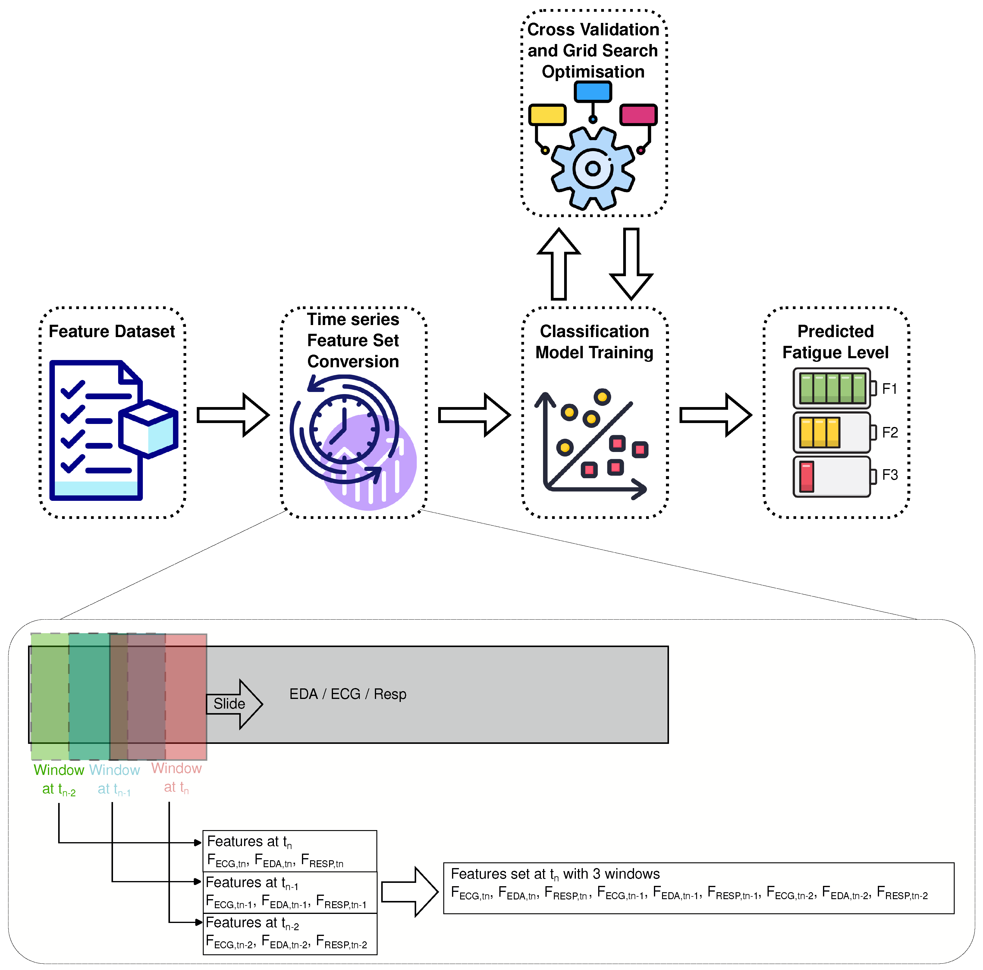
• The ML models used to capture time-related variations associated with mental fatigue often rely on complex models, such as RNN and LSTM. While these models excel in learning feature characteristics and their temporal variability, integrating them into real-time applications using wearable devices with limited processing capacity is challenging. To address this constraint, we employ a feature sequencing and set compression technique to prepare time-series “like” data for presentation to ML algorithms that are not specialized in processing sequential data. We demonstrate that this technique enhances the model accuracy. Notably, our model was used to detect mental fatigue using physiological signals from [30] and achieved a maximum accuracy of 98%.

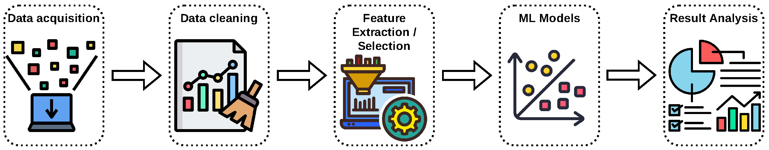
3. Materials and Methods

The conventional ML pipeline was followed in our methodology, as depicted in Figure 1, but with a particular emphasis given to feature extraction and selection techniques. First, the collected data were cleaned, to eliminate unwanted noise and artifacts. Then, the clean data were processed to extract and select features. This step was crucial in our study: as previously mentioned, selecting appropriate features is important for constructing accurate and, most importantly, relevant ML classification models, which will be developed in the subsequent step. Finally, we evaluated the ML models and compared their performance.

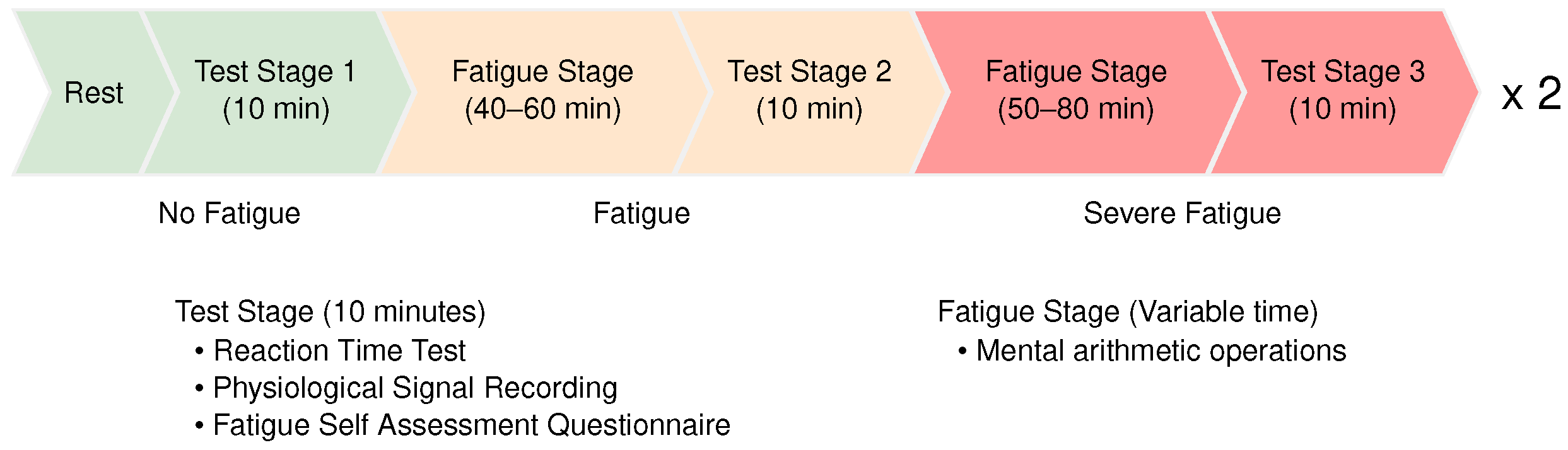
3.1. Data Description

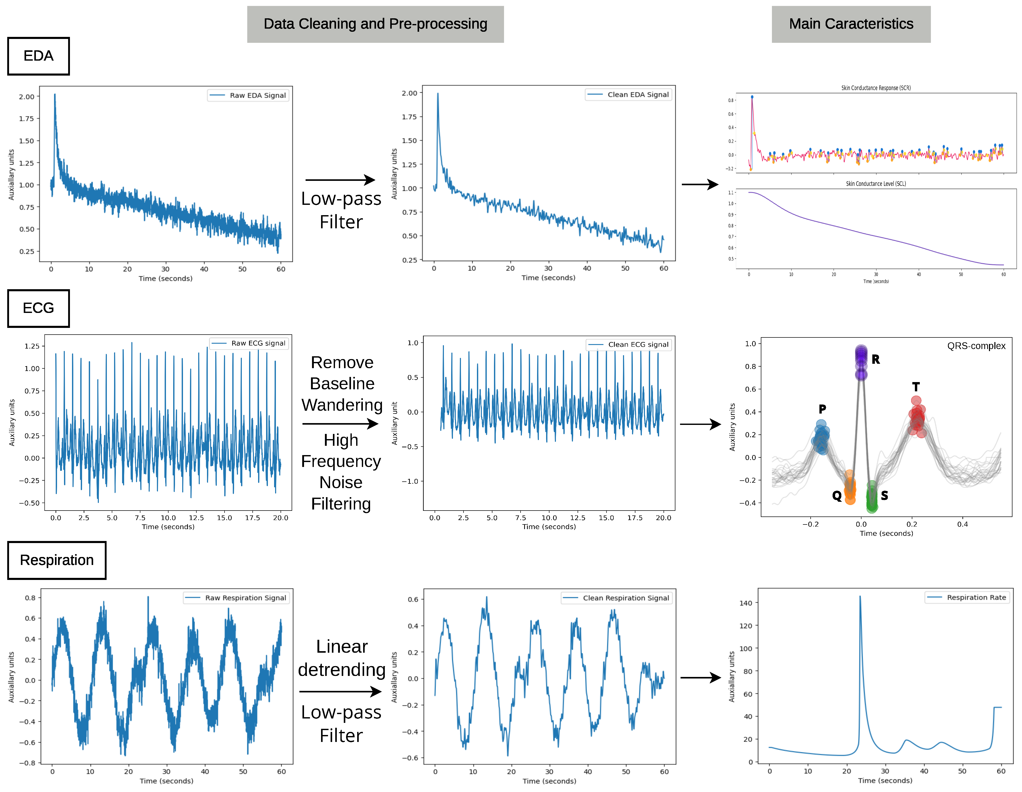
The data utilized in this study were obtained by request from the original owners, Zeng et al. in [30]. As a result, the data description provided in this paragraph is based on the limited information available in [30], supplemented by insights deduced from the raw data and the details provided by Zeng et al. via email. These data represent a collection of physiological signals, including ECG, EDA, and respiration signals. The data acquisition involved three healthy subjects, each engaged in a sequence of mental tasks (cf. Figure 2). These tasks encompassed a structured progression, commencing with a rest stage, followed by successive stages of fatigue assessment (test stage) and fatigue induction (fatigue stage). For the purpose of this study, we categorized the data from the test stages into three distinct levels: no fatigue, fatigue, and severe fatigue, as previously performed in [30]. The mental task initiation involved an initial rest period, to ensure that the subjects began in a non-fatigue state. Subsequently, the subjects underwent the first test stage, during which their mental fatigue level was assessed based on an objective measure and a subjective measure, alongside concurrent recording of physiological signals, spanning a duration of 10 min. The objective measure was based on a reaction-time test, where the subjects had to react to a stimulus as quickly as possible. The subjective measure was based on a questionnaire, where the subjects described their feeling of fatigue on a scale of 0 to 9. The subjects underwent the first fatigue stage, where they engaged in intense mental work until they felt tired and sleepy. Then, they were subject to a second test stage in the same manner as the first test stage. Similarly, in the second fatigue stage, they performed an intense mental task until they felt exhausted. Finally, they performed the third test stage. The entire process was repeated, resulting in 60 min of data for each subject. To label the data, the fatigue levels were determined through a combined analysis of subjective questionnaires and objective measures from the test stages. The subjective scores were ≤3 for no fatigue, ≥3 and <6 for fatigue, and ≥6 for severe fatigue. The objective measures, i.e., reaction-time tests, had a similar upward trend and the average reaction times increased from 461 ms in the no fatigue stage to 501 ms in the fatigue stage and then to 736 ms in the severe fatigue stage.

Table 1. Physiological data summary.

Signal	Sampling Interval (ms)	Sampling Frequency (Hz)	Full Length of the Analysed Signal
ECG	5	200	120,000
EDA	100	10	6000
Respiration	120	8.33	5000

and Figure 3 summarize the characteristics of the physiological signals obtained during the test stages. In Figure 3, the range of amplitudes in each signal is represented by the respective box plots, with the bottom and top edges of the box indicating the 25th and 75th percentiles of the amplitudes, the whiskers showing the extreme amplitude points, the mean value highlighted by the dashed red line, and the median value highlighted by the purple line. Note that the data from the first test stage 1 for one of the subjects were corrupted. Therefore, there are 5 records of 10 min for one subject and 6 records of 10 min for the other two, accounting for a total of 170 min of physiological signals.

3.2. Data Cleaning

For the data cleaning process, we employed NeuroKit2 [31], an open-source Python package designed for processing neuro-physiological signals. The cleaning process for each signal is described in the following paragraphs.

3.2.1. Electrodermal Activity (EDA)

In this study, the EDA signal was cleaned through noise removal and signal smoothing. To achieve this, a low-pass filter with a 3 Hz cut-off frequency and a 4th order Butterworth filter were applied, as shown in the top row of Figure 4. Additionally, low-frequency artifacts, likely caused by deformation of the sensor-skin interface, in the EDA data were manually eliminated. Subsequently, the EDA data were decomposed into SCL and SCR data series using the Biopac Acqknowledge algorithm [32]. In this process, the raw EDA data underwent median value smoothing, and the filtered waveform was then subtracted from the original data. Since the median value smoothing discards areas of rapid change, subtracting the smoothed waveform leaves behind only the sections of rapidly changing SCR data. On the other hand, SCL data were obtained by passing the raw EDA data through a low-pass filter with a cut-off frequency of 0.05 Hz.

3.2.2. Electrocardiogram (ECG)

The ECG signal was filtered and processed, to detect individual heart beats (see middle row of Figure 4). The first step was to remove baseline wandering. For that purpose, a 4th order Butterworth high-pass filter with a cut-off frequency of 0.5 Hz was used. More precisely, the filter transfer function of order 2 was used, but the filtering was performed in forward and reverse directions, creating a zero-phase filtered signal and a resulting order of four [33]. It is worth mentioning that such filtering is typically preferred when it is feasible, to have access to the entire input signal in advance. However, in real-time processing scenarios, this may introduce some delay. Despite this inconvenience, we opted for bi-directional filtering, because it offered superior noise reduction and a more effective frequency response for the given data, which was essential for artifact elimination. In a general context, this approach can be substituted with unidirectional (causal) filtering, as discussed in [34]. The high-frequency power line noise was filtered by smoothing the signal with a moving average kernel with a width of one period of 50 Hz. Then, the Pan–Tompkins method [35] was used to detect the QRS complex and, eventually, R-peaks from the filtered ECG signal. Finally, the time intervals between each two consecutive R-peaks were sequenced to determine the heart rate variability (HRV). A fast Fourier transform (FFT) was used to obtain the power spectral density (PSD) of the HRV.

3.2.3. Respiration

The respiration signal was filtered to remove baseline drift and high-frequency noise. The slow baseline drifts and fluctuations in the signal were removed by applying a high-pass filter at 0.05 Hz. The high-frequency noise was filtered by applying a low-pass filter at 3 Hz. Then, the signal was processed using a zero-crossing algorithm [36] to detect the breathing cycle (see bottom row of Figure 4).

3.3. Feature Engineering

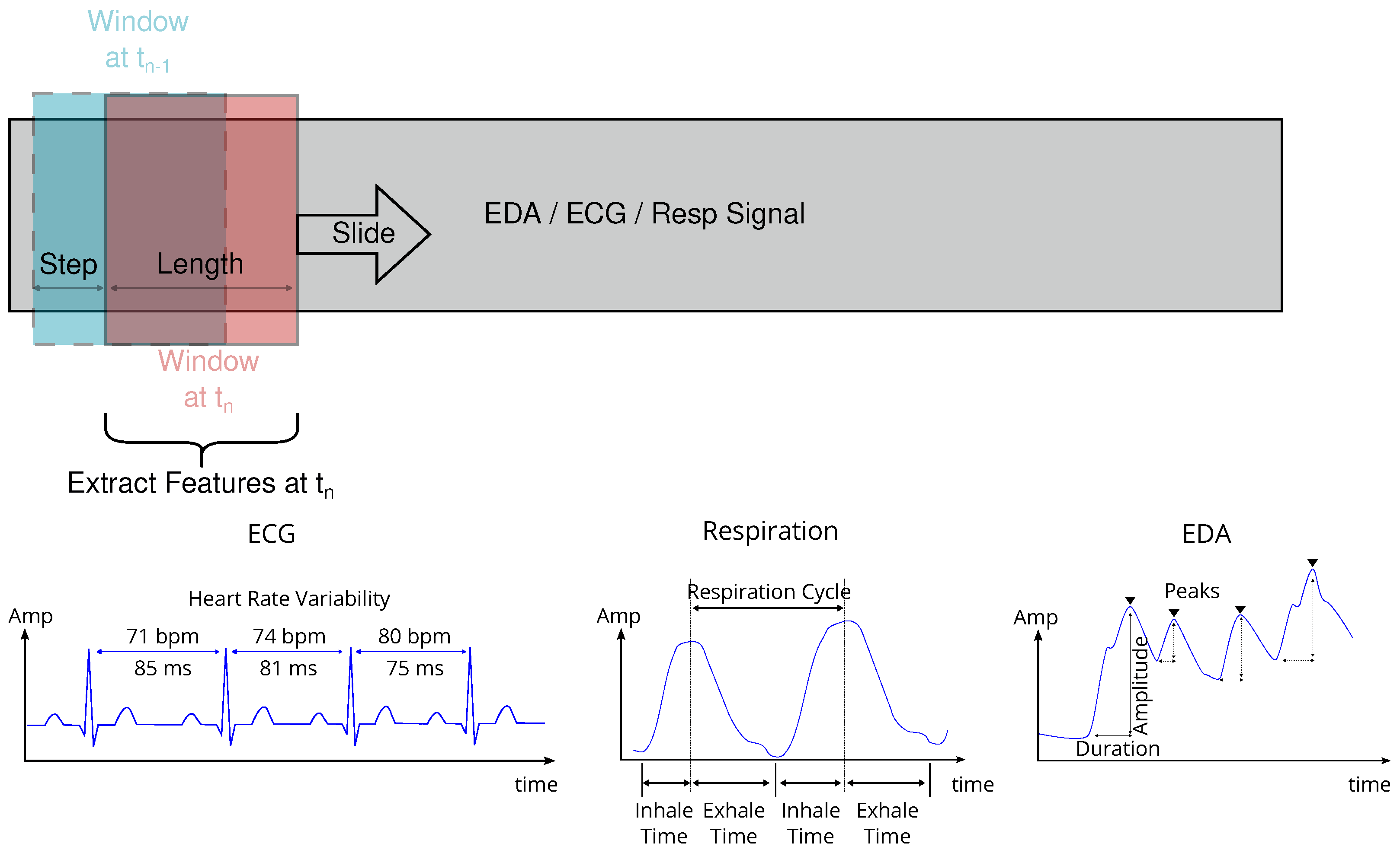
3.3.1. Windowing

An overview of the feature extraction process is shown in Figure 5. One basic design question is the extraction of static features from temporal signals. Indeed, the characteristics of physiological signals can be of variable length; for instance, the QRS-complex in an ECG signal is used to extract heart rate features, and the duration of each QRS-complex and intervals between consecutive QRS-complexes are of variable nature; similarly, the SCR component of the EDA signal varies with stimuli. Thus, we used a sliding window of fixed length on each physiological signal to extract features. This allowed analyzing the signals over smaller segments, making it easier to capture temporal patterns and variations in the data while extracting features. The key issue is to choose the right length and step size for the sliding window. If a short-time portion of a signal is processed, it may not contain sufficient information to identify features, whereas a longer-time portion of the signal is not suitable for real-time applications, due to a longer processing time. A correct step size for “sliding” the window is essential to maximize the capture of useful information, while eliminating redundancy and edge effects.

Based on the experimental observations (discussed later in Section 5), we found a window length of 60 s and a step size of 3 s to be the best choice for the given physiological signals. Therefore, this is used to illustrate the feature extraction and feature selection processes discussed in the following paragraphs.

3.3.2. Feature Extraction

Table 2. List of features extracted from the EDA, ECG, and respiration signals, using a sliding window of length 60 s and step size of 3 s.

Signal	Feature	Description	Var.	Corr. f.stage	Sel
EDA	SCR.peak.rate	Number of SCR peaks.	0.042	0.31
	SCR.amp.sum	Sum of SCR peak amplitudes.	0.019	0.15
	SCR.dur.sum	Sum of SCR peak durations.	0.033	0.26
	SCR.mean.amp	Mean amplitude of SCR peaks.	0.037	0.26	✓
	SCR.mean.dur	Mean duration of SCR peaks.	0.0085	0.24	✓
	mean.SCL	Mean value of tonic activity.	0.029	0.14
	SCL.SD	Standard deviation of tonic     activity.	0.027	0.1
ECG	mHR	Mean heart rate.	0.041	0.17	✓
	HRV.MeanNN	Mean of the RR intervals.	0.044	0.18	✓
	HRV.SDNN	Standard deviation of the RR      intervals.	0.038	0.1	✓
	HRV.VLF	Very low frequency (0.0033–0.04 Hz) spectral power.	0	0
	HRV.LF	Low frequency (0.04–0.15 Hz)      spectral power.	0.060	0.09
	HRV.HF	High frequency (0.15–0.4 Hz)      spectral power.	0.046	0.12
	HRV.VHF	Very high-frequency (0.4–0.5 Hz) spectral power.	0.025	0.11
	HRV.LFHF	Ratio of low-frequency power to high-frequency power.	0.018	0.12
Respiration	RSP.rate	Mean breathing rate.	0.038	0.31	✓

Var.: variance. Corr. f.stage: correlation of feature with respect to the fatigue stages.

summarises the series of features extracted from the EDA, ECG, and respiration signal.

As for EDA, the SCR component was used to identify SCR peaks and compute the sum of peak amplitudes, sum of peak durations, number of peaks, mean peak amplitude, and mean peak duration. Note that, the SCR with an amplitude over a specified threshold (the commonly used threshold is 0.03 $\mathsf{\mu }$S) was regarded as a significant SCR. The SCL component was used to compute the mean value and standard deviation of the SCL amplitude.

For ECG, the most commonly used features in the time domain and frequency domain were extracted. In the time domain, the mean heart rate in beats per minute and the HRV were the most prominent. The main method used to quantify HRV was to measure the amount of variance in inter-beat intervals: the time intervals between successive RR peaks. HRV-based features included the mean RR peak interval, and standard deviation of the RR interval. The frequency-domain measures, categorized as very low-frequency, low-frequency, high-frequency, very high-frequency, and ratio of low frequency to high-frequency, reflect the distribution of the spectral power of the HRV across different frequencies bands, as the different regulatory systems modulate the heart rate at distinct frequencies. The respiration rate was extracted from the respiration signal, not only as a feature, but also to eliminate potential artifacts from ECG data.

3.3.3. Features Selection

To train an optimal and relevant ML model, we needed to make sure that we used only the essential features. The feature selection was performed in two steps: numerical analysis and contextual analysis.

In the numerical analysis, first, a variance analysis was performed on all features (cf. Table 2). To prevent bias, all the features were normalized between their maximum and minimum values. Then the variance threshold approach was used to removes all features whose variance was inferior to a threshold. By default, this removes all zero-variance features, i.e., features with the same value in all samples. We arbitrarily considered a threshold of 0.03 to remove features with very little variance. We assumed that features with a higher variance may have contained more useful information. Note that this method did not take the relationship between the feature and target variable (in our study, fatigue level) into account. Thus, it was combined with a correlation analysis using the Pearson correlation coefficient. Therefore, only the features with a low correlation coefficient and low variance were eliminated.

Note that the above method of feature selection is purely mathematical, it does not take into account the contextual information of the study. This is a common problem found in the literature and that impacts the modeling process, notably in the context of fatigue detection systems. Such an issue is also pointed out in [37]. Indeed, the physiological signals can be easily influenced by the experiment design used to collect data and assess fatigue, particularly the EDA signal. As mentioned earlier, the phasic component or SCR provide moment-to-moment arousal measurement, reflecting responses specific to stimuli. This is because SCR is composed of two sub-components: event-related SCR, which occurs following specific stimuli, and non-specific SCR, which often occurs due to internal cognitive events. We recall that the data used in this study were collected during a response-time test, where the subject had to respond to each stimulus as quickly as possible. Moreover, the stimuli were presented at random time intervals. In this context, the features like SCR.peak.rate, SCR.amplitude.sum, and SCR.duration.sum entirely depend on the number of stimuli present/absent in a given time window, but not on the fatigue state, due to their dependence on the number of peaks in this time window. Consequently, we rejected these features, despite their high variance and correlation. On the contrary, we proposed using SCR.mean.amplitude and SCR.mean.duration, which less affected by the number of peaks and more by the characteristics of these peaks.

For ECG, we selected only the time domain features, since the frequency domain features required a long window length (≥120 s) to represent any significant information.

Before moving to the modeling phase, the quality of these features was assessed through a statistical null hypothesis validation. This allowed us to test for a statistically significant difference in feature values among the three fatigue states. For this purpose, we employed a Kruskal–Wallis test. This is a commonly used statistical test to compare two or more groups of non-normal continuous data, which was the case for our dataset.The Kruskal–Wallis test results in a low p-value when the compared group of data are significantly different from one another. In our test, the feature values from all the subjects were grouped to create three groups based on their respective fatigue states. The results revealed a statistically significant difference with $p<0.05$ for all the features between the three fatigue states, as summarized in

Table 3. Kruskal–Wallis null hypothesis test used on the selected features in the three fatigue states.

Feature	Score	p
SCR.mean.amp	67.30	$0.024\times {10}^{-13}$
SCR.mean.dur	73.16	$0.012\times {10}^{-14}$
mHR	14.43	$0.073\times {10}^{-2}$
HRV.MeanNN	14.86	$0.059\times {10}^{-2}$
HRV.SDNN	83.39	$0.077\times {10}^{-17}$
RSP.rate	120.99	$0.053\times {10}^{-25}$

.

4. Modeling

Figure 6 illustrates our ML modeling process. The sliding window employed in the previous step to obtain the features dataset allows capturing the variation and temporal patterns in the features. These features can be used to train ML algorithms for classification. Our objective was to predict one of the three fatigue levels in real-time applications. For that purpose, we opted for the random forest (RF) algorithm [38], which combines predictions from multiple decision trees and offers several advantages. For instance, it mitigates the risk of overfitting and enhances the model’s generalization ability, and it excels at capturing non-linear relationships, which is important for modeling the complex, potentially non-linear connections between physiological signals and the cognitive fatigue level. Additionally, it can achieve relatively better results with less input data as compared to advanced algorithms based on neural networks, which are data-greedy.

However, the RF algorithm is not inherently designed to handle the temporal dependencies and sequential patterns present in time-series data. Thus, a feature decomposition and set conversion technique was introduced. This involved converting the sequential features extracted from the sliding window into a single set of values, which were then used for training the classification model. This process does not impact the class of the signal, as it is performed on the data from each fatigue state separately. This meant the original class annotations (no fatigue, fatigue, and severe fatigue) were preserved.

For evaluation purposes, we compared the RF algorithm with multiple ML algorithms [38] including support vector machines (SVM), k-nearest neighbors (KNN), decision trees (DT), and gradient boosting (GB). The results revealed that the RF algorithm achieved the highest accuracy in classifying fatigue states. In each comparison scenario, during the model training phase, hyperparameter tuning using the grid search algorithm and cross-validation using K-folds were applied, to achieve the best accuracy, while mitigating overfitting issues. Finally, the trained classifier performance was evaluated based on two widely used performance metrics, namely accuracy and F1 score. A visual representation of the model performance is given by ROC curves.

The accuracy and F1 score are given by the following equations:

$$acc=\frac{TP+TN}{TP+TN+FP+FN}$$

$$F1=\frac{2\times TP}{2\times TP+FP+FN}$$

where TP represents true-positive predictions (i.e., correctly predicted as correct), TN corresponds to true-negative predictions (i.e., correctly predicted as incorrect), FP represents false-positive predictions, and FN represents false-negative predictions.

Note that these formulas give an accuracy and F1 score for each output class separately. Since our study involved classification into three output classes (no fatigue, fatigue, and severe fatigue), we present the results in terms of the average accuracy and macro-averaged F1 score, to evaluate the overall performance of the models. These were obtained using the following equations:

$$\mathit{averaged\; accuracy}=\frac{\mathit{sum}\mathit{of}\mathit{accuracy}\mathit{per}\mathit{class}}{3}$$

$$\mathit{macro\; averaged\; F}\mathit{1} \mathit{score}=\frac{\mathit{sum}\mathit{of} \mathit{F}\mathit{1}\mathit{scores}\mathit{per}\mathit{class}}{3}$$

5. Results and Discussion

In this section, we evaluate our modeling process and the resulting RF-based ML classification model under different constraints. In each scenario, a feature dataset from all subjects and all fatigue stages was combined. It contained 1086 values per feature and per fatigue stage. This combined dataset was randomly split into training with validation (80%) and testing (20%) subsets.

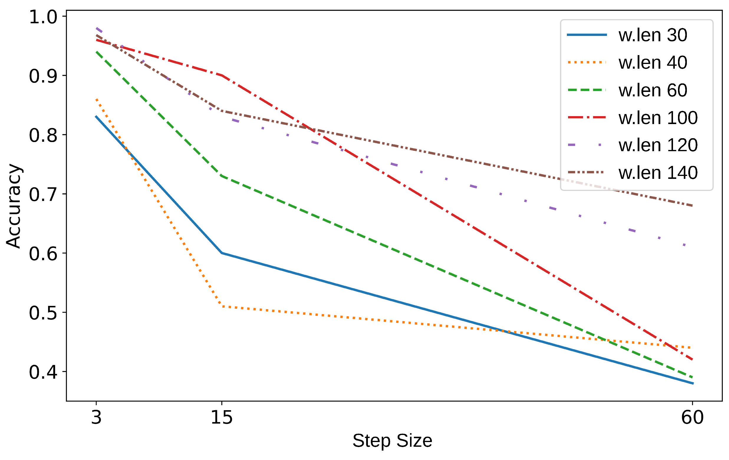
5.1. Windowing Analysis

Let us start by analyzing the impact of window length and step size on the model’s classification accuracy. For that purpose, we varied the window length from 30 s to 140 s and the step size from 3 s to 60 s, as shown in Figure 7. Each curve in Figure 7 corresponds to a fixed window length. The x-axis represents an increasing step size, while the corresponding accuracy for each step size is shown on the y-axis. In each case, a similar pattern was observed: the classification accuracy increased with longer window lengths and decreased with larger step sizes. This trend can be explained as follows: a shorter window step results in more overlap between adjacent windows, mitigating information loss (potentially due to edge effects) and capturing more temporal patterns, whereas a longer window captures more information from each input physiological signal and the extracted features tend to be more stable and less susceptible to noise or short-term fluctuations. However, longer windows introduce a delay in the system’s response. From a real-time application point of view, where a smaller window size can be preferred, we consider that a window with a length of 60 s and a step size of 3 s provides a good trade-off between accuracy and response time; thus, this was used in the remainder of the model performance evaluation.

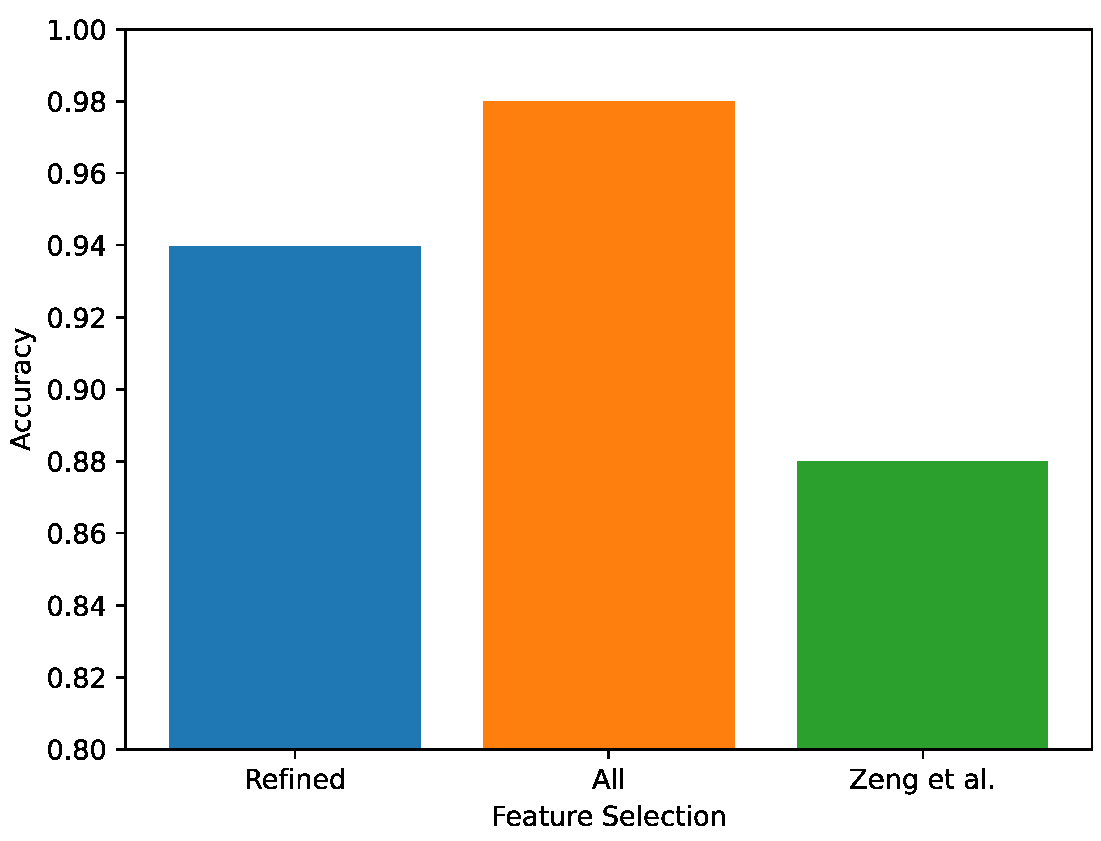
5.2. Feature Selection Analysis

The feature selection approach used in our study (cf. Section 3.3.3) incorporated both numerical and contextual analysis. The primary objective of this approach is to select features that are relevant to the given experiment design. We assessed the selected features by analyzing the model performance in terms of accuracy in classifying the fatigue states. Furthermore, we show that a method that does not follow a careful feature selection process can yield misleading results. For that purpose, we compared RF-based models trained on three sets of features from Table 2:

• Refined features (our selected features): SCR.mean.amp, SCR.mean.dur, mHR, HRV.-MeanNN, HRV.SDNN, and RSP.rate;
• Zeng et al.’s features (i.e., the features used in [30]): SCR.peak.rate, SCR.amp.sum, SCR.dur.sum, mHR, HRV.SDNN, and RSP.rate;
• All features from Table 2: the commonly used features in the literature, including our selected features and those of Zeng et al.

The results are presented in Figure 8, where our selected features led to a classification accuracy of 94%.

The features of Zeng et al. gave an accuracy of 88%. However, as mentioned in Section 3.3.3, the value of the EDA features SCR.peak.rate, SCR.amp.sum and SCR.dur.sum is highly dependent on the number of peaks, which depend on the number of stimuli present in a given time window during the feature extraction, rather than the fatigue state. Recall that the data used in this study were obtained by Zeng et al. in [30] during a reaction time test, in which stimuli were presented at random time intervals. Since the precise timing of these stimuli is not known, the model trained using the features of Zeng et al., despite achieving an accuracy of 88%, provides an irrelevant output for fatigue detection.

A common technique used in the literature to achieve high accuracy is to increase the number of features in model training. For instance, the model trained with all the features from Table 2 achieved the highest accuracy of 98%. However, these features also included the incorrect features of Zeng et al. Additionally, they included ECG frequency domain features (HRV.VLF, HRV.LF, HRV.HF, HRV.VHF, and HRV.LFHF), which may not represent any meaningful information about the cognitive state when a small time window of 60 s is considered [39,40]. Thus, the models output, despite an accuracy of 98%, may be misleading. As previously explained in Section 3.3.3, our selected features did not encounter the same issues as those of Zeng et al. and were more aligned with the requirements of the experiment based on a reaction time test. Additionally, they resulted in a classification accuracy of 94%.

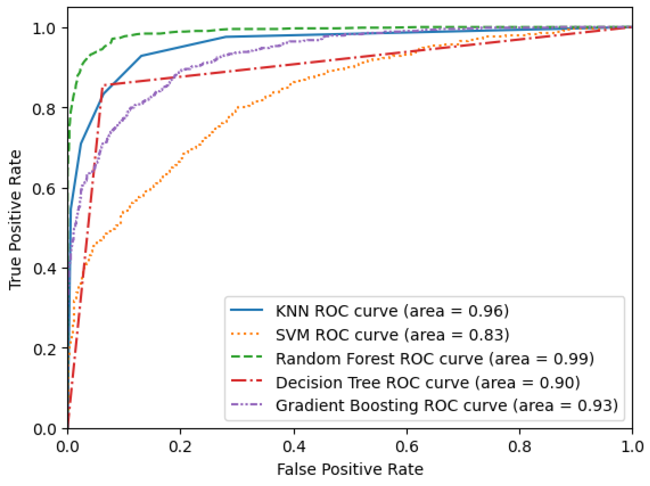
5.3. Classification Algorithm Analysis

The RF-algorithm-based model was compared to other algorithms with similar complexities, namely SVM, KNN, DT, and GB. The comparison results are summarized in

Table 4. Average accuracy and macro averaged F1-score of the different classification models with and without the time-series feature set.

Model	Accuracy without TS Feature Set Conversion	F1-Score without TS Feature Set Conversion	Accuracy with 2 Windows	F1-Score with 2 Windows	Accuracy with 3 Windows	F1-Score with 3 Windows	Accuracy with 5 Windows	F1-Score with 5 Windows
SVM	0.66	0.66	0.64	0.64	0.65	0.64	0.7	0.7
KNN	0.87	0.87	0.85	0.85	0.85	0.85	0.88	0.88
DT	0.85	0.85	0.83	0.83	0.81	0.81	0.8	0.8
GB	0.83	0.84	0.82	0.83	0.8	0.8	0.82	0.82
RF	0.94	0.94	0.96	0.96	0.96	0.96	0.98	0.98

and Figure 9.

For comparison, two different cases were considered. In the first case, the models were trained without a time-series feature set conversion technique, i.e., the features extracted at each window step were sequentially presented as input to train the model. In this case, the maximum accuracy of 94% and F1-score of 94% was achieved by the RF algorithm, while KNN, DT, GB, and KNN achieved relatively low accuracies and F1-scores.

In the second case, the models were trained with input feature sets obtained from time-series feature set conversion (cf. Section 4). In Table 4, the results obtained using the feature sets from 2, 3, and 5 consecutive windows are presented. The results were unchanged when more than five window steps were considered, and these are not presented. The results indicated that the performance generally improved with an increasing number of windows for the SVM, KNN, and RF models. In each case, the RF algorithm consistently achieved the highest accuracy and F1 score. The best performance observed was an accuracy and F1-score of 98% when five windows were considered. The SVM algorithm shows the worst performance in all cases.

A graphical analysis of the results is presented using ROC curves in Figure 9. A ROC curve is constructed by plotting the true positive rate (TPR) against the false positive rate (FPR). TPR is the proportion of observations that were correctly predicted to be positive out of all positive observations (TP/(TP + FN)). Similarly, the FPR is the proportion of observations that were incorrectly predicted to be positive out of all negative observations (FP/(TN + FP)). Thus, the ROC curve shows the trade-off between sensitivity (or TPR) and specificity (1 − FPR). Classifiers that give curves closer to the top-left corner indicate a better performance. As a baseline, a random classifier is expected to give points lying along the diagonal (FPR = TPR). The closer the curve comes to the 45-degree diagonal of the ROC space, the less accurate the classifier.

In order to apply the ROC for multiclass classification (in our case three fatigue states), the notion of a one-vs-rest ROC curve was used and micro averaging was performed to summarize the information of the multiclass ROC curves. A one-vs-rest ROC curve consisted in computing a ROC curve for each of the three classes. In each step, a given class was regarded as the positive class and the remaining classes were regarded as the negative class as a bulk. Micro-averaging aggregated the contributions from all the classes to compute the average metrics, as follows:

$$TPR=\frac{{\sum }_{class}T{P}_{class}}{{\sum }_{class}(T{P}_{class}+F{N}_{class})},FPR=\frac{{\sum }_{class}F{P}_{class}}{{\sum }_{class}(F{P}_{class}+T{N}_{class})},$$

Figure 9 shows that the RF classifier had a greater discriminative capacity and higher performance, since it approaches farther to the top-left corner compared to others. For comparison, it can be useful to summarize the performance of each classifier into a single measure. One common approach is to calculate the area under the ROC curve (AUC). This is equivalent to the probability that a randomly chosen positive instance is ranked higher than a randomly chosen negative instance. The ideal ROC curve thus has an AUC = 1.0 and as a general rule, for any classifier output to be meaningful the AUC must be greater than 0.5, and it must be greater than 0.8 to be considered acceptable. The ROC curve with the largest AUC is considered to have a better performance. In our results, the RF classifier showed the highest AUC of 0.99, KNN had an AUC of 0.96, which was greater than that of GB (0.93), and DT had 0.90. In contrast, SVM exhibited the lowest AUC of 0.83.

When the time-series feature set conversion is considered, the enhancement of the RF model performance is also visible in the ROC curve in Figure 10 as the number of windows was increased from 1 to 5. The AUC was 0.99 in all the cases.

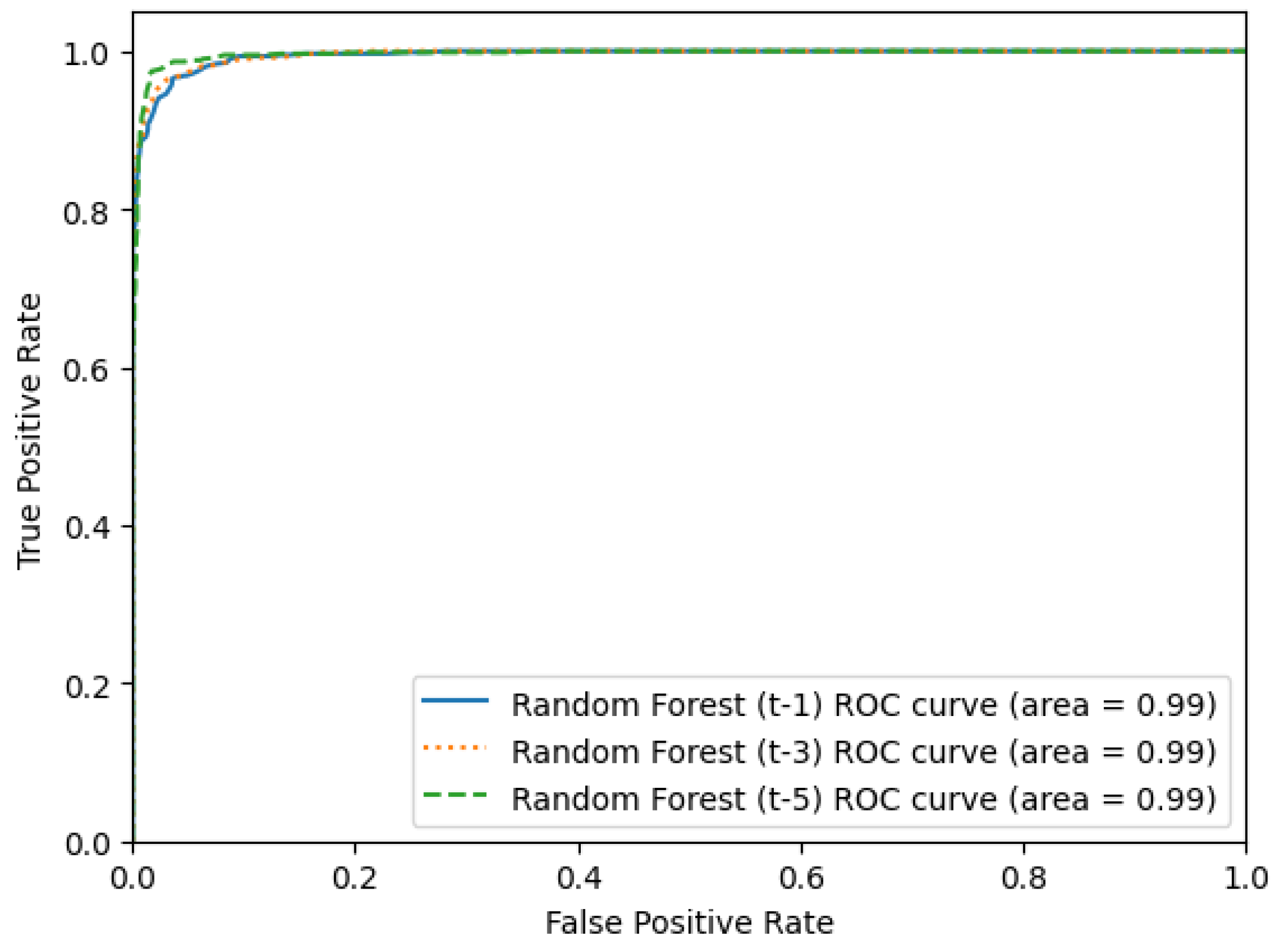
5.4. Cross-Validation Analysis

To assess the reliability of the model performance, K-fold cross-validation was applied on the best RF-based model obtained in the previous steps. This technique allowed estimating how well the model would performed on unseen data or data it was not trained on. For that purpose, five-fold cross-validation was employed, which means the model was trained and evaluated five times. The combined dataset from all the subjects and fatigue stages was randomly split into five subsets (called folds), with each fold serving as the testing set once, while the remaining folds were used for training. For each test fold, the obtained accuracy and F1-score are summarized in

Table 5. K-fold analysis of the RF model.

K-Fold	Accuracy	F1-Score
1	0.98	0.98
2	0.95	0.95
3	0.96	0.96
4	0.96	0.96
5	0.95	0.95
Average	0.96	0.96

. The results indicate very little variability, with the accuracy and F1-score varying between 0.95 and 0.98. This suggests that the model’s output was relatively stable and less sensitive to specific data splits. Therefore, an average performance of 0.96 can be expected on new, unseen data.

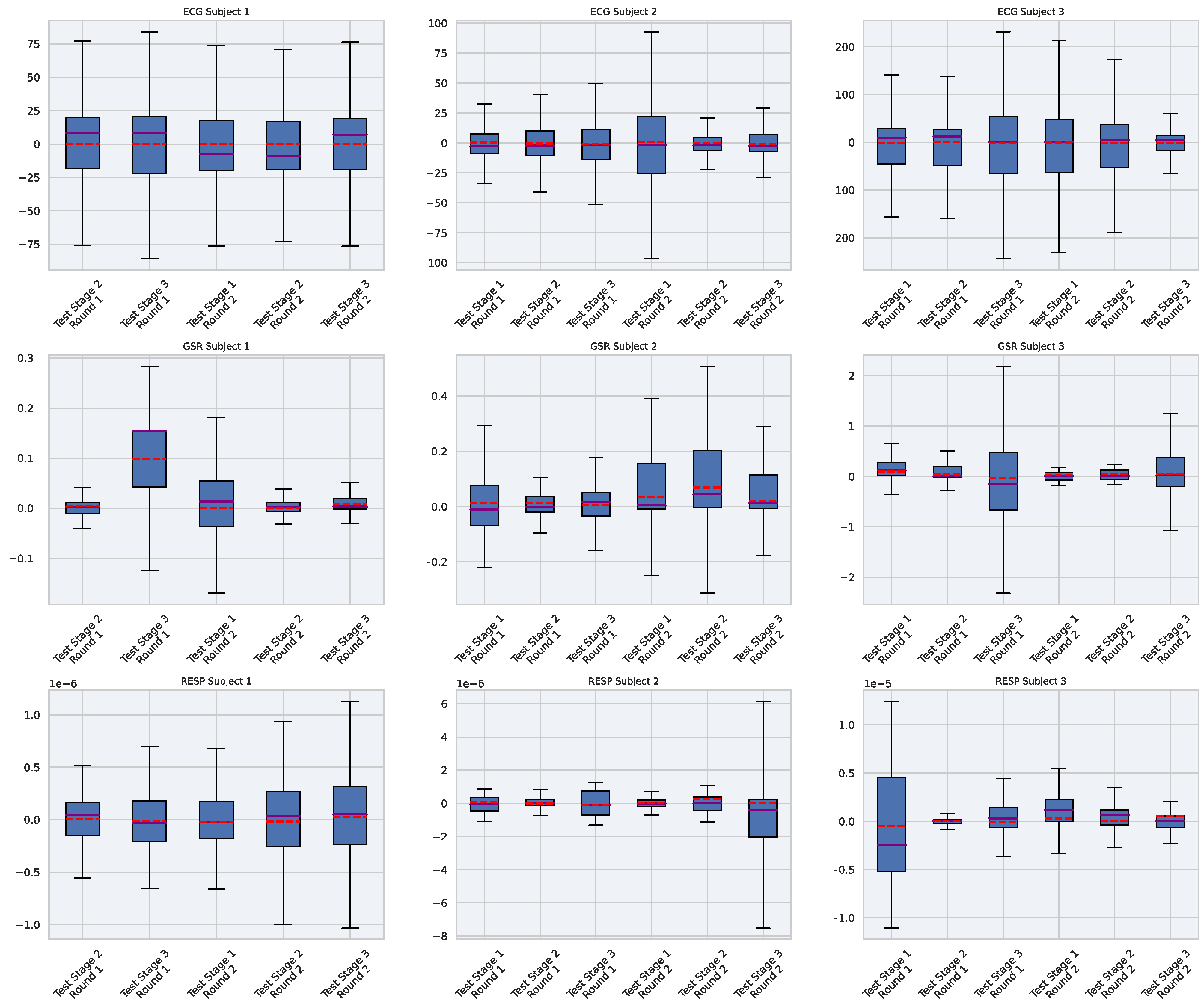
5.5. Per Subject Variability Analysis

The random split used in the cross-validation analysis did not allow independent testing for the given three subjects. Therefore, to observe the model performance variability per subject, separate tests were performed, in which the RF model was trained on data from two subjects and tested on the remaining subject. However, this type of analysis for the classification of fatigue states can be affected by the well-known problem of inter-individual variability [41]. Indeed, mental fatigue and its markers vary among individual subjects. An ML model trained on one set of subjects and tested on another subject cannot capture this variability in fatigue-related features. This problem can be reduced by retraining the same ML model on a small subset of the data from the subject to be tested.

Table 6. Per subject analysis of the RF model.

Train	Re-Train	Test	Accuracy on Test without Re-Training	F1-Score on Test without Re-Training	Accuracy on Test (80%) with Re-Training (20%)	F1-Score on Test (80%) with Re-Training (20%)
Subject 1 and 2	Subject 3	Subject 3	0.68	0.68	0.88	0.88
Subject 2 and 3	Subject 1	Subject 1	0.7	0.69	0.93	0.93
Subject 3 and 1	Subject 2	Subject 2	0.7	0.6	0.88	0.88

shows the RF model performance results under two settings. In the first, the model was trained on data from only two subjects and tested on the remaining subject. This resulted in a test accuracy of 68% for subject 3 and 70% for subjects 1 and 2. In the second case, the corresponding models were retrained on a data subset (20% of the full data size), and they were tested on the remaining data subset (80%) of the subject to be tested. In this case, five-fold cross-validation was used to obtain the mean performance. This resulted in an increased model accuracy of 88% for subjects 3 and 2 and 93% for subject 1. Nevertheless, we cannot prove that our model can be generalized to new participants whose data have never been used to train the model. Inter-individual variability (sensitivity to drowsiness and physiological/behavioral/psychological peculiarities) can be a limiting factor for generalization (i.e., the model’s behavior with previously unseen data). Achieving near-generalization behavior would require multiple replications of the experiment and studies conducted under the same conditions over a longer period.

6. Conclusions and Perspective

This research presents a machine learning modeling process for detecting mental fatigue using physiological signals, including EDA, ECG, and respiration signals as markers of fatigue. We implemented a RF-based model to classify three levels of fatigue. This model was compared to SVM-, KNN-, DT-, and GB-based models.

In contrast to traditional modeling practices that aim to increase the number of features, we demonstrated that careful feature selection can lead to high model performance, while ensuring reliability and reducing the number of features. We identified EDA features (SCR mean amplitude and SCR mean duration), ECG features (mean heart rate and HRV standard deviation), and respiration rate as highly relevant in detecting mental fatigue when the reaction time test was used in the experiment design.

The main objective of our study was to emphasize the importance of the feature selection process, taking into account the details of experiment design and highlighting the common problem whereby the literature can lead to misleading results.Our study was limited to the analysis of a small dataset, obtained from the research published in [30]. To further validate the selected features and observe their variation with respect to the subject profiles, such as age, gender, health etc, a study on a larger dataset would be required.

Furthermore, we employed a sliding-window-based feature extraction and feature set conversion technique to train the RF model, incorporating the temporal aspect of physiological signals. A thorough evaluation of our model resulted in an average an accuracy and F1-score of 96%. In the current study, we considered a uniform length of window for all the features, to ensure timely output and simplicity. However, the different signals (ECG, EDA, and respiration) and their derived features have different frequencies and variabilities over time. In our future work, we will explore the optimal window length and step size for individual signals.

References

1. Wang, Q.; Yang, J.; Ren, M.; Zheng, Y. Driver Fatigue Detection: A Survey. In Proceedings of the 2006 6th World Congress on Intelligent Control and Automation, Dalian, China, 21–23 June 2006; Volume 2, pp. 8587–8591. [Google Scholar] [CrossRef]
2. Wang, X.; Xu, C. Driver drowsiness detection based on non-intrusive metrics considering individual specifics. Accid. Anal. Prev. 2016, 95, 350–357. [Google Scholar] [CrossRef] [PubMed]
3. Brown, I.D. Driver Fatigue. Hum. Factors 1994, 36, 298–314. [Google Scholar] [CrossRef] [PubMed]
4. Brookhuis, K.A.; de Waard, D. Monitoring drivers’ mental workload in driving simulators using physiological measures. Accid. Anal. Prev. 2010, 42, 898–903. [Google Scholar] [CrossRef]
5. Dingus, T.A. Development of Models for Detection of Automobile Driver Impairment. Ph.D. Thesis, Faculty of Virginia Polytechnic Institute, Blacksburg, VA, USA, 1985. [Google Scholar]
6. Thiffault, P.; Bergeron, J. Monotony of Road Environment and Driver Fatigue: A Simulator Study. Accid. Anal. Prev. 2003, 35, 381–391. [Google Scholar] [CrossRef] [PubMed]
7. Weng, C.H.; Lai, Y.H.; Lai, S.H. Driver Drowsiness Detection via a Hierarchical Temporal Deep Belief Network. In Proceedings of the Computer Vision—ACCV 2016 Workshops, Taipei, Taiwan, 20–24 November 2016; Chen, C.S., Lu, J., Ma, K.K., Eds.; Lecture Notes in Computer Science. Springer: Cham, Switzerland, 2017; pp. 117–133. [Google Scholar] [CrossRef]
8. Benzo, R.M.; Farag, A.; Whitaker, K.M.; Xiao, Q.; Carr, L.J. Examining the Impact of 12-Hour Day and Night Shifts on Nurses’ Fatigue: A Prospective Cohort Study. Int. J. Nurs. Stud. Adv. 2022, 4, 100076. [Google Scholar] [CrossRef]
9. Givi, Z.; Jaber, M.; Neumann, W. Modelling Worker Reliability with Learning and Fatigue. Appl. Math. Model. 2015, 39, 5186–5199. [Google Scholar] [CrossRef]
10. Bentall, R.P.; Wood, G.C.; Marrinan, T.; Deans, C.; Edwards, R.H.T. A Brief Mental Fatigue Questionnaire. Br. J. Clin. Psychol. 1993, 32, 375–377. [Google Scholar] [CrossRef]
11. Shahid, A.; Wilkinson, K.; Marcu, S.; Shapiro, C.M. Visual Analogue Scale to Evaluate Fatigue Severity (VAS-F). In STOP, THAT and One Hundred Other Sleep Scales; Shahid, A., Wilkinson, K., Marcu, S., Shapiro, C.M., Eds.; Springer: New York, NY, USA, 2011; pp. 399–402. [Google Scholar] [CrossRef]
12. Lee, I.S.; Bardwell, W.A.; Ancoli-Israel, S.; Dimsdale, J.E. Number of Lapses during the Psychomotor Vigilance Task as an Objective Measure of Fatigue. J. Clin. Sleep Med. 2010, 6, 163–168. [Google Scholar] [CrossRef]
13. Stancin, I.; Cifrek, M.; Jovic, A. A Review of EEG Signal Features and Their Application in Driver Drowsiness Detection Systems. Sensors 2021, 21, 3786. [Google Scholar] [CrossRef]
14. Hasan, M.M.; Watling, C.N.; Larue, G.S. Physiological signal-based drowsiness detection using machine learning: Singular and hybrid signal approaches. J. Saf. Res. 2022, 80, 215–225. [Google Scholar] [CrossRef]
15. Heaton, K.J.; Williamson, J.R.; Lammert, A.C.; Finkelstein, K.R.; Haven, C.C.; Sturim, D.; Smalt, C.J.; Quatieri, T.F. Predicting changes in performance due to cognitive fatigue: A multimodal approach based on speech motor coordination and electrodermal activity. Clin. Neuropsychol. 2020, 34, 1190–1214. [Google Scholar] [CrossRef] [PubMed]
16. Adão Martins, N.R.; Annaheim, S.; Spengler, C.M.; Rossi, R.M. Fatigue Monitoring Through Wearables: A State-of-the-Art Review. Front. Physiol. 2021, 12, 2285. [Google Scholar] [CrossRef] [PubMed]
17. Yu, S.; Li, P.; Lin, H.; Rohani, E.; Choi, G.; Shao, B.; Wang, Q. Support Vector Machine Based Detection of Drowsiness Using Minimum EEG Features. In Proceedings of the 2013 International Conference on Social Computing, Alexandria, VA, USA, 8–14 September 2013; pp. 827–835. [Google Scholar] [CrossRef]
18. Khushaba, R.N.; Kodagoda, S.; Lal, S.; Dissanayake, G. Driver Drowsiness Classification Using Fuzzy Wavelet-Packet-Based Feature-Extraction Algorithm. IEEE Trans. Biomed. Eng. 2011, 58, 121–131. [Google Scholar] [CrossRef] [PubMed]
19. He, Q.; Li, W.; Fan, X.; Fei, Z. Driver fatigue evaluation model with integration of multi-indicators based on dynamic Bayesian network. IET Intell. Transp. Syst. 2015, 9, 547–554. [Google Scholar] [CrossRef]
20. Guo, Z.; Chen, R.; Zhang, K.; Pan, Y.; Wu, J. The Impairing Effect of Mental Fatigue on Visual Sustained Attention under Monotonous Multi-Object Visual Attention Task in Long Durations: An Event-Related Potential Based Study. PLoS ONE 2016, 11, e0163360. [Google Scholar] [CrossRef] [PubMed]
21. McNaboe, R.; Beardslee, L.; Kong, Y.; Smith, B.N.; Chen, I.P.; Posada-Quintero, H.F.; Chon, K.H. Design and Validation of a Multimodal Wearable Device for Simultaneous Collection of Electrocardiogram, Electromyogram, and Electrodermal Activity. Sensors 2022, 22, 8851. [Google Scholar] [CrossRef]
22. Matuz, A.; Van Der Linden, D.; Kisander, Z.; Hernádi, I.; Kázmér, K.; Csathó, Á. Enhanced Cardiac Vagal Tone in Mental Fatigue: Analysis of Heart Rate Variability in Time-on-Task, Recovery, and Reactivity. PLoS ONE 2021, 16, e0238670. [Google Scholar] [CrossRef]
23. Egelund, N. Spectral analysis of heart rate variability as an indicator of driver fatigue. Ergonomics 1982, 25, 663–672. [Google Scholar] [CrossRef]
24. Abdul Rahim, H.; Dalimi, A.; Jaafar, H. Detecting Drowsy Driver Using Pulse Sensor. J. Teknol. 2015, 73, 5–8. [Google Scholar] [CrossRef]
25. Patel, M.; Lal, S.; Kavanagh, D.; Rossiter, P. Applying neural network analysis on heart rate variability data to assess driver fatigue. Expert Syst. Appl. 2011, 38, 7235–7242. [Google Scholar] [CrossRef]
26. Abbas, Q.; Ibrahim, M.E.; Khan, S.; Baig, A.R. Hypo-Driver: A Multiview Driver Fatigue and Distraction Level Detection System. Comput. Mater. Contin. 2022, 71, 1999–2007. [Google Scholar] [CrossRef]
27. Wang, D.; Shen, P.; Wang, T.; Xiao, Z. Fatigue Detection of Vehicular Driver through Skin Conductance, Pulse Oximetry and Respiration: A Random Forest Classifier. In Proceedings of the 2017 IEEE 9th International Conference on Communication Software and Networks (ICCSN), Guangzhou, China, 6–8 May 2017; pp. 1162–1166. [Google Scholar] [CrossRef]
28. Malathi, D.; Dorathi Jayaseeli, J.; Madhuri, S.; Senthilkumar, K. Electrodermal Activity Based Wearable Device for Drowsy Drivers. J. Phys. Conf. Ser. 2018, 1000, 012048. [Google Scholar] [CrossRef]
29. Williamson, J.R.; Heaton, K.J.; Lammert, A.; Finkelstein, K.; Sturim, D.; Smalt, C.; Ciccarelli, G.; Quatieri, T.F. Audio, Visual, and Electrodermal Arousal Signals as Predictors of Mental Fatigue Following Sustained Cognitive Work. In Proceedings of the 2020 42nd Annual International Conference of the IEEE Engineering in Medicine & Biology Society (EMBC), Montreal, QC, Canada, 20–24 July 2020; pp. 832–836. [Google Scholar] [CrossRef]
30. Zeng, Z.; Huang, Z.; Leng, K.; Han, W.; Niu, H.; Yu, Y.; Ling, Q.; Liu, J.; Wu, Z.; Zang, J. Nonintrusive Monitoring of Mental Fatigue Status Using Epidermal Electronic Systems and Machine-Learning Algorithms. ACS Sens. 2020, 5, 1305–1313. [Google Scholar] [CrossRef]
31. Makowski, D.; Pham, T.; Lau, Z.J.; Brammer, J.C.; Lespinasse, F.; Pham, H.; Schölzel, C.; Chen, S.H.A. NeuroKit2: A Python toolbox for neurophysiological signal processing. Behav. Res. Methods 2021, 53, 1689–1696. [Google Scholar] [CrossRef]
32. Braithwaite, J.J.; Watson, D.G.; Jones, R.; Rowe, M. A guide for analysing electrodermal activity (EDA) & skin conductance responses (SCRs) for psychological experiments. Psychophysiology 2013, 49, 1017–1034. [Google Scholar]
33. Chavan, M.S.; Agarwala, R.; Uplane, M. Suppression of baseline wander and power line interference in ECG using digital IIR filter. Int. J. Circuits Syst. Signal Process. 2008, 2, 356–365. [Google Scholar]
34. Bui, N.T.; Byun, G.s. The Comparison Features of ECG Signal with Different Sampling Frequencies and Filter Methods for Real-Time Measurement. Symmetry 2021, 13, 1461. [Google Scholar] [CrossRef]
35. Pan, J.; Tompkins, W.J. A Real-Time QRS Detection Algorithm. IEEE Trans. Biomed. Eng. 1985, BME-32, 230–236. [Google Scholar] [CrossRef]
36. Khodadad, D.; Nordebo, S.; Müller, B.; Waldmann, A.; Yerworth, R.; Becher, T.; Frerichs, I.; Sophocleous, L.; Van Kaam, A.; Miedema, M.; et al. Optimized breath detection algorithm in electrical impedance tomography. Physiol. Meas. 2018, 39, 094001. [Google Scholar] [CrossRef]
37. Lambert, A.; Soni, A.; Soukane, A.; Cherif, A.; Rabat, A. Artificial Intelligence Modelling Human Mental Fatigue: A Comprehensive Survey. Neurocomputing 2023. accepted. [Google Scholar] [CrossRef]
38. Bonaccorso, G. Machine Learning Algorithms: A Reference Guide to Popular Algorithms for Data Science and Machine Learning; Packt Publishing: Birmingham, UK, 2017. [Google Scholar]
39. SAYKRS, B. Analysis of Heart Rate Variability. Ergonomics 1973, 16, 17–32. [Google Scholar] [CrossRef] [PubMed]
40. Malik, M.; Bigger, J.T.; Camm, A.J.; Kleiger, R.E.; Malliani, A.; Moss, A.J.; Schwartz, P.J. Heart rate variability: Standards of measurement, physiological interpretation, and clinical use. Eur. Heart J. 1996, 17, 354–381. [Google Scholar] [CrossRef]
41. Karrer, K.; Vöhringer-Kuhnt, T.; Baumgarten, T.; Briest, S. The role of individual differences in driver fatigue prediction. In Proceedings of the Third International Conference on Traffic and Transport Psychology, Nottingham, UK; 2004; pp. 5–9. [Google Scholar]
Figure 1. Machine learning modeling process.
Jsan 12 00077 g001
Figure 2. Data acquisition process. The same process was applied to the three subjects, resulting in 60 min of physiological data acquisition per subject.
Jsan 12 00077 g002
Figure 3. Characteristics of physiological data. Y-axis: amplitude range. Median: purple line. Mean: red dashed line.
Jsan 12 00077 g003
Figure 4. Data processing for EDA (top row), ECG (middle row), and respiration (bottom row).
Jsan 12 00077 g004
Figure 5. Sliding window applied to the EDA, ECG, and respiration signal to extract features.
Jsan 12 00077 g005
Figure 6. Machine learning model.
Jsan 12 00077 g006
Figure 7. Accuracy of the RF model with different window lengths and step sizes.
Jsan 12 00077 g007
Figure 8. Accuracy of the RF model with the different features. Note: Zeng et al. corresponds to the features in [30].
Jsan 12 00077 g008
Figure 9. One-vs-rest ROC curves micro average for the different classification models, without a time-series feature set.
Jsan 12 00077 g009
Figure 10. One-vs-rest ROC curve micro average for the RF model with time-series feature set.
Jsan 12 00077 g010