
On Wireless Sensor Network Models: A Cross-Layer Systematic Review


1
Electronics Engineering Department, Pontificia Universidad Javeriana, Bogotá 110231, Colombia
2
Chair for Circuit Design and Network Theory, Technische Universität Dresden, 01069 Dresden, Germany
*
Author to whom correspondence should be addressed.
†
These authors contributed equally to this work.
J. Sens. Actuator Netw. 2023, 12(4), 50; https://doi.org/10.3390/jsan12040050
Submission received: 22 May 2023
/
Revised: 20 June 2023
/
Accepted: 25 June 2023
/
Published: 30 June 2023
(This article belongs to the Topic Wireless Sensor Networks)
Abstract
:Wireless sensor networks (WSNs) have been adopted in many fields of application, such as industrial, civil, smart cities, health, and the surveillance domain, to name a few. Fateway and sensor nodes conform to WSN, and each node integrates processor, communication, sensor, and power supply modules, sending and receiving information of a covered area across a propagation medium. Given the increasing complexity of a WSN system, and in an effort to understand, comprehend and analyze an entire WSN, different metrics are used to characterize the performance of the network. To reduce the complexity of the WSN architecture, different approaches and techniques are implemented to capture (model) the properties and behavior of particular aspects of the system. Based on these WSN models, many research works propose solutions to the problem of abstracting and exporting network functionalities and capabilities to the final user. Modeling an entire WSN is a difficult task for researchers since they must consider all of the constraints that affect network metrics, devices and system administration, holistically, and the models developed in different research works are currently focused only on a specific network layer (physical, link, or transport layer), making the estimation of the WSN behavior a very difficult task. In this context, we present a systematic and comprehensive review focused on identifying the existing WSN models, classified into three main areas (node, network, and system-level) and their corresponding challenges. This review summarizes and analyzes the available literature, which allows for the general understanding of WSN modeling in a holistic view, using a proposed taxonomy and consolidating the research trends and open challenges in the area.
1. Introduction
The Internet of things (IoT) enables data sensing, exchange, analysis, and visualization for a specific application. Different applications are associated with IoT systems, such as location sensing and sharing of local information, mobile asset tracking, environmental sensing, remote medical monitoring, ad hoc networking, and secure communication [1]. These systems are typically IP-based and consist of a network infrastructure, an information infrastructure, and a gateway [2], as illustrated in Figure 1.
A wireless sensor network (WSN) is typically used as the backbone of the network infrastructure of IoT systems, integrating hundreds of nodes with network robustness (e.g., self-healing and self-organization capabilities) and hardware constraints (e.g., limited energy capacity) [3,4,5]. These nodes collect information from the physical environment and send it to a collection point known as a sink node. The information is then made available to a gateway, from which users can access it via the Internet. Designing an IoT network infrastructure based on WSN involves several technical fields, such as communication and wireless sensor networks, radio frequency (RF) circuits, information, modulation theory, and stochastic design. Furthermore, the IoT network infrastructure design process frequently requires the incorporation of experienced designers with a broad understanding of the various aspects of implementing an application.
Currently, WSN-based IoT network infrastructure is designed with simulation tools that estimate their dynamics based on several models [6,7,8,9]. The designer’s experience and familiarity with the simulation tools determine the model’s accuracy and performance. The IoT network infrastructure models are abstractions of the functional behavior in a format appropriate for analysis and simulation [6]. In this work, we have identified and classified the model-related articles using various methodologies that characterize each system component and its interconnections, with a focus on a reduced version of the layers of the OSI reference model.
The fundamental purpose of this paper is to analyze the recent literature on WSN-based IoT network infrastructure modeling through a cross-layer approach and a systematic methodology. Furthermore, we proposed a taxonomy that would allow us to organize this available literature. In addition to this, this paper aims to encourage IoT designers with basic knowledge of some specific layers to integrate models from other layers into their projects and to explore the relationship between layers using a cross-layer approach.
Regarding the previous reviews on WSN models, the major contributions of this paper are listed below:
- A cross-layer vision is used to analyze and group the proposed IoT network infrastructure models using a system-centric approach that includes metrics not typically considered in WSN model reviews.
- A simplified taxonomy of three categories is proposed by presenting and comparing the metrics of each category, allowing for a comprehensive understanding of the limitations and potential of the models categorized in this review.
- The most common computer design tools are presented, and their potential for model development from a cross-layer perspective is examined.
The rest of this paper is organized as follows: Section 2 summarizes the relevant, directly related work and states our contributions. Section 3 presents the methodology used to establish the references selected in this review. Section 4 presents the taxonomy used to analyze the state of the art (SoA) with a cross-layer view. The most important and relevant WSN models are categorized and analyzed by each category in Section 5, Section 6 and Section 7. Section 8 discusses the main simulation tools used in WSN modeling. Section 9 summarizes the trends related to WSN modeling and the open challenges. Finally, Section 10 presents the conclusions and future work.
2. Related Surveys and Reviews
Several IoT modeling research surveys can be found in the literature [3,6,10,11,12,13,14,15,16,17,18,19,20,21,22,23]. Many of these surveys have proposed different IoT models, and we divide them into four categories for proper analysis. The first category of models is concerned with node-level metrics such as energy management, energy consumption and coverage. The second category estimates network metrics, such as coverage and connectivity, node deployment, node placement, node location, topology, routing protocols, medium access control (MAC), path loss, and data aggregation. The third category is concerned with estimating application metrics, such as balancing, quality of service (QoS), time delay, scalability, and reliability. The fourth category is concerned with IoT modeling techniques and simulation tools.
2.1. Surveys Related to Node Models
Babayo et al. [11] give an overview of the issues and challenges associated with energy harvesting. The authors describe the energy management scheme and categorize it into three parts: transmission policy, energy balancing, and duty cycling. In [24], Singh et al. propose a taxonomy of WSN energy-management schemes based on five categories: node or battery management, transmission power management, system power management, and various techniques. The authors analyzed the relevance of the cross-layer method for optimizing transmission power between the routing and MAC layer while efficiently minimizing power consumption.
Anastasi et al. [3] propose a high-level taxonomy based on an energy conservation approach, divided into three categories: duty cycling, data-driven, and mobility-based. The research focuses only on the reference Open System Interconnection (OSI) model’s physical and data link layers. The authors also analyze various approaches to energy management. In [12], Parashar et al. provide a general analysis of the power consumption of sensor node elements (i.e., radio transceiver, microcontroller, sensor unit, and battery) and explain the most commonly used energy management techniques. The study focuses on the OSI reference model’s data link and network layers to develop methods for extending the network’s lifetime.
Ghosh et al. [15] propose a sensing and communication model that considers the Euclidean distance between the sensor and the point in the first model and the distance between two nodes in the second model. Even though node models should cover a wide range of performance metrics (e.g., synchronization, power detection, time offset, radio duty cycle, and clock skew), most models and reviews only cover power consumption metrics, which are usually simplified or assumed as input parameters in the network models.
2.2. Surveys Related to Network Models
In [13], Amutha et al. present a WSN classification based on different dimensions, such as sensor categories, deployment strategies, sensor coverage and energy efficiency. The study also categorizes sensing models and mentions strategies to reduce power consumption, such as sleep/awake schemes. In [14], Zhang et al. present the deployment methods and divide them into static and dynamic deployments. The authors also explain the node’s perceptual and coverage models, as well as the network’s energy model. In [25], Khoufi et al. present the coverage and connectivity issues of a WSN. They propose performance criteria to evaluate deployment algorithms. In addition, the survey authors categorize deployment algorithms into three main strategies: full coverage, partial coverage, and intermittent connectivity.
Ghosh et al. [15] present the state of the art of algorithms and techniques aimed at addressing the coverage connectivity problem in WSN. The study investigates various algorithms and proposes a probabilistic network model for estimating sensor connectivity based on reliability. The authors described analytical sensing, connectivity, and probabilistic network models based on graph theory. In [16], Fan et al. provide an overview of existing coverage schemes, fundamental design considerations and challenges to maximizing network lifetime and network connectivity in WSN.
Sirsikar et al. mentioned in [18] some mechanisms for dealing with data aggregation issues, such as redundancy, delay, accuracy and traffic load, also proposing a multilevel aggregation model. In [17], Kurt et al. summarized the general wireless propagation path-loss modeling constraints, discussing how path loss models affect WSN performance.
In [10], Ketshabetswe et al. explain the different energy-saving mechanisms in WSN and identify routing protocols as a focus area. This work also categorizes routing protocols based on computational complexity, network structure, energy efficiency and path establishment. The authors additionally present and analyze mathematical models on energy, sensing and the network environment, as well as an analytical comparison of the various routing protocols tested under the same conditions and metrics.
Although there are many different network metrics (e.g., throughput, delay, network efficiency, next hop switch rate, and completion time), the available reviews focus mainly on metrics, Simulink network lifetime coverage, path loss, data aggregation and connectivity, which are typically used as simplified input parameters in application models.
2.3. Surveys Related to System Models
Venkatesan et al. provide in [19] a general overview of network reliability. This paper proposed a reliability modeling classification and analyzed various modeling approaches to evaluate WSN reliability enhancement. It also discusses the different factors that affect network reliability and the techniques used to improve it. In [20], Rekik et al. present a taxonomy of existing WSN-based smart-grid communication protocols to deal with the constraints that emerge from the deployment of WSN in smart-grid applications, as well as potential platforms and features to validate the WSN application. Additionally, in [22], Ahmad et al. present a general overview of reliability modeling (i.e., reliability blocks diagram, fault tree, Markov chain and Bayesian network models) and analysis techniques in communication networks.
In this category, we only found reviews that cover applications focused on reliability and QoS models. Metrics such as time delay, throughput, energy balancing and scalability are only considered and evaluated individually based on the application’s requirements.
2.4. Surveys Related to Modeling Approaches
BenSaleh et al. present in [23] a classification of WSN design approaches and WSN development modeling techniques, additionally discussing existing programming methodologies for low-level and high-level WSN system development approaches. To reduce the complexity of the WSN system at higher abstraction levels, the authors focus on high-level abstraction based on model-driven engineering methodology. The paper depicts the simulation tools used in each level of approach. In [21], Jacoub et al. study the basic elements used to express WSN models and give an overview of modeling techniques, also discussing software challenges and modeling languages.
The reviews in this category focus only on the most common simulation tools for modeling WSN systems. The surveys, however, do not mention that the complexity of the model’s development depends on the designer’s skill, which influences the model’s implementation accuracy and performance.
3. Review Methodology
A systematic literature review of different aspects of WSN-based IoT models was conducted. This review paper examines research articles on a wide range of modeling topics, including energy efficiency, coverage, sensing, timing, QoS, network programming, radio propagation, network lifetime, reliability and modeling techniques. Many research papers have classified homogeneous and heterogeneous networks based on network structure, energy efficiency, communication links, coverage, and network reliability. Our review paper analyzed 1900 research articles between 2002 and 2022. Google scholar, Elsevier, IEEEXplore, MDPI and Scopus databases were considered for research articles with a strong citation impact (based on the number of citations) that provides a rigorous research methodology. Figure 2 depicts our review methodology.
The initial stage included a collection of 1900 research papers from which keywords and definitions were identified according to the appropriate research areas. The review stage begins with analyzing and reading the abstracts, introductions and conclusions of the 500 research papers that better matched most of the search parameters. Then, 240 papers on relevant topics were selected. In the final stage, we discarded 100 articles, keeping 140 research papers that were entirely relevant to the research areas and that had a higher number of citations in the investigation area. The output of this process produces four different types of models: node models, network models, system models, and modeling approaches.
4. Proposed Taxonomy
In the context of a computer system, a model is defined as an abstraction of a physical system or entity’s functional behavior in a form that allows for simulation and analysis [6]. The term “metric” refers to an evaluation criterion or property used to measure a system’s quality, such as energy efficiency, latency or reliability. IoT models are built and measured, but accurate models are required to study behavior under various metrics and operating conditions. Different models in the literature can be characterized as a set of equations or a series of states.
Models are created using a variety of construction methods. For example, a deterministic behavioral model is used when the outcomes are precisely determined by a known relationship between states and events. A stochastic behavioral model is used when the relationship between variables is unknown or uncertain. Another approach is the analytical model, which is expressed in [6] as a closed-form expression, in which constants can be substituted and the expressions evaluated without iteration or recursion.
An IoT model is built around the system’s requirements directly related to the application. The designer must consider all the metrics involved in the design, increasing the complexity of the analysis. Figure 3 shows the different metrics used according to the OSI reference layers. In general, instead of the relationship between inputs and outputs in a specific layer, a taxonomy that clearly shows the research in IoT modeling is required to evaluate the various metrics related to IoT model design. Our proposal categorizes the different IoT models and provides some insight into the distribution of different types of models and their descriptions.
Our proposed taxonomy is an effort to categorize existing models based on metrics, modeling problems, modeling elements, modeling methodologies and modeling approaches. Various surveys intend to classify IoT models using a multi-dimensional classification or the OSI reference layer to reduce the analysis complexity of IoT models. On the other hand, our work integrates and categorizes the relationships between the various models’ inputs and outputs in a more intuitive manner, aiming to make the metrics involved in application design more comprehensible. Figure 4 depicts the proposed taxonomy, which considers the following categorization:
- Node models: This category includes all models in which metrics are related to the physical layer of the OSI reference model. Moreover, the models in this category are divided into three subareas: energy efficiency, timing and coverage, which will be detailed later in Section 5.
- Network models: This category includes all models in which metrics are related to the data link, network, and transport layers of the OSI reference model. Furthermore, the models in this category are divided into three subareas: energy efficiency, radio propagation and coverage, which will be detailed later in Section 6.
- System models: This category includes all models with metrics from the OSI reference model’s session, presentation, and application layers. Furthermore, this category is divided into three subcategories: power estimation, network estimation and timing, which will be covered in greater detail in Section 7.
5. Node Models
As depicted in Figure 5, a sensor node is composed of four modules: a data processing module, which includes a micro-controller unit (MCU); a communication module, which includes a radio transceiver; a sensing/actuator module, which includes sensors and actuators; and a power module, which includes a battery and, on occasions, energy harvesting [12,26,27]. Models in this category are those whose metrics reflect the performance of individual sensor nodes [8]. These models are subdivided into energy efficiency, timing, and coverage, as shown in Figure 6. The energy efficiency models analyze the sensor node metrics to determine how much energy the nodes consume [12,26]. The timing model is related to time synchronization metrics [28]. The coverage model analyzes metrics to identify sensing-detection problems [15,16].
5.1. Energy Efficiency Models
The sensor node requires energy to perform multiple tasks, such as sensing, processing and data transmission [11,26]. Data processing, communication and sensing blocks typically consume the most energy; hence, reducing energy consumption in these blocks is the primary goal for prolonging the lifetime of the sensor node.
5.1.1. Data-Processing Models
While the radio communication interface dominates power dissipation in many wireless sensor systems, other system components, such as computational resources, contribute a significant percentage of a system’s power dissipation [27,29,30]. Computation time is a metric that measures how long the MCU takes to complete a piece of computation. A fast computation time indicates a high level of computational efficiency. Furthermore, MCUs have different operation states in which multiple combinations of MCUs’ modules are active [8]. The most basic approach to modeling data processor energy is counting the operating system (OS) ticks represented by , which is the period of execution task scheduling and other OS services [26]. The OS tick amount is multiplied by the average power consumption value in this approach. Furthermore, when the data-processing module is configured in any operation state, the energy consumption model is expressed as a function of the total OS ticks (), the total processing period (), the operation states (), and the average power consumption variation factor per operation ().
In [27], Zhou et al. model the data processor unit consumption as the sum of the state energy consumption and the state-transition energy consumption. This approach is expressed in terms of the power state from the datasheet (), the time interval (), which is a statistical variable, the number of processor states (m), the frequency of the state transition (), the number of the state transitions (n), and the energy consumption of one time state transition ().
5.1.2. Communication Models
Typically, a communication module consumes more energy when transmitting and receiving data than when processing the data packets. As shown in Figure 7, the communication module is divided into transmitter and receiver blocks. The transmitter block includes the digital-to-analog converter (DAC), the reconstruction filter, the mixer, the RF filter, and the power amplifier (PA). The receiver blocks include the low noise amplifier (LNA), the RF band select filter, the baseband and anti-aliasing filter, and the analog-to-digital converter (ADC).
The communication module operates in five distinct modes: transmission, reception, idle, transient, and sleep (off) [32,33,34]. Each operation mode is associated with a power consumption profile, as shown in Figure 8, where the energy consumption in on mode involves transmission or reception; the energy consumption in idle mode involves the communication module being active and listening to the channel but not receiving or sending any packets; the energy consumption in transient mode involves the on–off and off–on transitions; and the energy consumption in sleep mode involves the communication and the sensing/actuator modules being turned off when no activity is performed.
Following a similar approach to previous studies [27,32], we propose Equation (1) as the total energy consumption in the communication module. This equation represents the sum of energy consumption in different modes: on (), idle (), transient (, ) and sleep (). The expression for the total energy consumption is as follows:
Different approaches are used in energy efficiency models; for example, the work presented in [34] solves the energy constraint modulation problem and the energy minimization problem by implementing an analytical model. The energy model focuses on the power consumption of the LNA, the reconstruction and the anti-aliasing filters, the mixer, the frequency synthesizer, the PA, and the based band amplifiers. The model evaluates the behavior of the radio transceiver in on mode, ignoring sleep and idle modes, and the transient time is assumed to be a constant value. This approach neglects the model’s peak-to-average ratio (PAR) effects on the PA due to the modulation pulse roll-off factor. In addition, in [32], Shuguang et al. solve the energy minimization problem by including the power consumption of the ADC and the DAC in their analysis, neglecting the energy consumption of the based band amplifier and approximating the consumption values of the mixer, the frequency synthesizer, the filters, and the LNA as a constant. The energy consumed per bit is given in terms of the energy consumed per bit by the transmitter module elements, the receiver module elements, the energy consumed by the PA (linear amplifier) to send a packet of size L, and the path loss factor.
Li et al. proposed in [5] an energy consumption model, considering point-to-point and multi-user communication scenarios. The energy model considers the power consumption of the ADC, the DAC, the LNA, the reconstruction and the anti-aliasing filters, the mixer, the frequency synthesizer, and the based band amplifiers, and the PA is evaluated as a linear amplifier. The model evaluated the radio transceiver in on mode, ignoring sleep, transient and idle modes. This approach neglects the impact of the modulation order in the model. The energy consumed per bit is expressed in terms of the energy consumed by the transmitter module elements, the receiver module elements, the energy consumed by the PA to send a number of bits in one symbol b at a symbol rate () over a distance d, and the path loss factor.
On the other hand, Abo-Zahhad et al. proposed in [35] an energy-consumption model based on the physical layer parameters of the OSI reference model to calculate the total energy required to receive one bit. The model assumes that the power consumption of the ADC, the DAC, the LNA, the filters, the mixer, the frequency synthesizer, and the based band amplifiers can be approximated as constant, and the PA is evaluated as a linear amplifier. The energy consumed per bit is given in terms of the energy consumed by the transmitter module elements (including the start-up energy), the receiver module elements, the energy consumed by the PA to send a packet of size , and the path loss factor. The model also takes into account the packet error rate (), the probability of symbol error (), and the expected amount of data received per packet ().
Mahmood et al. evaluated in [31] the optimal modulation order to maximize the energy efficiency, considering the effect of the PA’s dissipated and transmitting energy separately. This model considers the power consumption of the DAC, the ADC and the PA, and approximates the other radio transceiver components contribution as a constant value. It is assumed that the PA is a linear amplifier. The radio transceiver was evaluated only in on mode, with sleep, transient and idle modes being ignored. The energy efficiency is given in terms of the energy consumed by the transmitter module elements, the receiver module elements, the energy consumed and dissipated by the PA to transmit a symbol b at a symbol rate , and the path loss.
Zhang et al. developed a stochastic model of the sensor node in which the energy consumption is expressed in terms of the number of packets transmitted, the sensor mode status, and the transitions from active to sleep mode [36]. A stochastic method is used to derive an explicit expression of the distribution of the number of data packets in a sensor node.
5.1.3. Power Supply Models
Different battery models are being developed to improve and maximize the power supply of the energy source. Models and algorithms for power supply modules focus on estimating the battery characteristics and inner attributes (i.e., state of charge under different loads, current profiles, self-discharge, self-recovery, and falling battery voltage levels). Wang developed a simplified linear model in which the battery is treated as a linear current storage [37]. The battery lifetime is expressed in terms of the average current consumption () in one operation cycle, the duty cycle (D) and the battery capacity (C).
A related work is presented in [38], in which Rasool et al. developed a simple electrical battery model for NiMH batteries that consists of a voltage source (V), a series resistance (), a parallel resistor (R) and a capacitor (C) branch connected in series. The analytical model estimates the battery’s state of charge (SoC), which is expressed in terms of the battery’s nominal capacity provided by the manufacturer () and the charge of the battery at a given time (Q).
Yasin et al. [39] proposed an analytical battery model that uses graphs of rechargeable battery life cycles to calculate lifetime and power consumption under different duty cycle values, operation modes and data streaming. In [40], Sharma et al. proposed an analytical model to evaluate the node’s power consumption in terms of the nominal power consumption of the operation modes (i.e., on and sleep modes), the sensor node operation voltages, and the current specifications.
5.1.4. Synthesizer and VCO Models
Mixers are used in RF transceivers to perform frequency upconversion and downconversion. Mixers multiply two waveforms (possibly their harmonics): a high-frequency input signal and a spectrally clean local oscillator (LO) signal. In the work of Li et al., the LO signal is generated by a phase-locked loop (PLL) synthesizer coupled with a voltage controller oscillator (VCO) [41]. Different energy consumption models have been developed for the PLL and the VCO. The authors modeled the PLL building block as a function of the LO frequency (), the parasitic capacitance loading of the RF circuit, the reference frequency (), and the operating supply voltage (). Duarte et al. [42] proposed a detailed power model expressed as a function of the total variation of the capacitor voltage () in the charge pump and the contributions of the bias circuitry.
VCOs must deal with tuning range, phase noise and power dissipation trade-offs [43]. Low phase noise is a critical requirement for RF VCOs because power consumption in these VCOs is inversely proportional to phase noise [41]. The energy consumption proposed in [41] is expressed as a function of the peak energy stored in an inductor (L) and capacitor (C), the phase noise power spectral density (), and the quality factor (Q) of the LC tank.
5.1.5. Sensor Energy Models
The sensing module converts physical information into electrical signals, and depending on the output, these sensors output can be digital or analog [12]. An ADC is a device used to collect data from analog sensors. A communication interface, such as a serial peripheral interface (SPI), an inter-integrated circuit (I2C), or a universal asynchronous receiver transmitter (UART) are typically used to read digital sensors [26]. Furthermore, the data capture methodology can be synchronous, in which sensing occurs in a periodic time interval (), or asynchronous, in which sensing is event-driven and can be modeled as a probabilistic distribution for the event ().
Ozkaya et al. proposed in [26] that one data sample from the sensor usually has a fixed energy cost, and the energy consumption per sample can be expressed in terms of the number of samples () and a fixed energy cost for a synchronous capture methodology. The energy consumption per sample for an asynchronous capture methodology is given in terms of a fixed energy cost, , and .
In the paper [27], Zhou et al. proposed that the sensor module operates in periodic modes, in which the sensor opens and closes regularly, and then, the sensor module alternately enters active and off stages. The energy consumption is constant in both open- and closed-mode operations. Then, the energy consumption model is expressed as a function of one-time opening and closing operations () as well as energy consumption during sensing operation ().
5.2. Timing Models
Time synchronization is an important aspect of a WSN. In general, one node serves as the network’s time authority (authority clock), with which all other nodes synchronize (software clock). A software clock is derived from a hardware clock [8]. Two metrics related to time synchronization are of special importance: the time offset is the difference in time between the hardware and the authority clock; the clock skew is the rate at which a node’s software clock deviates from the authority clock.
In general, a WSN’s timing mechanism is composed of a crystal oscillator that is affected by the sensor nodes’ low cost, clock offset, random jitter and frequency changes. Furthermore, the oscillator’s frequency is affected by both external (i.e., humidity and interference from other electrical devices or systems) and internal elements (i.e., the module’s voltage, the current fluctuation, and the oscillator rate influence the oscillator frequency). The performance of a time-synchronization mechanism can be validated using mathematical models or experiments. Zhang et al. classified in [44] clock models as continuous or discrete. The local physical (continuous) clock model is expressed as a function of the current timestamp (t), the crystal oscillator frequency (F), the local clock initial time (I), and the noise (N) including clock drift and random delay. The discrete clock model is given as a function of t, F, the probability of the specific frequency (p), the initial time () and N.
He et al. proposed in [45] an accuracy clock model that considers that nodes usually have different hardware clocks due to different clock skews and offsets. The local hardware clock model is expressed as a function of the real time, the clock skew and the hardware clock offset. The hardware clock’s value cannot be changed manually, and as a result, time synchronization requires the use of a software clock. The time synchronization model is expressed as a function of adjustable software clock parameters as well as software clock skew and offset.
5.3. Coverage Models
Coverage is an important QoS parameter for a WSN, because it indicates how effectively the deployed sensor nodes monitor each point in the sensor area. In a WSN, every node can detect an event in the region of interest. The node-monitoring sensor’s capability is limited by its precision and sensing range. The sensing models are classified into deterministic and probabilistic models [13]. Figure 9 illustrates a deterministic and a probabilistic sensing model. A sensor node in a deterministic sensing model only detects events that fall within the sensing range (). Any point outside the region of interest (RoI) is not monitored or detected. A probabilistic sensing model is more practical and realistic than a deterministic one, defining a set of intervals delimited by and as a measure of sensor detection uncertainty. The probability that the node will detect a target at a distance less than or equal to is one. The probability of a node detecting a target beyond is zero. All targets within the interval will be detected with a probability , and is adjusted based on the physical properties of the sensor.
The work in [13,15] proposed a deterministic sensing model expressed in terms of , some sensor-dependent parameters, and the Euclidean distance between the sensor node and the target. In [46], Mini et al. propose the same model, but in terms of the area of a circular radius and the sensing area.
On the other hand, Ghosh et al. proposed a probabilistic sensing model expressed in terms of parameters that measure the detection probabilities when the target is within a certain distance from the sensor node [15]. A similar approach is presented in [13], in which Amutha et al. proposed a probabilistic sensing model classification of different sensing models, such as Elfes, shadowing fading, log-normal shadowing, Rayleigh fading, and Nakagami-m fading models.
Finally, Table 1 summarizes the most relevant node level models, also comparing them in terms of the modeling problem, its elements, the methodology and evaluation approach, among other characteristics. (The interested reader can follow these references for some of the simulation tools presented in Table 1: Verilog-A [47,48], NS-2 [49,50,51,52], MATLAB/Simulink [52,53] ).
6. Network Models
Models in this category have metrics associated with data collection from sensor nodes, as well as their communication and energy efficiency performance [8]. This category also includes path loss models and their impact on network performance [64]. These models are divided into energy efficiency, coverage and radio propagation, as shown in Figure 10. Energy efficiency models examine the energy balance scheme to balance energy generation and consumption [24]. Coverage models analyze how well each sensor area point is monitored by the sensor nodes deployed [13]. Finally, radio propagation models analyze geographical settings and other factors that contribute to signal loss [17,64].
6.1. Energy Efficiency Models
Energy efficiency is related to the energy balance of the whole network. The network loses its energy balance when the nodes’ energy runs out of power. As a result, balancing the load of each node becomes the key problem in improving energy efficiency. Energy balancing and power consumption are highly significant for a more extended network lifetime. The energy models in this section are subdivided into three broad categories based on power management, topology and communication energy: network lifetime, power management and hopping network.
6.1.1. Network Lifetime Models
Lifetime is a criterion used to determine whether a network is still alive or dead [36,65] and cannot provide its service. This criterion can be interpreted in various ways, and a network can be considered dead when: (i) the first node of the entire network runs out of energy; (ii) some network nodes have energy but are unable to communicate with the sink; (iii) a fraction (percentage of nodes) of a network is dead (nodes have run out of energy); or (iv) the last node of the network is inactive.
In their work, Zhang et al. studied and computed network lifetimes based on sensor node lifetimes during packet transmission and reception [36]. The modeling assumptions include infinite buffer capacity, the same initial energy for each node, a limited distance between nodes, and nodes within a deployed area. Moreover, the authors assumed that the wireless network’s lifetime is determined when the first sensor node runs out of energy. Furthermore, the paper did not capture the operational characteristics of a sensor node’s relaying and did not present any validation (experimental or simulation) of the proposed model.
Sharma et al. proposed in [40] an analytical expression of network lifetime based on the measured energy in each sensor node component. Even though this work assumed two operation modes of the sensor node (active and sleep), it is not focused on the transitions between modes and does not evaluate the sensor node performance in terms of energy consumption and data delivery delay. The components of the sensor node considered include a microprocessor, a radio transceiver, a flash memory, a sensor, and a battery. In addition, the model was simulated and experimentally validated.
Jayashreel et al. computed in [66] the lifetime of a network by estimating the optimal number of cluster head nodes to ensure a minimum lifetime of at least a specific number of cycles T. The authors assumed a heterogeneous network structure, a circular disk for a sensing area, an omnidirectional antenna for the sensor nodes, and a homogeneous Poisson point process for a random deployment. Furthermore, the model considers two nodes, one node acting as a sensor node and the other as a cluster head. The model’s hardware, battery and propagation loss costs are all represented as constant values. The paper does not consider energy waste caused by collisions, idle listening, and overhearing. Simulations were used to validate the model. A similar approach is followed in [67] assuming a sensing field of N nodes distributed uniformly in an region, and all nodes are part of any one of the K clusters. The energy model considers different operation modes and transitions between them and was validated by MATLAB simulation.
6.1.2. Power-Management Models
Network activity typically alternates between active and sleep periods. This behavior is known as duty cycling, and the duty cycle is defined as the percentage of time nodes are active during their lifetime [3]. Duty cycling can be achieved through two different approaches: (i) through an adaptative selection of a minimum subset of nodes to remain active for maintaining connectivity (topology control); and (ii) through the selection of radio transceiver modes (low power sleep modes), in which the sensor nodes alternate between sleep and wake-up periods. Power management refers to the operation of duty cycling on active nodes and is associated with topology, sleep/wake-up and medium access control (MAC) protocols. Therefore, power-management models capture the expected energy consumption from operation states when an external event occurs and when the energy is consumed from re-transmissions, channel listening and other network activities.
Polastre et al. proposed in [68] an analytical model to estimate the lifetime of a sensor node in terms of battery capacity and total energy consumed by the node. The model was designed to be independent of the MAC protocol. The energy consumed by the node is the sum of the energy consumed by transmitting, receiving, listening for radio channel messages, sampling data, and sleeping. One modeling assumption was that data packets would never be lost while traveling through the network. The model was built in TinyOS and was tested with various MAC protocols, including Berkeley’s MAC (B-MAC) and sensor MAC (S-MAC).
Jagriti et al. proposed in [69] an analytical model to estimate the node’s lifetime in terms of sampling, packet length, packet number and delay. The model proposed a scheme that differed from the S-MAC protocol by varying the sleeping time and by turning off the radio transceiver when no activity was performed (i.e., no transmission, reception or sensing). The energy consumed by the node is given by the sum of the energy consumed by transmitting, receiving, listening for radio channel messages, sampling data, sleeping, and switching between states. MATLAB simulations were used to validate this model.
Anchora et al. analyzed in [70] the energy dissipation behavior per sensor node by implementing an asynchronous MAC protocol (AS-MAC) and an asynchronous MAC scheduler (AS2-MAC), considering the amount of time that the node spends in reception, transmission, and idle states during the duty cycle period. The sensor node model is expressed in terms of energy consumption, packet rate and packet length. The model was validated using the OMNET++ simulator.
Agarwal et al. developed a semi-Markov process to describe the stochastic process of sensor nodes operating on a carrier-sense multiple-access/collision-avoidance MAC (CSMA/CA MAC) and used Wald’s inequality to compute the estimated value of the energy consumed by the sensor node per cycle of operation [71]. The MATLAB wireless sensor node platform lifetime (MATSNL) package was used to validate the model. The paper also computes the lifetime bounds of a sensor node’s maximum and minimum energy consumption per operation.
6.1.3. Hopping Network Models
A WSN sensor node’s main functions are data sensing, processing and communication. Data are sent from nodes to a sink using transmission techniques, such as single-hop communication (SHC) and multi-hop communication (SHC) [72]. The communication operation is the most demanding in terms of power consumption because it is associated with collision, overhearing, over-emitting and idle listening [70]. As a result, hopping network models consider the trade-off between hop number, transmission range and link status of each hop.
Tudose et al. proposed in [73] an energy-consumption model focusing on two scenarios, SCH and MHC. The total energy consumed by the network in a MHC is given in terms of the number of nodes, radio transceiver energy consumption (i.e., transmitter, receiver and PA blocks), packet length, the distance between nodes and the path loss. The authors make three assumptions to simplify the model: (i) the distance between nodes and the gateway is not constant; (ii) the energy expended in transmitting one bit equals the energy expended in receiving one bit; (iii) and the path loss exponent for the entire network is constant. Furthermore, simulations were used to validate this work. However, most models consider the transmitter’s energy consumption to be greater than the receiver’s energy consumption, which is more accurate to what occurs in real implementations.
Kakhandki et al. evaluated a dynamic MAC and transceiver optimization technique for selective hop selection that minimizes energy consumption per bit and maximizes network lifetime [74]. The authors used the first node death criterion for network lifetime performance and assumed only node device power consumption for the optimization strategy. The authors modeled energy consumption as a linear problem, with channel state, packet length, number of sensor devices and initial sensor node energy as model variables. The SENSORIA simulator was used to validate the model.
6.2. Coverage Models
Coverage is an important research problem in WSN and can be viewed as a measure of QoS of the sensing function for sensor networks, indicating how well the sensors cover each point in the sensing field. Once in the monitoring region, the sensor nodes form a communication network that can fluctuate over time depending on factors such as node mobility, remaining battery power, ambient conditions and the presence of noise.
Li et al. present a coverage network model in which the area to be monitored is composed of small squared areas [75]. The authors used a binary sensing model and implemented a perception model in which the Euclidean distance between the small square and the node in the monitored area determines the possibility of detecting the small square. The mathematical model described and measured the probability that the sensor network finds the small square as well as the coverage effect of a sensor network. Simulations were used to validate the results, although the authors did not discuss the impact of other sensing models in the monitored área.
Mini et al. evaluated in [46] the impact of boundary and shadowing effects on the coverage performance of a WSN spread across a circular region of interest. The authors assumed a uniform distribution of N nodes with the same sensing characteristics. For the analysis, binary and log-normal shadowing sensing models were used to compute the network k-coverage probability. The results were validated using simulations.
In their work, Zhang et al. computed the coverage ratio assuming the overlapping area of sensor nodes in a region of interest [14]. The analytical model considers the Euclidean distance between sensor nodes as well as the size of the region of interest. The paper neither discussed the impact of other sensing models nor validated the proposed model.
Das et al. analyzed reliable and unreliable sensors in [76] and investigated two optimization problems. The primary objective of these problems is to achieve simultaneous coverage and connectivity by incorporating a binary sensing and communication disk model. The optimization objective focuses on minimizing sensors’ transportation time and energy consumption, enabling them to provide the desired -coverage with -connectivity. To evaluate the solutions, the authors implemented algorithms that evaluate time and energy optimization. However, the experiments were constrained to specific random variables.
6.2.1. Communication Models
Depending on their transmission power levels, nodes might have varying communication ranges; hence, proposing a realistic model of a radio communication channel is very challenging. In [15,25], a simple communication model was proposed, usually called the binary disk model, in which each sensor node may communicate only up to a specific threshold distance from itself, known as the communication radius. If the Euclidean distance between two sensor nodes is less than or equal to the minimum of their communication radius, they can communicate. The model is validated only theoretically.
6.2.2. Localization Models
Localization is critical since localization information is often beneficial for coverage, deployment, routing and target tracking. Localization refers to the problem of determining the node’s location (position) in indoor and outdoor scenarios. Global positioning systems (GPS), beacon nodes and proximity-based localization are all existing localization methods for WSN applications. Sensor nodes with GPS modules are a simplistic solution to the problem [24,77]; however, because of their cost, it is not practical to integrate all sensor nodes in a GPS module, and it might not function well when the sensor nodes are deployed in an environment with obstacles. The beacon method uses beacon nodes, which know their position, to assist sensor nodes in determining their location. This method does not scale well in large networks and may encounter issues due to environmental factors. Proximity-based localization is based on neighboring sensor nodes determining their location and acting as beacons for other sensor nodes.
Sing et al. propose in [24] a model for the node localization process, optimizing the distance calculation problem. The authors implement a regression based on machine learning to find the optimal network parameters, such as anchor ratio, transmission range and node density. In addition, the support vector regression (SVR) model is used to minimize the difference between predicted and observed values. The model considers sensor nodes randomly placed within a square region and anchor nodes that serve as a reference for all unknown network sensor nodes. Nodes calculate their distance from anchor nodes using the received signal strength indicator (RSSI). Path loss is modeled using log-normal shadowing, and simulations were used to validate the model.
Liu et al. present a mesh model dimensional space sensor where the distance between nodes and the connectivity relationship is represented in a matrix [78]. The network area is divided into several virtual cells based on node localization information and communication radius. Nodes within the same cell can be considered equivalent, and each cell only needs to keep one node alive. This model ensures that neighboring cluster heads communicate with each other. Furthermore, MAC protocols can prevent neighboring cluster heads from sending data simultaneously. The authors did not discuss the effects of modeling sensing, and MAC protocol implementations and simulations were used to validate the results.
6.3. Radio Propagation Models
Models of radio signal transmission are paramount in simulating WSNs. Most WSN-related research activities are indirectly connected to propagation medium and correct signal propagation models among sensor nodes. The coverage area, transmission power and network lifetime are all affected by the accuracy of the propagation model used. Path loss modeling accuracy is critical in estimating the signal-to-noise ratio (SNR), a deciding factor in transmission power regulation. The path loss model is stochastic rather than deterministic. Signal fading models, which attenuate transmitted signals across space and time, are frequently provided by channel models. Furthermore, it can vary over time and may change quickly depending on the frequency/scenarios employed. In [17,64], the authors examined the suitability of existing channel models and estimated their impacts on various factors, such as antenna heights, antenna pattern irregularities, transmission-receiver distance and random changes in route loss.
Finally, Table 2 summarizes the most relevant network level models, also comparing them in terms of the modeling problem, its elements, the methodology and the evaluation approach, among other characteristics. (The interested reader can follow these references for some of the simulation tools presented in Table 2: PEGASIS [79], SENSORIA [80]).
7. System Models
Network management and control services are required to keep networks connected and to maintain operations. The development of network management tools enables system performance monitoring and sensor node configuration. System performance provides valuable insights of network behavior in terms of power, task distribution and resource utilization. Scalability, communications, protocols at different layers and failures are all critical factors that influence system performance [77]. The system models are concerned with obtaining and processing data from network layers to carry out a specific task or feature of the application. These models are divided into power estimation, network estimation and timing, as depicted in Figure 11.
7.1. Power Estimation
Between energy generation and energy consumption, energy balancing is a major concern. The justification for reducing energy consumption in a WSN is that the network must be able to perform the application requirements before the battery dies [92]. For a more extended network lifetime, efficient and balanced power consumption is highly significant. Ozkaya et al. proposed in [26] a system-level power estimation based on the energy flow model, in which the energy buffer can be charged simultaneously while the sensor node consumes it. The authors incorporate other system-related components, such as the operating system (OS) or application-specific consumption, into their models to estimate the energy consumption of all components of the sensor node. The results were validated using a MATLAB simulation. Diwakaran et al. developed an auto-regressive integrated moving average (ARIMA) prediction model-based data collection for WSN with a principal component analysis (PCA)-based data reduction technique [93]. These techniques reduce the energy consumed by nodes in the transmission. The results were validated using a MATLAB simulation.
Sarkar et al. developed in [94] a cluster head selection model to improve energy efficiency and network latency. The model considers the distance, energy and delay of sensor nodes in the network, and MATLAB was used as the simulation platform to validate the results. Liu et al. proposed a model-based energy consumption analysis framework at the architectural level of wireless cyber–physical systems (WCPSs) [95]. Their work represents the behavior of a pair of sensor nodes’ sending and receiving processes as a discrete time Markov chain (DTCM). A DTCM model based on the CSMA/CA mechanism was used to evaluate sensor node performance in terms of transceiver operation modes, and the results were validated using a MATLAB simulation.
7.2. Network Estimation
Quantifying the ability of WSNs to perform specific tasks has become one of the primary concerns in the design of a WSN-based application. The degree to which a network can provide the required services is quantified in terms of network reliability measurements. WSN performance is measured using QoS parameters, such as delay, throughput and reliability. Network estimation models capture configuration parameters (inputs) and network indicators (outputs) using different methods and approaches to obtain the model behavior of that system. This group can be further subdivided into reliability, coverage and localization models.
7.2.1. Reliability Models
The connectivity and traffic handling capacity of nodes determine the network reliability. WSN reliability can be defined from different perspectives, including packet, path, detection and task [77,96]. In [97], Chakraborty et al. proposed a multi-state reliability model to analyze the shortest minimal path between the sensor nodes and the sink node in a WSN. In their work, the multiple-state nodes and the communication link between sensor nodes and sink nodes are represented by a probabilistic graph. The model can be implemented in different network topologies, including flat, mesh or grid. The results were validated using a MATLAB simulation.
Mazloomi et al. present in [98] a multi-objective mathematical model that optimizes network outputs using a new method called MSOG, based on support network regression and genetic algorithms. The proposed model examines the relationship between configuration parameters and network indicators used in SVR. A MATLAB simulation was used to validate the results. Nagar et al. proposed in [99] a combinatorial method to model the probabilistic competition failure effects in a WSN system. A multi-state multi-valued decision diagram (MMDD) is used to analyze the reliability of multi-state systems to represent the status of sensor nodes and relay nodes. The multi-state fault tree (MFT) model is also used in the analysis. The proposed model is theoretically validated in this paper, and the authors did not address the impact of low data rates and retransmissions on the network reliability.
7.2.2. Coverage Models
The problem of determining sensor coverage for a specific area is critical when evaluating the WSN’s effectiveness. Coverage is important because it influences the number of sensor nodes deployed, where they are placed, how they communicate and how much energy they consume. A WSN’s coverage must ensure that the monitored region of interest is entirely covered. The ability of a WSN to meet coverage quality requirements is defined as the coverage reliability. Coverage problems can be classified into target coverage, area coverage, path coverage and barrier coverage, based on the objects being covered [96].
Liu et al. proposed a belief–degree–coverage model based on the Dempster–Shafer (D-S) evidence theory. D-S theory expresses and calculates the belief degree of the sensing result about the objects into categories [96]. The coverage model combined two models: (i) coverage models of sensors and interference sources (ISs); and (ii) overlapping coverage models of sensors and ISs. The belief–coverage problem includes common cause failure (CCF) on the sensor, overlapping of the sensor’s coverage range and ISs coverage range. The authors assumed a binary disk sensing model in which all sensors and all ISs are homogeneous and have the same interference effect. The Montecarlo simulation method was used to evaluate coverage reliability.
7.3. Timing Estimation
Time synchronization is critical in a WSN for routing and power conservation. The network’s lifetime can be significantly reduced due to a lack of time accuracy. Global time synchronization enables nodes to cooperate and transmit data at a scheduled time, reducing collisions, re-transmissions and energy consumption.
Yildirim et al. proposed a control–theoretic time synchronization approach for WSNs based on a flooding-based method [28]. The authors present three clock models: (i) a hardware clock model for sensor nodes that captures the synchronization problem; (ii) a logical clock model that represents network-wide global time; and (iii) a network clock model, which includes the logical clock’s behavior and control inputs. A probabilistic graph represents the transmission delay between nodes, the logical clock and the rate multiplier, which denotes the logical clock’s progress rate. An algorithm was proposed to simulate and implement the results for validation. The authors, however, do not go into detail about the time division multiple-access (TDMA) method or propagation delay compensation mechanisms.
He et al. proposed in [45] a bounded noise model to achieve accurate clock synchronizations. The communication delay, measurement error and clock fluctuation are all defined in the bounded noise model. Furthermore, the authors analyzed hardware and software clock models. Clock skew and offset metrics are included in each model. The results were validated theoretically, statistically and experimentally.
Table 3 summarizes the most relevant system level models, also comparing them in terms of the modeling problem, its elements, the methodology and the evaluation approach, among other characteristics.
8. Modeling Simulation Tools
WSN solutions are typically evaluated and validated using experimentation or simulation techniques. Experimentation allows for the study of WSNs in a real-world environment, providing accurate measurements for the hardware equipment used during the experiment, particularly for energy consumption. However, simulation is also used extensively in most performance studies for several reasons: (i) simulation techniques allow for the study of novel methods and techniques without the need for real-world deployments; (ii) simulations allow for the evaluation of large networks containing hundreds or even thousands of sensor nodes in a region of interest; (iii) simulations allow for the analysis of network performance metrics, such as throughput, delay and network lifetime. Table 4 presents widely used simulation tools for WSN modeling and simulation and compares them in terms of the layer they are designed for.
A simulator is generally useful when looking at things from a high level point of view. The effect of routing protocols, topology and data aggregation can be seen at a high level, making simulation more appropriate. Emulation is also useful for fine-tuning and examining low-level results. Emulators efficiently synchronize node interactions and fine-tuned network-level and sensor algorithms [51]. When dealing with massive WSN implementations, the simulators also have scalability constraints.
Existing simulation tools have been developed using diverse approaches, resulting in variations in abstraction levels, supported operating systems, and functionalities. PSPICE is a versatile analog circuit simulator known for its ability to verify circuit designs and to predict circuit behavior. PSPICE simulators enable the connection and combination of different modules and device models and perform simulations in both the time and frequency domains [47]. At the node level, PSPICE simulators provide greater flexibility, facilitating the development and evaluation of different RF front-end configurations, sensor units, battery modules and actuators. At the network level, it is possible to evaluate different modulations in the RF front-end. However, network simulation is less flexible because discrete events cannot be simulated, which imposes strong constraints. Finally, it is not possible to simulate user applications at the system level.
NS simulators (NS-2 and NS-3) are a collection of open-source network control tools. These simulators use an event-based discrete approach and are primarily implemented in C++. They cover various network protocols at different layers. NS simulators offer various configurations and extensions to enhance simulations in specific scenarios [119].
Originally designed to simulate LAN protocols, NS-2 was extended to support mobile ad hoc networks. It operates as a dual-language simulator, with simulation models implemented in object-oriented tool command language (OTcL), while the simulation kernel and network components are written in C++ [108,111]. NS-2 emphasizes the simulation models rather than the simulation infrastructure. NS-3, on the other hand, represents a newer version of the NS series, coded entirely in C++, with optional Python bindings. NS-3 offers features not available in NS-2, such as parallel simulation for protocol implementations and simulation models, a code execution environment, and more detailed models for LTE and WiFi [120].
NS-3 does not support NS-2 APIs. While NS-2/NS-3 demonstrates limitations in modeling node and system behavior, it offers greater flexibility at the network layer, facilitating a wide range of protocol model libraries and path loss models. However, the scalability of network simulations is limited to 100 nodes [49,108,109].
MATLAB/Simulink is an integrated environment and high-level programming language developed by MathWorks. This platform offers many advantages for creating node sensor topologies and provides access to powerful tools for signal processing manipulation [47]. The models can also be implemented using SIMULINK libraries and tools, including RF building blocks, which facilitate the design, modeling, analysis, and visualization of dynamic systems and the behavior of RF components and transmission lines. To mitigate the computational cost associated with increasing circuit complexity, SIMULINK offers various s-function templates [121]. RF transceivers can be modeled at the node level, although the computational cost escalates with circuit complexity. SIMULINK allows for flexibility in programming different network models, incorporating various network characteristics such as propagation medium models, localization, inter-node distances, node deployment density, and energy consumption. However, the development of an accurate model relies heavily on the designer’s experience. At the system level, specific applications can be modeled; however, node- and network-level parameter simplifications are often employed to reduce complexity and computational overhead.
OMNET++ is an open-source discrete event simulator built on C++, designed explicitly for modeling communication networks, multiprocessors, and other distributed or parallel systems. It is commonly used in conjunction with INET, an OMNET++ framework that provides pre-implemented models for wired, wireless, and mobile networks [110,111,122]. In particular, OMNET++ offers extensive flexibility at the network layer, facilitating large-scale simulations and supporting a wide range of protocol model libraries and path loss models. This simulation software also aids in visualizing and debugging complex simulation models, using graphical editors to illustrate module interactions [113]. In addition, OMNET++ seamlessly generates and processes input and output files using commonly available software tools through its data interface. Its modular composition allows for intuitive functionality interaction, ranging from the GUI interface to network protocol delimitation [111]. However, OMNET++ has limitations at the node level, as it solely models transceivers and battery models. At the system level, it is restricted from simulating certain high-level states.
TOSSIM is a discrete event simulator/emulator specifically designed for TinyOS applications. It focuses on capturing and simulating TinyOS behavior at a granular level rather than a WSN. TOSSIM makes several assumptions to accurately represent certain behaviors while simplifying others [114,115]. At the system level, TOSSIM allows for the simulation of applications and their interactions. At the node level, TOSSIM can emulate the hardware behavior of individual components. In contrast, at the network level, it provides flexibility in studying the behavior and interaction of the TinyOS networking stack with data-link protocols [116].
ContikiOS is a widely recognized lightweight open-source operating system (OS) designed to manage low-power wireless platforms that utilize wireless communications [123,124]. Contiki incorporates features such as an event kernel and preemptive multithreading, while its micro-IP (uIP) implements only the essential elements required for a complete TCP/IP stack. Cooja, a simulator/emulator tool for WSN, is based on ContikiOS and supports both the native ContikiOS and TinyOS platforms [20,118]. Cooja accurately emulates sensor nodes, closely replicating their characteristics [125]. It achieves this by executing ContikiOS and TinyOS program code through the Java Native Interface (JNI) [119], which establishes a bridge between C-based program code and the Java Virtual Machine. Contiki and Cooja provide a range of network layer tools and plug-ins, offering flexibility in gathering pertinent network information. However, Cooja has limited flexibility at the node level, restricting the simulation of certain node states. While the Cooja simulator possesses extensive system-level capabilities that expand simulation possibilities, its architectural complexity prevents the modification of specific network parameters through the graphical user interface (GUI).
Few WSN simulators and emulators (OMNET++, MATLAB, COOJA, and TOSSIM) support energy measurement to predict network lifetime, and some support online energy measurements (COOJA). MCU, radio module (transmitter and receiver blocks) and memory (Flash/ROM) are the main components tracked for estimating energy consumption in the sensor node. Table 4 shows that no single tool can simulate all different layers (node, network and systems) in a single model; hence, it is necessary to develop tools that allow for parameter coupling between layers. Furthermore, a cross-layer approach (tool in red) is required rather than dealing with information individually and in an isolated manner.
9. Research Trends and Open Challenges
This review presents a taxonomy of WSN models that effectively organizes a comprehensive collection of existing initiatives. The taxonomy provides valuable insights into various aspects of available WSN models and identifies key input and output metrics. Researchers interested in specific types of models can easily locate relevant examples and explore the key features used in their development, using this paper as a reference. While there is a wide range of network metrics to consider (e.g., throughput, delay, network efficiency, next-hop switch rate, and completion time), this section discusses the notable trends and challenges identified throughout the taxonomy.
9.1. Node Level
The interactions between the radio/transceiver, MCU, sensor and battery blocks are explicitly defined in certain sensor node models to capture the essential characteristics of sensor node behavior. Several approaches have been developed to estimate the energy consumption of different elements within the sensor node. However, many of these approaches focus only on the energy consumption of the RF transceiver while ignoring the other blocks, thereby simplifying the analysis process. We have observed that RF front-end models use different approaches depending on the transceiver architecture, operating modes and PA topology. While these approaches address model complexity, they may compromise accuracy.
Various methods have been used to compute the energy consumption of sensor nodes. Some authors have proposed numerical analyses that establish equations to model different blocks and their operating states. Others have proposed optimization solutions with objective functions that minimize energy consumption per bit or modulation order. These approaches consider various parameters, including modulation schemes, operating states, PA efficiency, PAR, and channel propagation models. In addition, some approaches evaluate only PA efficiency to estimate transceiver power consumption. These different methodologies highlight the complexity of estimating node lifetime, and developing an accurate and comprehensive node sensor model requires the designer’s expertise in considering all relevant metrics.
Timing models evaluate the impact of internal and external factors on synchronization clocks, describing hardware and software clock behavior through metrics such as clock skew and clock offset. These models focus primarily on RF transceiver clocks and aim to establish mathematical expressions correlating various parameters affecting oscillator frequency. We have observed a limited focus in this area, with few studies examining the impact of frequency changes on power consumption. The importance of timing models in synchronization is evident in network communications, where probability models dominate as the most widely used mechanism for achieving time synchronization.
Coverage models primarily address issues related to noise, obstructions, and interference that impact sensing performance. Various models have been categorized within this domain, with the binary disk model emerging as the dominant choice for connectivity and sensing problems due to its simplicity of implementation. Alternatively, probabilistic sensing models offer a more realistic approach but require greater computational resources than the binary disk model for analysis. While these models can be applied to fixed and mobile nodes, their relationship to energy consumption remains unclear.
Our analysis concludes that integrating all node-level models into a unified framework is one of the most formidable modeling challenges currently available. The complex nature of the model requires the development of advanced tools to streamline the analysis and adjustment of parameter settings for estimating node sensor efficiency.
9.2. Network Level
Network energy efficiency is a critical concern in modeling. Models in this area focus primarily on network lifetime. The interpretation of network lifetime criteria can vary, leading to the development of energy models based on different criteria. Several approaches incorporate node-level models and extend them to the network level by including cluster head (CH) models. However, only a few authors have developed comprehensive energy consumption models that include battery models to calculate node–sensor lifetime and to estimate network lifetime. These models often make idealized assumptions, such as linear battery models, fixed energy consumption for specific blocks of node sensor models, lossless channel models, fixed node distances, and specific sensing areas, without considering routing and communication protocols. Although these assumptions simplify the model, they also reduce its accuracy.
Different approaches have addressed homogeneous networks, MAC protocols, and SHC and MHC. The solutions used to maximize network lifetime involve solving optimal linear problems and using stochastic and estimation models. There is no single solution in this area, and several simulation tools have been implemented to evaluate these strategies. However, the inclusion of retransmission messages, non-constant node and sink distances, and varying path loss exponents significantly increases the complexity and accuracy of the model.
Coverage models are an important research topic because they encompass several factors that affect WSN performance. Sensor deployment, placement, and connectivity play a critical role in the efficiency and energy consumption of the overall network. Different sensing models are used to ensure coverage and connectivity. However, while various simulation tools have been used to validate these models, some authors fail to discuss the impact of probabilistic sensing models on the coverage areas. The statistical approach is the dominant model in this area, and algorithms are used to evaluate solutions to optimal linear problems.
Propagation models have a direct impact on the accuracy of network models. The propagation model choice strongly influences the transmission power estimation and network lifetime. Our analysis concludes that while simulation tools can evaluate entire networks, the computational cost increases with the complexity of the model. However, it is uncommon to evaluate network lifetime and coverage models simultaneously. Therefore, it is necessary to develop tools to evaluate these parameters and their correlation within a single framework.
9.3. System Level
Power estimation models aim to balance power consumption across the entire network. Various approaches are employed at this level, integrating CH, the transmission and reception process, and application-specific consumption into the model to estimate energy consumption. This high-level structure simplifies the model by reducing the parameters of the lower layers. MATLAB is often used as a simulation tool to validate such models. Alternatively, depending on the specific application, a model-based framework can be used for greater accuracy. Different strategies are used to establish correlations between various parameters, with the probability model being the most commonly used.
Network estimation models primarily focus on modeling the system’s behavior using quality of service (QoS) parameters, such as delay, throughput, and reliability. These models incorporate multi-state systems to represent the state of sensor nodes, sink nodes, and relay nodes. However, due to the high complexity of the model, it is often overlooked or is treated as a constant parameter at the node and network level. On the other hand, coverage models combine sensing models, interference sources, and overlapping coverage into a probability model. MATLAB is often used to validate these models.
Timing estimation models address the synchronization problem and provide compensation mechanisms to reduce collisions, retransmissions, and energy consumption. The probability model is the most commonly used approach, integrating clock skew and offset metrics with network and logical clock models. To validate the model, NS-2 and Cooja simulators are often used to validate the model.
Our analysis concludes that working with system-level models requires a high-level abstraction of WSN behavior. The most common approach to reducing complexity at the low-level layers is parameter reduction.
9.4. Open Challenges
Different challenges have been identified through our taxonomy. To achieve an accurate, holistic model of the WSN, it is necessary to incorporate relevant multi-level metrics and characteristics that impact WSN performance. Currently, no simulation tool available can evaluate all network metrics. Therefore, it is crucial to develop application tools that integrate different simulation tools into a unified framework, allowing for information sharing across non-adjacent layers and enabling the simulation of new scenarios.
WSN simulations have often relied on simplistic assumptions that do not guarantee realistic performance in actual sensor network implementations. Instead of treating information in isolation, a cross-layer approach is required. Implementing a cross-layer architecture offers numerous advantages, but it also presents challenges. Each cross-layer design (CLD) model has specific interactions between different layers, resulting in a lack of a standardized communication format across network layers. In addition, CLD models designed for one application may not be suitable for another, making it unlikely that a generic CLD can be used for all applications.
10. Conclusions
This review analyzed and organized the literature related to WSN modeling, presenting a taxonomy that allows for the understanding and organization of these models in a holistic view. We provide several summary tables to help the reader better understand modeling problems since WSN approaches focus mainly on protocol algorithms, rather than WSN modeling. The reader will find helpful guidelines to select the modeling problems that best suit their needs.
This paper shows that different IoT design approaches based on WSN focus on only some layers of the OSI reference model. These layers are linked to specific metrics, but these metrics do not indicate how well the network works. On the other hand, most papers deal with modeling issues related to power consumption and relate them to node, network and/or system models. On the other hand, the metrics of the lower layers are usually treated as constants, while the metrics of the higher layers are usually ignored. This method does not provide a comprehensive view, which is required to determine how different metrics affect the network’s performance.
We reviewed the different simulation tools used in IoT design based on WSN and pointed out that no tool could simulate all models (node, network, and system models) in a cross-layered way. It is necessary to develop tools that allow parameter coupling between layers, and solving this issue can close the gap between layer design.
A single framework that associates different structural models (analytical, probabilistic, and stochastic) is required to ensure the accuracy of estimations made from the design models. A methodology solution is a cross-layered approach that includes multi-state and multi-objective models that share information between layers from the top-down and bottom-up. Few works have been conducted in this area, and the taxonomy presented in this paper may serve as a guide for future research.
Author Contributions
Conceptualization, F.O., D.M., A.F. and F.E.; methodology, D.M. and A.F.; software, F.O.; validation, F.O., D.M., A.F. and F.E.; formal analysis, F.O. and D.M.; investigation, F.O., D.M. and A.F.; resources, D.M. and F.E.; data curation, F.O., D.M. and A.F.; writing—original draft preparation, F.O. and D.M.; writing—review and editing, F.O., D.M., A.F. and F.E.; visualization, F.O., D.M. and A.F.; supervision, D.M. and F.E.; project administration, D.M. and F.E.; funding acquisition, D.M. and F.E. All authors have read and agreed to the published version of the manuscript.
Funding
The authors would like to acknowledge the cooperation of all partners within this project. This research was supported by the German Research Foundation (DFG, Deutsche Forschungsgemeinschaft), project number 448290433, and Pontificia Universidad Javeriana (project ID: 9426).
Data Availability Statement
Data sharing not applicable.
Conflicts of Interest
The authors declare no conflict of interest.
References
- Chen, S.; Xu, H.; Liu, D.; Hu, B.; Wang, H. A Vision of IoT: Applications, Challenges, and Opportunities With China Perspective. IEEE Internet Things J. 2014, 1, 349–359. [Google Scholar] [CrossRef]
- Carvajal Acosta, J.P.; Urbina Mojica, R.A.; Baron Mosquera, L.C.D.; Paez-Rueda, C.; Fajardo, A. Design and Implementation of a Cost-Effective Object Tracking System Based on LoRa, Firebase, and Mapbox. IEEE Lat. Am. Trans. 2022, 20, 1075–1084. [Google Scholar] [CrossRef]
- Anastasi, G.; Conti, M.; Di Francesco, M.; Passarella, A. Energy conservation in wireless sensor networks: A survey. Ad Hoc Netw. 2009, 7, 537–568. [Google Scholar] [CrossRef]
- Yoneki, E.; Bacon, J. A Survey of Wireless Sensor Network Technologies. UCAM-CL-TR-646. 2005. Available online: https://www.academia.edu/download/42844186/Survey_of_Wireless_Sensor_Networks_UCAM-CL-TR-646.pdf (accessed on 2 November 2022).
- Li, M.; Yang, B. A Survey on Topology issues in Wireless Sensor Network. In Proceedings of the ICWN, Las Vegas, NV, USA, 26–29 June 2006; Citeseer: Princeton, NJ, USA, 2006; p. 503. [Google Scholar]
- Stanley-Marbell, P.; Basten, T.; Rousselot, J.; Oliver, R.S.; Karl, H.; Geilen, M.; Hoes, R.; Fohler, G.; Decotignie, J.D. System Models in Wireless Sensor Networks; Eindhoven University of Technology: Eindhoven, The Netherlands, 2008; pp. 1–29. Available online: https://research.tue.nl/files/2965278/710928.pdf (accessed on 20 November 2022).
- Muller, C.; Valle, M. System verification of flexray communication networks through behavioral simulations. In Proceedings of the 2010 IEEE International Behavioral Modeling and Simulation Workshop, San Jose, CA, USA, 23–24 September 2010; pp. 1–6. [Google Scholar] [CrossRef]
- Yuan, D.; Kanhere, S.S.; Hollick, M. Instrumenting Wireless Sensor Networks—A survey on the metrics that matter. Pervasive Mob. Comput. 2017, 37, 45–62. [Google Scholar] [CrossRef]
- Sah, D.K.; Amgoth, T. Parametric survey on cross-layer designs for wireless sensor networks. Comput. Sci. Rev. 2018, 27, 112–134. [Google Scholar] [CrossRef]
- Ketshabetswe, L.K.; Zungeru, A.M.; Mangwala, M.; Chuma, J.M.; Sigweni, B. Communication protocols for wireless sensor networks: A survey and comparison. Heliyon 2019, 5, e01591. [Google Scholar] [CrossRef] [Green Version]
- Babayo, A.A.; Anisi, M.H.; Ali, I. A review on energy management schemes in energy harvesting wireless sensor networks. Renew. Sustain. Energy Rev. 2017, 76, 1176–1184. [Google Scholar] [CrossRef]
- Parashar, V.; Mishra, B.; Tomar, G. Energy Aware Communication in Wireless Sensor Network: A Survey. Mater. Today Proc. 2020, 29, 512–523. [Google Scholar] [CrossRef]
- Amutha, J.; Sharma, S.; Nagar, J. WSN Strategies Based on Sensors, Deployment, Sensing Models, Coverage and Energy Efficiency: Review, Approaches and Open Issues. Wirel. Pers. Commun. 2020, 111, 1089–1115. [Google Scholar] [CrossRef]
- Zhang, H.; Cuiping, L. A review on node deployment of wireless sensor network. Int. J. Comput. Sci. Issues 2012, 9, 378. [Google Scholar]
- Ghosh, A.; Das, S.K. Coverage and connectivity issues in wireless sensor networks: A survey. Pervasive Mob. Comput. 2008, 4, 303–334. [Google Scholar] [CrossRef]
- Fan, G.; Jin, S. Coverage problem in wireless sensor network: A survey. J. Netw. 2010, 5, 1033–1040. [Google Scholar] [CrossRef]
- Kurt, S.; Tavli, B. Path-loss modeling for wireless sensor networks. IEEE Antennas Propag. Mag. 2017, 59, 18–37. [Google Scholar] [CrossRef]
- Sirsikar, S.; Anavatti, S. Issues of Data Aggregation Methods in Wireless Sensor Network: A Survey. Procedia Comput. Sci. 2015, 49, 194–201. [Google Scholar] [CrossRef] [Green Version]
- Venkatesan, L.; Shanmugavel, S.; Subramaniam, C. A survey on modeling and enhancing reliability of wireless sensor network. Wirel. Sens. Netw. 2013, 5, 41–51. [Google Scholar] [CrossRef] [Green Version]
- Rekik, S.; Baccour, N.; Jmaiel, M.; Drira, K. Wireless sensor network based smart grid communications: Challenges, protocol optimizations, and validation platforms. Wirel. Pers. Commun. 2017, 95, 4025–4047. [Google Scholar] [CrossRef] [Green Version]
- Jacoub, J.K.; Liscano, R.; Bradbury, J.S. A survey of modeling techniques for wireless sensor networks. In Proceedings of the 5th International Conference on Sensor Technologies and Applications, ser. SENSORCOMM, Nice, France, 21–27 August 2011; Volume 2011, pp. 103–109. [Google Scholar]
- Ahmad, W.; Hasan, O.; Pervez, U.; Qadir, J. Reliability modeling and analysis of communication networks. J. Netw. Comput. Appl. 2017, 78, 191–215. [Google Scholar] [CrossRef] [Green Version]
- BenSaleh, M.S.; Saida, R.; Kacem, Y.H.; Abid, M. Wireless sensor network design methodologies: A survey. J. Sens. 2020, 1–13. [Google Scholar] [CrossRef]
- Singh, J.; Kaur, R.; Singh, D. A survey and taxonomy on energy management schemes in wireless sensor networks. J. Syst. Archit. 2020, 111, 101782. [Google Scholar] [CrossRef]
- Khoufi, I.; Minet, P.; Laouiti, A.; Mahfoudh, S. Survey of deployment algorithms in wireless sensor networks: Coverage and connectivity issues and challenges. Int. J. Auton. Adapt. Commun. Syst. 2017, 10, 341–390. [Google Scholar] [CrossRef]
- Özkaya, Ö.; Örs, B. System-Level, Model-Based Power Estimation of IoT Nodes. In Proceedings of the 2021 IEEE 7th World Forum on Internet of Things (WF-IoT), New Orleans, LA, USA, 14 June–31 July 2021; pp. 403–408. [Google Scholar]
- Zhou, H.Y.; Luo, D.Y.; Gao, Y.; Zuo, D.C. Modeling of node energy consumption for wireless sensor networks. Wirel. Sens. Netw. 2011, 3, 18. [Google Scholar] [CrossRef] [Green Version]
- Yıldırım, K.S.; Carli, R.; Schenato, L. Adaptive Proportional–Integral Clock Synchronization in Wireless Sensor Networks. IEEE Trans. Control Syst. Technol. 2018, 26, 610–623. [Google Scholar] [CrossRef]
- Cheour, R.; Khriji, S.; Gotz, M.; Abid, M.; Kanoun, O. Accurate Dynamic Voltage and Frequency Scaling Measurement for Low-Power Microcontrollers in Wireless Sensor Networks. Microelectron. J. 2020, 105, 104874. [Google Scholar] [CrossRef]
- Zhang, B.; Simon, R.; Aydin, H. Harvesting-aware energy management for time-critical wireless sensor networks with joint voltage and modulation scaling. IEEE Trans. Ind. Inform. 2011, 9, 514–526. [Google Scholar] [CrossRef]
- Mahmood, F.; Liu, L. Energy-Efficient Wireless Communications: From Energy Modeling to Performance Evaluation. IEEE Trans. Veh. Technol. 2019, 68, 7643–7654. [Google Scholar] [CrossRef]
- Cui, S.; Goldsmith, A.J.; Bahai, A. Energy-Constrained Modulation Optimization. IEEE Trans. Wirel. Commun. 2005, 4, 2349–2360. [Google Scholar] [CrossRef]
- Y. Li, B.B.; Chakrabarti, C. A Comprehensive Energy Model and Energy-Quality Evaluation of Wireless Transceiver Front-Ends. In Proceedings of the IEEE Workshop on Signal Processing Systems Design and Implementation, Athens, Greece, 2–4 November 2005. [Google Scholar] [CrossRef]
- Cui, S.; Goldsmith, A.J.; Bahai, A. Modulation Optimization under Energy Constraints. In Proceedings of the IEEE International Conference on Communications. ICC ’03, Anchorage, AK, USA, 11–15 May 2003. [Google Scholar] [CrossRef]
- Mohammed Abo-Zahhad, M.F.; Ali, A. Modeling and Minimization of Energy Consumption in Wireless Sensor Networks. In Proceedings of the 2015 IEEE International Conference on Electronics, Circuits, and Systems (ICECS), Cairo, Egypt, 6–9 December 2016. [Google Scholar] [CrossRef]
- Zhang, Y.; Wei, L. Modeling and energy consumption evaluation of a stochastic wireless sensor network. EURASIP J. Wirel. Commun. Netw. 2012, 2012, 282. [Google Scholar] [CrossRef]
- Wang, A.Y. Low Power RF Transceiver Modeling and Design for Wireless Micro-Sensor Networks. Ph.D. Thesis, Department of Electrical Engineering and Computer Science, Cambridge, MA, USA, 2005. [Google Scholar]
- Rasool, F.; Drieberg, M.; Badruddin, N.; Sebastian, P.; Qian, C.T.J. Electrical battery modeling for applications in wireless sensor networks and Internet of Things. Bull. Electr. Eng. Inform. 2021, 10, 1793–1802. [Google Scholar] [CrossRef]
- Yasin, S.; Ali, T.; Draz, U.; Shaf, A.; Ayaz, M. A parametric performance evaluation of batteries in wireless sensor networks. In Recent Trends and Advances in Wireless and IoT-Enabled Networks; Springer: Berlin/Heidelberg, Germany, 2019; pp. 187–196. [Google Scholar]
- Sharma, A.; Shinghal, K.; Srivastava, N.; Raghuvir, S. Energy management for wireless sensor network nodes. Int. J. Adv. Eng. Technol. 2011, 1, 7. [Google Scholar] [CrossRef]
- Ye Li, B.B.; Chakrabarti, C. A System Level Energy Model and Energy-Quality Evaluation for Integrated Transceiver Front-Ends. IEEE Trans. Very Large Scale Integr. (Vlsi) Syst. 2007, 15, 90–103. [Google Scholar] [CrossRef]
- Duarte, D.; Vijaykrishnan, N.; Irwin, M. A complete phase-locked loop power consumption model. In Proceedings of the Proceedings Design, Automation and Test in Europe Conference and Exhibition, Paris, France, 4–8 March 2002; p. 1108. [Google Scholar] [CrossRef]
- Razavi, B. RF Microelectronics, 2nd ed.; Pearson: London, UK, 2011; pp. 155–248, 337–423, 497–646. [Google Scholar]
- Zhang, C.; Ding, Y.; Yang, S.H. An Asynchronous Clock Offset and Skew Estimation for Wireless Sensor Networks. In Proceedings of the IECON the 46th Annual Conference of the IEEE Industrial Electronics Society, Singapore, 18–21 October 2020; pp. 5213–5218. [Google Scholar] [CrossRef]
- He, J.; Duan, X.; Cheng, P.; Shi, L.; Cai, L. Accurate clock synchronization in wireless sensor networks with bounded noise. Automatica 2017, 81, 350–358. [Google Scholar] [CrossRef]
- Pal, A. Coverage sensitivity analysis of a wireless sensor network with different sensing range models considering boundary effects. Mater. Today Proc. 2022, 49, 3640–3645. [Google Scholar] [CrossRef]
- Bowick, C.; Blyler, J.; Ajluni, C. Chapter 9-RF Design Tools. In RF Circuit Design, 2nd ed.; Bowick, C., Blyler, J., Ajluni, C., Eds.; Burlington: Newnes, NSW, Australia, 2008; pp. 203–225. [Google Scholar] [CrossRef]
- Verilog-AMS. Verilog-AMS Tutorials. Available online: https://www.verilogams.com/tutorials/index.html (accessed on 2 November 2022).
- Ivanov, S.; Herms, A.; Lukas, G. Experimental validation of the NS-2 wireless model using simulation, emulation, and real network. In Proceedings of the Communication in Distributed Systems-15, ITG/GI Symposium, VDE, Bern, Switzerland, 26 February–2 March 2007; pp. 1–12. [Google Scholar]
- NS. The Network Simulator NS-2. Available online: https://nsnam.sourceforge.net/wiki/index.php/User_Information (accessed on 2 November 2022).
- Sundani, H.; Li, H.; Devabhaktuni, V.; Alam, M.; Bhattacharya, P. Wireless sensor network simulators a survey and comparisons. Int. J. Comput. Netw. 2011, 2, 249–265. [Google Scholar]
- Rajaram, M.L.; Kougianos, E.; Mohanty, S.P.; Choppali, U. Wireless sensor network simulation frameworks: A tutorial review: MATLAB/Simulink bests the rest. IEEE Consum. Electron. Mag. 2016, 5, 63–69. [Google Scholar] [CrossRef]
- Mathworks. MATLAB and Simulink Based Books. Available online: https://it.mathworks.com/products/matlab.html (accessed on 2 November 2022).
- Zhai, J.Q.; Zhang, H.S.; Li, Y.; Zhang, Y.W. Energy EfficientRF Front-Ends Architecture Design for Wireless Sensor Networks. In Proceedings of the 2010 Second International Conference on Networks Security, Wireless Communications and Trusted Computing, Wuhan, China, 24–25 April 2010; Volume 1, pp. 236–239. [Google Scholar] [CrossRef]
- Tehrani, A.S.; Cao, H.; Afsardoost, S.; Eriksson, T.; Isaksson, M.; Fager, C. A Comparative Analysis of the Complexity/Accuracy Trade-off in Power Amplifier Behavioral Models. IEEE Trans. Microw. Theory Tech. 2010, 58, 1510–1520. [Google Scholar] [CrossRef] [Green Version]
- Abo-Zahhad, M.; Farrag, M.; Ali, A. Modeling and optimization of energy consumption in Wireless Sensor Networks. In Proceedings of the 2015 Tenth International Conference on Computer Engineering and Systems (ICCES), Cairo, Egypt, 23–24 December 2016. [Google Scholar] [CrossRef]
- Hou, B.; Chen, H.; Wang, Z.; Mo, J.; Chen, J.; Yu, F.; Wang, W. A 11 mW 2.4 GHz 0.18 µm CMOS Transceivers for Wireless Sensor Networks. Sensors 2017, 17, 223. [Google Scholar] [CrossRef] [Green Version]
- Shafique, S.; Akhtar, N.; Qureshi, I.M.; Ihsan-Ul-Haq; Kashif, A. Behavioral LNA model in Simulink for S-band applications. In Proceedings of the 2016 19th International Multi-Topic Conference (INMIC), Islamabad, Pakistan, 5–6 December 2017. [Google Scholar] [CrossRef]
- Friesel, D.; Buschhoff, M.; Spinczyk, O. Parameter-Aware Energy Models for Embedded-System Peripherals. In Proceedings of the 2018 IEEE 13th International Symposium on Industrial Embedded Systems (SIES), Graz, Austria, 6–8 June 2018. [Google Scholar] [CrossRef]
- Farhad, E.; Mahmood, E.S.P.; Liu, L. Modeling and Analysis of Power Amplifier Dissipation Energy in Wireless Handset Transceivers. In Proceedings of the 2018 International Conference on Computing, Networking and Communications (ICNC): Green Computing, Networking, and Communications, Maui, HI, USA, 5–8 March 2018; pp. 736–740. [Google Scholar] [CrossRef]
- Jadaa, K.J.; Kamarudin, L.M.; Hussein, W.N.; Zakaria, A.; Zakaria, S.M.M.S. Multi-Target Detection and Tracking (MTDT) Algorithm Based on Probabilistic Model for Smart Cities. J. Phys. Conf. Ser. 2021, 1755, 012043. [Google Scholar] [CrossRef]
- Wang, Y.; Wei, M.D.; Negra, R. System-level Performance Analysis of High-Data-Rate Frequency-to-Amplitude Converter based CPFSK Transceiver at 60 GHz. In Proceedings of the 2021 IEEE Radio and Wireless Symposium (RWS), San Diego, CA, USA, 17–22 January 2021; pp. 57–59. [Google Scholar] [CrossRef]
- Lacroix, M.A.; Rocher, R.; Scalart, P. Realistic power amplifier model for energy optimization in wireless networks. In Proceedings of the 2021 17th International Symposium on Wireless Communication Systems (ISWCS), Berlin, Germany, 6–9 September 2021. [Google Scholar] [CrossRef]
- Alobaidy, H.A.; Singh, M.J.; Behjati, M.; Nordin, R.; Abdullah, N.F. Wireless Transmissions, Propagation and Channel Modeling for IoT Technologies: Applications and Challenges. IEEE Access 2022, 10, 24095–24131. [Google Scholar] [CrossRef]
- Mounier, L.; Samper, L.; Znaidi, W. Worst-case lifetime computation of a wireless sensor network by model-checking. In Proceedings of the 4th ACM workshop on Performance Evaluation of Wireless ad Hoc, Sensor, and Ubiquitous Networks, Chania Crete Island, Greece, 22 October 2007; pp. 1–8. [Google Scholar]
- Jayashreel, L.; Arumugam, S. Design Challenges for Optimizing the Performance of Energy Constrained Wireless Sensor Networks. In Proceedings of the 2007 International Conference on Signal Processing, Communications and Networking, Chennai, India, 22–24 February 2007. [Google Scholar] [CrossRef]
- Halgamuge, M.N.; Zukerman, M.; Ramamohanarao, K.; Vu, H.L. An estimation of sensor energy consumption. Prog. Electromagn. Res. B 2009, 12, 259–295. [Google Scholar] [CrossRef] [Green Version]
- Polastre, J.; Hill, J.; Culler, D. Versatile low power media access for wireless sensor networks. In Proceedings of the 2nd International Conference on Embedded Networked Sensor Systems, Baltimore, MD, USA, 3–5 November 2004; pp. 95–107. [Google Scholar]
- Lobiyal, D.K. Energy Consumption Reduction in S-MAC Protocol for Wireless Sensor Network. Procedia Comput. Sci. 2018, 143, 757–764. [Google Scholar] [CrossRef]
- Anchora, L.; Capone, A.; Mighali, V.; Patrono, L.; Simone, F. A novel MAC scheduler to minimize the energy consumption in a Wireless Sensor Network. Ad Hoc Netw. 2014, 16, 88–104. [Google Scholar] [CrossRef]
- Agrawal, M.; Jain, N.; Mohan, N. New Approach for Improving Battery Power Consumption of Wireless Mobile Adhoc Networks Nodes Using Genetic Algorithm. In Proceedings of the 2020 International Conference on Power Electronics & IoT Applications in Renewable Energy and Its Control (PARC), Mathura, India, 28–29 February 2020. [Google Scholar] [CrossRef]
- Hasan, M.Z.; Al-Turjman, F.; Al-Rizzo, H. Analysis of Cross-Layer Design of Quality-of-Service Forward Geographic Wireless Sensor Network Routing Strategies in Green Internet of Things. IEEE Access 2018, 6, 20371–20389. [Google Scholar] [CrossRef]
- Tudose, D.; Gheorghe, L.; Tapus, N. Radio transceiver consumption modeling for multi-hop wireless sensor networks. UPB Sci. Bull. Ser. 2013, 75, 17–26. [Google Scholar]
- Kakhandki, A.L.; Hublikar, S.; Kumar, P. An Efficient Transceiver Optimization based Routing Technique for Wireless Sensor Network. In Proceedings of the 2016 International Conference on Communication and Electronics Systems (ICCES), Coimbatore, India, 21–22 October 2017. [Google Scholar] [CrossRef]
- Li, Q.; Liu, N. Monitoring area coverage optimization algorithm based on nodes perceptual mathematical model in wireless sensor networks. Comput. Commun. 2020, 155, 227–234. [Google Scholar] [CrossRef]
- Das, S.K.; Kapelko, R. On the range assignment in wireless sensor networks for minimizing the coverage-connectivity cost. ACM Trans. Sens. Netw. (TOSN) 2021, 17, 1–48. [Google Scholar] [CrossRef]
- Yick, J.; Mukherjee, B.; Ghosal, D. Wireless sensor network survey. Comput. Netw. 2008, 52, 2292–2330. [Google Scholar] [CrossRef]
- Liu, X.; Liu, C. Wireless sensor network dynamic mathematics modeling and node localization. Wirel. Commun. Mob. Comput. 2018, 2018, 1082398. [Google Scholar] [CrossRef] [Green Version]
- Khedr, A.M.; Aziz, A.; Osamy, W. Successors of PEGASIS protocol: A comprehensive survey. Comput. Sci. Rev. 2021, 39, 100368. [Google Scholar] [CrossRef]
- Al-Karaki, J.N.; Al-Mashaqbeh, G.A. SENSORIA: A new simulation platform for wireless sensor networks. In Proceedings of the 2007 International Conference on Sensor Technologies and Applications (SENSORCOMM 2007), Valencia, Spain, 14–20 October 2007; pp. 424–429. [Google Scholar]
- Al-Farhani, L.H. Improved Energy Efficient Sleep Awake Aware Sensor Network Routing Protocol. In Proceedings of the 2021 International Conference on Intelligent Technology, System and Service for Internet of Everything (ITSS-IoE), Sana’a, Yemen, 1–2 November 2021; pp. 1–7. [Google Scholar] [CrossRef]
- Choi, H.H.; Lee, K. Cooperative Wireless Power Transfer for Lifetime Maximization in Wireless Multi-hop Networks. IEEE Trans. Veh. Technol. 2021, 70, 3984–3989. [Google Scholar] [CrossRef]
- Satyanarayana, P.; Mahalakshmi, T.; Sivakami, R.; Alahmari, S.A.; Rajeyyagari, S.; Asadi, S. A new algorithm for detection of nodes failures and enhancement of network coverage and energy usage in wireless sensor networks. Mater. Today Proc. 2021, 80, 1717–1722. [Google Scholar] [CrossRef]
- Hussein, A.; Elnakib, A.; Kishk, S. Linear wireless sensor networks energy minimization using optimal placement strategies of nodes. Wirel. Pers. Commun. 2020, 114, 2841–2854. [Google Scholar] [CrossRef]
- Agarwal, V.; DeCarlo, R.A.; Tsoukalas, L.H. Modeling energy consumption and lifetime of a wireless sensor node operating on a contention-based MAC protocol. IEEE Sens. J. 2017, 17, 5153–5168. [Google Scholar] [CrossRef]
- Zhou, R.; Cheng, R.S. Optimal Charge Scheduling for Energy-Constrained Wireless-Powered Network. In Proceedings of the 2019 IEEE 5th World Forum on Internet of Things (WF-IoT), Limerick, Ireland, 15–18 April 2019; pp. 612–615. [Google Scholar]
- Kumar, S.; Sudhir; Tiwari, U.K. Energy efficient target tracking with collision avoidance in WSNs. Wirel. Pers. Commun. 2018, 103, 2515–2528. [Google Scholar] [CrossRef]
- Setiawan, D.; Aziz, A.A.; Kim, D.I.; Choi, K.W. Experiment and Modeling of Wireless-Powered Sensor Network. In Proceedings of the 2017 IEEE Wireless Communications and Networking Conference Workshops (WCNCW), San Francisco, CA, USA, 19–22 March 2017; pp. 1–6. [Google Scholar] [CrossRef]
- Shakhov, V.V.; Koo, I. Experiment Design for Parameter Estimation in Probabilistic Sensing Models. IEEE Sens. J. 2017, 17, 8431–8437. [Google Scholar] [CrossRef]
- Li, F.; Wang, L.; Meng, L.; Zhang, Y.; Pan, Q. Time-pattern design for transmission energy allocation in wireless sensor networks. IET Commun. 2017, 11, 1028–1035. [Google Scholar] [CrossRef]
- Song, S.; Jang, I.; Lee, D.; Choi, J.; Son, Y. Low-Power Consumption Beacon Recognition Method to Access Wireless Sensor Networks. In Proceedings of the International Conference on Information and Communication Technology Convergence (ICTC), Jeju, Republic of Korea, 18–20 October 2017. [Google Scholar] [CrossRef]
- Teixeira, S.; Agrizzi, B.A.; Pereira Filho, J.G.; Rossetto, S.; de Lima Baldam, R. Modeling and automatic code generation for wireless sensor network applications using model-driven or business process approaches: A systematic mapping study. J. Syst. Softw. 2017, 132, 50–71. [Google Scholar] [CrossRef]
- Diwakaran, S.; Perumal, B.; Vimala Devi, K. A cluster prediction model-based data collection for energy efficient wireless sensor network. J. Super Comput. 2019, 75, 3302–3316. [Google Scholar] [CrossRef]
- Sarkar, A.; Senthil Murugan, T. Cluster head selection for energy efficient and delay-less routing in wireless sensor network. Wirel. Netw. 2019, 25, 303–320. [Google Scholar] [CrossRef]
- Liu, J.; Wang, P.; Lin, J.; Chu, C.H. Model based energy consumption analysis of wireless cyber physical systems. In Proceedings of the 2017 IEEE 3rd International Conference on Big Data Security on Cloud (Bigdatasecurity), IEEE International Conference on High Performance and Smart Computing (Hpsc), and IEEE International Conference on Intelligent Data and Security (Ids), Beijing, China, 26–28 May 2017; pp. 219–224. [Google Scholar]
- Liu, Q. Coverage Reliability Evaluation of Wireless Sensor Network Considering Common Cause Failures Based on D–S Evidence Theory. IEEE Trans. Reliab. 2021, 70, 331–345. [Google Scholar] [CrossRef]
- Chakraborty, S.; Goyal, N.K.; Mahapatra, S.; Soh, S. Minimal path-based reliability model for wireless sensor networks with multi-state nodes. IEEE Trans. Reliab. 2019, 69, 382–400. [Google Scholar] [CrossRef]
- Mazloomi, N.; Gholipour, M.; Zaretalab, A. Efficient configuration for multi-objective QoS optimization in wireless sensor network. Ad Hoc Netw. 2022, 125, 102730. [Google Scholar] [CrossRef]
- Nagar, J.; Chaturvedi, S.; Soh, S. An analytical model to estimate the performance metrics of a finite multi-hop network deployed in a rectangular region. J. Netw. Comput. Appl. 2020, 149, 102466. [Google Scholar] [CrossRef]
- Boardman, N.T.; Sullivan, K.M. Time-based node deployment policies for reliable wireless sensor networks. IEEE Trans. Reliab. 2021, 70, 1204–1217. [Google Scholar] [CrossRef]
- Yang, J.; Chen, J.; Huo, Y.; Liu, Y. A novel cluster-based wireless sensor network reliability model using the expectation maximization algorithm. J. Sens. 2021, 2021, 8869544. [Google Scholar] [CrossRef]
- Mahmood, F. Modeling and Analysis of Energy Efficiency in Wireless Handset Transceiver Systems. Ph.D. Thesis, Department of Electrical Engineering and Computer Science, Cambridge, MA, USA, 2019. [Google Scholar]
- Xu, J.; Liu, Y.; Meng, Y. Analysis and simulation of reliability of wireless sensor network based on node optimization deployment model. Clust. Comput. 2019, 22, 7585–7591. [Google Scholar] [CrossRef]
- Du, C.; Shao, S.; Qi, F.; Meng, L. Multi-requests satisfied based on energy optimization for the service composition in wireless sensor network. Int. J. Distrib. Sens. Netw. 2019, 15, 1550147719879049. [Google Scholar] [CrossRef] [Green Version]
- Wang, Y.; Xing, L.; Mandava, L. Probabilistic competing failure analysis in multi-state wireless sensor networks. In Proceedings of the 2018 Annual Reliability and Maintainability Symposium (RAMS), Reno, NV, USA, 22–25 January 2018; pp. 1–7. [Google Scholar]
- Kassan, R.; Châtelet, E. Photovoltaic in the assessment of wireless sensor network reliability with changing environmental conditions. Qual. Reliab. Eng. Int. 2017, 33, 2239–2254. [Google Scholar] [CrossRef]
- Suhonen, J.; Hämäläinen, T.D.; Hännikäinen, M. Availability and End-to-end Reliability in Low Duty Cycle Multi-hop Wireless Sensor Networks. Sensors 2009, 9, 2088–2116. [Google Scholar] [CrossRef] [Green Version]
- Gautam, G.; Sen, B. Design and simulation of wireless sensor network in NS-2. Int. J. Comput. Appl. 2015, 113, 1–3. [Google Scholar]
- Riley, G.F.; Henderson, T.R. The NS-3 Network Simulator. In Modeling and Tools for Network Simulation; Wehrle, K., Güneş, M., Gross, J., Eds.; Springer: Berlin/Heidelberg, Germany, 2010; pp. 15–34. [Google Scholar]
- Chen, F.; Dietrich, I.; German, R.; Dressler, F. An Energy Model for Simulation Studies of Wireless Sensor Networks Using OMNeT++. 2009. Available online: https://www.degruyter.com/document/doi/10.1515/piko.2009.0023/html (accessed on 6 December 2022).
- Varga, A.; Hornig, R. An overview of the OMNeT++ simulation environment. In Proceedings of the 1st International ICST Conference on Simulation Tools and Techniques for Communications, Networks and Systems, Virtual Event, 5–6 November 2010. [Google Scholar]
- Bachmeier, S.; Jaeger, B.; Holzinger, K. Network Simulation with OMNeT++. Network 2020, 37. Available online: https://www.net.in.tum.de/fileadmin/TUM/NET/NET-2020-11-1/NET-2020-11-1_08.pdf (accessed on 6 December 2022).
- Colesanti, U.M.; Crociani, C.; Vitaletti, A. On the accuracy of OMNeT++ in the wireless sensor networks domain: Simulation vs. testbed. In Proceedings of the 4th ACM Workshop on Performance Evaluation of Wireless Ad Hoc, Sensor, and Ubiquitous Networks, Chania Crete Island, Greece, 22 October 2007; pp. 25–31. [Google Scholar]
- Levis, P.; Lee, N. Tossim: A simulator for TinyOS networks. UC Berkeley Sept. 2003, 24, 99. [Google Scholar]
- Al-Roubaiey, A.; Al-Jamimi, H. Online power TOSSIM simulator for wireless sensor networks. In Proceedings of the 2019 11th International Conference on Electronics, Computers and Artificial Intelligence (ECAI), Pitesti, Romania, 27–29 June 2019; pp. 1–5. [Google Scholar]
- Levis, P.; Lee, N.; Welsh, M.; Culler, D. TOSSIM: Accurate and scalable simulation of entire TinyOS applications. In Proceedings of the 1st International Conference on Embedded Networked Sensor Systems, Los Angeles, CA, USA, 5–7 November 2003; pp. 126–137. [Google Scholar]
- Li, J.; Serpen, G. TOSSIM simulation of wireless sensor network serving as hardware platform for Hop-field neural net configured for max independent set. Procedia Comput. Sci. 2011, 6, 408–412. [Google Scholar] [CrossRef] [Green Version]
- Ashraf, S.; Gao, M.; Chen, Z.; Haider, S.K.; Raza, Z. Efficient node monitoring mechanism in WSN using Contiki mac protocol. Int. J. Adv. Comput. Sci. Appl. 2017, 8. [Google Scholar]
- Jabba, D.; Acevedo, P. ViTool-BC: Visualization Tool Based on Cooja Simulator for WSN. Appl. Sci. 2021, 11, 7665. [Google Scholar] [CrossRef]
- NS-3. NS-3 Tutorial. Available online: https://www.nsnam.org/docs/tutorial/html/ (accessed on 6 December 2022).
- Morgado, A.; Rivas, V.; del Río, R.; Castro-López, R.; Fernández, F.; de la Rosa, J. Behavioral modeling, simulation and synthesis of multi-standard wireless receivers in MATLAB/Simulink. Integration 2008, 41, 269–280. [Google Scholar] [CrossRef]
- Bakni, M.; Manuel, L.; Chacón, M.; Cardinale, Y.; Terrasson, G.; Curea, O. Methodology to evaluate wsn simulators: Focusing on energy consumption awareness. In Proceedings of the 6th International Conference on Computer Science, Engineering and Information Technology (CSEIT-2019), Zurich, Switzerland, 23–24 November 2019; Volume 9, pp. 331–351. [Google Scholar] [CrossRef]
- Amirinasab Nasab, M.; Shamshirband, S.; Chronopoulos, A.T.; Mosavi, A.; Nabipour, N. Energy-efficient method for wireless sensor networks low-power radio operation in internet of things. Electronics 2020, 9, 320. [Google Scholar] [CrossRef] [Green Version]
- Österlind, F. A Sensor Network Simulator for the Contiki OS; Swedish Institute of Computer Science: Kista, Sweden, 2006. [Google Scholar]
- Hendrawan, I.N.R.; Arsa, I.G.N.W. Zolertia Z1 energy usage simulation with Cooja simulator. In Proceedings of the 2017 1st International Conference on Informatics and Computational Sciences (ICICoS), Semarang, Indonesia, 15–16 November 2017; pp. 147–152. [Google Scholar]
Figure 1.
General IoT system architecture.

Figure 2.
Review methodology and process result.

Figure 3.
Different metrics associated with a simplified version of the OSI reference model. Definitions: RSSI (received signal strength indicator), LQI (link quality indicator), (energy consumed by nodes in the transmission), PRR (packet reception rate), (transmission power consumption), (reception power consumption), (battery capacity).

Figure 4.
The proposed taxonomy for WSN-based IoT models.

Figure 5.
Inner architecture of a sensor node model.

Figure 6.
Node models categorization.


Figure 8.
Power consumption profile at different operation modes.

Figure 9.
(a) Deterministic and (b) probabilistic sensing models. Part (b) is based on the work presented in [13].
Figure 9.
(a) Deterministic and (b) probabilistic sensing models. Part (b) is based on the work presented in [13].

Figure 10.
Network models categorization.

Figure 11.
System models categorization.


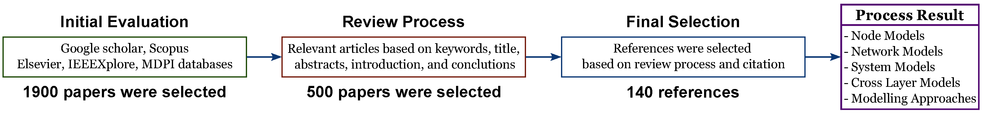
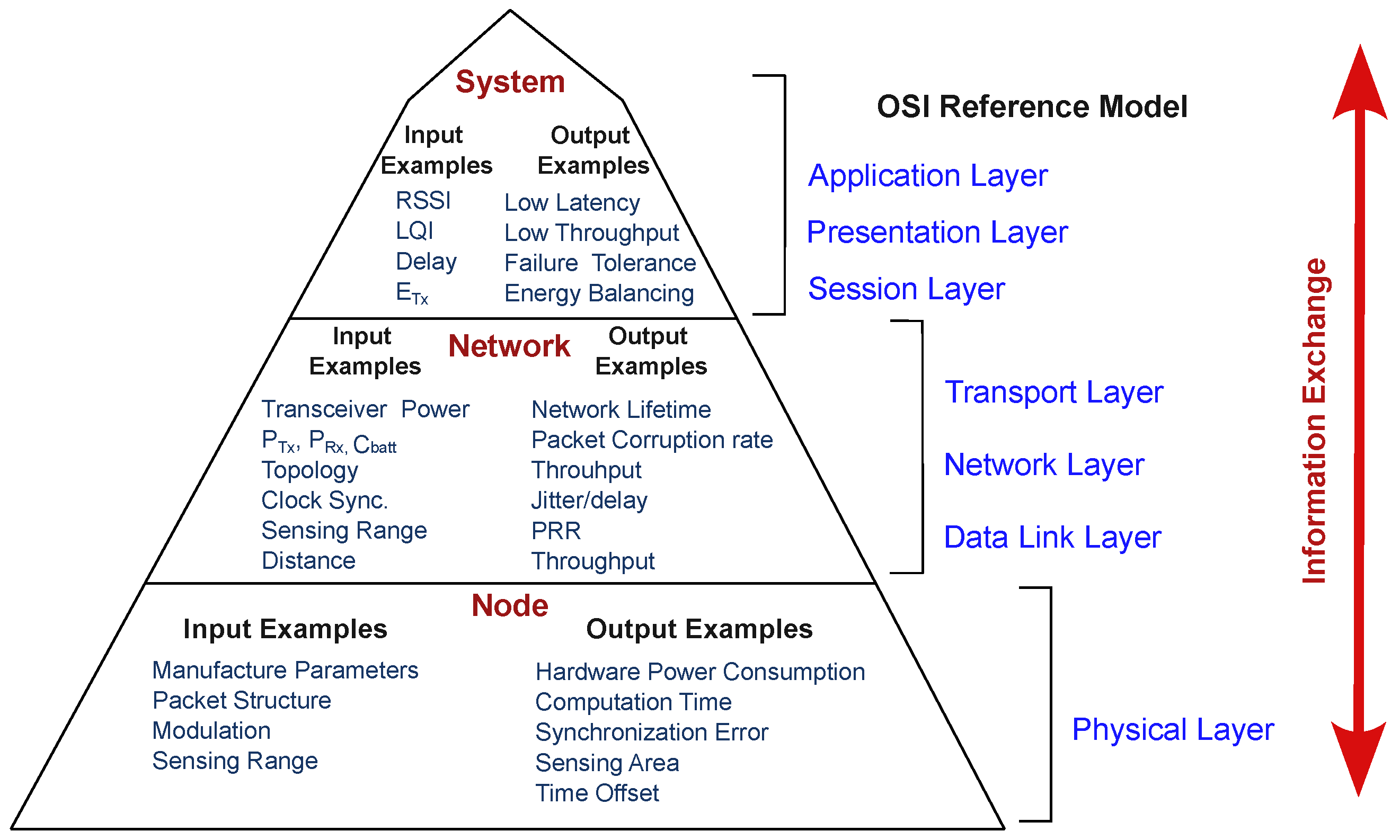
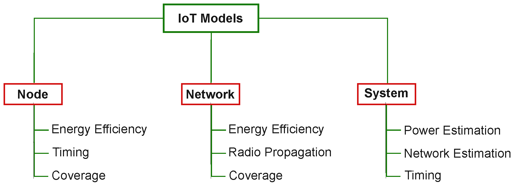
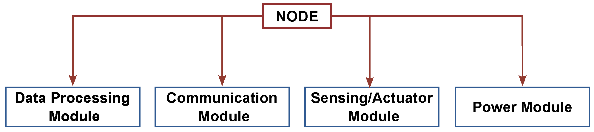
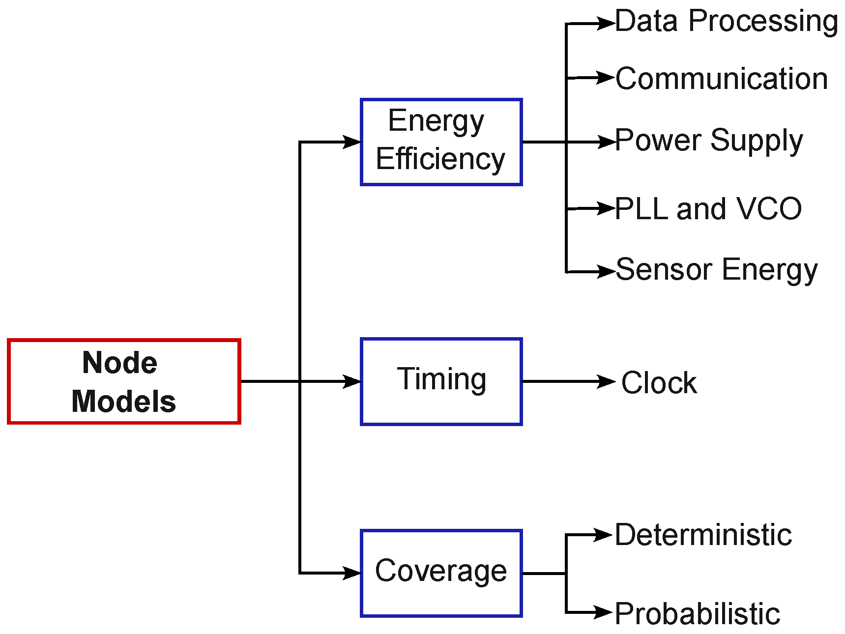
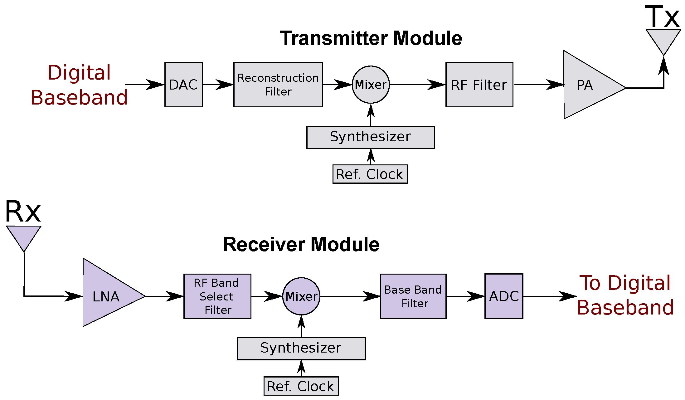
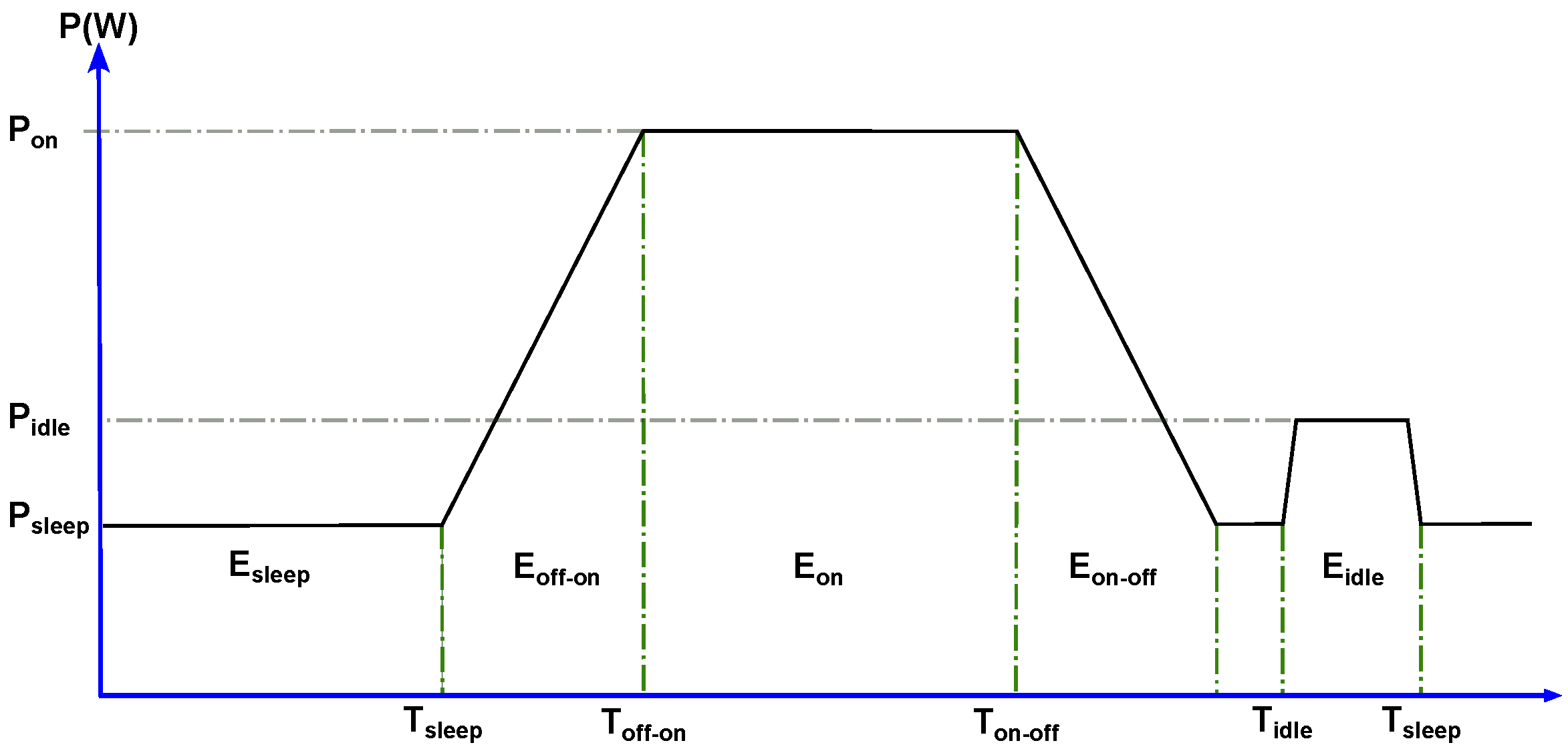
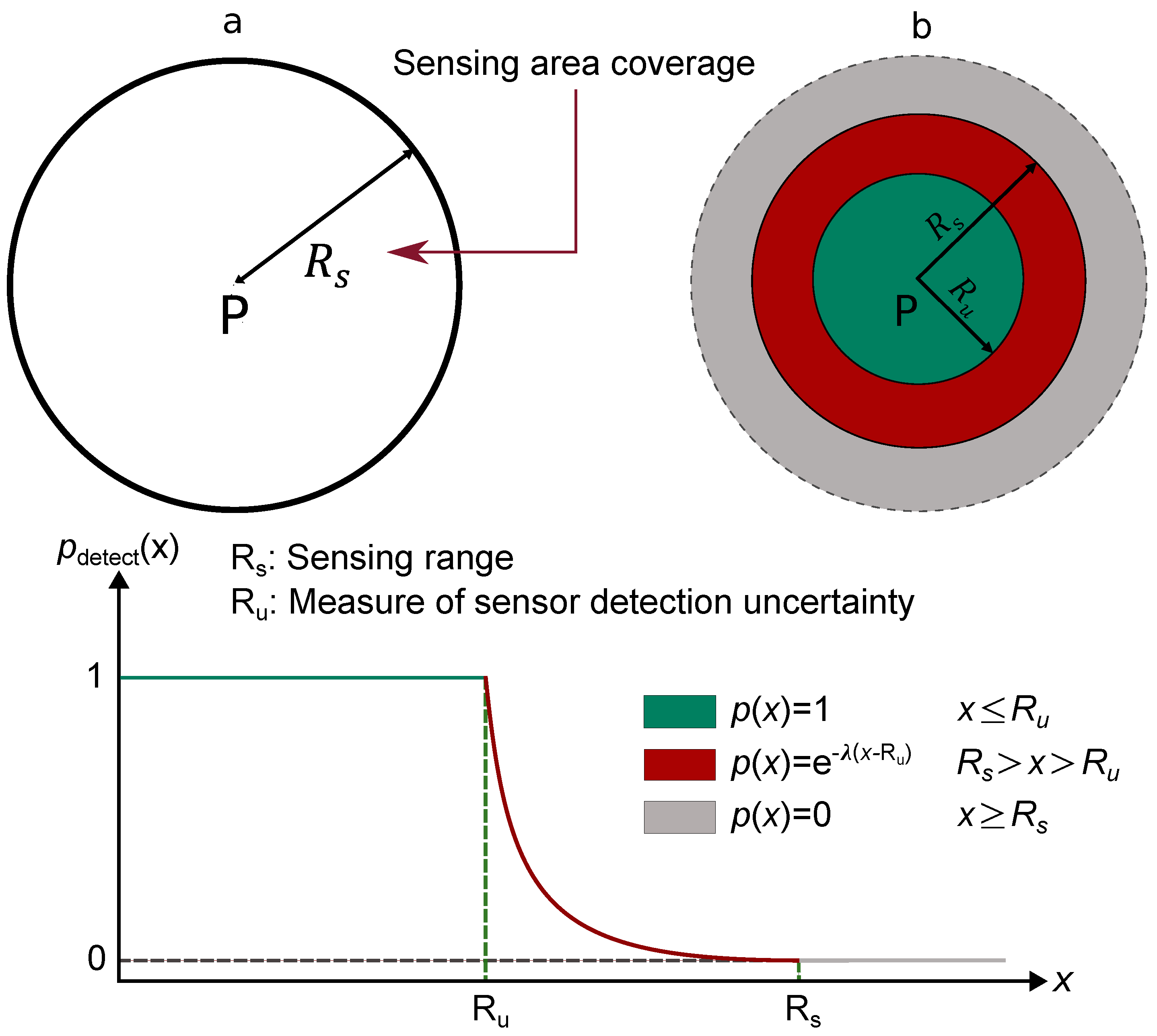
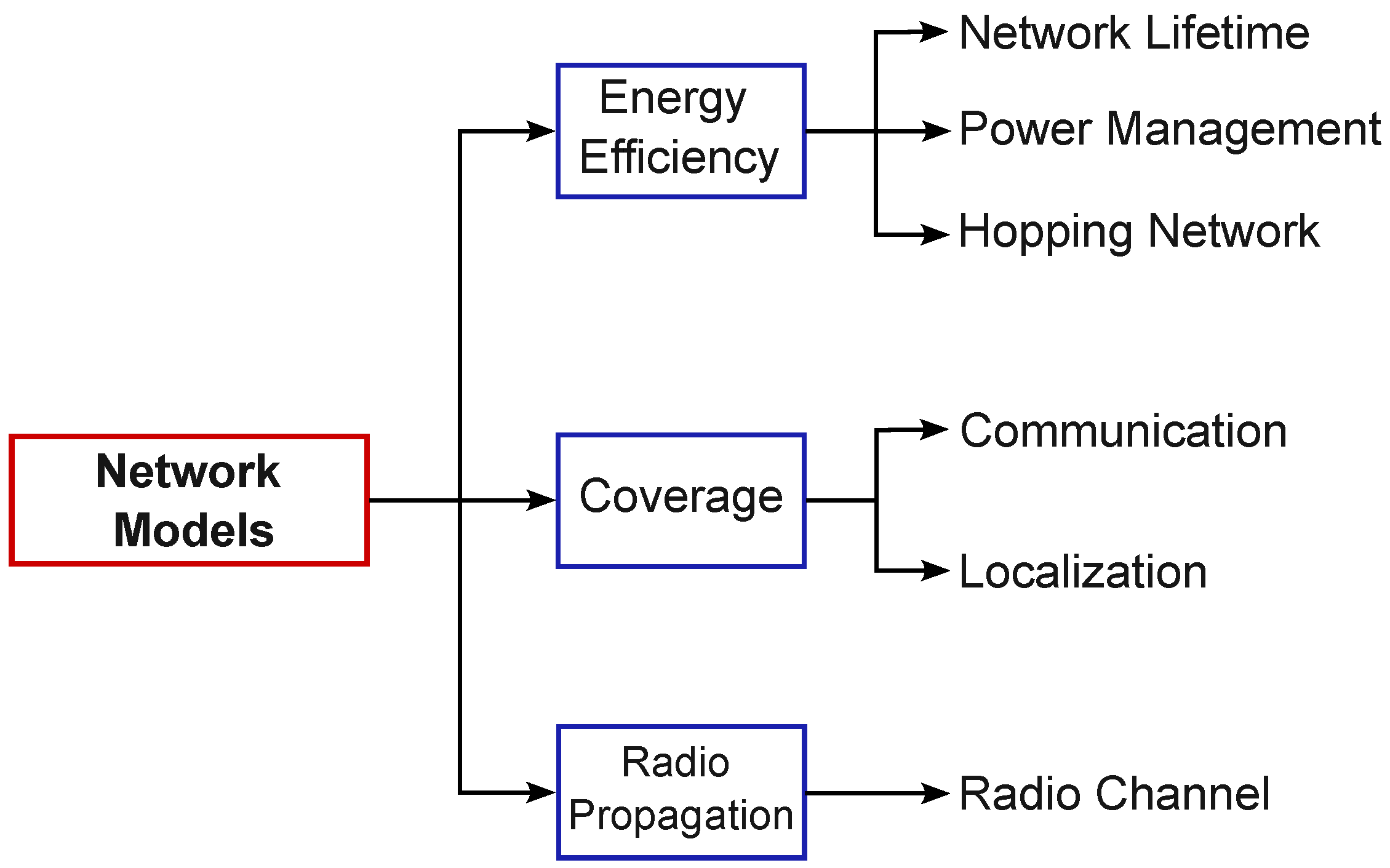
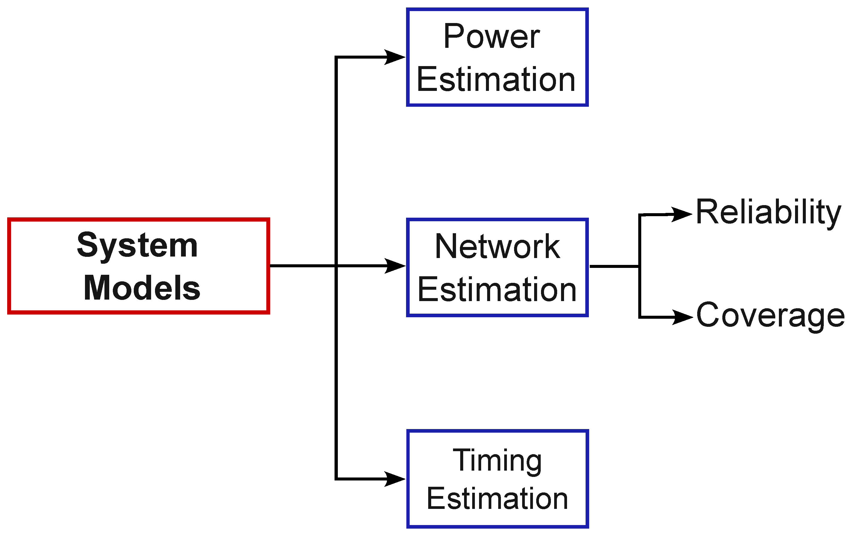
Table 1.
Summary and comparison of node-level models.
| Scheme | Modeling Problem | Modeling Elements | Modeling Methodology | Model | Solution Methodology | Evaluation Approach | Complexity | Models |
|---|---|---|---|---|---|---|---|---|
| Cui et al., 2005 [32] | Power consumption node parameters (maximum transmission time) | Communication medium-related front-end elements | Physical model | Analytical | Optimization (Integer programming problem) | Source code (Solver) | High | Energy Efficiency |
| Li et al., 2006 [5] | Communication node parameters | Communication medium-related front-end elements | Physical model | Analytical | Optimization (Numerical analysis) | Simulation (NS-2) and validation (Implementation) | Medium | Energy Efficiency |
| Zhou et al., 2011 [27] | Power consumption of node components | MCU, RF transceiver, and sensor unit | Physical model | Analytical | System simulation | Simulation (OPENET) | Medium | Energy Efficiency |
| Özkaya et al., 2021 [26] | Power consumption of node components | MCU, RF transceiver, actuator, and sensor unit | Physical model | Analytical | System simulation and validation (Circuit implementation) | Simulation (MATLAB/Simuling and ContikiOS) | High | Energy Efficiency |
| Zhai et al., 2010 [54] | Power consumption node of 4 different front-end architectures | Communication medium-related front-end elements | Physical model | Analytical | Optimization (Numerical analysis) | Simulation (Simulation tools not reported) | Medium | Energy Efficiency |
| Tehrani et al., 2010 [55] | Performance operation of a particular block of the node (PA) | Reference model (mapping PA parameters values) | Generalized memory polynomial (GMP) | Behavioral | Normalized mean square error (NMSE) and Adjacent channel error power ratio (ACEPR) | Simulation (Simulator tools not reported) | High | Energy Efficiency |
| Zahhad et al., 2015 [56] | Power consumption node parameters | Communication medium-related front-end elements | Physical model | Analytical | Optimization (Numerical analysis) | Simulation (NS-2) and validation (Implementation) | Low | Energy Efficiency |
| Zahhad et al., 2016 [35] | Power consumption parameters (Transmitted power) | Communication medium-related front-end elements | Physical models | Analytical | Optimization (Numerical analysis) | Simulation (NS-2) | Low | Energy Efficiency |
| Hou et al., 2017 [57] | - | Phase-locked loop, transmitter and receiver blocks | - | - | Circuit simulation with simulation tool | Implementation on chip (CMOS) | Low | Energy Efficiency |
| Shafique et al., 2017 [58] | Performance operation of a particular block of the node (LNA) | Reference model (mapping LNA parameters values) | Physical model | Behavioral | - | Simulation (MATLAB/Simulink) | Medium | Energy Efficiency |
| Friesel et al., 2018 [59] | Node parameters configuration | Reference model (mapping parameters values) | Training | - | Standard deviation-least square regression | Simulation (Simulation tool not reported) | Low | Energy Efficiency |
| Mahmood et al., 2018 [60] | Power consumption node parameters (Signal to noise ratio (SNR), payload size and modulation order) | Specific block of the transceiver (PA) | Physical model | Analytical | Optimization (Linear programming problem) | Source code (Solver) | High | Energy Efficiency |
| Zhang et al., 2020 [44] | Skew estimation and energy conservation | Transceiver´s clock model | Physical model | Estimation | Source code | Simulation (NS-2) | Medium | Timing |
| He et al., 2017 [45] | Clock synchronization and skew estimation | Transceiver´s clock | Physical model | Estimation | Algorithm | Implementation (Experimental testbed) | Medium | Timing |
| Mahmood et al., 2019 [31] | Power consumption node parameters (Modulation order and transmission time) | Communication medium-related front-end elements | Physical model | Analytical | Optimization (Numerical analysis) | Simulation (Simulation tool not reported) | Medium | Energy Efficiency |
| Jadaa et al., 2020 [61] | Localization | Sensor module | Probability model | Statistical approach | Source code | Simulation (NS-2) | Medium | Coverage |
| Wang et al., 2021 [62] | Efficiency of low power consumption continuous phase frequency shift-keying (CPFSK) transceiver with a frequency-to-amplitude converter (FAC) | Digital controller oscillator (DCO), LNA, FAC, PA | Physical model | - | System simulation | Simulation (Verilog-A) | Low | Energy Efficiency |
| Lacroix et al., 2021 [63] | Efficiency of a particular part of the node (PA) | Communication medium-related front-end elements | Physical model | Analytical | Optimization (Numerical analysis) | Simulation (Simulation tool not reported) | Medium | Energy Efficiency |
| Rasool et al., 2021 [38] | Efficiency of a particular block of the node | Specific block of the node (battery) | Physical model | Analytical | Optimization (Numerical analysis) | Simulation (MATLAB/Simulink) | Low | Energy Efficiency |
| Mini 2021 [46] | Network Coverage | Sensor module | Mathematical model | Binary and probability | Optimization (Numerical analysis) | Simulation (Simulation tool not reported) | Medium | Coverage |
Table 2.
Summary and comparison of network-level models.
| Scheme | Modeling Problem | Modeling Elements | Modeling Methodology | Model | Solution Methodology | Evaluation Approach | Complexity | Model |
|---|---|---|---|---|---|---|---|---|
| Al-Farhani 2021 [81] | Network lifetime | Front-end components | Physical model | - | Algorithm | Simulation (Simulation tool not reported) | Medium | Energy Efficiency |
| Choi et al., 2021 [82] | Network lifetime | Communication medium and node energy consumption parameters | Physical model | Analytical | Optimization (Linear programming problem) | Simulation (MATLAB) | Medium | Energy Efficiency |
| Satyanarayana et al., 2021 [83] | Network Coverage | Sensor module | Mathematical model | - | Algorithm | Simulation (Simulation tool not reported) | Medium | Coverage |
| Mini 2021 [46] | Network coverage | Sensor module | Mathematical model | Probability | Optimization (Numerical analysis) | Simulation (Simulation tool not reported) | Medium | Coverage |
| Zhang et al., 2012 [36] | Energy consumption | RF front-end module | Operation state model | Stochastic | Optimization (Numerical analysis) | Simulation (Simulation tool not reported) | Medium | Energy Efficiency |
| Li et al., 2020 [75] | Network coverage | Sensor module | Physical model | Probability | Probability analysis (Algorithm) | Simulation (Simulation tool not reported) | Low | Coverage |
| Hussein et al., 2020 [84] | Network lifetime | Node energy consumption parameters | Physical model | Analytical | Optimization (Nonlinear multi-variable optimization problem) | Simulation (Mathematica and MATLAB) and validation (implementation) | High | Energy Efficiency |
| Agarwal et al., 2017 [85] | Network lifetime | Sensor node states | Mathematical model | Stochastic | Optimization (Numerical Analysis) | Simulation (MATLAB) | Medium | Energy Efficiency |
| Agrawal et al., 2020 [71] | Network lifetime | Reference model (mapping parameters battery values) | Training | - | Genetic algorithm | Simulation (CAD not reported) and Source code on JAVA | Medium | Energy Efficiency |
| Jadaa et al., 2020 [61] | Localization | Sensor module | Probability model | Statistical approach | Source code | Simulation (NS-2) and implementation of an algorithm | Medium | Coverage |
| Zhou et al., 2019 [86] | Network lifetime | Communication medium and node energy consumption parameters | Operation state model | Analytical | Optimization (Linear programming problem) | Simulation (Simulation tool not reported) | High | Energy Efficiency |
| Kumar et al., 2018 [87] | Network lifetime | Communication medium-related front-end elements | Physical model | Analytical | Source code | Simulation (PEGASIS protocol) | Low | Energy Efficiency |
| Liu et al., 2018 [78] | Localization | Sensor module | Dimensional plane distance | - | Implementation of an algorithm | Simulation | Low | Coverage |
| Kakhandki et al., 2017 [74] | Hop selection | Node energy consumption parameters | Physical model | Analytical | Optimization (Optimal linear problem) | Simulation (SENSORIA) | Medium | Coverage |
| Setiawan et al., 2017 [88] | Network Lifetime | Node energy consumption parameters | Physical model | Analytical | Optimization (Numerical analysis) | Validation (Implementation) | Medium | Energy Efficiency |
| Shakhov et al., 2017 [89] | Network coverage | Sensor module | Physical model | Probability | Optimization (Numerical analysis) | Simulation (Simulation tool not reported) | Medium | Coverage |
| Li et al., 2017 [90] | Network lifetime | Node energy consumption parameters | Estimating model | Probability | Game theory (Nash equilibrium) | Simulation (MATLAB) | Medium | Energy Efficiency |
| Song et al., 2017 [91] | Energy consumption | Reference model (mapping parameters values) | Operation state model | Analytical | Optimization (Numerical analysis) | Simulation (Simulation tool not reported) | Medium | Energy Efficiency |
| Tudose et al., 2013 [73] | Network lifetime | Communication medium-related front-end elements | Physical model | Analytical | Optimization (Numerical analysis) | Simulation (Simulation tool not reported) and implementation of an algorithm | Medium | Energy Efficiency |
| Sharma et al., 2011 [40] | Network lifetime | Node energy consumption parameters | Physical model | Analytical | Optimization (Numerical analysis) | Simulation and validation (Simulation tool and implementation not reported) | Medium | Energy Efficiency |
| Jagriti et al., 2018 [69] | Network Lifetime | RF front-end module and S-MAC protocol | Mathematical model | Analytical | Algorithm | Simulation (MATLAB) | Medium | Energy Efficiency |
| Das et al., 2021 [76] | Coverage and connectivity | Sensor module (sensing and communication radius) | Mathematical model | Probabilistic | Algorithm | Simulation | Medium | Coverage |
Table 3.
Summary and comparison of system-level models.
| Scheme | Modeling Problem | Modeling Elements | Modeling Methodology | Model | Solution Methodology | Evaluation Approach | Complexity |
|---|---|---|---|---|---|---|---|
| Mazloomi et al., 2022 [98] | Power estimation (Network estimation) | Reference model (mapping parameters values) | Vector regression method | - | Optimization (Multiple-objective optimal problem MSOG algorithm) | Simulation (MATLAB) | medium |
| Boardman et al., 2021 [100] | Power estimation (Network lifetime) | Sink, sensor nodes and target nodes | Probabilistic graph | Probability | Optimization (Bi-objective optimal problem) | Simulation (simulation tool not reported), source code (solver) | High |
| Yang et al., 2021 [101] | Power estimation (Network lifetime) | Sink, sensor nodes and target nodes | Stochastic process | Probability | Maximum Likelihood | Simulation (simulation tool not reported) | High |
| Ozkaya 2021 [26] | Power estimation | Sensor nodes components | Physical model | Analytical | Optimization (Numerical analysis) | Simulation (MATLAB/Simulink) | Medium |
| Basabaa et al., 2021 [101] | Power estimation (Harvesting) | Sink, sensor nodes and target nodes | Probabilistic graph | Probability | Algorithm | Simulation (simulation tool not reported) | High |
| Liu 2021 [96] | Coverage estimation (Interference) | Sink, sensor nodes and target nodes | Basic probability assignment | Probability | D-S evidence theory | Algorithm, Simulation (simulation tool not reported) | High |
| Nagar et al., 2020 [99] | Network estimation (Deployment) | Ideal characteristics of IoT devices | Probabilistic | Probabilistic | Optimization (Numerical analysis) | Simulation (MATLAB) | Medium |
| Chakraborty et al., 2019 [97] | Network estimation (Shortest minimal path) | Sink, sensor nodes and target nodes | Probabilistic weight graphs | Probability | Multi-node state reliability evaluator (MNRE) | Simulation (MATLAB) | High |
| Mahmood et al., 2019 [102] | Power estimation | Ideal characteristics of IoT devices (PA) and Gateway | Probabilistic | Probability (QoS) | Optimization (Bi-objective optimal problem) | Source code (Solver) | High |
| Xu et al., 2019 [103] | Coverage estimation (Deployment) | Ideal characteristics of IoT devices and Gateway | Probabilistic node graph model | Analytical and probability | Optimization (Bi-objective optimal problem) | Simulation (MATLAB, Montecarlo method) | High |
| Du et al., 2019 [104] | Power estimation | Ideal characteristics of IoT devices and Gateway | Probabilistic directed acyclic graph | Probability | Optimization (Optimal any path network sub-graph) | Simulation (MATLAB) | High |
| Sarkar et al., 2019 [94] | Network estimation (Cluster-head) | Ideal characteristics of IoT devices and Gateway | Probabilistic | Probability | Optimization (Statistical analysis) | Simulation (MATLAB) | Medium |
| Wang et al., 2018 [105] | Network estimation (Fault estimation) | Sink, sensor nodes and target nodes | Probabilistic functional dependence | Multistate fault tree | Multi-state multi-value decision diagram | Simulation (simulation tool not reported) | High |
| Hasan et al., 2018 [72] | Network estimation (Fault estimation) | Sink, sensor nodes, target nodes | Markov discrete time | Multistate fault tree | Multi-state multi-value decision diagram | Simulation (MATLAB) | High |
| Kassan et al., 2017 [106] | Power estimation (Energy harvesting and battery reliability) | Sensor, node battery, PV-WSN | Binary decision diagram | Probability | Optimization (Numerical analysis) | Simulation (simulation tool not reported) | High |
| Suhonen et al., 2009 [107] | Timing estimation (QoS and duty cycle) | Coverage and deployment | Probabilistic graph | Probability | Optimization (Numerical analysis) | Simulation (NS-2) | Medium |
Table 4.
Comparative perspective of simulation tools frameworks.
| Simulation Tools | Node Models | Network Models | System Models | Core Language | References | ||||||||||||
|---|---|---|---|---|---|---|---|---|---|---|---|---|---|---|---|---|---|
| Circuit | Timing | Node Elements | MAC | Modulation | Topology | IEEE 802.1X Support | Channel | Environment | Routing Protocol | Low latency | Throughput | Time Synchronization | Failure Tolerance | Energy Balance | |||
| Based on Spice | [47] | ||||||||||||||||
| NS-2 | C++ and Otc | [49,108] | |||||||||||||||
| NS-3 | C++ and Python | [109] | |||||||||||||||
| MATLAB/Simulink | High-level programming language | [21] | |||||||||||||||
| OMNET++ | C++ | [110,111,112,113] | |||||||||||||||
| TOSSIM | Python and C++ | [114,115,116,117] | |||||||||||||||
| COOJA (Contiki Os Java) | C++ | [20,118] | |||||||||||||||
| Required Tool | Cross-layer model | ||||||||||||||||
Disclaimer/Publisher’s Note: The statements, opinions and data contained in all publications are solely those of the individual author(s) and contributor(s) and not of MDPI and/or the editor(s). MDPI and/or the editor(s) disclaim responsibility for any injury to people or property resulting from any ideas, methods, instructions or products referred to in the content. |
© 2023 by the authors. Licensee MDPI, Basel, Switzerland. This article is an open access article distributed under the terms and conditions of the Creative Commons Attribution (CC BY) license (https://creativecommons.org/licenses/by/4.0/).
Share and Cite
MDPI and ACS Style
Ojeda, F.; Mendez, D.; Fajardo, A.; Ellinger, F. On Wireless Sensor Network Models: A Cross-Layer Systematic Review. J. Sens. Actuator Netw. 2023, 12, 50. https://doi.org/10.3390/jsan12040050
AMA Style
Ojeda F, Mendez D, Fajardo A, Ellinger F. On Wireless Sensor Network Models: A Cross-Layer Systematic Review. Journal of Sensor and Actuator Networks. 2023; 12(4):50. https://doi.org/10.3390/jsan12040050
Chicago/Turabian StyleOjeda, Fernando, Diego Mendez, Arturo Fajardo, and Frank Ellinger. 2023. "On Wireless Sensor Network Models: A Cross-Layer Systematic Review" Journal of Sensor and Actuator Networks 12, no. 4: 50. https://doi.org/10.3390/jsan12040050
Note that from the first issue of 2016, this journal uses article numbers instead of page numbers. See further details here.