Elliptical and Skew-Elliptical Regression Models and Their Applications to Financial Data Analytics ^†

Abstract

Various statistical distributions have played significant roles in financial data analytics in recent decades. Among these, elliptical modeling has gained popularity, while the study and application of skew-elliptical modeling have garnered increased attention in various domains. This paper begins by acknowledging the notable accomplishments and contributions of Professor Chris Heyde in the field of financial data modeling. We provide a comprehensive review of elliptical and skew-elliptical modeling, summarizing the latest advancements. In particular, we focus on the characteristics, estimation methods, and diagnostics of elliptical and skew-elliptical distributions in regression and time series models, as well as copula modeling. Furthermore, we discuss several related applications in regression and time series models, including estimation and diagnostic methods. The main objective of this paper is to address the critical need for accurately identifying the underlying elliptical distribution, whether it is elliptical or skew-elliptical. This identification is essential for conducting local influence diagnostics and employing appropriate regression methods using suitable elliptical modeling techniques. To illustrate this process, we present examples that demonstrate the identification of the elliptical distribution, starting with the Box–Jenkins methodology and progressing to copula modeling. The inclusion of copula modeling is motivated by its effectiveness in conjunction with elliptical and skew-elliptical distributions, as it aids in distinguishing between the two. Ultimately, the findings of this paper offer valuable insights, as correctly determining the elliptical and skew-elliptical distribution enables the application of suitable local influence and regression methods, thereby contributing to financial portfolio management, business analytics, and insurance analytics, ensuring the accurate specification of models.

1. Introduction

This paper draws inspiration from the pioneering work of Professor Chris Heyde in the field of financial data modeling. Our objective is to provide a comprehensive review of elliptical and skew-elliptical regression methods, highlighting recent developments in this area. Additionally, we introduce copula modeling as a methodology that facilitates the identification between an elliptical and skew-elliptical distribution, thereby aiding in model selection.

Professor Chris Heyde (1939–2008) was a distinguished mathematician, statistician, and scientist from Australia. Throughout his eminent career, he received numerous honors, including being elected Fellow of the Australian Academy of Science (1977) and the Academy of the Social Sciences in Australia (2003), as well as being presented the Member of the Order of Australia (AM) in 2003. Highly regarded by his colleagues and students, Professor Heyde made significant contributions to various areas of Probability, Statistics, and Stochastic Analysis, with applications in finance and other real-world areas. To celebrate his 65th birthday and his remarkable achievements, a special volume edited by Gani and Seneta (2004) was dedicated to him. The volume featured contributions from over 50 collaborative authors and included 30 papers. It was presented to Professor Heyde during a conference held in his honor at the Australian National University, Canberra. His perspectives on different areas and future directions were captured in an interview by Glasserman and Kou (2006). Furthermore, Maller et al. (2010) compiled and commented on Professor Heyde’s selected works, while Seneta and Gani (2009) provided an introduction to his life and work.

Among Professor Heyde’s achievements, he focused on studying the distributional characteristics and tail behaviors of financial data, as evidenced by notable publications, such as Heyde (1967; 1999), and Maller et al. (2010). One of his seminal papers is undoubtedly Heyde (1999). Another significant contribution, destined to become a classic, was his later publication with N. N. Leonenko in Heyde and Leonenko (2005). These works were built upon his firm and longstanding belief that the generalized t-distribution, with its power-law tails, represented the appropriate distribution for his model in studying stock market returns. Supported by Columbia University, Professor Heyde obtained a US Patent, derived from this research. It is his profound interest in financial data that strongly motivated us to present this paper, see Heyde (1999).

Within various disciplines such as business, economics, finance, insurance, and related fields, one can find symmetric, elliptical, skew-elliptical, and various other distributions, as well as their corresponding regression and time series models. Examples of such works include Heyde and Liu (2001); Liu and Heyde (2008); Liu et al. (2011, 2015, 2020, 2022a), and Fung and Seneta (2021). Elliptical and skew-elliptical regression models find applications in statistical inference, sensitivity analysis, local influence diagnostics, and other areas. However, estimating these models poses challenges due to the difficulties in obtaining maximum likelihood estimates for skew-elliptical distributions.

Given the growing interest in multivariate elliptical and skew-elliptical distributions, many authors have derived characteristic functions for these distributions, as noted in Dong and Yin (2021). This highlights the necessity of determining the underlying elliptical or skew-elliptical distribution when conducting regression modeling. Since elliptical and skew-elliptical distributions are composed of normal (symmetrical) or skewed (asymmetrical) distributions, or combinations thereof, it can be challenging to identify a suitable regression methodology for a given elliptical distribution. In this paper, we delve into the identification of elliptical and skew-elliptical distributions and explore their applications in finance and insurance. Furthermore, we examine their utilization in the literature and expand on model selection methods.

We emphasize the significance of selecting the appropriate regression modeling methodology, whether it be elliptical or skew-elliptical, and explore the associated issues and implications when employing these methods for the respective distributions. This exploration has led us to investigate time series and copula modeling techniques. We initiated our study with the Box–Jenkins methodology, where we developed a univariate GARCH-type model as a means to identify elliptical distributions. Subsequently, we delve into bivariate copula modeling, which serves as a methodology for identifying the underlying distribution to be modeled, whether it is elliptical or skew-elliptical.

Throughout this paper, we identify several statistical distributions, regression models, and time series models that find applications in the analysis of financial and insurance data, utilizing elliptical and copula regression methods. We emphasize the importance of copula modeling as a methodology for identifying the distribution, thereby aiding in model selection. The structure of this paper is as follows: In Section 2, we provide a brief review of various statistical distributions and their associated models used in financial data analytics. In Section 3, we delve into elliptical and skew-elliptical models. Section 4 focuses on different regression methods, while Section 5 discusses elliptical regression diagnostics. In Section 6, we explore copula regression. In Section 7, we present several illustrative examples, and finally, in Section 8, we conclude with our remarks.

2. The Big Picture

The use of various statistical distributions, along with their associated regression and time series models, is established across multiple domains such as business, economics, finance, insurance, and related disciplines. A wealth of research results in this area can be found in publications including Kariya and Sinha (1989); Fang and Anderson (1990); Fang and Zhang (1990); Genton (2004); Gupta et al. (2013); Liu and Sathye (2021), and SenGupta and Arnold (2022).

In portfolio management, the estimation of correlation plays a central role in assessing the risk–return trade-off associated with investment portfolios. Low correlation is desirable from a diversification perspective, as it enhances the benefits of portfolio diversification, see Campbell et al. (2002). Accurate correlation estimates are crucial for effective portfolio management, as increased correlation during turbulent market conditions diminishes the advantages of diversification, see Campbell et al. (2008).

The literature extensively explores multivariate elliptical regression models. Notable studies in this area include Lange et al. (1989); Welsh and Richardson (1997), and Fernández and Steel (1999). Among the various types of elliptical regression models, symmetric elliptical regression is the most commonly studied, as its parameters can be easily estimated. Examples of such models include the Student’s t-distribution, power exponential distribution, and contaminated normal distribution, each exhibiting tails that are heavier or lighter than those of the normal distribution, see e.g., Lemonte and Patriota (2011); Liu (2004), and Liu et al. (2011).

In the not-too-distant past, a common assumption in financial time series modeling was that errors were mutually independent and followed a normal distribution. However, financial data often exhibit skewed distributions and heavy-tailed errors; see Genton (2004); Liu and Sathye (2021); Liu et al. (2020, 2022a, 2022b, 2023), and Ma et al. (2005). As a result, heavy-tailed distributions have gained popularity in financial modeling to capture these characteristics. The Student’s t-distribution, with varying degrees of freedom, has been a focus in financial modeling due to its ability to accommodate a wide range of power-tail possibilities, including the Cauchy distribution $(v=1)$, and approaching the Gaussian distribution as $v\to \infty$, see Heyde and Leonenko (2005).

In recent years, there has been increasing interest and research attention on skew distributions. Various skew distributions, such as skew–normal, skew-Student’s t, and skew Laplace, have been proposed and studied. It is now well-documented that financial data can exhibit errors with skewed distributions, see Liu and Sathye (2021); Wichitaksorn et al. (2014) and Liu et al. (2022b).

Real-world financial data often display asymmetry and fat tails, making it unsuitable to be approximated by normal or symmetric distributions. Additionally, financial data exhibit volatility clustering, as evidenced by the presence of asymmetries in volatility, correlations, and stock return beta. Recent studies have highlighted these asymmetric characteristics, including asymmetries in stock return beta, asymmetric correlations and their applications in financial markets, see Arellano-Valle and Azzalini (2013); Bekaert and Wu (2000); Black (1976), and Cao et al. (2023).

The investigation of asymmetries in asset allocation decisions in an out-of-sample setting has been a topic of interest. Patton (2004) explored the economic and statistical significance of asymmetries and their impact on asset correlation during economic downturns. It was found that traditional allocation criteria based on asset correlation may be inadequate in the presence of cyclicality and asymmetry. Patton’s study showed that a model capturing skewness and asymmetric dependence led to better portfolio decisions compared to a bivariate normal model.

To analyze datasets that exhibit non-normal features, including asymmetry, multimodality, and heavy tails, there has been a growing need for more flexible tools. This has led to the development of non-normal model-based methods, see Lee and Mclachlan (2013). Skew distributions and their finite mixtures have emerged as alternatives to symmetric and Gaussian mixture models, following the influential work by Azzalini and Capitanio (2013) and Azzalini and Dalla Valle (1996). Determining the appropriate modeling methodology, whether it is elliptical or skew-elliptical, is crucial for ensuring correct model specification in such cases.

2.1. GARCH Formulations

Mostly associated with financial modeling are GARCH-type (forecasting) models, see Cao et al. (2023); Liu (2004); Liu and Heyde (2008); Liu et al. (2011, 2022b), and Dewick (2022). These models provide a framework for modeling financial volatility and can capture symmetric or asymmetric effects. They are widely used to identify and capture the stylized facts present in financial data, characterized by volatility clustering and high kurtosis, which have a significant impact on financial modeling; see Ghani and Rahim (2019).

GARCH-type models are employed for analyzing and forecasting volatility, offering flexibility in capturing volatility clustering and asymmetries within the data, see Dewick (2022). The family of GARCH models includes various formulations, such as exponential GARCH (EGARCH), Glosten Jagannathan–Runkle GARCH (GJR–GARCH), threshold GARCH (TGARCH) models, etc. These models allow for the modeling of both symmetric and skewed distributions, providing a versatile toolkit for financial modeling and analysis, see Dewick (2022).

For detailed formulations of common GARCH-type models, please refer to Dewick (2022).

2.2. Copula Formulations

In this subsection, we begin by examining the development of Copula modeling and then delve into its application in elliptical and skew-elliptical regression. Copula modeling, also known as dependence modeling, revolves around a fundamental concept, see Stamatatou et al. (2018). It involves decomposing a joint distribution function into two independent parts: one describing the marginal or univariate behavior and the other capturing the dependence structure. The role of the copula function is to combine the two univariate marginal distributions in a manner that preserves their individual characteristics and provides a measure of dependence without the need to specify a prior joint distribution. Instead, the probability integral transformation is employed to convert the marginal distributions into uniform distributions, and the joint relationship is subsequently modeled using a copula function, see Vuolo (2017).

Table 1. Important Copula Publications.

Author (Year)	Paper/Book/Thesis
Sklar (1959)	Fonctions Derépartitionàn Dimensions et Leurs Marges.
Embrechts et al. (2001)	Modelling Dependence with Copulas.
Cherubini et al. (2004)	Copula Methods in Finance
Patton (2006)	Modeling Asymmetric Exchange Rate Dependence.
Nelsen (2007)	An Introduction to Copulas.
Christoffersen et al. (2012)	Is the Potential for International Diversification Disappearing? A Dynamic Copula Approach.
Joe (2014)	Dependence Modeling with Copulas.
Hofert et al. (2018)	Elements of Copula Modeling with R.

presents a compilation of significant publications related to copula modeling.

Copula modeling has proven to be a valuable tool for analyzing highly dependent phenomena, as demonstrated in various areas, such as financial market performance, market confidence, and market speculation, see Gródek-Szostak et al. (2019). Numerous studies have highlighted the effectiveness of copula models in characterizing the joint dependence among variables, particularly when extreme values are prominent, see Bhatti and Do (2019).

The concept of copula modeling has been discussed in several texts, with notable contributions from Hoeffding, see e.g. Nelsen (2007). Hoeffding studied measures of dependence that remain invariant under strictly increasing transformations. However, it was Sklar (1959) who made the most significant contribution by introducing the notation and terminology of a copula, as stated in Theorem 1.

Theorem 1 

(Sklar’s Theorem (Sklar 1959)). Let F be an n-dimensional joint cumulative distribution function for the random variables $X_1,X_2,\dots ,X_n$ with marginal distribution functions $F_1\left(x_1\right),F_2\left(x_2\right),\dots ,F_n\left(x_n\right)$, then there exists a copula function C, such that

$$F_{x_1,...,x_n}(x_1,\dots ,x_n)=C[F_1\left(x_1\right),\dots ,F_n\left(x_n\right)]$$

(1)

when the marginal distributions are continuous, then C is unique. If any distribution is discrete, the C is uniquely defined by the support of the joint distribution, see Parsa and Klugman (2011).

Copulas are divided into copula families and are classified according to their distributional properties. Elliptical and Archimedean copulas can be classified as implicit copulas, such as Gaussian and Student’s t copulas. Explicit copula examples are Clayton, Frank, and Gumbel types; see Kayalar et al. (2017). An Archimedean copula is a copula of the form:

$$C\left(u\right)=\psi ({\psi }^{-1}\left(u_1\right)+\dots +{\psi }^{-1}\left(u_d\right)),u\in {[0,1]}^d$$

(2)

where the so-called generator function $\psi$ is defined by, e.g., Hofert et al. (2018).

Although the elliptical and Archimedean copulas are implicit, elliptical copulas can use Pearson’s linear correlation, Kendall’s $\tau$, or Spearman’s $\rho$ for the measures of association. Archimedean copulas use Kendall’s $\tau$ or Spearman’s $\rho$ as their measure of association, see Vuolo (2017). For the linear copula regression functions, the coefficients will be related to Pearson’s correlation, see Sungur (2006), which is required for the estimation of their maximum likelihood estimates.

2.3. GBM and FATGBM Models

Apart from the GARCH and Copula formulation, many other methods are available when exploring the asymmetric positive returns of financial data. These models can include the geometric Brownian motion (GBM) model, see Dewick (2022). The GBM model is commonly used for modeling the price of a risky asset. The success of Black and Scholes in obtaining an analytical pricing formula using the GBM model has significantly influenced the option pricing industry, see Heyde and Liu (2001). In the mathematical finance paradigm, the price $P_t$ at time t of a risky asset can be represented as

$$P_t=P_{0}exp[\mu t+\sigma W\left(t\right)]$$

(3)

where $P_0$ is the stock price or index value at time 0, drift $\mu$ and scale $\sigma >0$ are fixed constants, and $W\left(t\right)$ is a standard Brownian motion, see Dewick (2022). The corresponding log returns can be expressed as follows:

$$X_t=log{P}_t-log{P}_{t-1}=\mu +\sigma (W\left(t\right)-W(t-1))$$

(4)

which are i.i.d. Gaussian.

Professor Heyde (1999) proposed a GBM with the fractal activity time (FATGBM) model; see also Gupta et al. (2021); Heyde et al. (2001); Heyde and Liu (2001); Kerss et al. (2014); Leonenko et al. (2012); Madan and Schoutens (2020), and Meerschaert and Sikorskii (2019) for detailed studies. The FATGBM model aims to generalize the GBM model, Equation (3), see Heyde et al. (2001).

$$P_t=P_{0}exp[\mu t+\sigma W\left(T_t\right)]$$

(5)

where $P_t$ is the stock price or index value at time t, $\mu$ is the long-term drift, $\sigma$ is a parameter that determines volatility scaling and $T_t$ is the “fractal activity time” independent of the Brownian motion $W\left(\right)$.

3. Elliptical and Skew-Elliptical Distributions

In about 1886, when Francis Galton first examined the relationship between heritable traits of parents and their offspring, he observed that the contours of equal bivariate frequencies in the joint distribution formed concentric shapes resembling ellipses, varying only in size; see also Friendly et al. (2013). Since then, elliptical distributions have found their application in financial modeling.

An elliptical distribution, whether symmetrical or skew-symmetrical, refers to a d-dimensional random vector, as defined in Definition 1. In financial time series analysis, it may be necessary to stabilize the data, which can be achieved by taking the log-difference of the time series and considering the resulting residuals as approximately following a standard normal distribution or by using the Box–Jenkins methodology, see Dewick (2022). Distributions commonly found in finance possess distinctive features or characteristics that require appropriate modeling methods.

Several methods are commonly employed to model these features. The most prevalent ones include the use of elliptical distributions, which have garnered significant attention in the literature, see Fang and Anderson (1990); Fang and Zhang (1990); Galea et al. (1997); Kariya and Sinha (1989); Liu and Heyde (2008), and Liu et al. (2011). This family of symmetric distributions encompasses various members, such as the normal, Student’s t, contaminated normal, and logistic distributions, among others, see Azzalini and Dalla Valle (1996); Azzalini and Capitanio (2013), and Landsman et al. (2003). The elliptical class offers a useful extension of the normal model as it encompasses both light-tailed and heavy-tailed distributions for the errors, see Osorio et al. (2007). Definition 1 provides the fundamental concept of the elliptical distribution.

Definition 1

(Elliptical Distributions). A d-dimensional random vector X has an elliptical distribution with the location vector $\mu \in {\mathbb{R}}^d$, scale (or dispersion) matrix $\Sigma =A{A}^{\prime }$ with rank $(\Sigma )=k\le d$ for a matrix $A\in {\mathbb{R}}^{d\times k}$, and a radical part $R\ge 0$, if

$$X\stackrel{d}{=}\mu +AYforY\stackrel{d}{=}RS$$

(6)

where $\stackrel{d}{=}$ is equal in distribution, $S\sim U\left(\right\{x\in {\mathbb{R}}^k:\parallel x\parallel =1\left\}\right),\parallel ·\parallel$ denotes the Euclidean norm (that is, S is uniformly distributed on the unit sphere in ${\mathbb{R}}^k$) and R and S are independent. The distribution of Y is known as the spherical distribution, see Hofert et al. (2018).

Further to the definition of an elliptical distribution shown in Definition 1, the elliptical distribution can be defined as either symmetrical, refer to Definition 2, or as a skew-elliptical, refer to Definition 3.

Definition 2

(Symmetrical Elliptical Distributions). An $n\times 1$ random vector, Y, has an elliptical distribution with an $(n\times 1)$ location parameter, μ, and an $(n\times n)$ scale matrix, Σ, if its density function is

$$f_Y\left(y\right)={|\Sigma |}^{-1/2}g\left[{(y-\mu )}^{\top }{\Sigma }^{-1}(y-\mu )\right],y\in {\mathbb{R}}^n$$

(7)

where the function $g:\mathbb{R}\to [0,\infty ]$ is such that ${\int }_0^{\infty }{u}^{n-1}g\left(u^2\right)du<\infty$. The function $g(·)$ is typically known as the density generator, see Galea et al. (2000).

For a vector Y distributed according to the density at Equation (7), we use the notation $Y\sim E{l}_n(\mu ,\Sigma ,g)$, or simply, $Y\sim E{l}_n(\mu ,\sigma )$. In the case where $\mu =0$ and $\Sigma =I$, we obtain the spherical family of densities. Note that $c_1,c_2,\cdots ,c_6$ in

Table 2. Elliptical Distributions’ Generating Function [for the source of original information, please refer to Galea et al. (2000); permission granted by the Brazilian Journal of Probability and Statistics].

Distribution	Notation	Generating Function—$\mathit{g}(·)$
Normal	$N_n(\mu ,\Sigma )$	$g\left(u\right)=c_1{e}^{-u/2}$, $u\ge 0$
Student’s t	$t_n(\mu ,\Sigma ,v)$	$g\left(u\right)=c_2{(1+u/v)}^{-(v+n)/2},u\ge 0$
Contaminated Normal	$C{N}_n(\mu ,\Sigma ,\delta ,\tau )$	$g\left(u\right)=c_3\{(1-\delta )e^{-u/2}+\delta {\tau }^{-n/2}{e}^{-u/\left(2\tau \right)}\},u\ge 0$
Cauchy	$C_n(\mu ,\Sigma )$	$g\left(u\right)=c_4{(1+u)}^{-(n+1)/2},u\ge 0$
Logistic	$L_n(\mu ,\Sigma )$	$g\left(u\right)=c_5{e}^{-u}/{(1+e^{-u})}^2,u\ge 0$
Exponential Power	$P{E}_n(\mu ,\Sigma ,\alpha )$	$g\left(u\right)=c_6{e}^{-u^{\alpha }/2},u\ge 0$

are used to denote normalizing constants, see Galea and Giménez (2019); Galea et al. (1997, 2000, 2003). Symmetrical elliptical distributions have a generating function $g(·)$, see Table 2. This generating function allows for the estimation of the distribution’s parameters.

Common skew-elliptical distributions are the skew–normal and skew-Student’s t; see a recent overview by Azzalini (2022). The symmetrical elliptical distributions are estimated using a generating function, $g(·)$, listed in Table 2. This feature is not available when modeling for skew-elliptical distributions. Instead of using the generating function, $g(·)$, skew-elliptical distributions typically use an expectation–maximization (EM) methodology in estimating the distribution parameters. The definition of the skew-elliptical distribution is given in Definition 3.

Definition 3

(Skew-Elliptical Distributions). The skew-elliptical formulation involves a d-dimensional symmetric density $f_0\left(x\right)$, such that $f_0(-x)=f_0\left(x\right)$, with $w(-x)=-w\left(x\right)$. G represents the distribution function of a scalar random variable that is symmetrically distributed around 0 for all $x\in {\mathbb{R}}^d$, see Arellano-Valle and Azzalini (2013), to generate a whole set of perturbed versions of $f_0$ via the expression

$$f\left(x\right)=2f_0\left(x\right)G\left\{w\left(x\right)\right\},x\in {\mathbb{R}}^d$$

(8)

The skew-elliptical distribution, see Arellano-Valle and Azzalini (2013) and Azzalini (2022), constitutes a broad set of probability distributions with a d-dimensional symmetric density $f_0\left(x\right)$, such that $f_0=f_0\left(x\right)$ for all $x\in {\mathbb{R}}^d$, to generate a set of perturbed versions of $f_0$ via the expression.

The skew–normal family is a more flexible class of distributions because of the additional parameter $\alpha$, which regulates skewness, see Arellano-Valle and Azzalini (2013) and Equation (9). The additional parameter $\alpha$ is to regulate the skewness in the univariate case with a density function $x(x\in {\mathbb{R}}^d)$ is

$$\frac{2}{\omega }\phi \left(z\right)\varphi \left(\alpha z\right),z=\frac{x-\xi }{\omega }$$

(9)

where $\phi$ and $\varphi$ denote the $N(0,1)$ density function, and $\xi ,\omega$, and $\alpha$ are parameters, which regulate location, scale, and shape $(\omega >0)$, see Arellano-Valle and Azzalini (2013).

Although more flexible than the normal family, the skew–normal family cannot adequately handle distributions with thicker tails than the normal ones. In order to deal with thicker tails, the skew–normal distribution with its scalar mixtures is an appealing alternative, see Liu and Sathye (2021). Some important publications are listed in the following

Table 3. Selected publications of skew-elliptical distributions.

Author (Year)	Paper/Book/Thesis
Azzalini and Dalla Valle (1996)	The Multivariate Skew–Normal Distribution.
Arellano-Vale and Genton (2010)	Multivariate Unified Skew-Elliptical Distributions.
Adcock and Azzalini (2020)	A Selective Overview of Skew-Elliptical and Related Distributions and of their Applications.
Azzalini (2022)	An Overview on the Progeny of the Skew-Normal Family—A Personal Perspective.
Kwong and Nadarajah (2022)	A New Class of Skew Elliptical Distributions.
Liu et al. (2023)	Robust Autoregressive Modeling and its Diagnostic Analytics with a COVID-19
	Related Application.

.

4. Elliptical and Skew-Elliptical Regression

Since the linear regression coefficient functions are related to Pearson’s correlation, see Sungur (2006), developments in models and strategies have allowed for the modeling of heavy-tailed data using non-normal, skew-elliptical distributions, see Li et al. (2022). Moreover, a generalized class of univariate skew distributions can be constructed by partitioning a two-scaled mixture of normal distributions, see Wichitaksorn et al. (2014) for examples. Strategies for skew-elliptical regression include using median and quartile regression for both skew-elliptical and copula regression, which are presented as follows.

4.1. Elliptical Regression

Firstly, a typical linear regression model can be given as

$$Y=X\beta +ϵ$$

(10)

where Y is an $n\times 1$ vector of responses, X is a known $n\times p$ matrix of rank p, $\beta$ is a p-dimensional vector of responses, and $ϵ$ is a p-dimensional error vector following an elliptical distribution $Y\sim E{l}_n(0,\varphi I)$, where $\varphi$ is the scale parameter, see Galea et al. (2000).

Definition 4

(Elliptical Regression). An elliptical regression model in its generalized form can be defined as

$$Y\sim E{l}_n(X\beta ,\eta I)$$

(11)

If the generating function is a continuous and decreasing function, see Table 2, then the maximum likelihood estimators of β and η are

$$\widehat{\beta }={\left(X^{\top }X\right)}^{-1}{X}^{\top }Y\mathrm{and}\widehat{\eta }=Q\left(\widehat{\beta }\right)/u_0$$

(12)

where $Q\left(\beta \right)={(Y-X\beta )}^{\top }(Y-X\beta )$ and $u_0$ maximize the function, see Galea et al. (2000).

Note that for the normal and Student’s t-distributions, $u_0=n$. For the exponential distribution, $u_0={(n/\alpha )}^{1/\alpha }$. For the contaminated normal and logistic distributions, $u_0$ needs to be obtained numerically. For the logistic distribution, $u_0$ is given as

$$\frac{n}{2u}=\tanh \left(\frac{u}{2}\right)$$

(13)

An important issue for the regression model is the choice of the distribution. It may be that the choice of the distribution of $ϵ$ is usually restricted to standard distributions, such as normal or Student’s t-distributions, see Branco and Dey (2002). Elliptical regression is convenient due to the closed form of the elliptical distribution.

4.2. Skew-Elliptical Regression

The association between two continuous variables mostly includes Pearson’s $\rho$, Spearman’s $\rho$, and Kendall’s $\tau$. A common practice is to discretize variables at one or several representative quantiles, and then evaluate the association based on the resulting contingency table. By summarizing the dependence at one or several representative quantiles, such as the median or quartiles, one may obtain an alternative quantification of the overall association. Association measures that are indexed by quantiles can provide a clearer view of the local association structure when the bivariate outcomes have different locations or scales, see also Liu and Sathye (2021); Liu et al. (2020, 2022a), and references therein.

Median and Quantile Association Regression

Quantile regression is used for the estimation of conditional quantiles of a response, given a vector of regressors. Quantile regression can be used to measure the effect of regressors, not only in the center of a distribution, but also in the upper and lower tails, see Guan et al. (2008). Quantile regression has more advantages over classical regression in analyzing financial data with heavy tails as it provides more information, see Guan et al. (2008). For the description of quantile copula modeling of an Archimedean class of copula, see Guan et al. (2008).

5. Elliptical and Skew-Elliptical Regression Diagnostics

Within financial modeling, the capital asset pricing model (CAPM) is considered one of the most important asset pricing models in financial economics. The CAPM is widely used in estimating the cost of capital for companies and in the measurement of portfolio performance, see Galea and Giménez (2019). Further, the vector autoregressive (VA) and GARCH models are important in studying multiple time series models used throughout economics and finance, see Liu et al. (2015). To this end, sensitivity analysis (diagnostics) is used to evaluate the stability of a model to perturbations (deviations) within the data.

The deletion of outliers and influential returns is an important stage of any financial model to enable an evaluation of the sensitivity of the results since atypical returns can distort the estimators and results, see Galea and Giménez (2019). Influential observations within a model may exist or overlap in the mixture rather than in isolation. It would be inappropriate to apply case deletion as the dependency structure of the autoregressive model, e.g., the GARCH model, see Liu (2004). An alternate methodology is to examine the local change in the autoregressive parameter estimate caused by a small perturbation associated with observations. Cook (1986) proposed a methodology called local influence. The method of local influence is a general diagnostic tool for assessing the effect of local departures from model assumptions and has been extensively applied to various areas, see Galea et al. (1997).

Since Cook (1986) introduced the local influence approach, it has extensively been applied to various areas. This approach consists of three main concepts, mainly a likelihood displacement $\left(LD\right)$ along with its influence graph $\alpha$ and a normal curvature $C_l$, see Liu (2004). Local influence can use several methods in estimation, such as elliptical regression and tests of mean-variance efficiency, see Galea and Giménez (2019). The definition of local influence is given in Definition 5.

Definition 5

(Local Influence on the Likelihood Displacement). Let $L\left(\theta \right)$ denote the log-likelihood function from the postulated model and let ω be a $q\times 1$ vector of permutations restricted to some subset $\Omega \subset {\mathbb{R}}^q$. The perturbations are made on the likelihood function to take the form $L\left(\theta \right|\omega )$. Denoting the vector of no perturbation by ${\omega }_0$, we assume $L\left(\theta \right|{\omega }_0)=L\left(\theta \right)$. To assess the influence of the perturbations on the maximum likelihood estimate $\widehat{\theta }$, one may consider the likelihood displacement

$$LD\left(\omega \right)=2\{L\left(\widehat{\theta }\right)-L\left({\widehat{\theta }}_{\omega }\right)\}$$

(14)

where ${\widehat{\theta }}_{\omega }$ denotes the maximum likelihood estimate under the model $L\left(\theta \right|\omega )$, see Galea et al. (2003).

The likelihood function under the postulated model is given as

$$L\left(\theta \right)=log\left[\right|\varphi I_n{|}^{-1/2}g\left\{{(y-X\beta )}^{\top }{\left(\varphi I_n\right)}^{-1}(y-X\beta )\right\}]=-\frac{n}{2}log\varphi +logg\left(u\right)$$

(15)

where $u=Q\left(\beta \right)/\varphi$ and $\theta ={({\beta }^{\top },\varphi )}^{\top }$, with ${\left(\right)}^{\top }$ denoting the transpose of the vector, see Galea et al. (1997).

The perturbed model likelihood function can be given by

$$L\left(\theta \right|\omega )=-\frac{n}{2}log\varphi +\frac{1}{2}log\left|D\left(\omega \right)\right|+logg\left(u_{\omega }\right)$$

(16)

where $u_{\omega }=Q_{\omega }\left(\beta \right)/\varphi$ and $Q_{\omega }={(y-X\beta )}^{\top }D\left(\omega \right)(y-X\beta )$, see Galea et al. (1997).

Local influence methods have been extensively studied by Galea and Giménez (2019); Galea et al. (2000); Galea et al. (1997; 2003; 2020); Liu (2000; 2002; 2004); Liu and Heyde (2008), and Liu et al. (2011), using elliptical distributions. These methods are particularly useful when the sensitivity of the model to minor perturbations is a concern, as discussed by Lemonte and Patriota (2011). It is worth noting that elliptical distributions are predominantly used in the literature for applying local influence methods, although there is a recent trend toward using skew–normal and skew-Student’s t distributions.

Furthermore, advancements have been made in local influence techniques using skew-elliptical distributions. One such advancement is the development of a class of regression models that utilize scale mixtures of skew–normal distributions. This class of distributions offers additional parameters that allow for the adjustment of skewness and heavy tails. An illustrative example can be found in Zeller at al. (2011). Additionally, there is a class of skew–normal distributions that derives semiparametric estimators for the location and scale parameters, as highlighted in Ma et al. (2005). For more information, refer to

Table 4. Papers on elliptical and skew-elliptical modeling for local influence.

Author Year	Paper/Book/Thesis
Galea et al. (1997)	Local Influence in Elliptical Linear Regression Models.
Ma et al. (2005)	Locally Efficient Semiparametric Estimators for Generalized Skew-Elliptical Distributions.
Galea at el. (2020)	Robust Inference in the Capital Asset Pricing Model using the Multivariate t-Distribution.
Liu et al. (2022b)	Diagnostic Analytics for a GARCH Model under Skew–Normal Distribution.
Najafi et al. (2022)	Inference and Local Influence Assessment in a Multifactor Skew–Normal Linear Mixed Model.

.

Elliptical regression may be well suited for segmented time series models, allowing for the modeling and plotting of stylized facts for each time period. This approach enables the assessment of parameter stability before and after market shocks or interventions.

6. Copula Regression

Copula regression is a methodology that allows nonlinear dependence to be modeled and is a realistic way of describing multivariate distributions, see Dewick and Liu (2022) and Parsa and Klugman (2011). However, if the true copula structure has been misspecified, copula regression does not yield reliable estimates of the regression function, see Dette et al. (2014). Moreover, in general, a copula can be difficult to estimate due to the generality of copulas, see Schmidt (2007). For more details about Copula and its applications, see, e.g., Dewick and Liu (2022). Noting that copula modeling carries a risk of misspecification, the definition of copula regression is given in Definition 6.

Definition 6

(Copula Regression). Let $(U,V)$ be a random pair with uniform marginals on the $[0,1]$ and copula C. Then $E_C\left[V\right|U=u]$ is defined as the copula regression function of V on U and is denoted by $r_C\left(u\right)$. Suppose that X and Y are continuous variables with marginal distribution functions, G and H, respectively, a joint distribution function, F, and copula, C. Then $U=G\left(X\right)$ and $V=H\left(Y\right)$ are uniform $(0,1)$ random variables with a joint distribution function C.

The copula regression function of V on U can be given as

$$r_C\left(u\right)=1-{\int }_0^1{C}_u\left(v\right)dv$$

(17)

The copula regression function of Y on X can be given as

$$E\left[Y\right|X=x]=\widehat{y}=H^{[-1]}\left(1-{\int }_0^1{C}_u{\left(v\right)dv|}_{u=G\left(x\right)}\right)=H^{[-1]}\left(r_C\left(G\left(x\right)\right)\right)$$

(18)

where $H^{[-1]}$ is the inverse distribution function of Y, see Sungur (2006).

While there are many copula functions, see Parsa and Klugman (2011) identified that only two are useful for building a copula regression model. These copulas are the normal and Student’s t copula models, as they allow for variations in the association measure, being the Spearman’s rank correlation measure or Spearman’s $\rho$.

Theorem 2

(Copula Regression Theorem). A copula has a linear regression function, i.e., $C\in {\zeta }_L$, if and only if $r_C\left(u\right)=\alpha +(1-2\alpha )u$ or $r_C\left(u\right)=\frac{1-\beta }{2}+\beta u$, where ${\zeta }_L$ is a class of copulas with linear copula regression functions with the regression function coefficients relating to Pearson’s correlation.

Theorem 2 highlights limits to the types of copula models that can be used for regression. Copula models use rank correlation estimators, such as Kendall’s $\tau$ and Spearman’s $\rho$, with Spearman’s $\rho$ being close to the actual correlation given by Pearson’s correlation for a bivariate Gaussian or Student’s t copula, see Schmidt (2007). For the complete description and properties, refer to Sungur (2006).

A common strategy in copula regression modeling is to use a copula-based quantile regression approach, refer to Section 4.2. Another strategy that can be used in copula regression is to decompose a multivariate copula into a cascade of bivariate copulas. This allows for the relative simplicity of bivariate copula selection and estimation, see Noh et al. (2013). However, it is necessary to determine whether the assumption of pair-copula holds when the likelihood estimates are not based on Pearson’s correlation.

7. Determining Elliptical or Skew-Elliptical Distributions—Illustrative examples

Regression modeling for elliptical and skew-elliptical distributions can be performed using the RStudio software package, version 2022.07.1+554 available at https://CRAN.R-project.org/, accessed on 12 January 2023. To fit elliptical regression models, the R function gwer can be used, while linear regression models with skewed–heavy–tailed errors can be fitted using the R function FMsmsnReg. For copula regression, the R software offers CopulaRegression for bivariate copula-based regression models and CopulaCenR for copula-based regression models for multivariate censored data, utilizing various copula types, such as Clayton, Gumbel, Frank, Joe, and others.

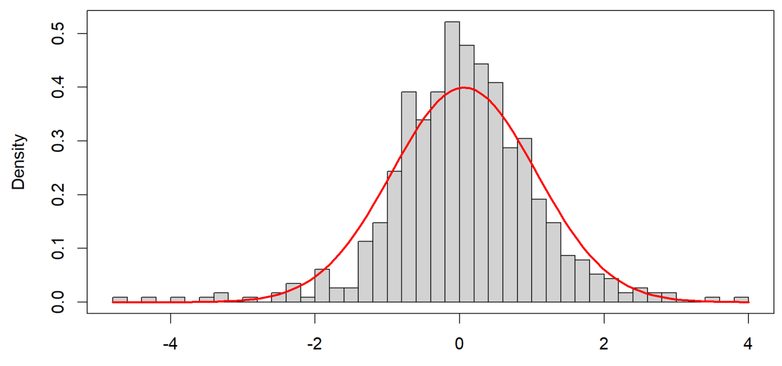
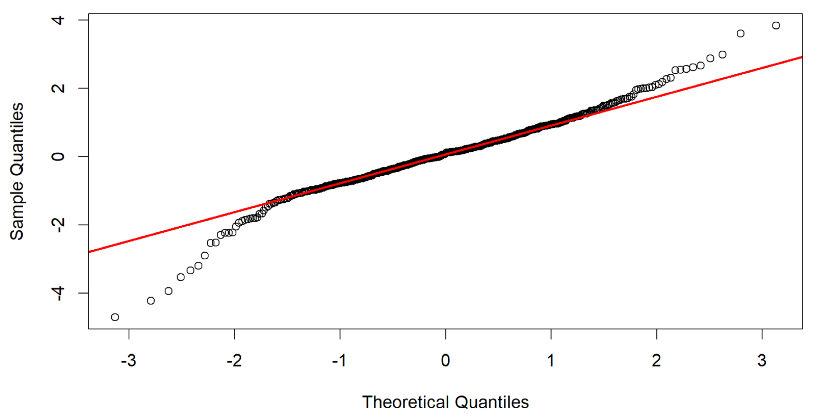
We start with the widely used Box–Jenkins methodology. Figure 1 displays the Australian carbon emissions futures prices spanning from 1 May 2011 to 1 May 2022 (for illustrative purposes). To identify any heavy tails, skewness, or deviations from symmetry within the distribution, a quantile–quantile (Q−Q) plot is commonly employed. Figure 2 presents the results of the Q−Q plot for the carbon price, revealing the distribution’s characteristics.

In this case, the Australian carbon emissions futures prices were modeled using a Box–Jenkins approach, leading to the development of a GARCH model. GARCH models, as depicted in Figure 1, capture the presence of heavy tails or volatility-related information in either or both tails. Additionally, Figure 1 and Figure 2 suggest that a Student’s t-distribution is suitable for modeling the residuals in this univariate dataset.

Determining a bivariate elliptical distribution using the Box–Jenkins methodology can be challenging since it primarily focuses on univariate analysis. However, when modeling an elliptical or skew-elliptical distribution, one can use the R software function gwer to identify a suitable bivariate regression methodology.

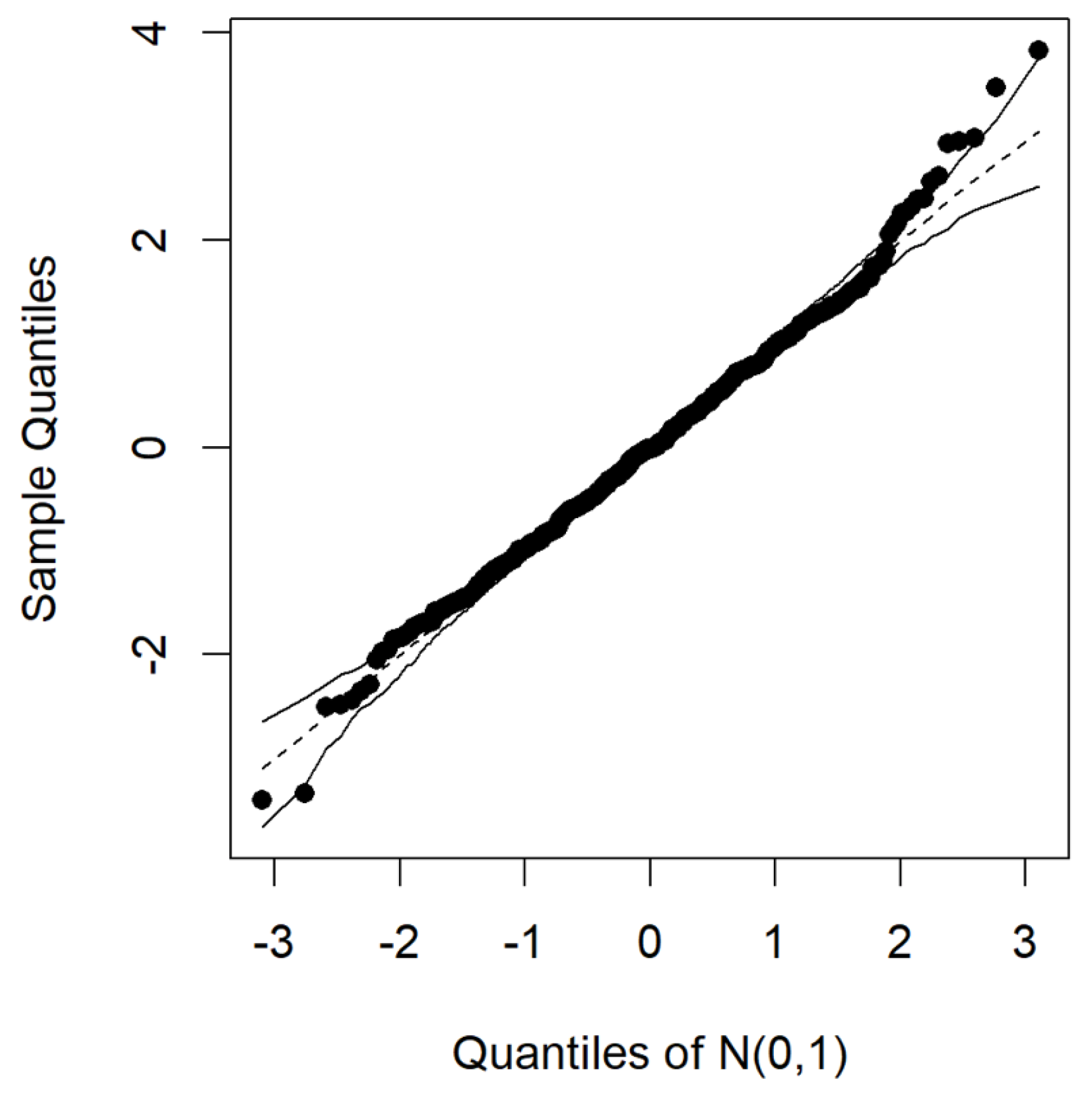
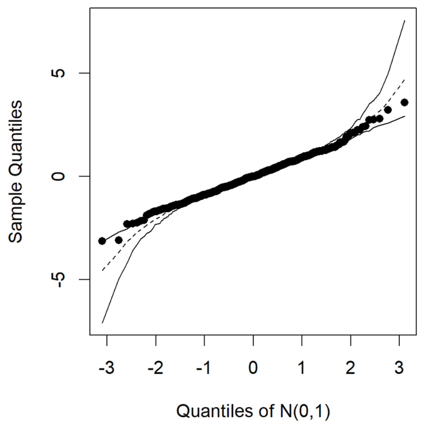
In this study, an elliptical regression model was applied to the Australian crude oil and natural gas weekly futures prices between 4 December 2012 and 28 November 2021. The resulting Q−Q residual plots are depicted in Figure 3 and Figure 4. These plots, along with the simulated envelope for the error distribution using elliptical regression, indicate that a symmetrical elliptical regression model would be appropriate. Most of the data points fall within or on the boundary line, particularly for the Student’s t-distribution.

To further aid in identifying a suitable regression modeling methodology (both elliptical and skew-elliptical), copula modeling can be utilized. Copula modeling allows for the identification of the underlying distribution, such as normal, Student’s t, Gumbel, BB1, and others, as described in Dewick and Liu (2022).

Given that elliptical and skew-elliptical distributions are composed of normal and/or Student’s t-distributions (symmetrical) as well as skew-elliptical distributions (asymmetrical), or mixtures of elliptical and skew-elliptical distributions, copula modeling provides valuable insights into the distribution characteristics.

When dealing with elliptical distributions, skew-elliptical distributions, or a combination of both, selecting an appropriate modeling strategy without prior knowledge of the distribution can be challenging. Determining suitable local influence diagnostics and regression methodologies that align with the modeled elliptical distribution can be cumbersome. However, copula modeling can aid in overcoming these challenges by providing valuable information about the distribution and guiding the modeling process.

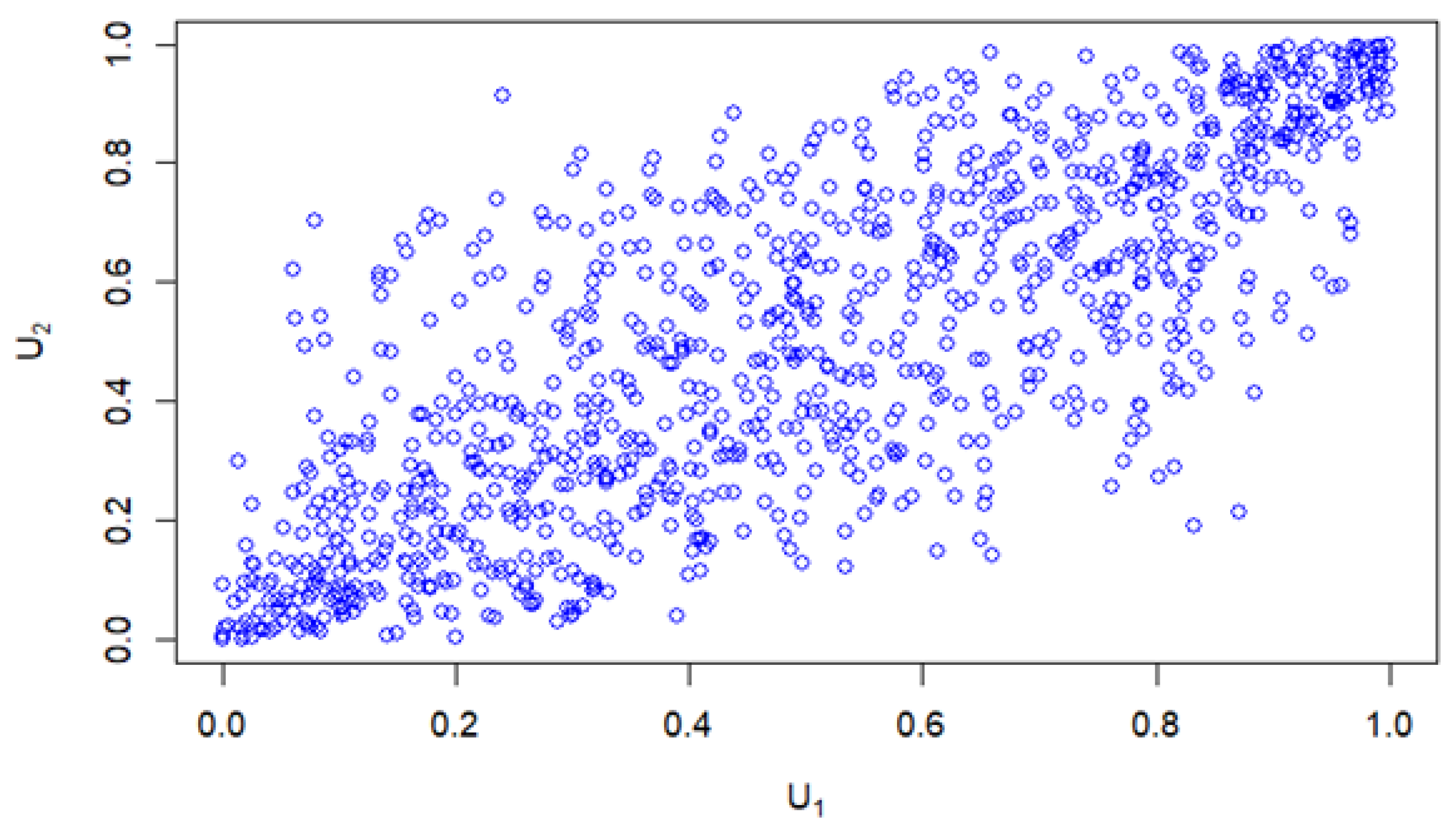
The identification of the copula distribution can help determine the appropriate regression modeling strategy, whether it is elliptical or skew-elliptical. The copula distribution provides insights into the dependency structure, as discussed by Kato et al. (2022). As an example, a normal copula distribution and copula forms have been simulated.

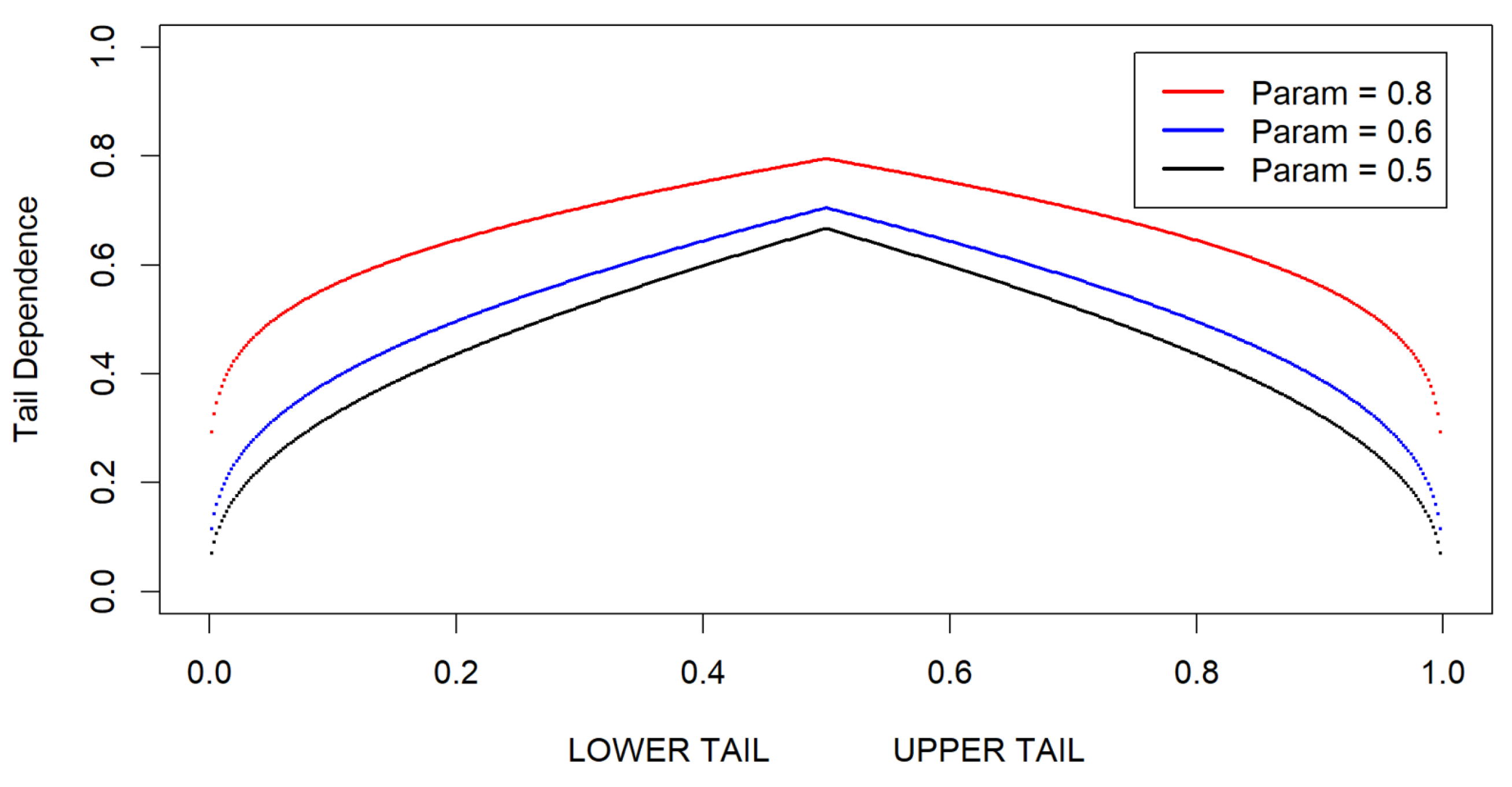
Figure 5 displays a normal copula distribution with a parameter value of 0.8. Additionally, Figure 6 presents examples of normal copula forms using parameter values of 0.8, 0.6, and 0.5. These copula distributions and forms exhibit symmetrical elliptical distribution patterns. Consequently, this highlights the suitability of elliptical local influence diagnostics and regression methods.

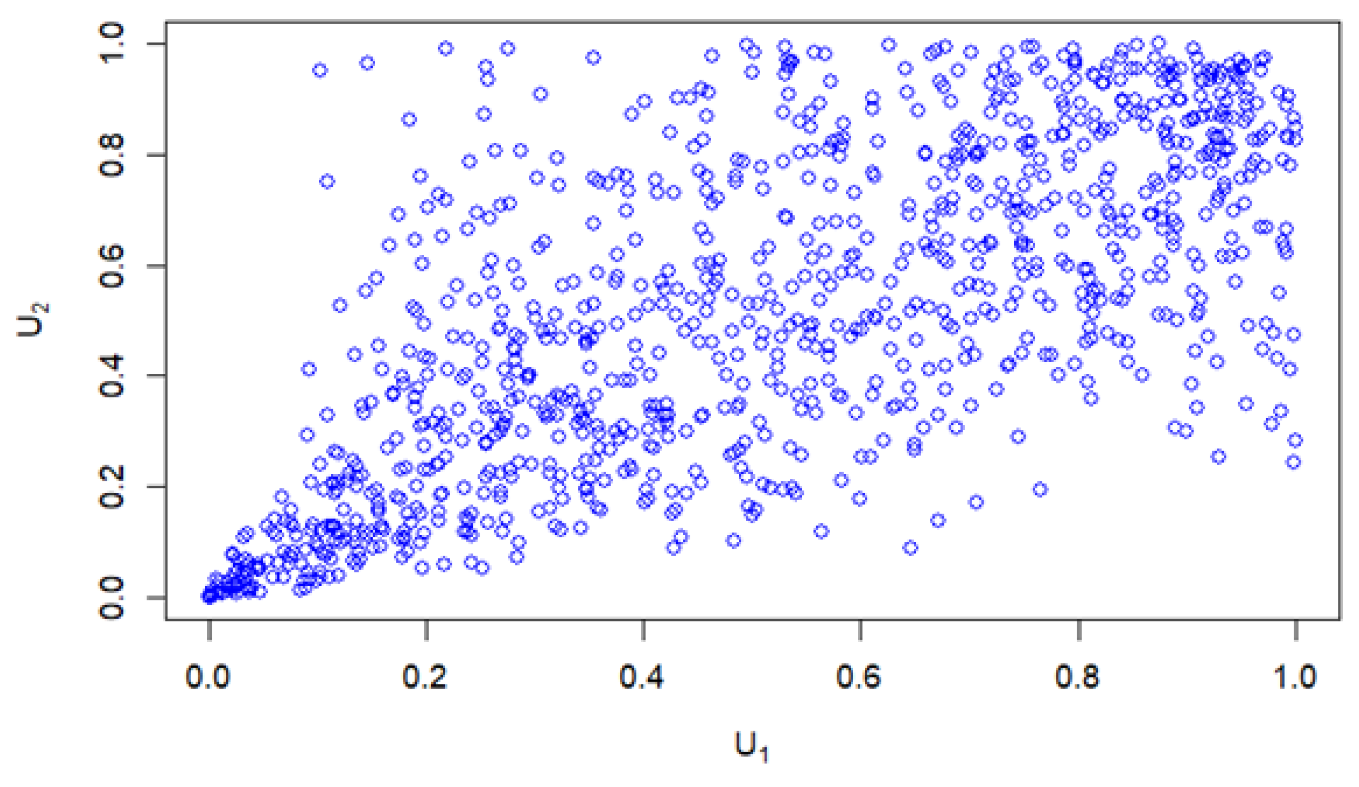
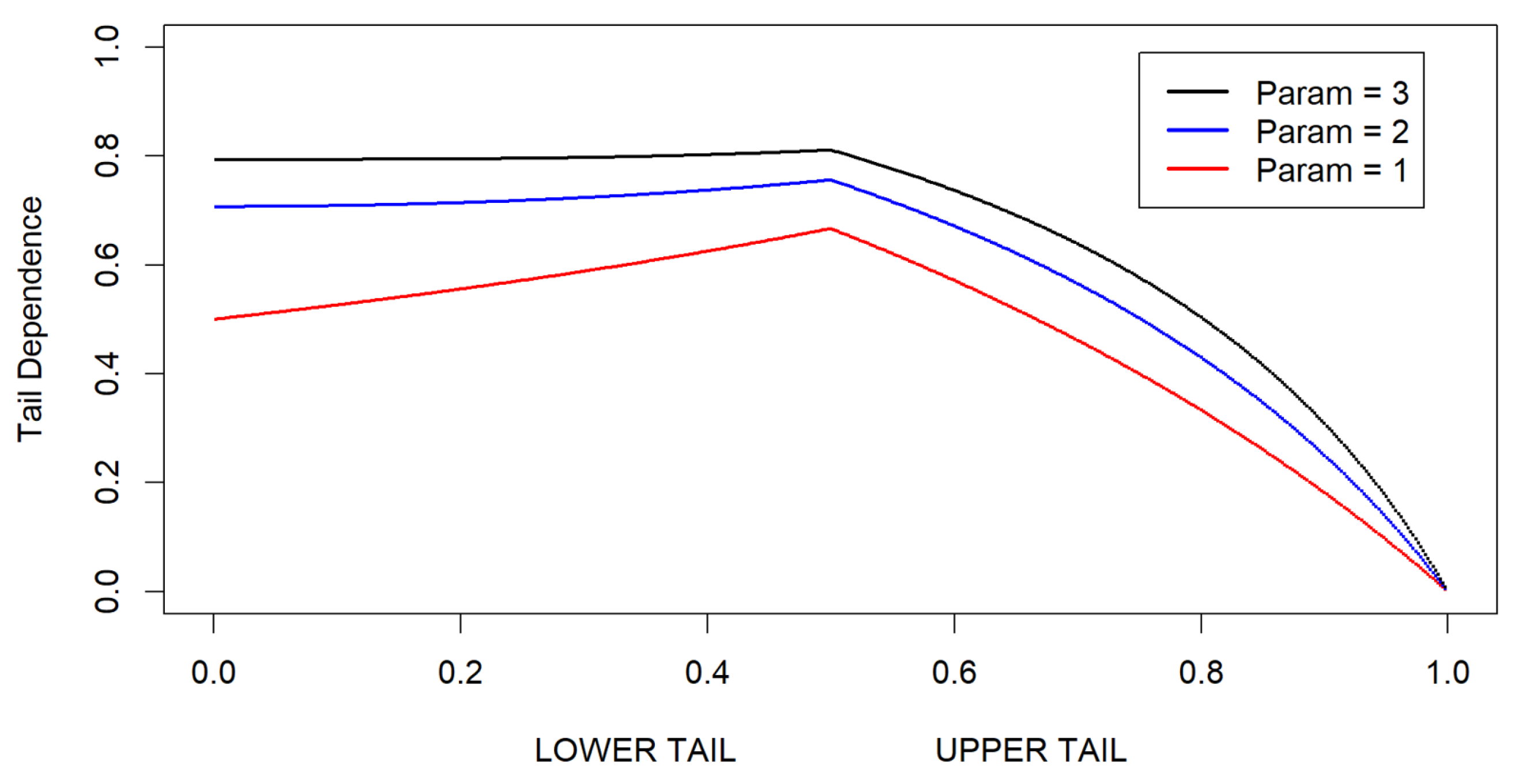
In another example, a simulated Clayton (Archimedean) copula distribution with its dependency structure is illustrated in Figure 7 and Figure 8. These figures emphasize the resulting skew-elliptical copula distributions. Figure 7 demonstrates a high concentration of data points in the lower-left region, while Figure 8 reveals the strong dependence within the lower tail of the copula. Such Archimedean-type copulas indicate the need for skew-elliptical local influence diagnostics and regression methods.

In real-world copula modeling scenarios, the selection of a copula model is advantageous as it allows for the modeling of the dependency structure in the data along with the chosen copula form, as indicated in Figure 9. However, it is important to note that the selected copula form may not fully capture the entire dependency structure of the modeled data, especially when there are issues with the marginal distributions’ uniformness.

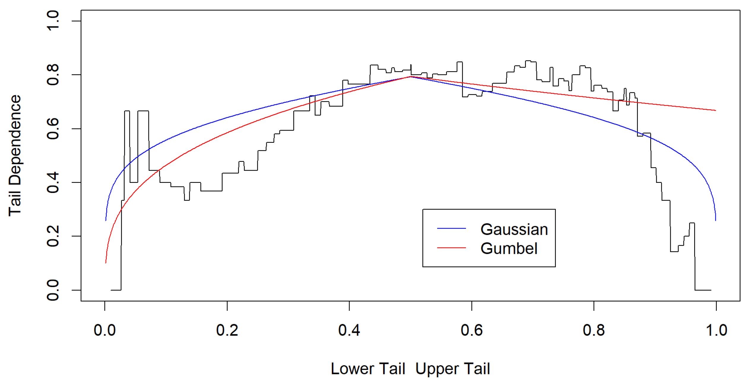
For example, the R base dataset “airquality” can be modeled using a copula approach with the variables “Ozone” and “Temperature”. Figure 9 illustrates the dependency structure obtained from this modeling process. It is evident from the figure that the chosen copula form is rigid and may have difficulties accurately representing the observed dependence structure. Nevertheless, the figure highlights a significant concentration of dependence in the upper-tail region, suggesting the suitability of a skew-elliptical regression model. Specifically, this dependence structure follows an (Archimedean) Gumbel distribution with a parameter value of 2.41.

When using the R software function BiCopSelect, the range of possible generated copulas is extensive. However, when it comes to copula regression, identifying a suitable copula model is challenging due to the limited range of available copula types. Dependence modeling helps in selecting the appropriate copula model, such as Gaussian, Clayton, or Gumbel. Figure 9 suggests the need for a regression technique that accommodates a skew-elliptical distribution.

8. Concluding Remarks

In this paper, we provided a comprehensive overview of elliptical and skew-elliptical regression modeling. We highlighted the importance of identifying the underlying elliptical or skew-elliptical distribution before engaging in local influence and regression modeling. The estimation methods for these two distributions differ, necessitating distinct modeling approaches. We examined the Box–Jenkins methodology as a means to identify the elliptical distribution. However, this univariate methodology may present challenges in the case of bivariate datasets. If the Box–Jenkins method yields two normal distributions, it suggests the suitability of an elliptical regression methodology. Conversely, if it produces two GARCH-type models, determining the resulting elliptical distribution becomes more complex without additional modeling methods.

To address this, we introduced copula modeling as a methodology for determining a bivariate elliptical or skew-elliptical distribution. Copula modeling has proven to be a viable option for identifying the underlying distribution, enabling local influence diagnostics and facilitating the selection of appropriate elliptical regression models. The findings of this paper have practical implications, as the accurate determination of the elliptical and skew-elliptical distribution supports the application of suitable local influence and regression methods. Moreover, it contributes to the fields of financial portfolio management, business, and insurance analytics, ensuring correct model specification.

In closing, we express our deep appreciation to the late Professor Chris Heyde. We deeply miss his presence, and we are grateful for his significant contributions to the advancement of financial modeling. His work continues to inspire and benefit not only us, his colleagues and students, but also the broader community engaged in financial modeling, both now and in the future.

References

- Adcock, Chris, and Adelchi Azzalini. 2020. A Selective Overview of Skew–Elliptical and Related Distributions and of their Applications. Symmetry 12: 118. [Google Scholar] [CrossRef] [Green Version]
- Arellano-Valle, Reinaldo B., and Adelchi Azzalini. 2013. The Centred Parameterization and Related Quantities of the Skew–t Distribution. Journal of Multivariate Analysis 113: 73–90. [Google Scholar] [CrossRef]
- Arellano-Vale, Reinaldo B., and Marc G. Genton. 2010. Multivariate Unified Skew–Elliptical Distributions. Chilean Journal of Statistics 1: 17–33. [Google Scholar]
- Azzalini, Adelchi. 2022. An Overview on the Progeny of the Skew–Normal Family—A Personal Perspective. Journal of Multivariate Analysis 188: 104851. [Google Scholar] [CrossRef]
- Azzalini, Adelchi, and Alessandra Dalla Valle. 1996. The Multivariate Skew–Normal Distribution. Biometrika 83: 715–26. [Google Scholar] [CrossRef]
- Azzalini, Adelchi, and Antonella Capitanio. 2013. The Skew–Normal and Related Families. Cambridge: Cambridge University Press, vol. 3. [Google Scholar]
- Bekaert, Geert, and Guojun Wu. 2000. Asymmetric Volatility and Risk in Equity Markets. The Review of Financial Studies 13: 1–42. [Google Scholar] [CrossRef] [Green Version]
- Bhatti, M. Ishaq, and Hung Quang Do. 2019. Recent Development In Copula And Its Applications To The Energy, Forestry And Environmental Sciences. International Journal of Hydrogen Energy 44: 19453–73. [Google Scholar] [CrossRef]
- Black, F. 1976. Studies of Stock Market Volatility Changes. In Proceedings of the American Statistical Association Business and Economic Statistics Section. Washington, DC: American Statistical Association. [Google Scholar]
- Branco, Marcia D., and Dipak K. Dey. 2002. Regression Model Under Skew Elliptical Error Distribution. Journal of Mathematical Sciences 1: 151–69. [Google Scholar]
- Campbell, Rachel A. J., Catherine S. Forbes, Kees G. Koedijk, and Paul Kofman. 2008. Increasing Correlations or Just Fat Tails? Journal of Empirical Finance 15: 287–309. [Google Scholar] [CrossRef]
- Campbell, Rachel, Kees Koedijk, and Paul Kofman. 2002. Increased Correlation in Bear Markets. Financial Analysts Journal 58: 87–94. [Google Scholar] [CrossRef]
- Cao, Linyu, Ruili Sun, Tiefeng Ma, and Conan Liu. 2023. On Asymmetric Correlations and Their Applications in Financial Markets. Journal of Risk and Financial Management 16: 187. [Google Scholar] [CrossRef]
- Cherubini, Umberto, Elisa Luciano, and Walter Vecchiato. 2004. Copula Methods in Finance. Hoboken: John Wiley & Sons. [Google Scholar]
- Christoffersen, Peter, Vihang Errunza, Kris Jacobs, and Hugues Langlois. 2012. Is the Potential for International Diversification Disappearing? A Dynamic Copula Approach. The Review of Financial Studies 25: 3711–51. [Google Scholar] [CrossRef] [Green Version]
- Cook, R. Dennis. 1986. Assessment of Local Influence. Journal of the Royal Statistical Society: Series B (Methodological) 48: 133–55. [Google Scholar]
- Dette, Holger, Ria Van Hecke, and Stanislav Volgushev. 2014. Some Comments on Copula–Based Regression. Journal of the American Statistical Association 109: 1319–24. [Google Scholar] [CrossRef]
- Dewick, Paul R. 2022. On Financial Distributions Modelling Methods: Application on Regression Models for Time Series. Journal of Risk and Financial Management 15: 461. [Google Scholar] [CrossRef]
- Dewick, Paul R., and Shuangzhe Liu. 2022. Copula Modelling to Analyse Financial Data. Journal of Risk and Financial Management 15: 104. [Google Scholar] [CrossRef]
- Dong, Hua, and Chuancun Yin. 2021. A Unified Treatment of Characteristic Functions of Symmetric Multivariate and Related Distributions. arXiv arXiv:2112.06472. [Google Scholar]
- Embrechts Paul, Filip Lindskog, and Alexander McNeil. 2001. Modelling dependence with copulas. Rapport technique, Département de mathématiques, Institut Fédéral de Technologie de Zurich, Zurich 14: 1–50. [Google Scholar]
- Fang, Kai-Tang, and Theodore W. Anderson. 1990. Statistical Inference in Elliptically Contoured and Related Distributions. New York: Allerton Press. [Google Scholar]
- Fang, Kai-Tang, and Yao-Ting Zhang. 1990. Generalized Multivariate Analysis. Beijing and Berlin: Science Press Beijing and Springer. [Google Scholar]
- Fernández, Carmen, and Mark F. J. Steel. 1999. Multivariate Student–t Regression Models: Pitfalls and Inference. Biometrika 86: 153–67. [Google Scholar] [CrossRef]
- Friendly, Michael, Georges Monette, and John Fox. 2013. Elliptical Insights: Understanding Statistical Methods Through Elliptical Geometry. Statistical Science 28: 1–39. [Google Scholar] [CrossRef]
- Fung, Thomas, and Eugene Seneta. 2021. Tail Asymptotics for the Bivariate Equi–skew Generalized Hyperbolic Distribution and its Variance–Gamma Special Case. Statistics & Probability Letters 178: 109182. [Google Scholar]
- Galea, Manuel, and Patricia Giménez. 2019. Local Influence Diagnostics for the Test of Mean–Variance Efficiency and Systematic Risks in the Capital Asset Pricing Model. Statistical Papers 60: 293–312. [Google Scholar] [CrossRef]
- Galea, Manuel, David Cademartori, Roberto Curci, and Alonso Molina. 2020. Robust inference in the capital asset pricing model using the multivariate t-distribution. Journal of Risk and Financial Management 6: 123. [Google Scholar] [CrossRef]
- Galea, Manuel P., Gilberto A. Paula, and Heleno Bolfarine. 1997. Local Influence in Elliptical Linear Regression Models. Journal of the Royal Statistical Society: Series D (The Statistician) 46: 71–79. [Google Scholar] [CrossRef]
- Galea, Manuel, Gilberto A. Paula, and Miguel Uribe-Opazo. 2003. On Influence Diagnostic in Univariate Elliptical Linear Regression Models. Statistical Papers 44: 23–45. [Google Scholar] [CrossRef]
- Galea, Manuel, Marco Riquelme, and Gilberto A. Paula. 2000. Diagnostic Methods in Elliptical Linear Regression Models. Brazilian Journal of Probability and Statistics 14: 167–84. [Google Scholar]
- Gani, Joseph M., and Eugene Seneta. 2004. Christopher Charles Heyde, AM, DSc, FAA, FAASA. Journal of Applied Probability, 41A (Special issue) 41: vii–x. [Google Scholar]
- Genton, Marc G. 2004. Skew-Elliptical Distributions and Their Applications: A Journey Beyond Normality. Boca Raton: CRC Press. [Google Scholar]
- Ghani, Intan M. Md., and Hanafi A. Rahim. 2019. Modeling and Forecasting of Volatility using ARMA–GARCH: Case Study on Malaysia Natural Rubber Prices. IOP Conference Series: Materials Science and Engineering 548: 012023. [Google Scholar] [CrossRef]
- Glasserman, Paul, and Steven Kou. 2006. A Conversation With Chris Heyde. Statistical Science 21: 286–98. [Google Scholar] [CrossRef] [Green Version]
- Gródek-Szostak, Zofia, Gabriela Malik, Danuta Kajrunajtys, Anna Szeląg-Sikora, Jakub Sikora, Maciej Kuboń, Marcin Niemiec, and Joanna Kapusta-Duch. 2019. Modeling The Dependency Between Extreme Prices Of Selected Agricultural Products On The Derivatives Market Using The Linkage Function. Sustainability 11: 4144. [Google Scholar] [CrossRef] [Green Version]
- Guan, Jing, Daoji Shi, and Yuanyuan He. 2008. Copula Quantile Regression and Measurement of Risk in Finance. Paper presented at 2008 4th International Conference on Wireless Communications, Networking and Mobile Computing, Dalian, China, October 12–14; pp. 1–4. [Google Scholar]
- Gupta, Arjun K., Tamas Varga, and Taras Bodnar. 2013. Elliptically Contoured Models in Statistics and Portfolio Theory. New York: Springer. [Google Scholar]
- Gupta, Neha, Arun Kumar, and Nikolai Leonenko. 2021. Stochastic Models with Mixtures of Tempered Stable Subordinators. Mathematical Communications 26: 77–99. [Google Scholar]
- Heyde, Christopher C. 1967. On the Influence of Moments on the Rate of Convergence to the Normal Distribution. Zeitschrift für Wahrscheinlichkeitstheorie und Verwandte Gebiete 8: 12–18. [Google Scholar] [CrossRef]
- Heyde, Christopher C. 1999. A Risky Asset Model with Strong Dependence through Fractal Activity Time. Journal of Applied Probability 36: 1234–39. [Google Scholar] [CrossRef]
- Heyde, Christopher C., and Nikolai N. Leonenko. 2005. Student Processes. Advances in Applied Probability 37: 342–65. [Google Scholar] [CrossRef] [Green Version]
- Heyde, Christopher C., and Shuangzhe Liu. 2001. Empirical Realities for a Minimal Description Risky Asset Model. The Need for Fractal Features. Journal of the Korean Mathematical Society 38: 1047–59. [Google Scholar]
- Heyde, Christopher C., Shuangzhe Liu, and Roger Gay. 2001. Fractal scaling and Black-Scholes: The Full Story. A New View of Long–Range Dependence in Stock Prices. JASSA 1: 29–32. [Google Scholar]
- Hofert, Marius, Ivan Kojadinovic, Martin Mächler, and Jun Yan. 2018. Elements of Copula Modeling with R. Cham: Springer Nature Switzerland. [Google Scholar]
- Joe, Harry. 2014. Dependence Modeling with Copulas. Boca Raton: CRC Press. [Google Scholar]
- Kariya, Takeaki, and Bimal K. Sinha. 1989. Robustness of Statistical Tests. Boca Raton: Academic Press. [Google Scholar]
- Kato, Shogo, Toshinao Yoshiba, and Shinto Eguchi. 2022. Copula-Based Measures of Asymmetry Between the Lower and Upper Tail Probabilities. Statistical Papers 63: 1907–29. [Google Scholar] [CrossRef]
- Kayalar, Derya E., C. Coşkun Küçüközmen, and A. Sevtap Selcuk-Kestel. 2017. The Impact of Crude Oil Prices on Financial Market Indicators: Copula Approach. Energy Economics 61: 162–73. [Google Scholar] [CrossRef]
- Kerss, Alexander D. J., Nikolai Leonenko, and Alla Sikorskii. 2014. Risky Asset Models with Tempered Stable Fractal Activity Time. Stochastic Analysis and Applications 32: 642–63. [Google Scholar] [CrossRef]
- Kwong, Hok S., and Saralees Nadarajah. 2022. A New Robust Class of Skew Elliptical Distributions. Methodology and Computing in Applied Probability 24: 1669–91. [Google Scholar] [CrossRef]
- Landsman, Zinoviy M., and Emiliano A. Valdez. 2003. Tail Conditional Expectations for Elliptical Distributions. North American Actuarial Journal 7: 55–71. [Google Scholar] [CrossRef] [Green Version]
- Lange, Kenneth L., Roderick J. A. Little, and Jeremy M. G. Taylor. 1989. Robust Statistical Modeling Using the t Distribution. Journal of the American Statistical Association 84: 881–96. [Google Scholar] [CrossRef] [Green Version]
- Lee, Sharon X., and Geoffrey J. McLachlan. 2013. On Mixtures of Skew Normal and Skew t–Distributions. Advances in Data Analysis and Classification 7: 241–66. [Google Scholar] [CrossRef] [Green Version]
- Lemonte, Artur J., and Alexandre G. Patriota. 2011. Multivariate Elliptical Models with General Parameterization. Statistical Methodology 8: 389–400. [Google Scholar] [CrossRef]
- Leonenko, Nikolai N., Stuart Petherick, and Alla Sikorskii. 2012. Fractal Activity Time Models for Risky Asset with Dependence and Generalized Hyperbolic Distributions. Stochastic Analysis and Applications 30: 476–92. [Google Scholar] [CrossRef]
- Li, Zhengxiao, Jan Beirlant, and Liang Yang. 2022. A New class of Copula Regression Models for Modelling Multivariate Heavy–Tailed Data. Insurance: Mathematics and Economics 104: 243–61. [Google Scholar] [CrossRef]
- Liu, Shuangzhe. 2000. On Local Influence for Elliptical Linear Models. Statistical Papers 41: 211–24. [Google Scholar] [CrossRef] [Green Version]
- Liu, Shuangzhe. 2002. Local Influence in Multivariate Elliptical Linear Regression Models. Linear Algebra and Its Applications 354: 159–74. [Google Scholar] [CrossRef] [Green Version]
- Liu, Shuangzhe. 2004. On Diagnostics in Conditionally Heteroskedastic Time Series Models under Elliptical Distributions. Journal of Applied Probability 41: 393–405. [Google Scholar] [CrossRef]
- Liu, Shuangzhe, and Christopher C. Heyde. 2008. On Estimation in Conditional Heteroskedastic Time Series Models under Non–Normal Distributions. Statistical Papers 49: 455–69. [Google Scholar] [CrossRef]
- Liu, Shuangzhe, and Milind Sathye, eds. 2021. Financial Statistics and Data Analytics. (A reprint of the Special Issue published in Journal of Risk and Financial Management). Basel: MDPI. [Google Scholar]
- Liu, Shuangzhe, Christopher C. Heyde, and Wing-Keung Wong. 2011. Moment Matrices in Conditional Heteroskedastic Models under Elliptical Distributions with Applications in AR–ARCH Models. Statistical Papers 52: 621–32. [Google Scholar] [CrossRef] [Green Version]
- Liu, Yonghui, Guocheng Ji, and Shuangzhe Liu. 2015. Influence Diagnostics in a Vector Autoregressive Model. Journal of Statistical Computation and Simulation 85: 2632–55. [Google Scholar] [CrossRef]
- Liu, Yonghui, Chaoxuan Mao, Victor Leiva, Shuangzhe Liu, and Waldemiro A. Silva Neto. 2022a. Asymmetric Autoregressive Models: Statistical Aspects and a Financial Application under COVID-19 Pandemic. Journal of Applied Statistics 49: 1323–347. [Google Scholar] [CrossRef] [PubMed]
- Liu, Yonghui, Guonhua Mao, Victor Leiva, Shuangzhe Liu, and Alejandra Tapia. 2020. Diagnostic Analytics for an Autoregressive Model Under the Skew–Normal Distribution. Mathematics 8: 693. [Google Scholar] [CrossRef]
- Liu, Yonghui, Jing Wang, Victor Leiva, Alejandra Tapia, Wei Tan, and Shuangzhe Liu. 2023. Robust Autoregressive Modeling and its Diagnostic Analytics with a COVID-19 Related Application. Journal of Applied Statistics, 1–26. [Google Scholar] [CrossRef]
- Liu, Yonghui, Jing Wang, Zhao Yao, Conan Liu, and Shuangzhe Liu. 2022b. Diagnostic Analytics for a GARCH Model Under Skew-Normal Distributions. Communications in Statistics-Simulation and Computation, 1–25. [Google Scholar] [CrossRef]
- Ma, Yanyuan, Marc G. Genton, and Anastasios A. Tsiatis. 2005. Locally Efficient Semiparametric Estimators for Generalized Skew-Elliptical Distributions. Journal of the American Statistical Association 100: 980–89. [Google Scholar] [CrossRef]
- Madan, Dilip B., and Wim Schoutens. 2020. Self-Similarity in Long-Horizon Returns. Mathematical Finance 30: 1368–391. [Google Scholar] [CrossRef]
- Maller, Ross, Ishwar Basawa, Peter Hall, and Eugene Seneta. 2010. Selected Works of C. C. Heyde. New York: Springer. [Google Scholar]
- Meerschaert, Mark M., and Alla Sikorskii. 2019. Stochastic Models for Fractional Calculus, 2nd ed. Berlin: De Gruyter. [Google Scholar]
- Najafi, Zeinolabedin, Karim Zare, Mohammad R. Mahmoudi, Soheil Shokri, and Amir Mosavi. 2022. Inference and Local Influence Assessment in a Multifactor Skew–Normal Linear Mixed Model. Mathematics 10: 2820. [Google Scholar] [CrossRef]
- Nelsen, Roger B. 2007. An Introduction to Copulas. New York: Springer. [Google Scholar]
- Noh, Hohsuk, Anouar El Ghouch, and Taoufik Bouezmarni. 2013. Copula-Based Regression Estimation and Inference. Journal of the American Statistical Association 108: 676–88. [Google Scholar] [CrossRef] [Green Version]
- Osorio, Felipe, Gilberto A. Paula, and Manuel Galea. 2007. Assessment of Local Influence in Elliptical Linear Models with Longitudinal Structure. Computational Statistics & Data Analysis 51: 4354–368. [Google Scholar]
- Parsa, Rahul A., and Stuart A. Klugman. 2011. Copula Regression. Variance Advancing and Science of Risk 5: 45–54. [Google Scholar]
- Patton, Andrew J. 2004. On the Out-of-Sample Importance of Skewness and Asymmetric Dependence for Asset Allocation. Journal of Financial Econometrics 1: 130–68. [Google Scholar] [CrossRef] [Green Version]
- Patton, Andrew J. 2006. Modelling Asymmetric Exchange Rate Dependence. International Economic Review 47: 527–56. [Google Scholar] [CrossRef] [Green Version]
- Schmidt, Thorsten. 2007. Coping with Copulas. Copulas—From Theory to Application in Finance 3: 1–34. [Google Scholar]
- Seneta, Eugene, and Joseph M. Gani. 2009. Christopher Charles Heyde 1939–2008. Historical Records of Australian Science 20: 67–90. [Google Scholar] [CrossRef]
- SenGupta, Ashis, and Barry C. Arnold. 2022. Directional Statistics for Innovative Applications: A Bicentennial Tribute to Florence Nightingale. Singapore: Springer Nature Singapore. [Google Scholar]
- Sklar, M. 1959. Fonctions de Repartition an Dimensions et Leurs Marges. Publications de l’Institut Statistique de l’Université de Paris 8: 229–31. [Google Scholar]
- Stamatatou, Nikoletta, Lampros Vasiliades, and Athanasios Loukas. 2018. Bivariate Flood Frequency Analysis using Copulas. Proceedings 2: 635. [Google Scholar]
- Sungur, Engin A. 2006. Some Observations on Copula Regression Functions. Communications in Statistics—Theory and Methods 34: 9–10. [Google Scholar] [CrossRef]
- Vuolo, Mike. 2017. Copula Models For Sociology: Measures of Dependence and Probabilities for Joint Distributions. Sociological Methods and Research 46: 604–48. [Google Scholar] [CrossRef]
- Welsh, Alan H., and Alice M. Richardson. 1997. 13 Approaches to the Robust Estimation of Mixed Models. Handbook of Statistics 15: 343–84. [Google Scholar]
- Wichitaksorn, Nuttanan, S. T. Boris Choy, and Richard Gerlach. 2014. A Generalized Class of Skew Distributions and Associated Robust Quantile Regression Models. Canadian Journal of Statistics 42: 579–96. [Google Scholar] [CrossRef]
- Zeller, Camila B., Victor H. Lachos, and Filidor E. Vilca-Labra. 2011. Local Influence Analysis for Regression Models with Scale Mixtures of Skew-Normal Distributions. Journal of Applied Statistics 38: 343–68. [Google Scholar] [CrossRef]
Figure 1.
Histogram for the carbon price GARCH model residuals.
Figure 2.
Q−Q Plot for the carbon price GARCH model residuals.
Figure 3.
Q−Q plot for the normal elliptical regression residuals.
Figure 4.
Q−Q Plot for the Student’s t elliptical regression residuals.
Figure 5.
Normal Distribution (Parameter = 0.8).
Figure 6.
Normal Copula Dependencies.
Figure 7.
Clayton distribution (Parameter = 2).
Figure 8.
Clayton copula dependencies.
Figure 9.
Ozone and temperature dependence structure.