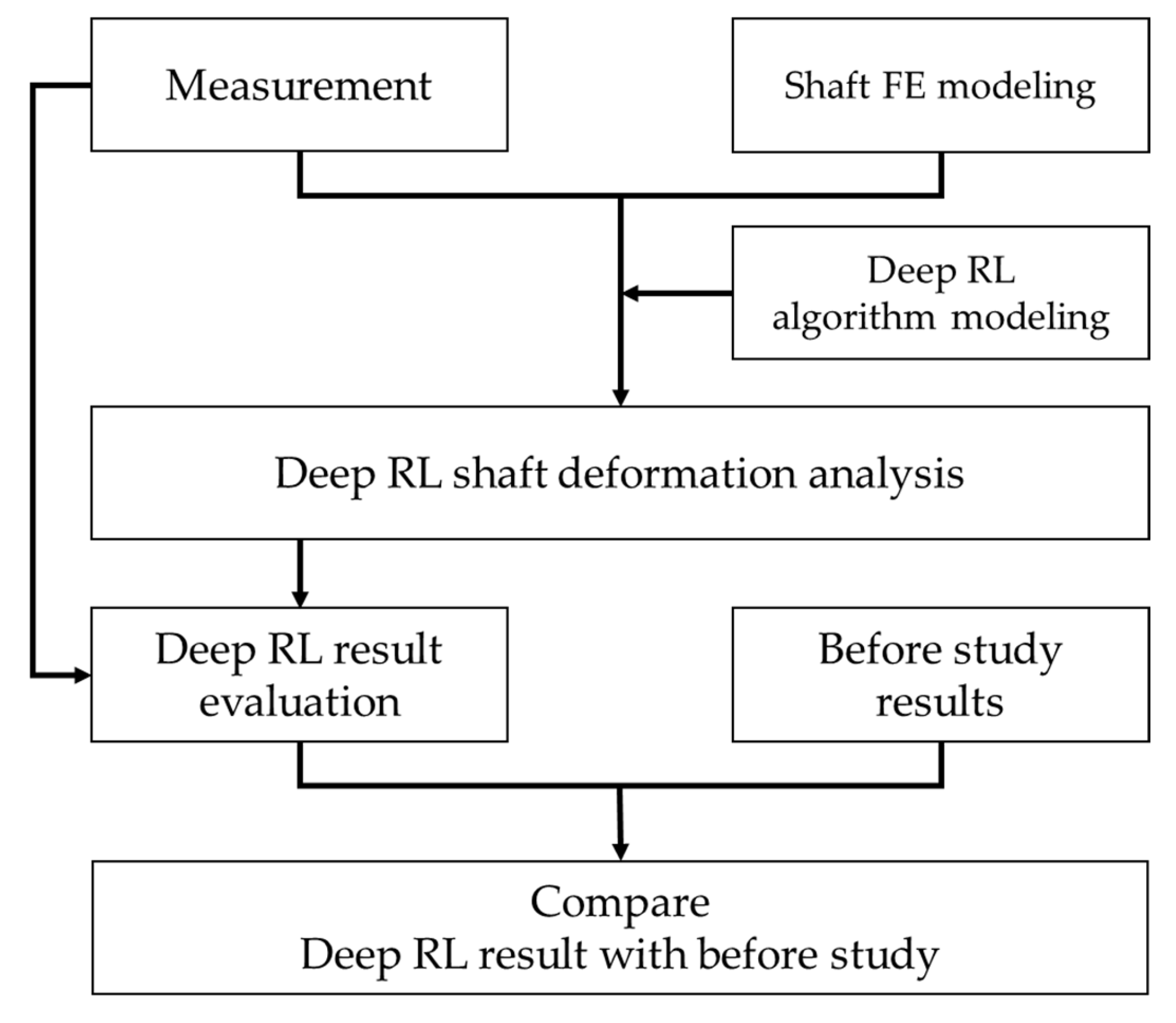
Figure 1.
Outline of study.
Figure 1.
Outline of study.
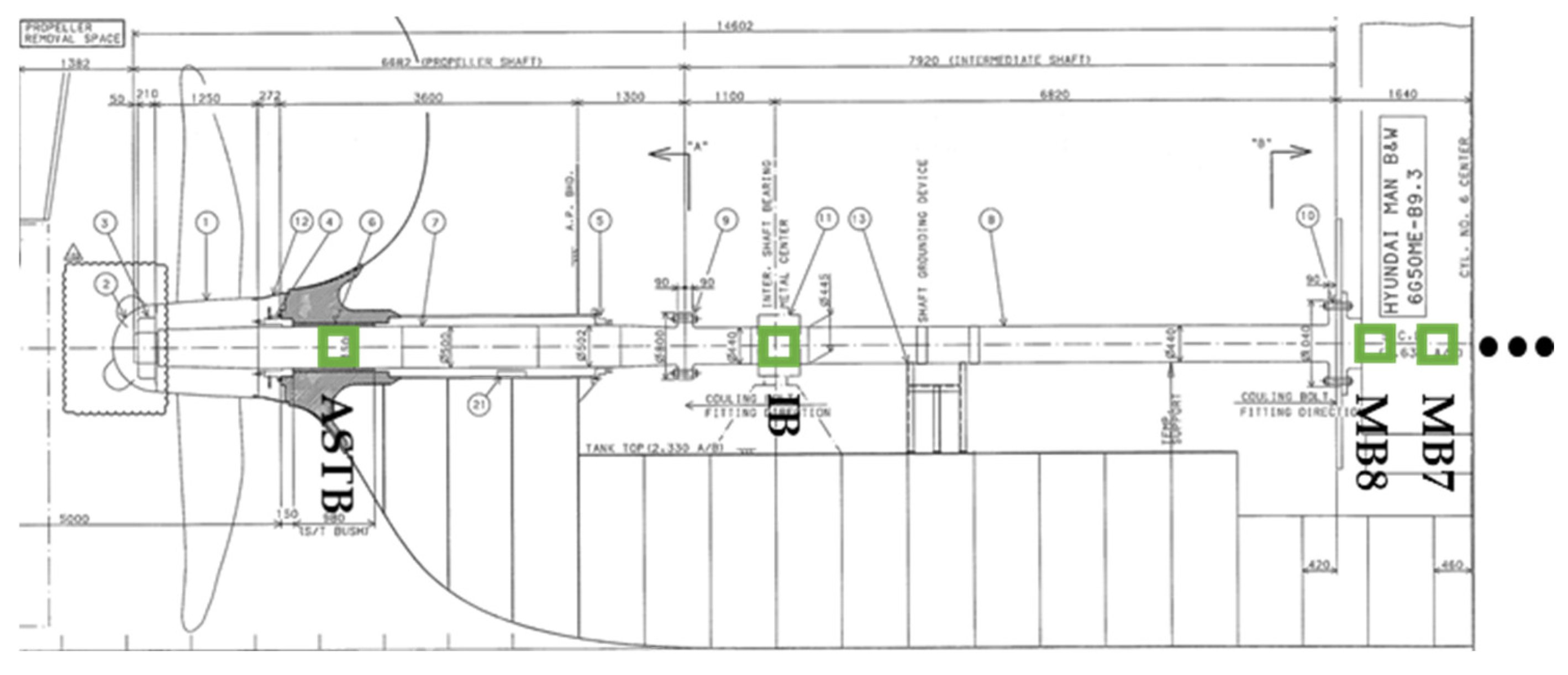
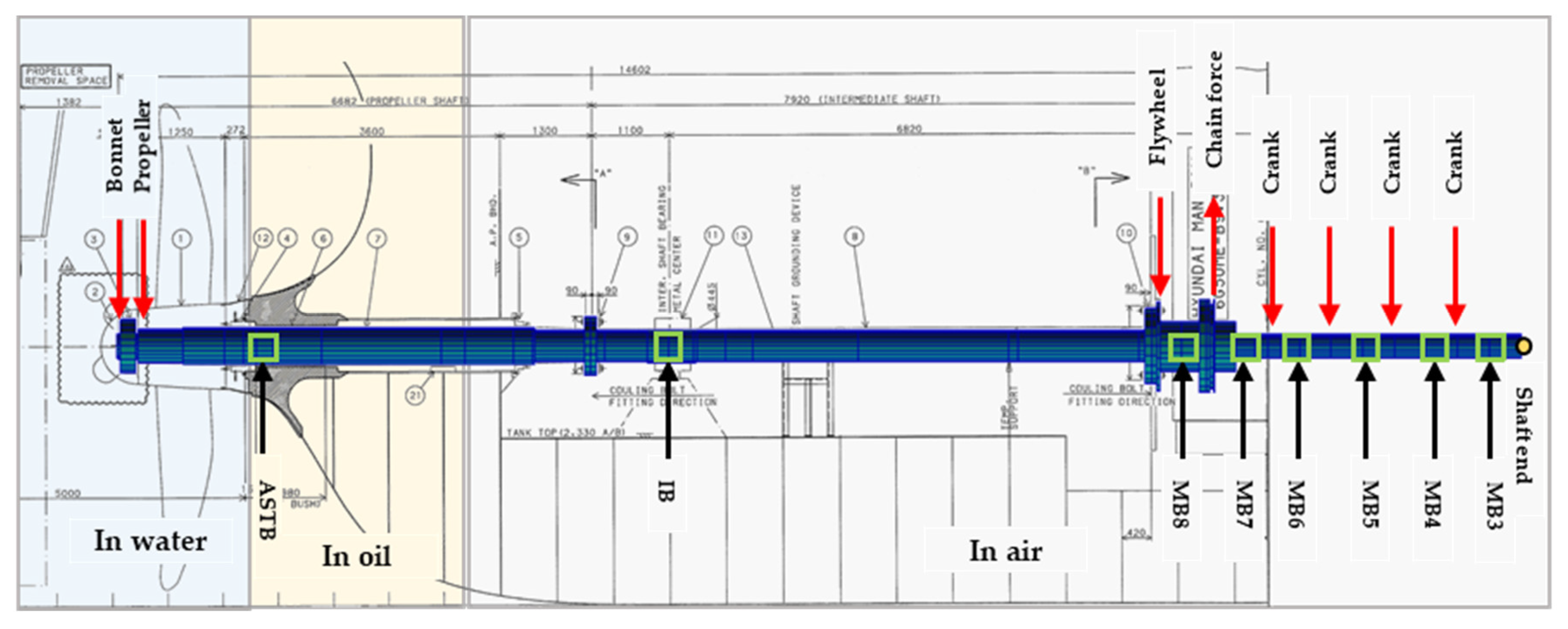
Figure 2.
Bearing positions of target ship.
Figure 2.
Bearing positions of target ship.
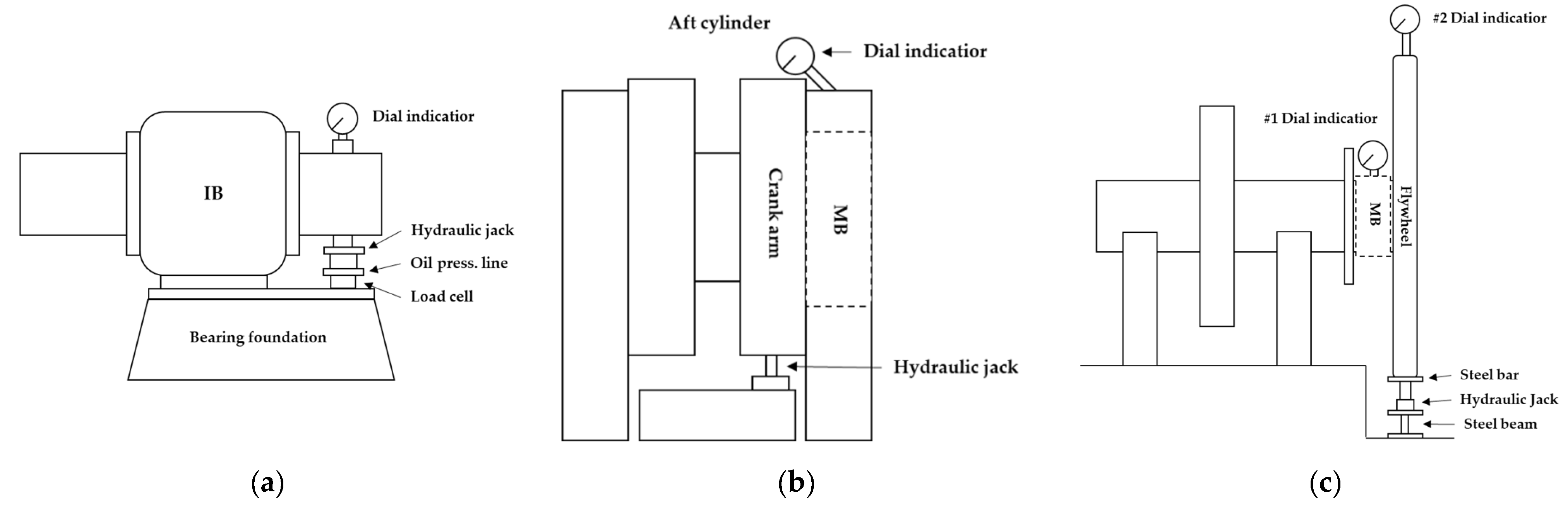
Figure 3.
Measurement using jack-up method: (a) intermediate bearing (IB), (b) main bearings (MBs) excluding aftmost MB, and (c) aftmost MB.
Figure 3.
Measurement using jack-up method: (a) intermediate bearing (IB), (b) main bearings (MBs) excluding aftmost MB, and (c) aftmost MB.
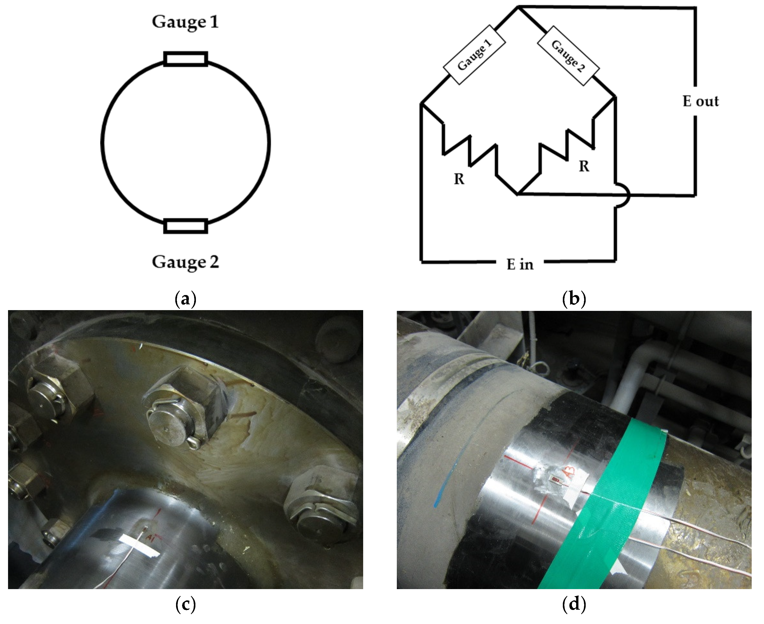
Figure 4.
(a) Wheatstone bridge connection method, (b) strain gauge attachment locations, and (c,d) strain gauge attachment examples.
Figure 4.
(a) Wheatstone bridge connection method, (b) strain gauge attachment locations, and (c,d) strain gauge attachment examples.
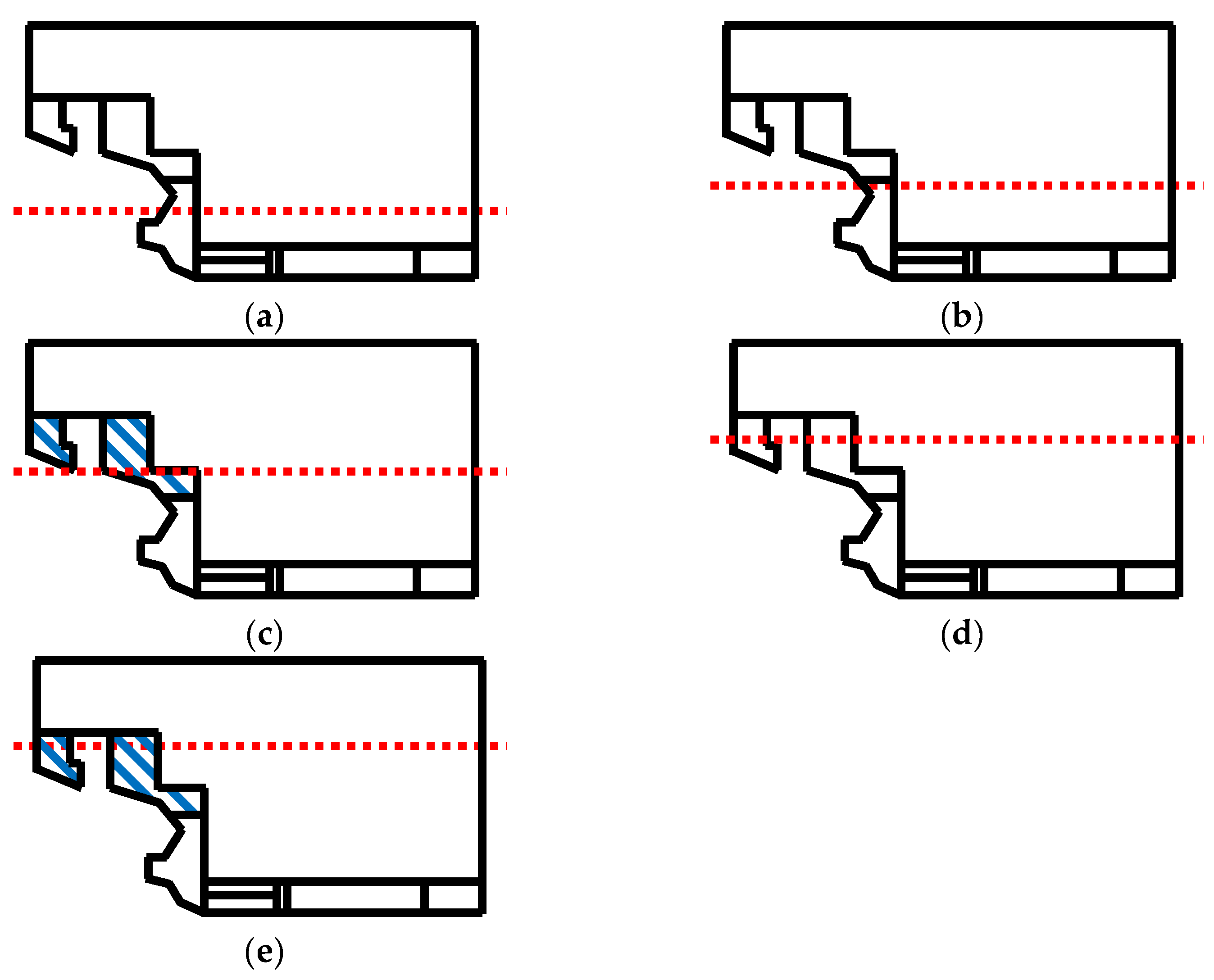
Figure 5.
Stern draft according to measurement draft conditions: (a) D1, (b) D2, (c) D3, (d) D4, and (e) D5.
Figure 5.
Stern draft according to measurement draft conditions: (a) D1, (b) D2, (c) D3, (d) D4, and (e) D5.
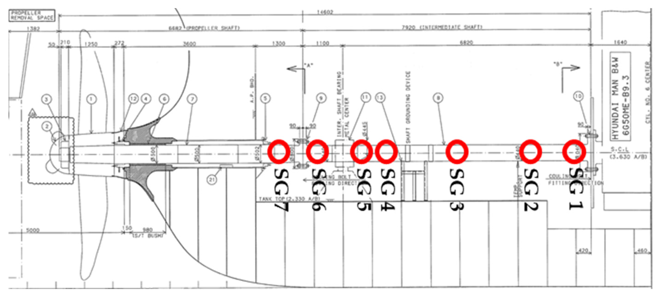
Figure 6.
Strain gauge attachment locations.
Figure 6.
Strain gauge attachment locations.
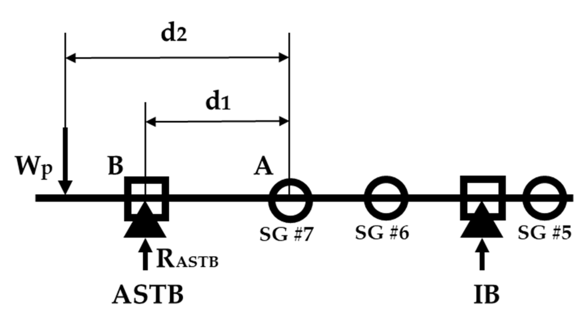
Figure 7.
ASTB moment equilibrium equation.
Figure 7.
ASTB moment equilibrium equation.
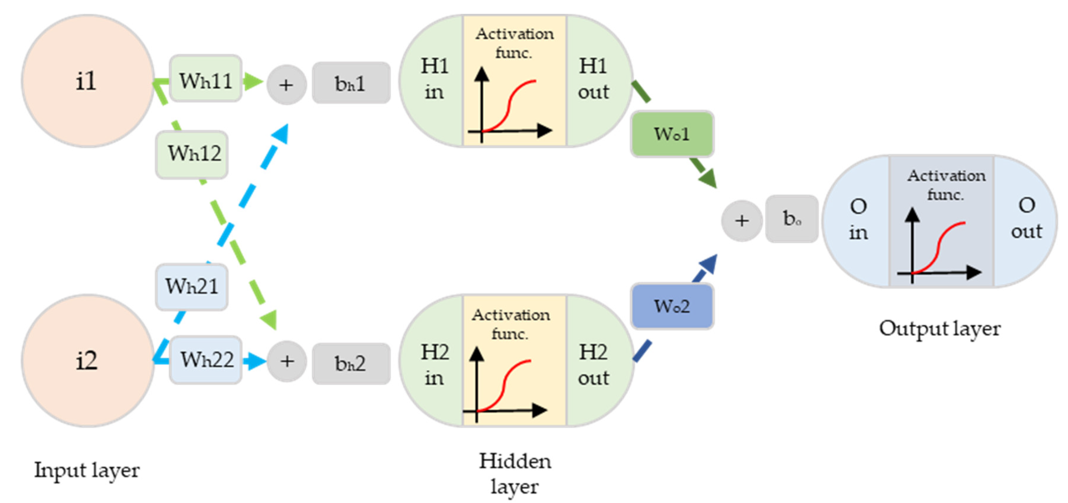
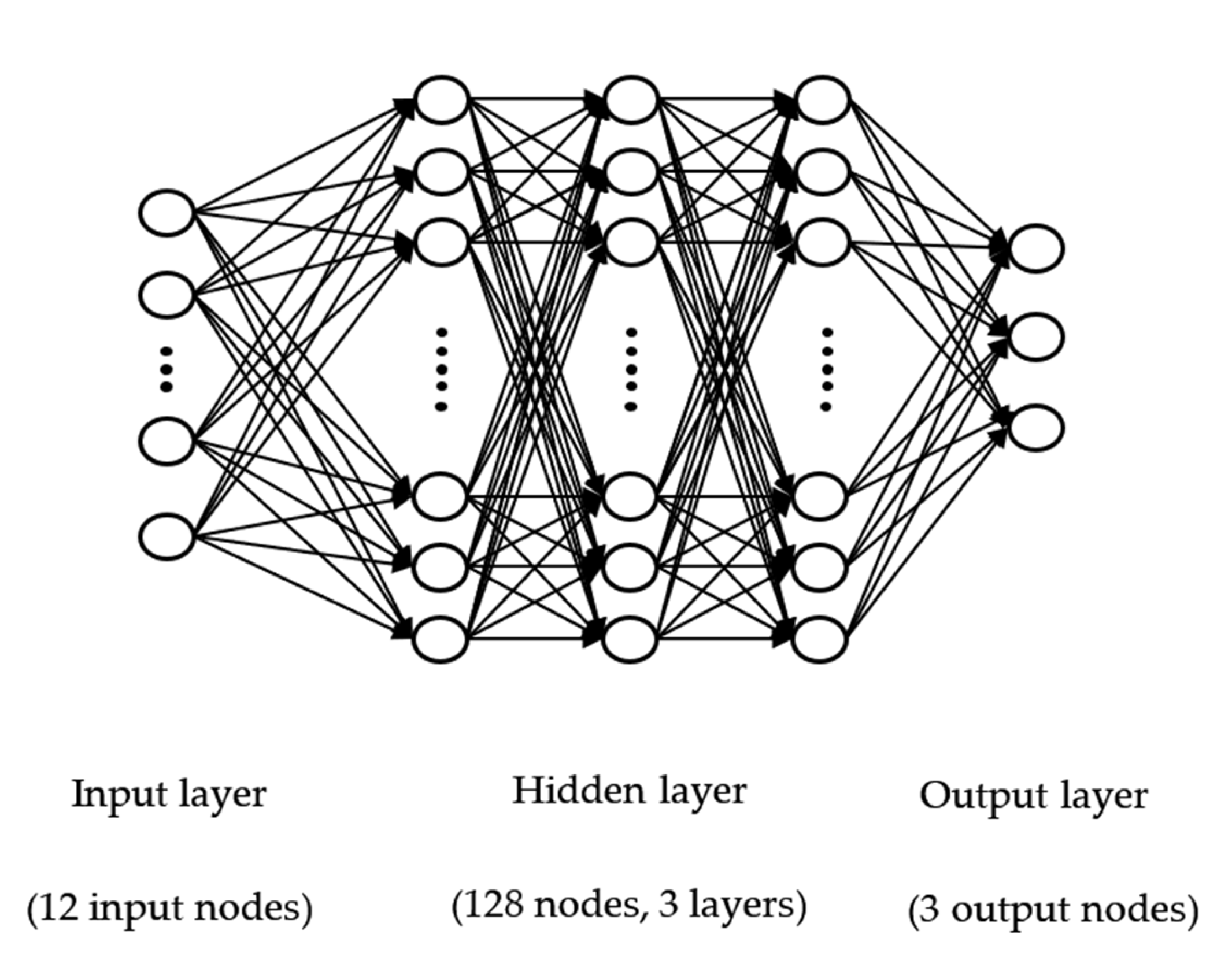
Figure 8.
Schematic of artificial neural network.
Figure 8.
Schematic of artificial neural network.
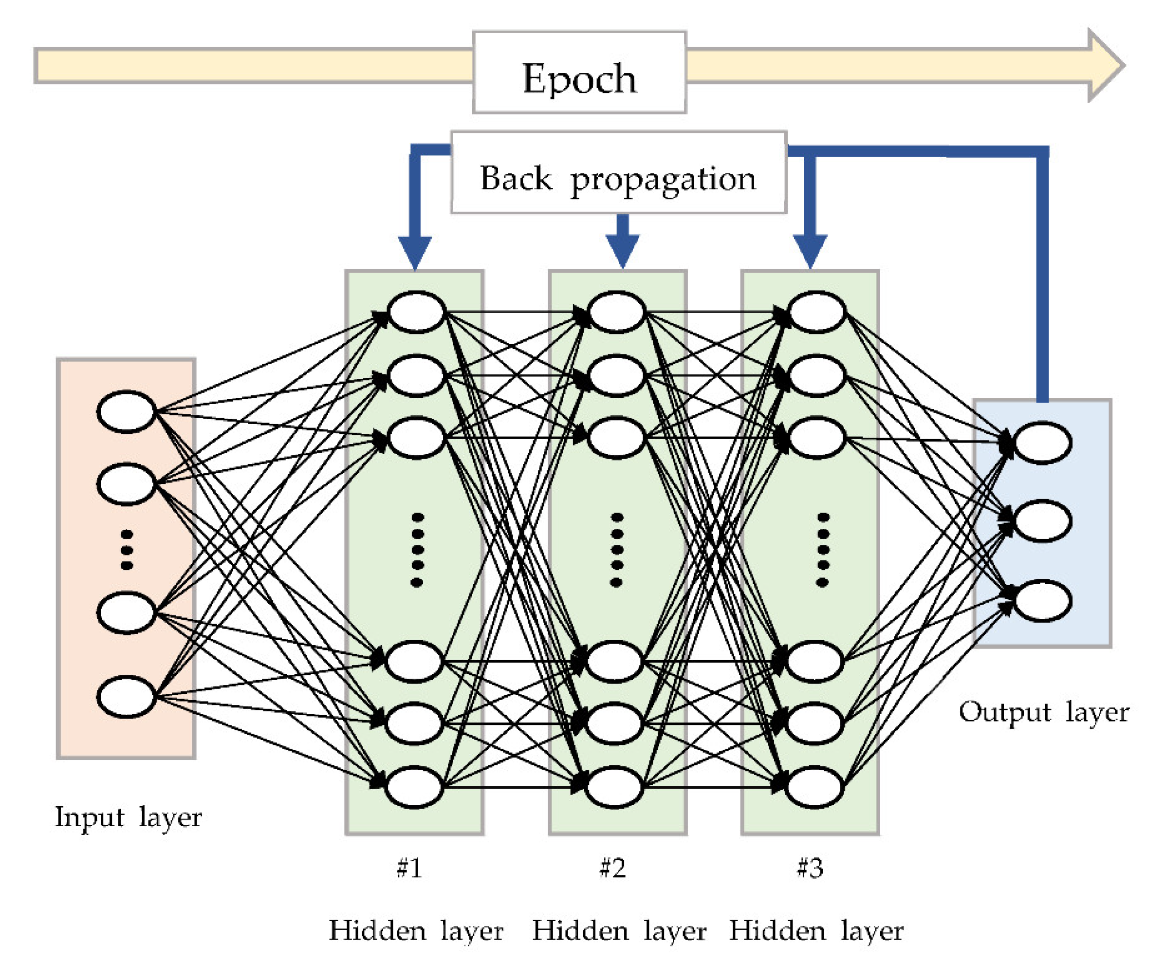
Figure 9.
Schematic of deep neural network.
Figure 9.
Schematic of deep neural network.
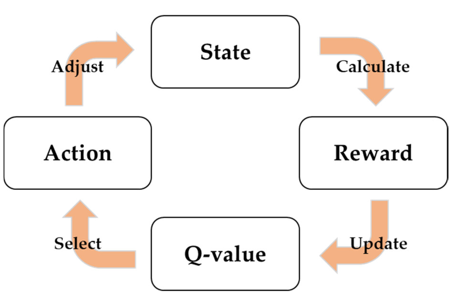
Figure 10.
Schematic of Q-learning [
26].
Figure 10.
Schematic of Q-learning [
26].
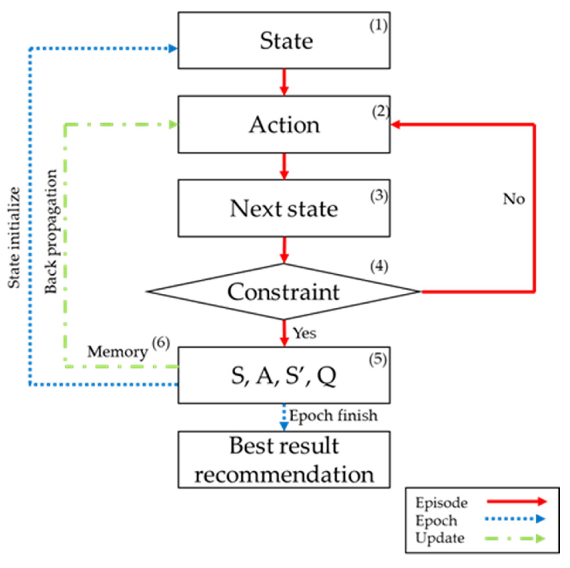
Figure 11.
Deep RL algorithm procedure.
Figure 11.
Deep RL algorithm procedure.
Figure 12.
Shaft FE model.
Figure 12.
Shaft FE model.
Figure 13.
Action decision deep neural network.
Figure 13.
Action decision deep neural network.
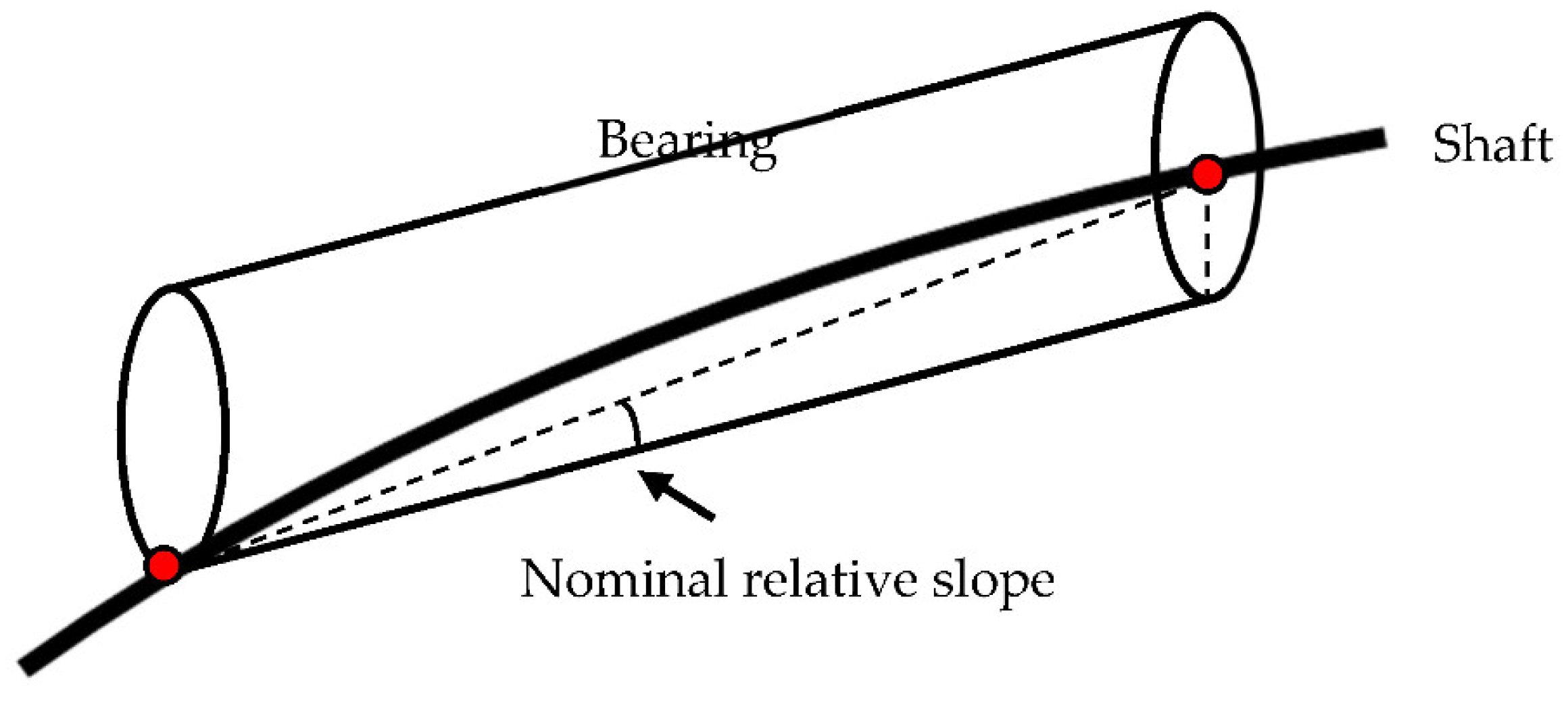
Figure 14.
Stern tube bearing relative slope angle.
Figure 14.
Stern tube bearing relative slope angle.
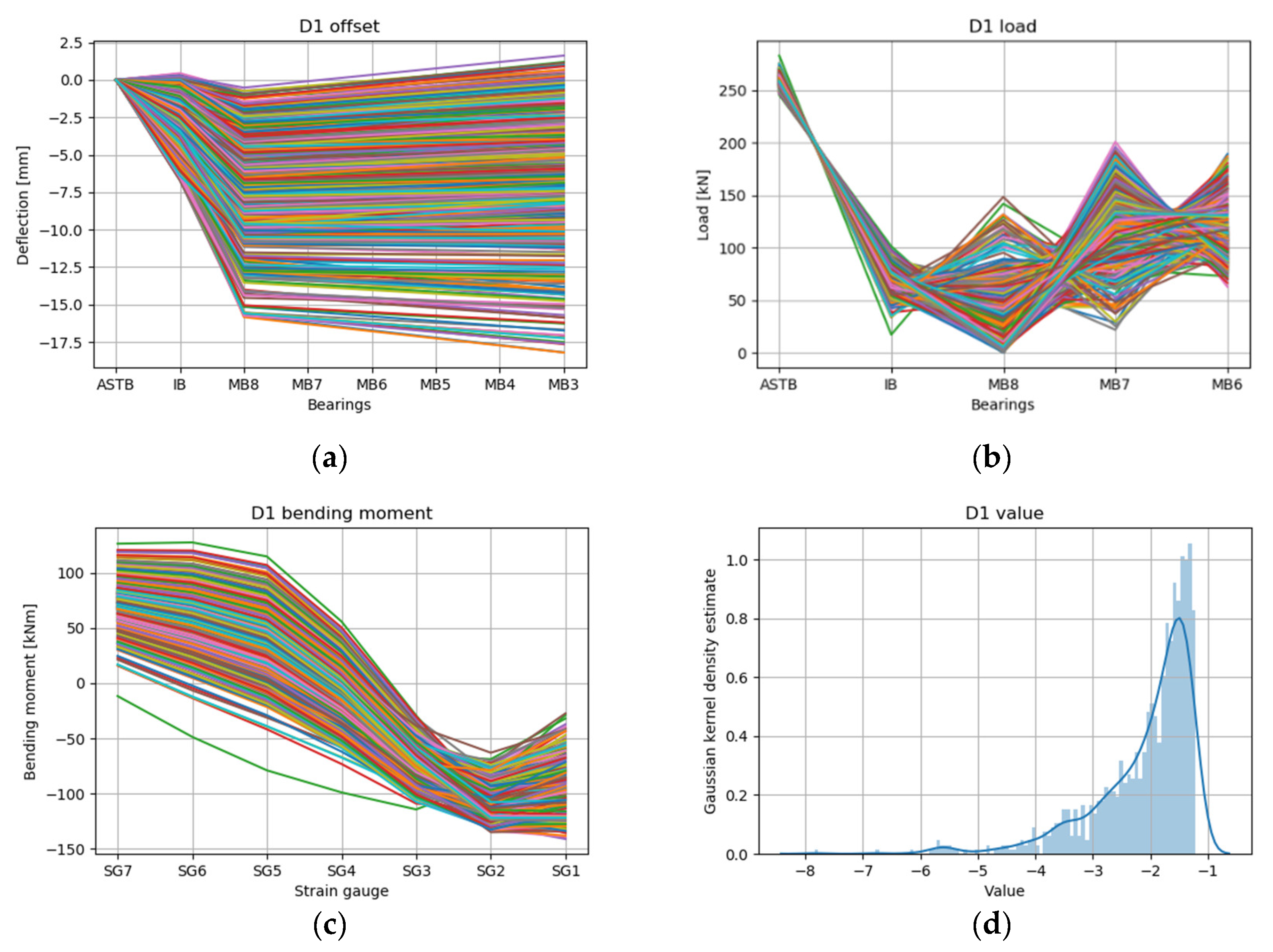
Figure 15.
RL results for draft condition D1 all cases: (a) offset, (b) load, (c) bending moment, and (d) value.
Figure 15.
RL results for draft condition D1 all cases: (a) offset, (b) load, (c) bending moment, and (d) value.
Figure 16.
RL results for draft condition D1 top 100 cases: (a) offset, (b) load, (c) bending moment, and (d) value.
Figure 16.
RL results for draft condition D1 top 100 cases: (a) offset, (b) load, (c) bending moment, and (d) value.
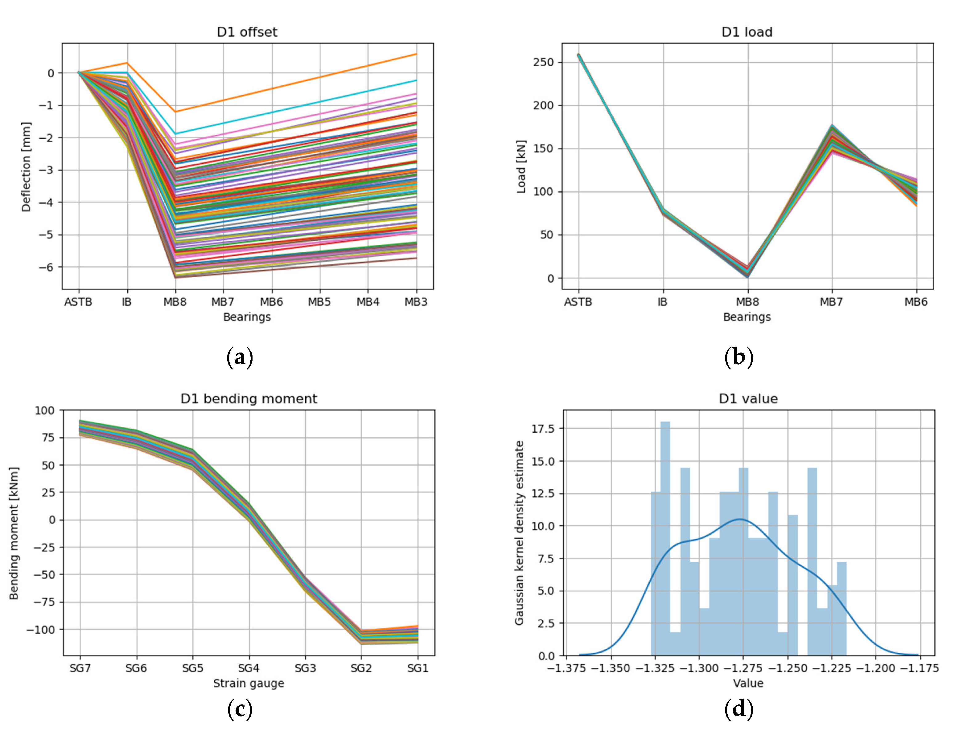
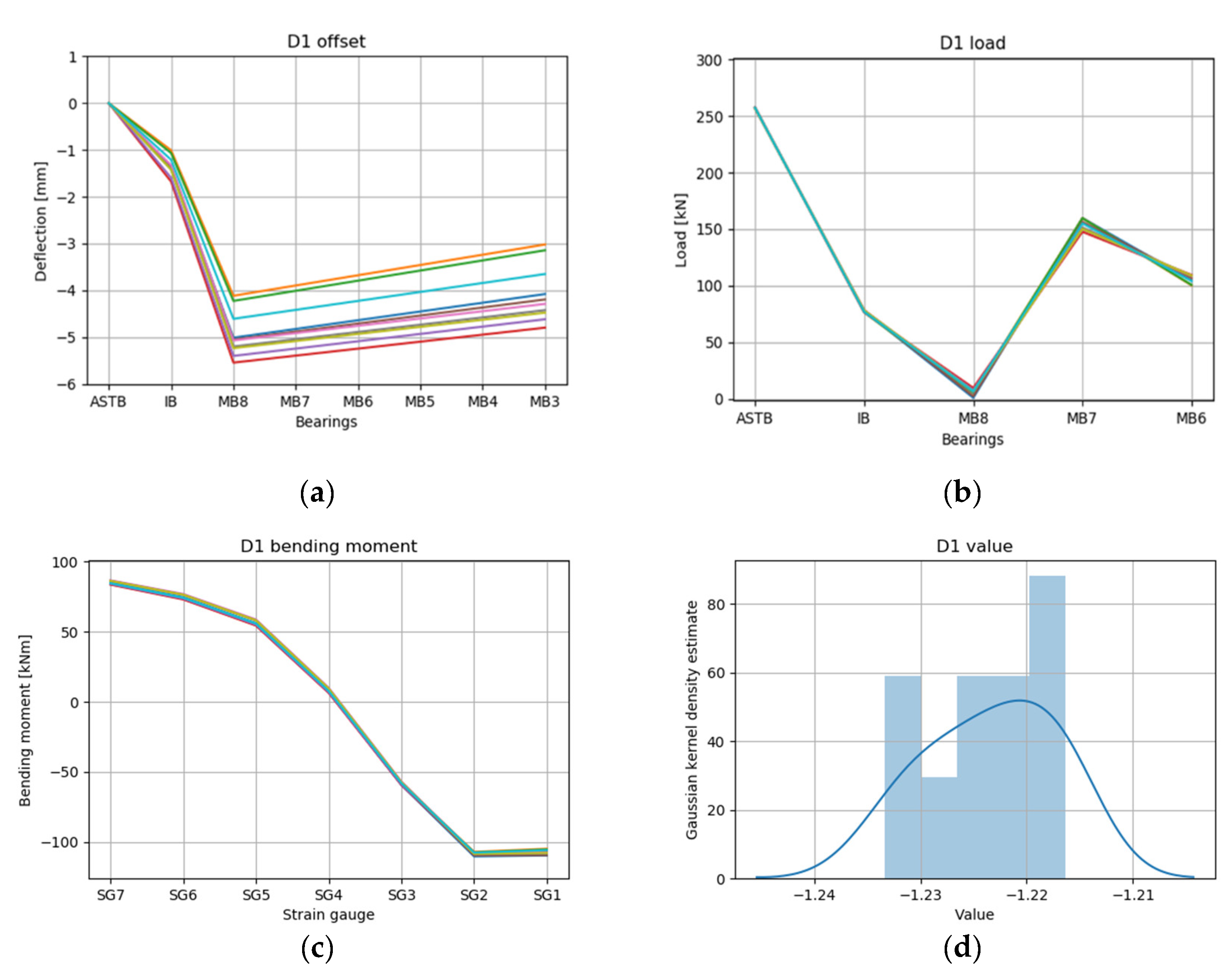
Figure 17.
RL results for draft condition D1 top 10 cases: (a) offset, (b) load, (c) bending moment, and (d) value.
Figure 17.
RL results for draft condition D1 top 10 cases: (a) offset, (b) load, (c) bending moment, and (d) value.
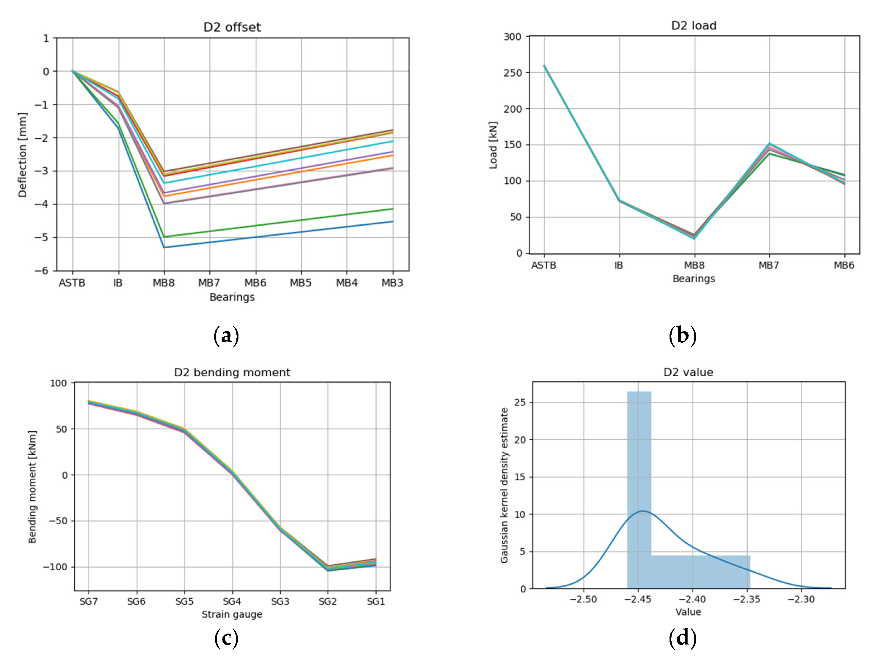
Figure 18.
RL results for draft condition D2 top 10 cases: (a) offset, (b) load, (c) bending moment, and (d) value.
Figure 18.
RL results for draft condition D2 top 10 cases: (a) offset, (b) load, (c) bending moment, and (d) value.
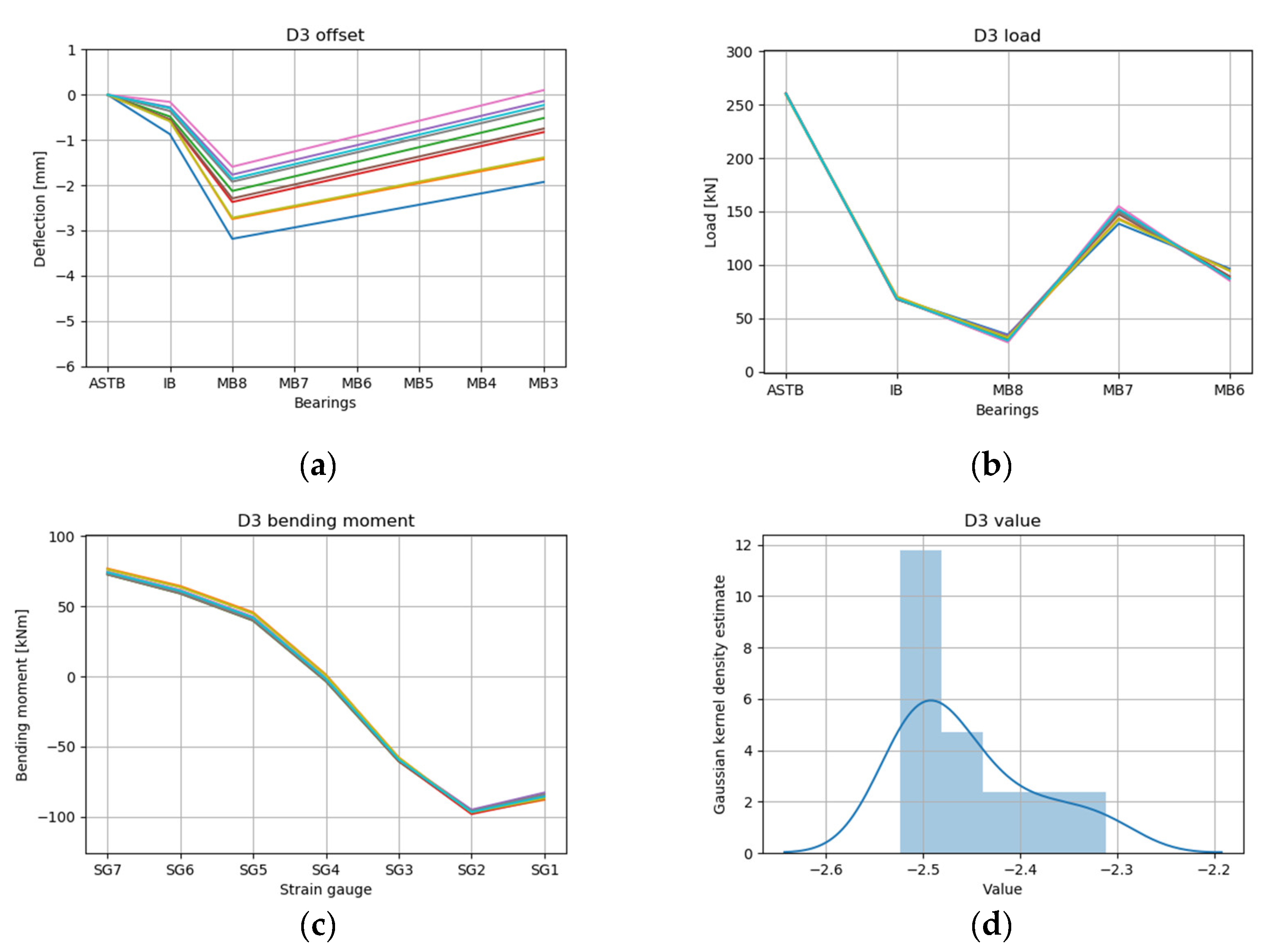
Figure 19.
RL results for draft condition D3 top 10 cases: (a) offset, (b) load, (c) bending moment, and (d) value.
Figure 19.
RL results for draft condition D3 top 10 cases: (a) offset, (b) load, (c) bending moment, and (d) value.
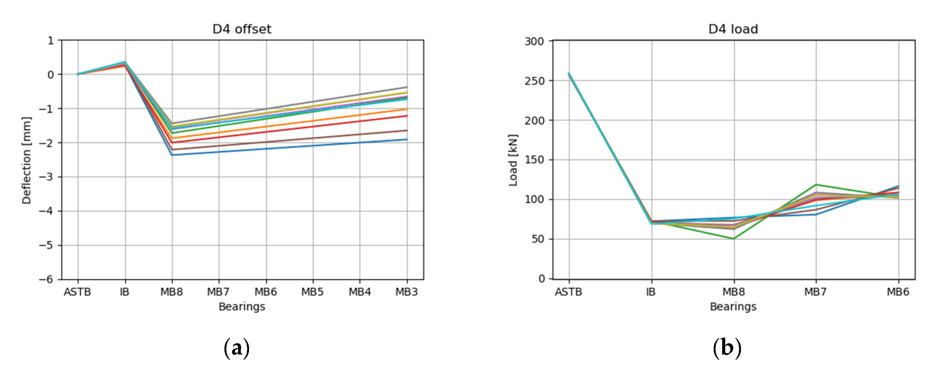
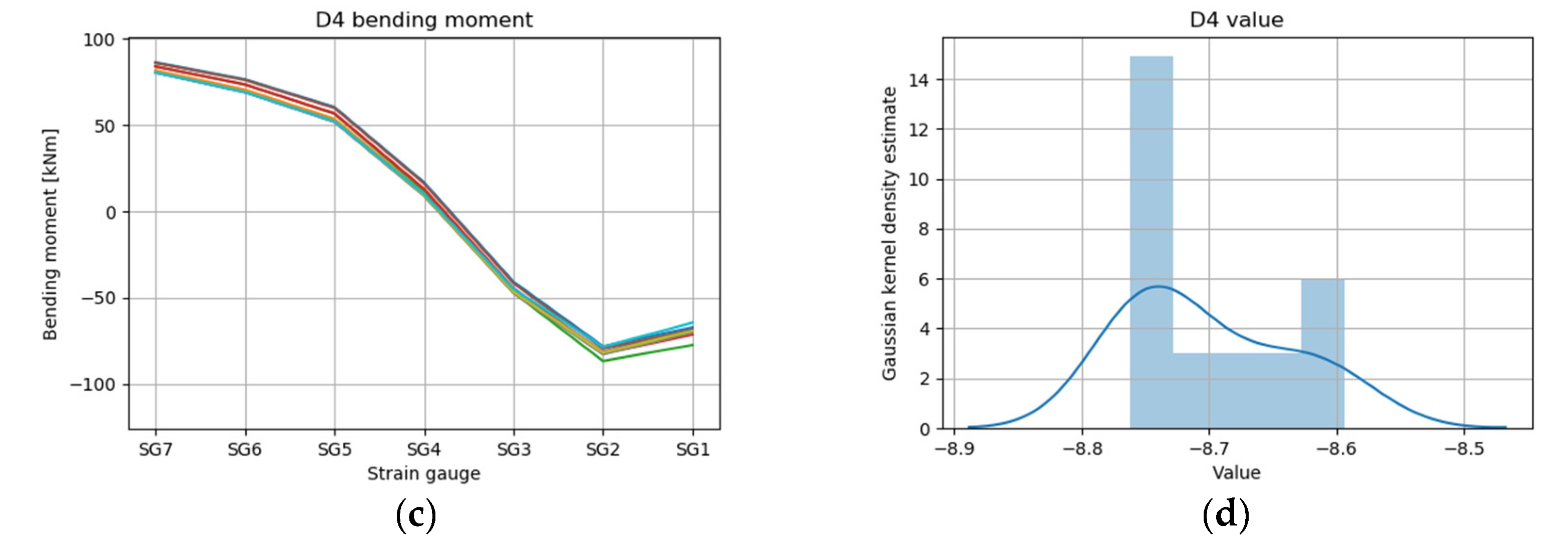
Figure 20.
RL results for draft condition D4 top 10 cases: (a) offset, (b) load, (c) bending moment, and (d) value.
Figure 20.
RL results for draft condition D4 top 10 cases: (a) offset, (b) load, (c) bending moment, and (d) value.
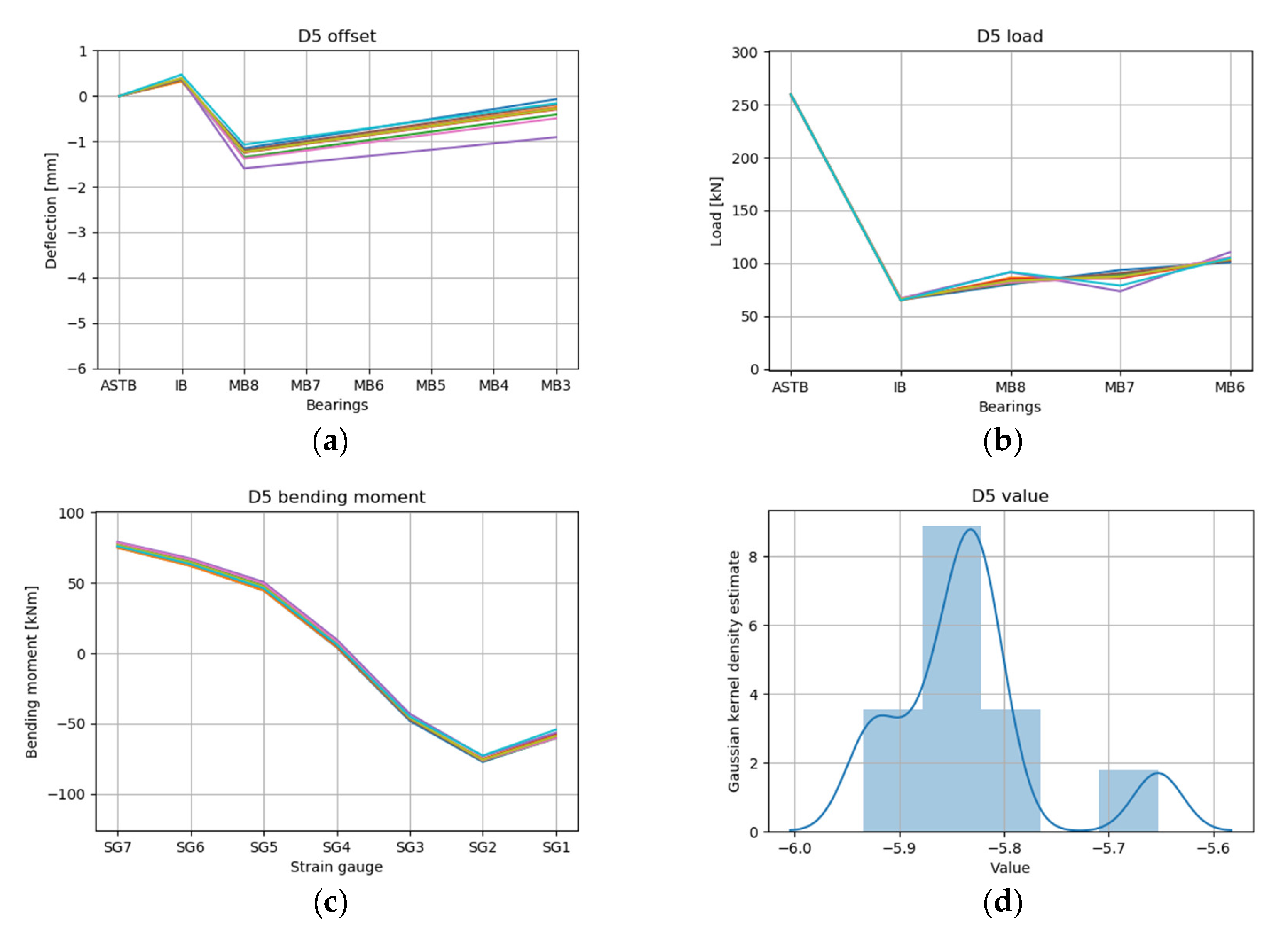
Figure 21.
RL results for draft condition D5 top 10 cases: (a) offset, (b) load, (c) bending moment, and (d) value.
Figure 21.
RL results for draft condition D5 top 10 cases: (a) offset, (b) load, (c) bending moment, and (d) value.
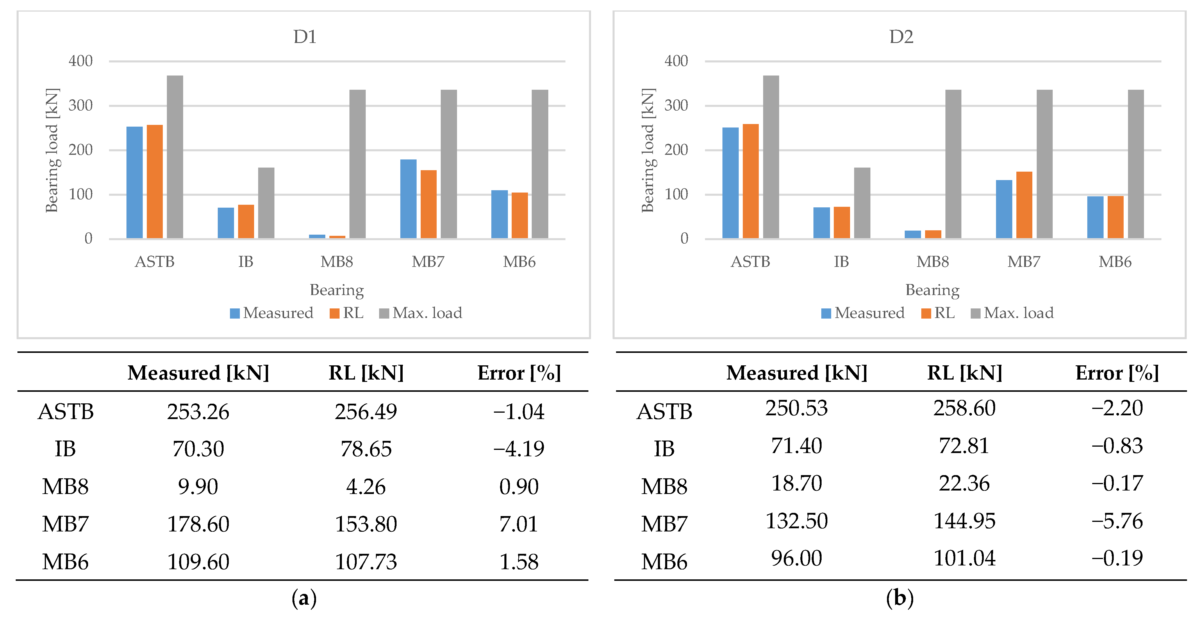
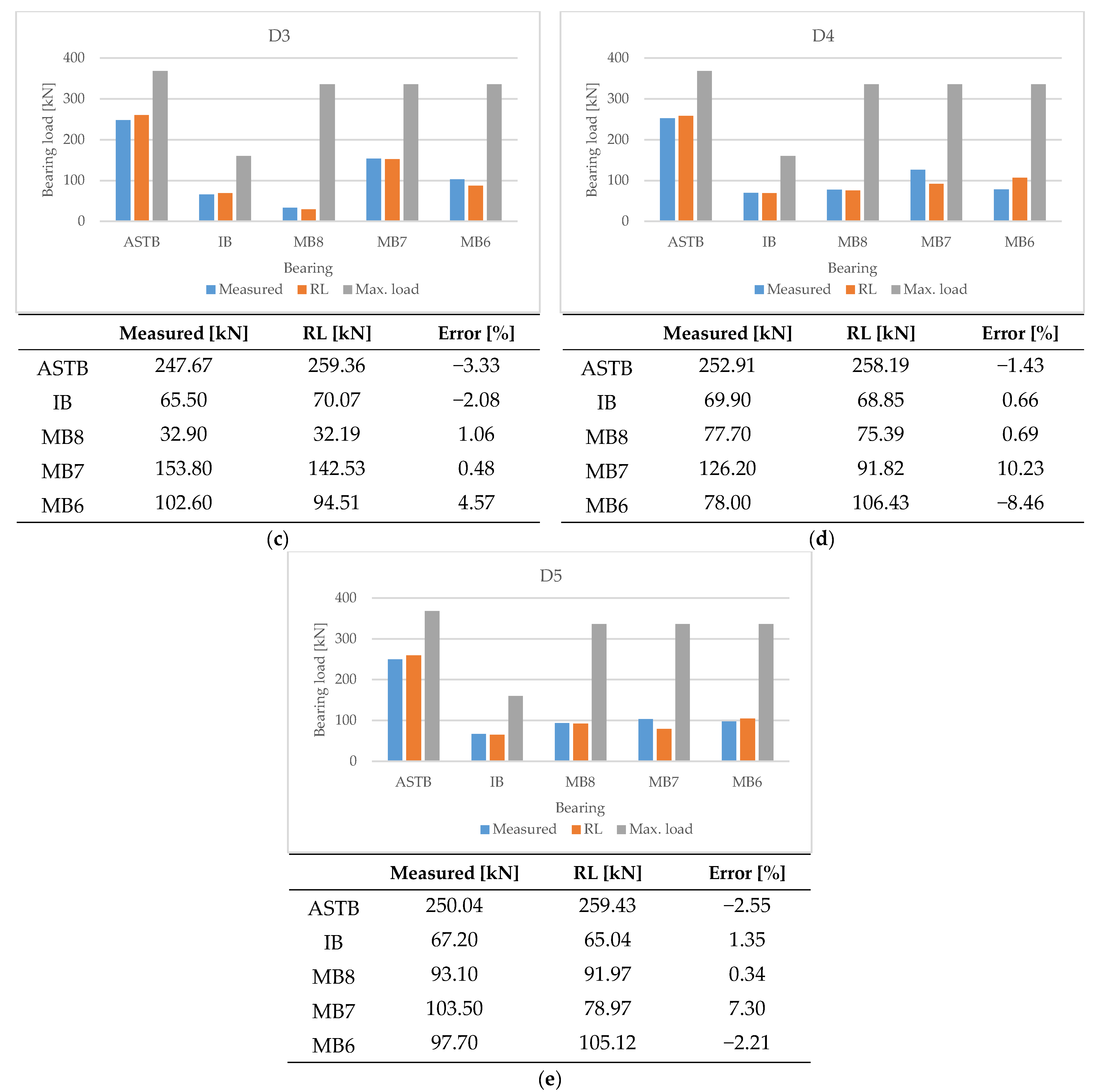
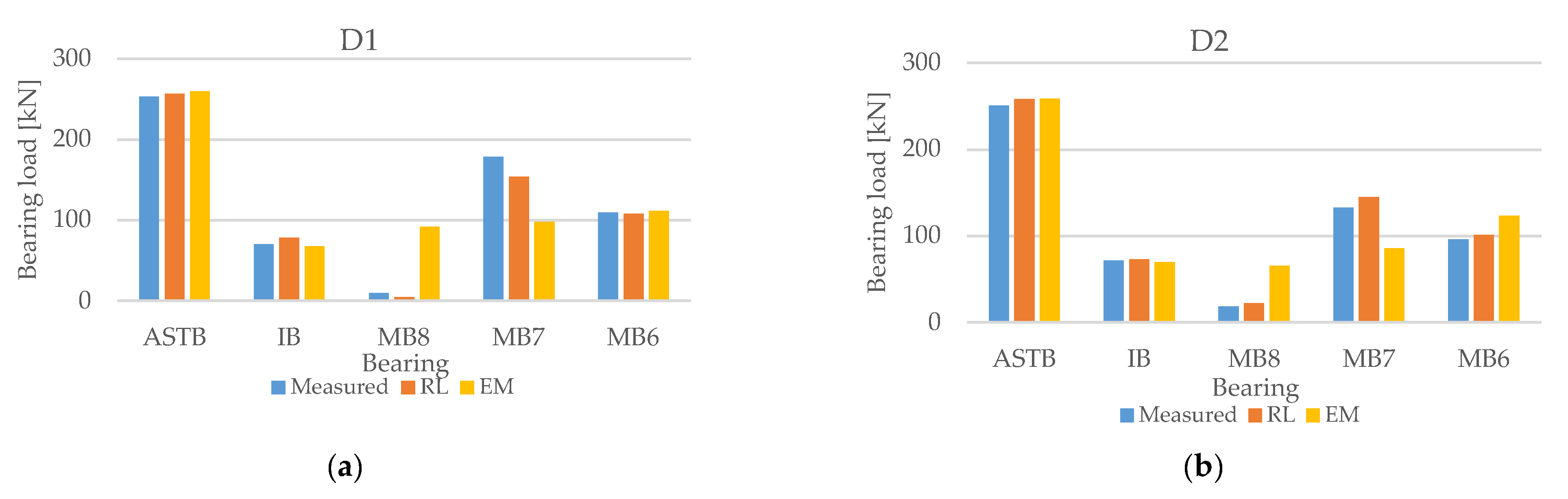
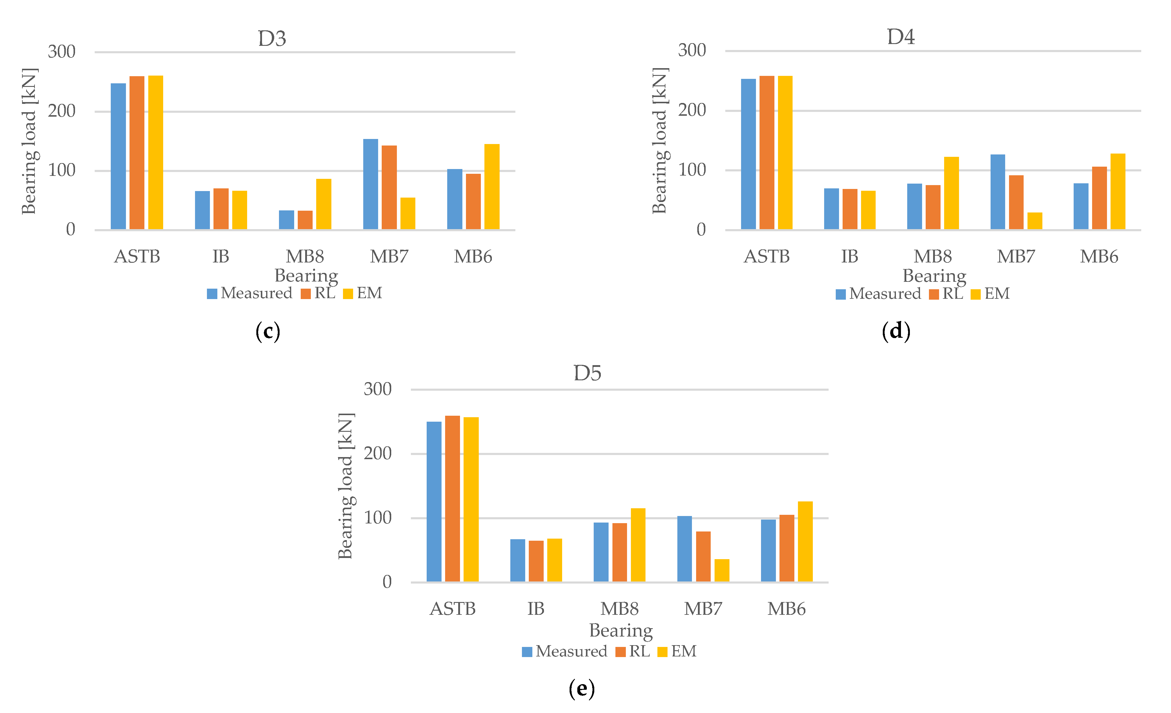
Figure 22.
Comparison of predicted bearing reaction force with measurements of (a) D1, (b) D2, (c) D3, (d) D4, and (e) D5.
Figure 22.
Comparison of predicted bearing reaction force with measurements of (a) D1, (b) D2, (c) D3, (d) D4, and (e) D5.
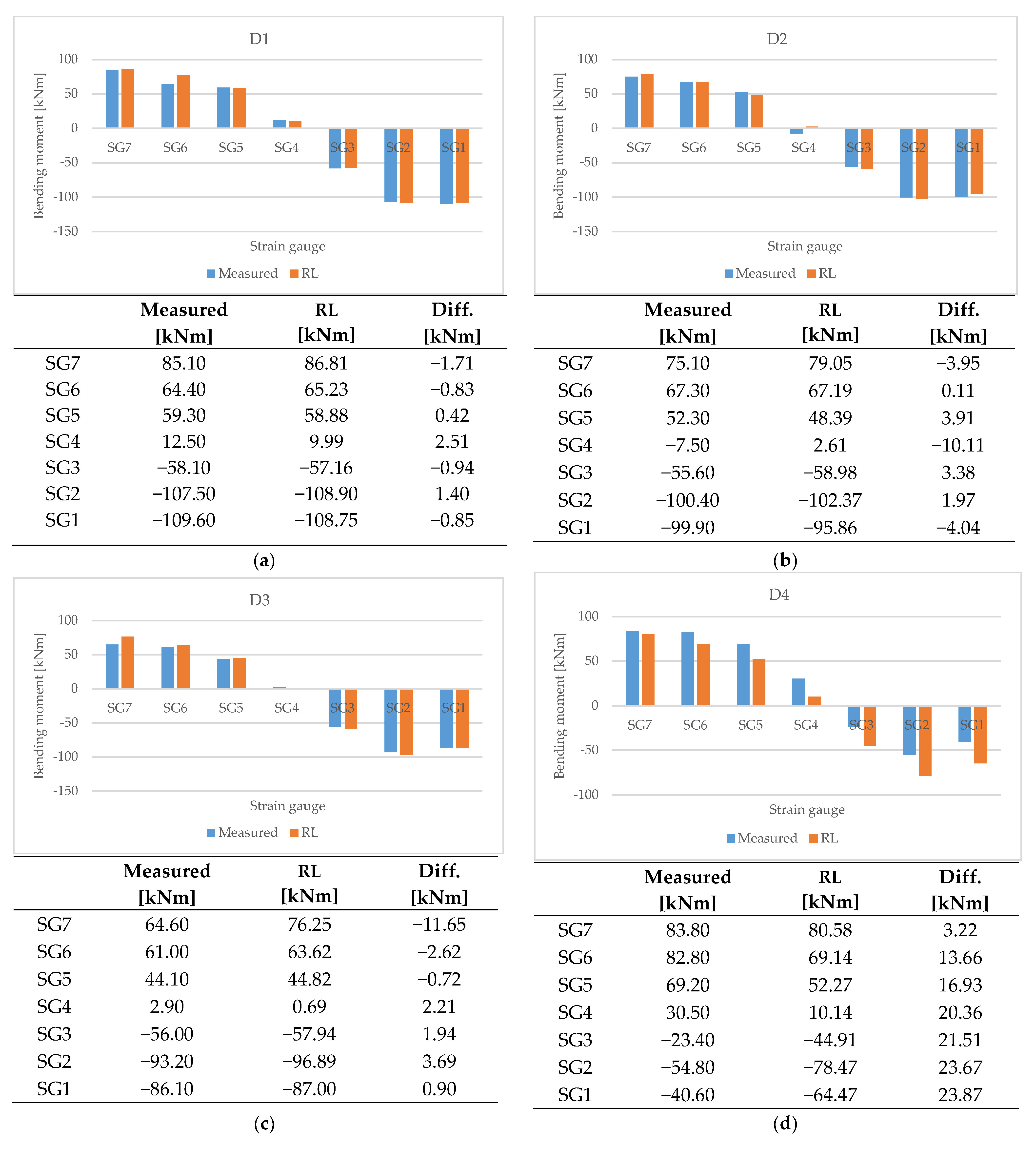
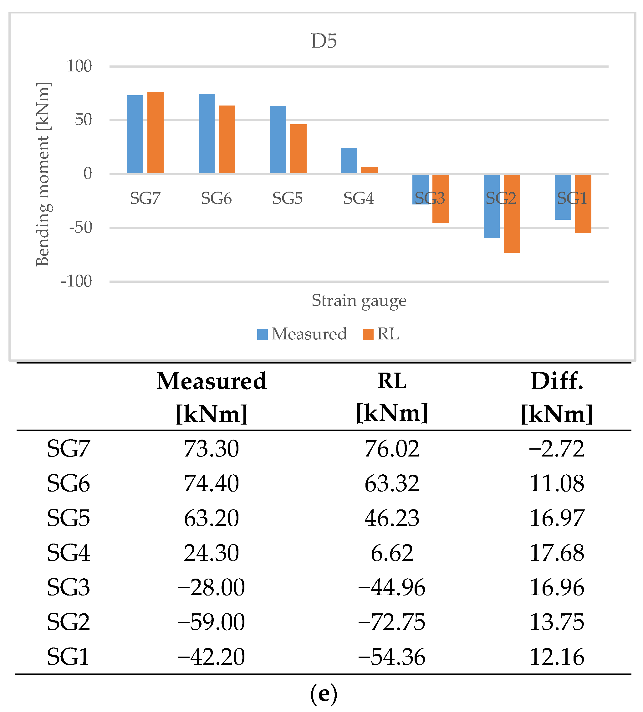
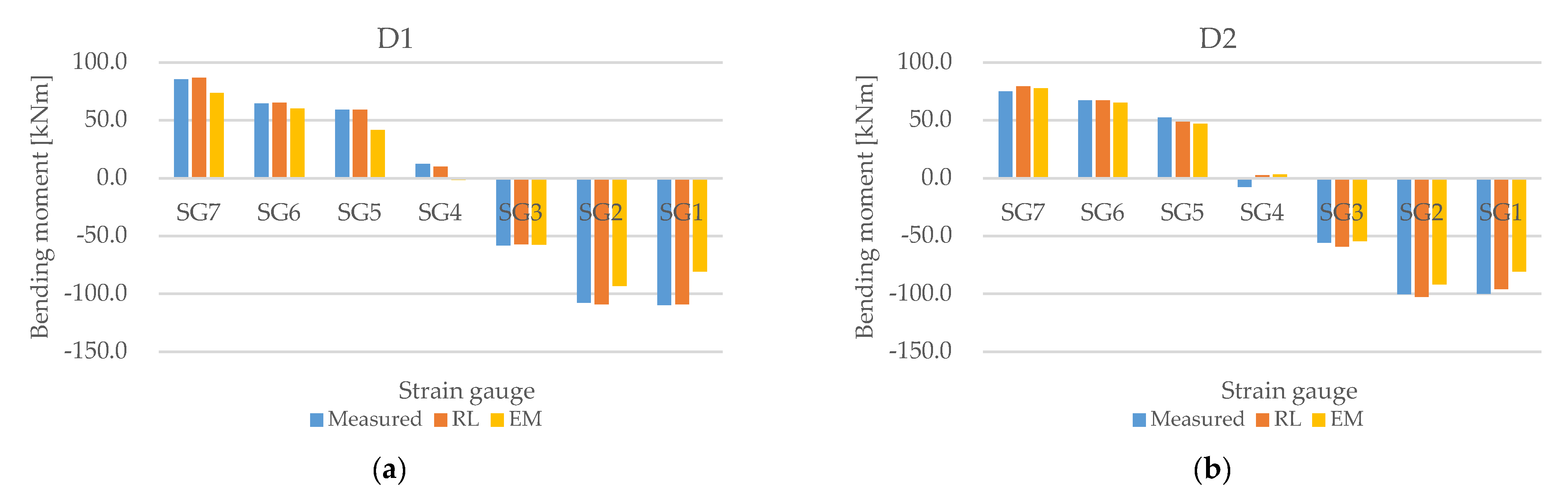
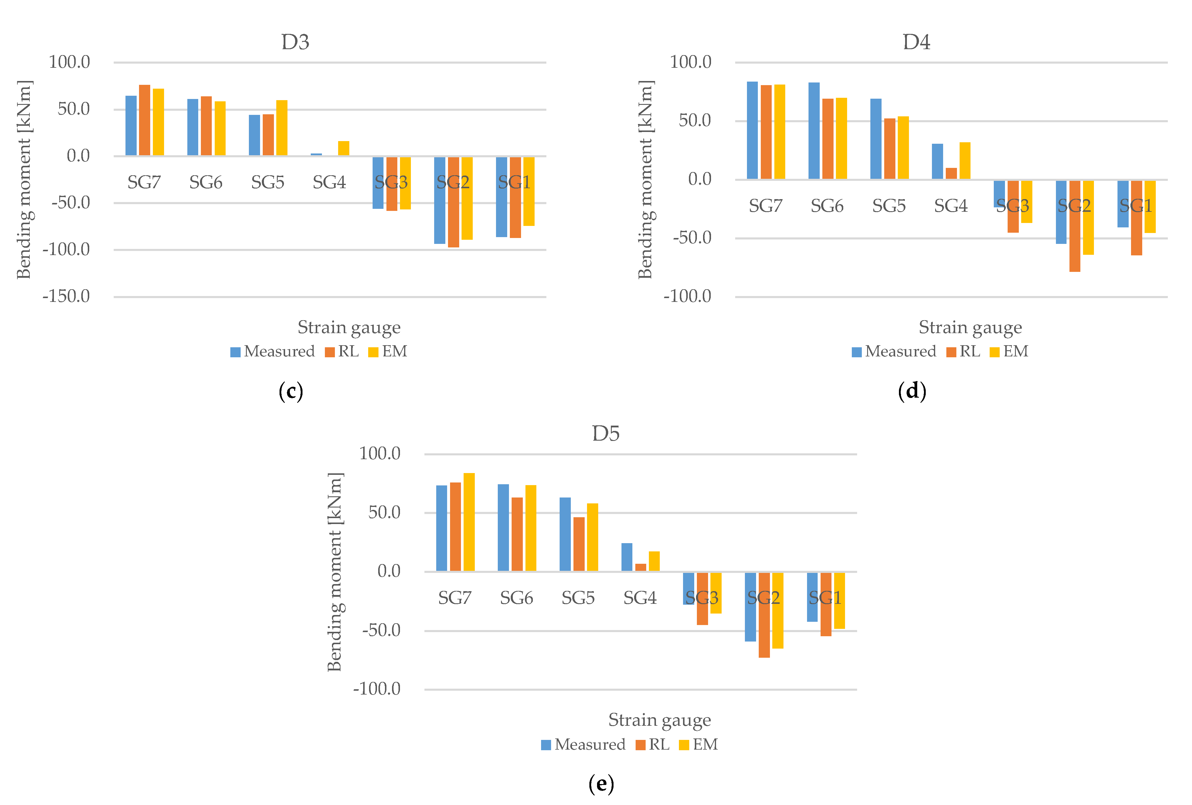
Figure 23.
Comparison of predicted strain gauge bending moment with measurements of (a) D1, (b) D2, (c) D3, (d) D4, and (e) D5.
Figure 23.
Comparison of predicted strain gauge bending moment with measurements of (a) D1, (b) D2, (c) D3, (d) D4, and (e) D5.
Figure 24.
Comparison of reaction force prediction of (a) D1, (b) D2, (c) D3, (d) D4, and (e) D5.
Figure 24.
Comparison of reaction force prediction of (a) D1, (b) D2, (c) D3, (d) D4, and (e) D5.
Figure 25.
Comparison of bending moment prediction of (a) D1, (b) D2, (c) D3, (d) D4, and (e) D5.
Figure 25.
Comparison of bending moment prediction of (a) D1, (b) D2, (c) D3, (d) D4, and (e) D5.
Table 1.
Specifications of target ship.
Table 1.
Specifications of target ship.
| Description | Value |
|---|
| GT [ton] | 29,327 |
| SDWT [ton] | 49,635 |
| Length OA [m] | 183.1 |
| Length BP [m] | 174.0 |
| Breadth MLD [m] | 32.2 |
| Depth MLD [m] | 19.1 |
| Draft design MLD [m] | 11.0 |
| Draft scantling MLD [m] | 13.2 |
| Year built | 2015 |
Table 2.
Specifications of shaft system of target ship.
Table 2.
Specifications of shaft system of target ship.
| Category | Description | Value |
|---|
| Main engine | Type | MAN B&W 6G50ME-B |
| MCR | 7700 kW × 93.4 rpm |
| NCR | 5344 kW × 82.7 rpm |
| Propeller | No. of blades | 4-blade fixed pitch |
| Diameter | 6600 mm |
| Material | Ni-Al-bronze |
| Mass in air | 18,200 kg |
| Cap & nut mass | 1538 kg |
| Flywheel | Mass | 11,207 kg |
Table 3.
Fore and aft drafts under measurement draft conditions.
Table 3.
Fore and aft drafts under measurement draft conditions.
| Draft Condition | Description | Fore Draft [m] | Aft Draft [m] |
|---|
| D1 | Light ballast APT empty | 3.40 | 6.60 |
| D2 | Ballast APT empty | 6.30 | 7.90 |
| D3 | Ballast APT full | 6.45 | 8.95 |
| D4 | Scantling APT empty | 13.50 | 12.50 |
| D5 | Scantling APT full | 13.20 | 12.60 |
Table 4.
Jack-up measurement results.
Table 4.
Jack-up measurement results.
| | D1 [kN] | D2 [kN] | D3 [kN] | D4 [kN] | D5 [kN] |
|---|
| IB | 70.3 | 71.4 | 65.5 | 69.9 | 67.2 |
| MB8 | 9.9 | 18.7 | 32.9 | 77.7 | 93.1 |
| MB7 | 178.6 | 132.5 | 153.8 | 126.2 | 103.5 |
| MB6 | 109.6 | 96.0 | 102.6 | 78.0 | 97.7 |
Table 5.
Detailed strain gauge attachment locations.
Table 5.
Detailed strain gauge attachment locations.
| Strain Gauges | Distance from Shaft End [mm] |
|---|
| SG7 | 5862 |
| SG6 | 6875 |
| SG5 | 8137 |
| SG4 | 8972 |
| SG3 | 10,467 |
| SG2 | 12,712 |
| SG1 | 14,422 |
Table 6.
Strain gauge measurement results.
Table 6.
Strain gauge measurement results.
| | D1 [kNm] | D2 [kNm] | D3 [kNm] | D4 [kNm] | D5 [kNm] |
|---|
| SG7 | 85.1 | 75.1 | 64.6 | 83.8 | 73.3 |
| SG6 | 77.4 | 67.3 | 61.0 | 82.8 | 74.4 |
| SG5 | 59.3 | 52.3 | 44.1 | 69.2 | 63.2 |
| SG4 | 12.5 | −7.5 | 2.9 | 30.5 | 24.3 |
| SG3 | −58.1 | −55.6 | −56.0 | −23.4 | −28.0 |
| SG2 | −107.5 | −100.4 | −93.2 | −54.8 | −59.0 |
| SG1 | −109.6 | −99.9 | −86.1 | −40.6 | −42.2 |
Table 7.
Calculation results of ASTB reaction force.
Table 7.
Calculation results of ASTB reaction force.
| | D1 [kN] | D2 [kN] | D3 [kN] | D4 [kN] | D5 [kN] |
|---|
ASTB
(calculated) | 253.26 | 250.53 | 247.67 | 252.91 | 250.04 |
Table 8.
Shaft FE model details.
Table 8.
Shaft FE model details.
| Description | Value |
|---|
| No. of nodes | 54 |
| No. of elements | 53 |
| Type of element | 1D beam element |
| Young’s modulus [N/mm2] | |
| Poisson’s ratio | 0.3 |
Table 9.
Shaft FE model applied loads.
Table 9.
Shaft FE model applied loads.
| | Position [mm] | Load [kN] |
|---|
| Bonnet | 290 | 8.813 |
| Propeller | 921 | 150.122 |
| Flywheel | 14,667 | 109.940 |
| Chain force | 15,375 | −99.900 |
| Crank | 16,242 | 125.000 |
| Crank | 17,136 | 125.000 |
| Crank | 18,030 | 125.000 |
| Crank | 18,924 | 125.000 |
Table 10.
Shaft FE model boundary conditions.
Table 10.
Shaft FE model boundary conditions.
| | Translations | Rotations |
|---|
| ASTB | Y, Z | - |
| IB | Y, Z | - |
| MB8 | Y, Z | - |
| MB7 | Y, Z | - |
| MB6 | Y, Z | - |
| MB5 | Y, Z | - |
| MB4 | Y, Z | - |
| MB3 | Y, Z | - |
| Shaft end | X, Y | X, Z |
Table 11.
Fluid density in contact with shaft FE model.
Table 11.
Fluid density in contact with shaft FE model.
| | Density [kg/mm3] | Start [mm] | End [mm] | Comments |
|---|
| Water density | | 0 | 1782 | Bonnet, propeller |
| Oil density | | 1782 | 4902 | ASTB |
| Shaft (in air) | | 4902 | 19,818 | IB, MB, flywheel, crank |
Table 12.
Deep RL applied hyperparameters.
Table 12.
Deep RL applied hyperparameters.
| Category | Description | Value |
|---|
| Q-value | Learning rate () | 0.001 |
| Discount factor () | 0.95 |
| -greedy policy | | 0.05~0.01 |
| Experience replay memory | Memory size | 200 |
| Batch size | 10 |
| Deep neural network | Hidden layer | 3 |
| Hidden layer node | 128 |
| Activation function | ReLU |
| Epoch | 1000 |
| Loss | Mean squared error (MSE) |
| Optimizer | Adam |
Table 13.
Allowable reaction force for bearings according to classification rules (ASTB, IB).
Table 13.
Allowable reaction force for bearings according to classification rules (ASTB, IB).
| | Max. Permissible Pressure
[MPa] | Bearing Area
(Diameter [
([ | Max. Ppermissible Load
[kN] | Min. Permissible Load
[kN] |
|---|
| ASTB | 0.8 | 0.46
() | 368.0 | - |
| IB | 1.2 | 0.1335
(30) | 160.2 | - |
Table 14.
Allowable bearing reaction force according to recommendations of main engine manufacturer (MBs).
Table 14.
Allowable bearing reaction force according to recommendations of main engine manufacturer (MBs).
| | Max. Permissible Load [kN] | Min. Permissible Load [kN] |
|---|
| MB8 | 336.0 | 0.0 |
| MB7 | 336.0 | 17.0 |
| MB6 | 336.0 | 17.0 |
| MB5 | 336.0 | 17.0 |
| MB4 | 336.0 | 17.0 |
| MB3 | 336.0 | 17.0 |
Table 15.
Shaft deformation prediction range.
Table 15.
Shaft deformation prediction range.
| | IB | MB8 | MB3 |
|---|
| | Min. [mm] | Max. [mm] | Min. [mm] | Max. [mm] | Min. [mm] | Max. [mm] |
|---|
| D1 | −1.7 | −1.0 | −5.5 | −4.0 | −4.8 | −3.0 |
| D2 | −1.7 | −0.6 | −5.3 | −2.9 | −4.5 | −1.8 |
| D3 | −0.8 | −0.2 | −3.2 | −1.5 | −2.9 | 0.2 |
| D4 | 0.3 | 0.5 | −2.3 | −1.4 | −1.9 | −0.5 |
| D5 | 0.4 | 0.5 | −1.6 | −1.1 | −0.9 | 0.0 |


