High-Resolution Observations of Upwelling and Front in Daya Bay, South China Sea

Abstract

Field observations of coastal regions are important for studying physical and biological features. Observations of high-resolution coastal phenomena were obtained by using a tow-yo instrument and a turbulence profiler at Daya Bay in the South China Sea in October 2015. Details of coastal phenomena, including warm water from a nuclear plant discharge, as well as an upwelling, and front, were obtained. The upwelling, with a width of 2 km, resulted in saltier and more turbid water near the bottom, with low chlorophyll-a and dissolved oxygen contents being transported upward to the surface layer and changing the local water environment. The front, with the lateral salinity variations as large as 0.7 psu across 1 km, was active at the water intersection of the South China Sea and Daya Bay. Such events commonly form during weak stratification periods in autumn. Continuous measurements from VMP-250 profiler over circa 22 h revealed active fronts and an averaged dissipation rate of 8 × 10⁻⁸ W/kg and diffusivity of 5.8 × 10⁻⁵ m²/s (i.e., one order of magnitude larger than in the open ocean) in the thermocline. The front was accompanied by strong mixing, indicating that it had formed at the intersection of different water masses and played an important role in energy dissipation in Daya Bay, further affecting the distribution of ecological elements.

1. Introduction

The South China Sea (SCS) is the largest marginal sea connected to the Western Pacific and is dominated by the East Asian monsoon. In winter, northeasterly winds overlie the SCS, whereas in summer, southwesterly winds prevail across the region [1,2]. In the Northern SCS, surface currents (e.g., the Kuroshio Current, South China Sea Warm Current, and cyclonic currents) display complicated dynamics. All of these large-scale currents are generally associated with wind, wind stress curl, and the processes from the Pacific [3,4,5,6,7].

Mesoscale to small-scale structures prevail in shelf seas of the Northern SCS, including eddies, fronts, and upwellings/downwellings [8]. These features play very important roles in regulating oceanic heat and energy exchange, are vital to the transport of biochemicals, and influence interannual/decadal climate variations [9]. Daya Bay (DYB) is located in the subtropical ocean and is one of the largest and most important gulfs along the southern coast of China. Physical and biochemical processes in DYB have been the focus of many previous studies. Thermal pollution has been identified in the vicinity of a nuclear power station in DYB [10]. High dissolved oxygen (DO) and nutrient concentrations were reported to be trapped within surface water [11,12]. The investigators surmised that the high surface nutrient concentrations resulted from stratification and the intrusion of upwelling water. The water refresh time was found to be approximately 26 days and wind driven. Fronts and associated eddies have been widely reported by oceanographers in Southern California [13], Africa [14], and Alaska [15]. Coastal fronts have mainly been examined at the interface of coastal water and the open ocean. According to their different formation mechanisms, coastal fronts can include tidal mixed, river plume, continental-shelf, upwelling, cape, and island fronts. Both eddies and fronts have mainly been observed via satellite or in situ ship-based observations.

Understanding the small-scale physical and biological processes in coastal and estuarine areas is a pressing issue in oceanography. In recent studies, small-scale physical processes in these areas have been observed [11,16,17]. Anthropogenic activities are considered the most important factor in the degradation of the DYB marine environment in recent years [10,18]. Therefore, studies of the hydrological and ecological processes in DYB are important for understanding the impacts of human activities on the ecology of DYB. Fixed-site and remotely sensed observations are commonly used in these studies [10,19,20,21,22]. For example, Tang et al. [10] obtained remote-sensing data from the Advanced Very High-Resolution Radiometer (AVHRR) satellite to study the thermal plume discharged by the nuclear power station into DYB and analyze its seasonal characteristics. Sun et al. [19] and Yang et al. [22] studied the long-term changes in phytoplankton response patterns in DYB, using fixed-site observations. However, satellite remote-sensing and fixed-site station observations have a disadvantage in that these observational methods cannot be used to obtain high-resolution internal profile characteristics. Satellite remote-sensing observation can only observe sea surface information. In situ conductivity–temperature–depth profiler (CTD) observation of fixed-site station often lacks continuity of spatial and temporal results.

Daya Bay covers an area of 600 km², with a width of approximately 15 km and a north to south length of approximately 30 km. It has a complex topography, contains many islands, and therefore, has a rich dynamic structure. Low-resolution station observations cannot be used to explain the structure of the fine-scale, dynamic thermal, and ecological processes in the bay. A useful method for observing oceanic processes is towed observation. With this method, high-resolution data can be obtained rapidly and continuously. In this study, we investigated the rich structural characteristics of DYB, which included the thermal plume discharged from the nuclear power station, as well as an upwelling, and front, using high-resolution Yoing Ocean Data Acquisition (YODA) profiler data and a microstructure turbulence profiler. We then describe the fine-scale and turbulence features of these structures.

2. Materials and Methods

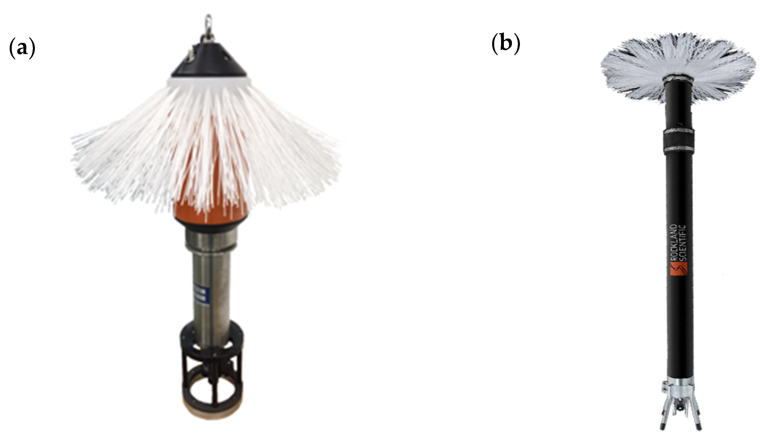
2.1. Instruments

The main data used in the study were collected by a YODA profiler and a VMP-250 turbulence profiler.

The YODA profiler (manufactured by JFE Advantech Co. Ltd., Japan; Figure 1a) is a tow-yo instrument that can be used to profile the water column with high resolution from small boats, without occupying much space [11]. The instrument is equipped with a deployment winch and sensors that measure conductivity, temperature, pressure, chlorophyll, turbidity, and DO. The brush at the top of the instrument provides a stabilizing effect on the free-fall sinking speed, which is approximately constant at 0.2 m/s. The sampling frequency is 10 Hz. All data are stored internally and downloaded to a PC through a wet connector and interface.

The VMP-250 (manufactured by Rockland Scientific inc., Canada; Figure 1b) is a coastal-zone profiler for the measurement of microscale turbulence. The profiler is designed for operation off small vessels with limited deck space (e.g., zodiacs) or where electrical power facilities are limited or missing (e.g., ice camps). The instrument is equipped with two shear probes, one thermistor, and a nose-mounted conductivity–temperature sensor. The VMP-250 has a constant free-fall sinking speed of approximately 0.7 m/s. The sampling frequency is 1024 Hz. All data are stored internally and downloaded to a PC through a wet connector and interface.

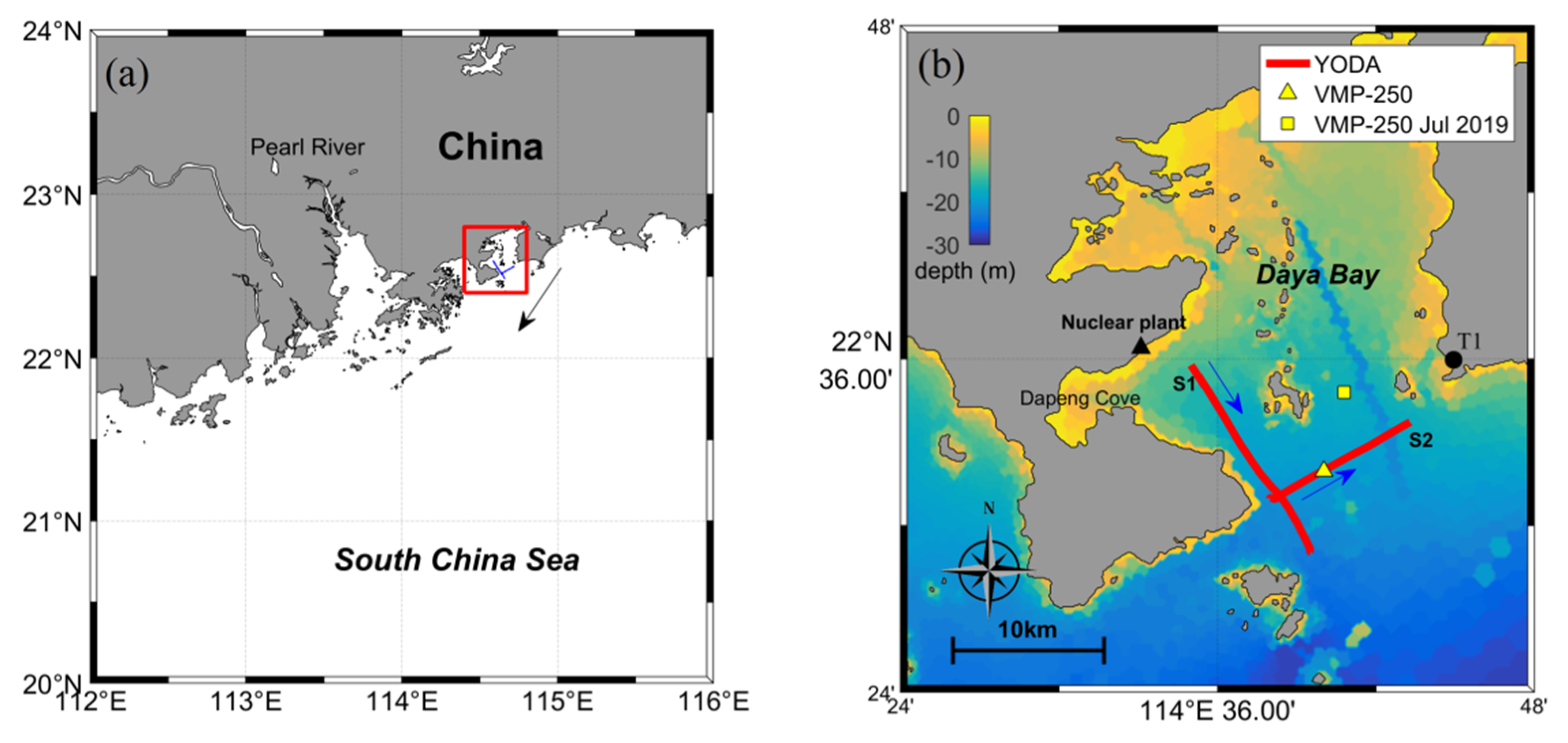
2.2. Observations

DYB is a large semi-enclosed bay (ca. 24 km in length and 13–25 km in width, covering an area of ca. 600 km²). The bay has an irregular coastline and contains more than 50 islands. It is located along the south coast of China (114°29.7′–114°49.7′ E, 22°31.2′–22°50.0′ N), as shown in Figure 2. Measurements were taken between 20 October and 22 October 2015. On 20 October 20 2015, we obtained conductivity, temperature, pressure, chlorophyll, turbidity, and DO data, using YODA along the western boundary of DYB (S1) and a cross-section of the mouth of the bay (S2) (Figure 2). The S1 observation transect ran from the north to the south, with the survey starting at 12:20 local time and ending at 14:50, whereas S2 ran from the west to the east, with the survey starting at 16:00 and ending at 18:30. During the cruise, YODA obtained 53 and 56 profiles at S1 and S2, respectively. The average space interval between successive YODA measurements was approximately 230 m, enabling fine-scale observations of physical phenomena.

The VMP-250 profiler was used to measure turbulence at a fixed station at the mouth of DYB (yellow triangle in Figure 2b). We obtained 74 turbulence profiles from 10:00 on 21 October to 7:30 on 22 October 2015. The time intervals between VMP-250 measurements ranged from 10 to 30 min; therefore, any rapid changes in physical phenomena could be observed.

There are no major rivers discharged into DYB, but three small streams discharged into Dapeng Cove. From September to October 2015, the average rainfall in DYB is less than 30 mm. The sea surface wind was northeasterly and was less than 10 m/s during the observation period, indicating that our observation was less affected by surface runoff and sea surface wind field. Therefore, the effects of rainfall, runoff and sea surface wind are ignored in the latter analysis. The tidal current in DYB is characterized by diurnal tide and semidiurnal tide and the semidiurnal tide is more prominent ([18]).

2.3. Calculation of Turbulence

The shear probes in the VMP-250 profiler measured high-frequency velocity fluctuations, which were used to calculate the local turbulent dissipation rate. The dissipation rate was estimated by using the following isotropic formula:

$$\epsilon =\frac{15}{2}v\overline{\left(\frac{\partial u}{\partial z}\right)}=\frac{15}{2}v{\displaystyle {\int }_0^{k_{max}}\psi \left(k\right)}\mathrm{d}k$$

(1)

where $\nu$ is the kinematic molecular viscosity, the overline indicates a spatial average, u is either one of the two horizontal components of velocity, z is the vertical coordinate, $\psi \left(k\right)$ is the spectrum of vertical shear, and k is the vertical wavenumber [23]. The upper limit of the integration, k_max, is variable. The k_max value was calculated by using the method recommended by Shang et al. [24], which states that it should be the smallest of the following values: the lowest frequency that shows corruption of the shear signal by vibrations, a wavenumber of 150 cpm due to the spatial resolution of the shear probe, the cutoff frequency of the antialiasing filter, an estimate of the wavenumber that resolves 90% of the shear variance according to the Nasmyth spectrum, using the method of Lueck [25], or the location of the spectral minimum determined with a low-order fit to the spectrum in log–log space. Diapycnal diffusivity [23] was calculated based on the dissipation rate (ε) and stratification as follows:

$${\kappa }_{\rho }=\Gamma \frac{\epsilon }{N^2}$$

(2)

where Γ is the mixing efficiency, which was set to 0.2. The stratification was calculated as follows: $N^2=-\frac{g}{\rho }\frac{\partial \rho }{\partial z}$, where g is the acceleration due to gravity.

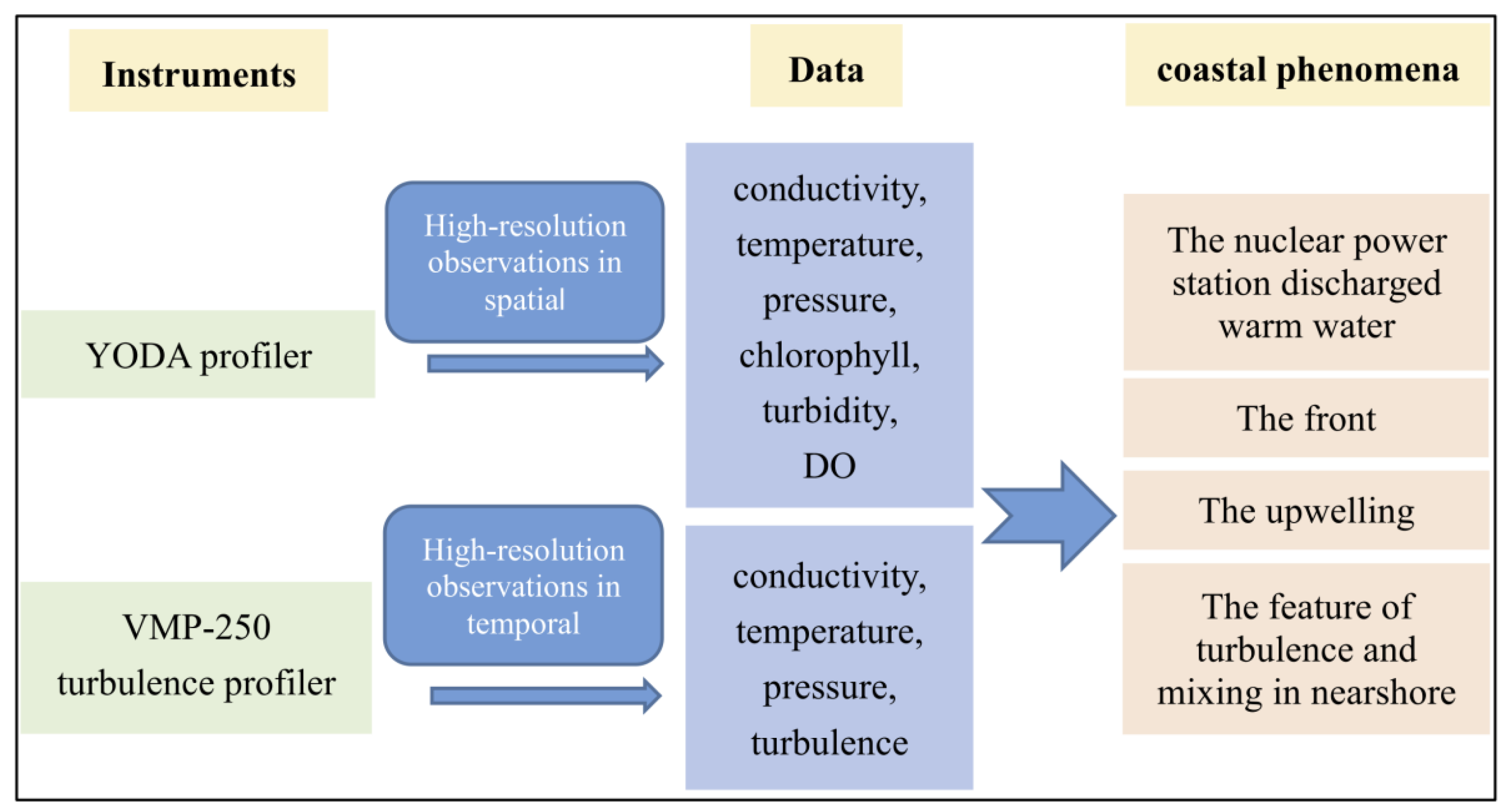
2.4. A Workflow Graph

Figure 3 provides a workflow graph to recap on the logic path of the study. The workflow mainly consists of three parts, including the used instruments, the data types, and the observed costal phenomena.

3. Results

3.1. High-Resolution Observations by YODA

In the section, features of coastal phenomenon, including the nuclear power station discharged warm water, upwelling and front, are revealed by high spatial resolution observations by YODA.

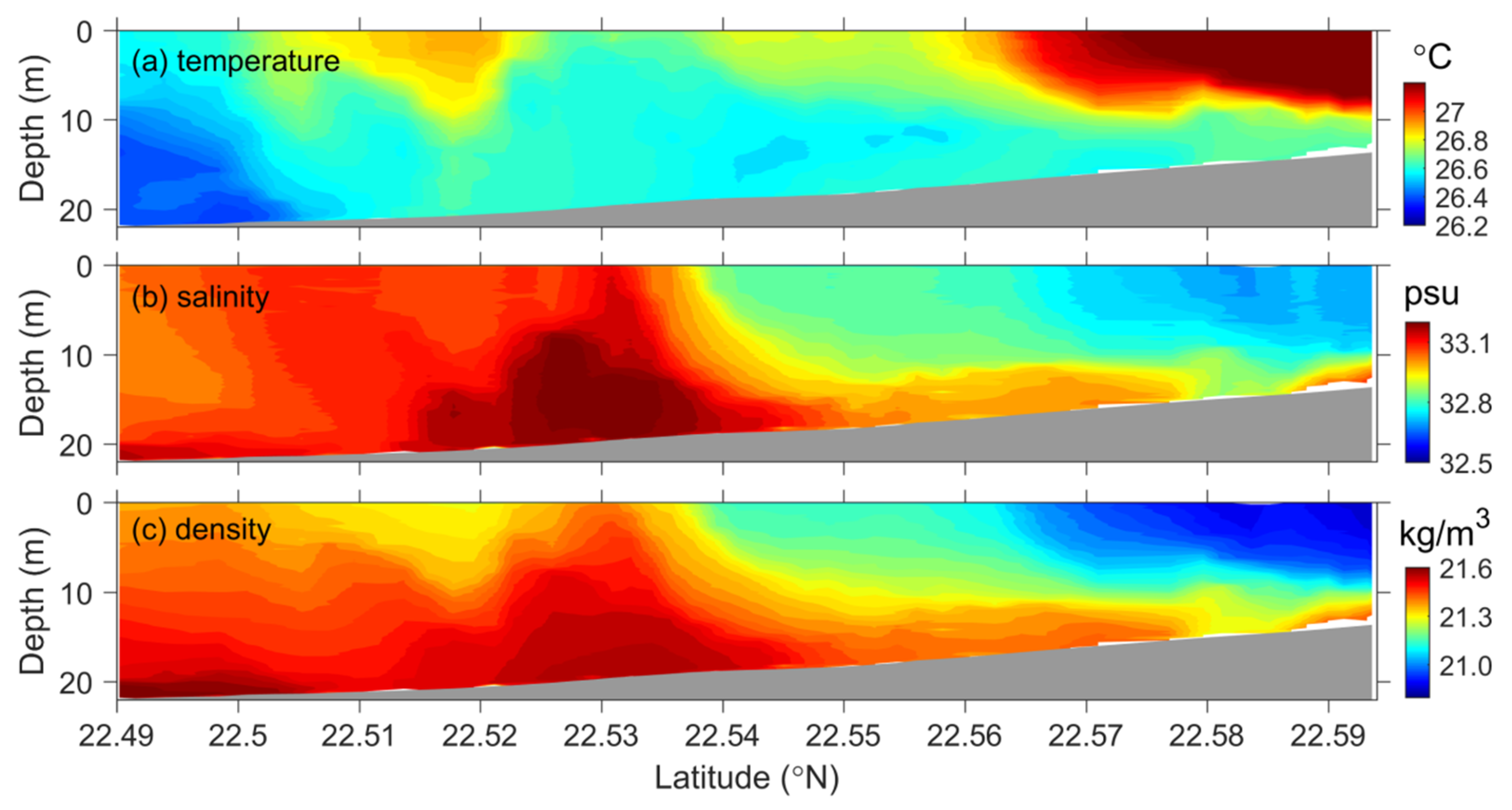
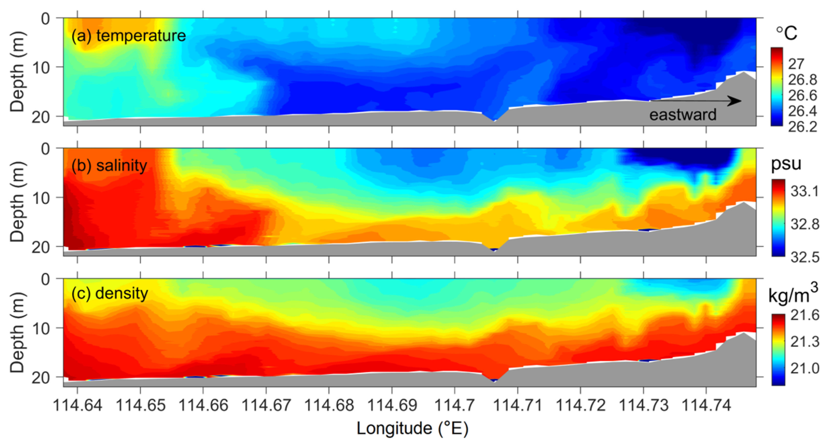
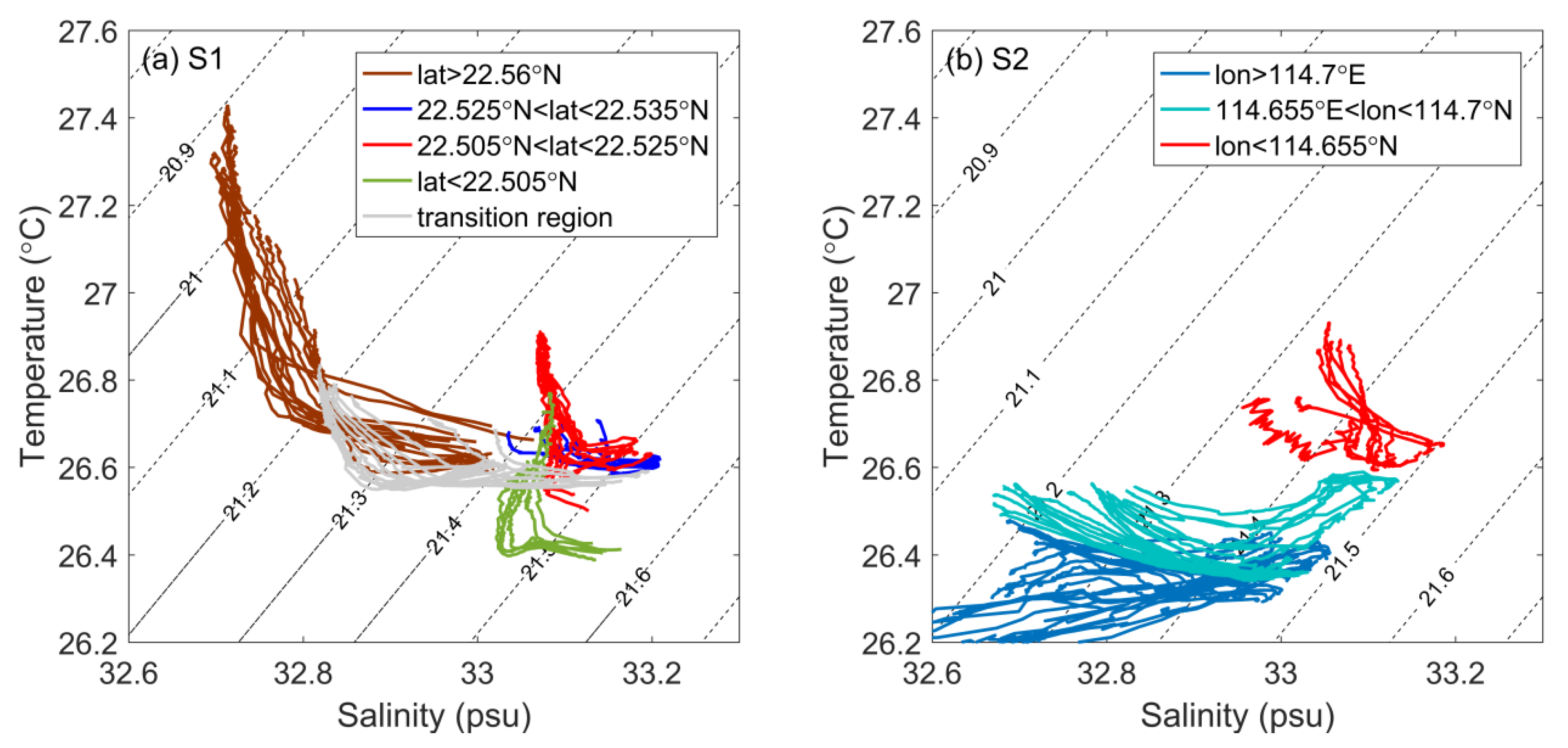
3.1.1. Water Properties

Our efforts to obtain high-resolution data for DYB by using the YODA profiler proved to be successful. Figure 4 and Figure 5 show the observed data, which indicated that the water environment of DYB was complex, with obvious horizontal spatial and vertical differences in temperature and salinity characteristics. The temperature varied from 26.2 to 27.4 °C, and salinity varied from 32.5 to 33.2 psu. The water along transect S1 was warm and fresh to the north, cold and salty in the middle, and warm and fresh farther to the south. The water was warm and salty to the west, and cold and fresh to the east. The temperature–salinity (T–S) sections (Figure 4 and Figure 5) and T–S diagrams (Figure 6) indicate that there were at least five distinct water masses along transect S1 and three distinct water masses along transect S2. The different water masses might have been formed by different dynamic characteristics.

The different water masses along transect S1 could be separated into the following five distinct areas. Area 1 had a latitude greater than 22.56° N, with warmer and fresher water found at the surface. Water in this area was affected by thermal discharges from the nuclear power station. Area 2 was found between the latitudes 22.525° N and 22.535° N, with saltier water present throughout the whole depth of the water column and no obvious changes in temperature with depth. Area 3 was found between the latitudes 22.505°N and 22.525° N, with warmer water present near the surface and no obvious changes in salinity with depth. Area 4 had a latitude lower than 22.505° N, with cooler water present throughout the whole depth of the water column. Area 5 was found between the latitudes 22.535° N and 22.56° N and represented a transition region.

The different water masses along transect S2 could be separated into the following three distinct areas. Area 1 had a longitude greater than 114.7° E, with cold and fresher water in the upper layer. Area 2 was found between the longitudes 114.655° E and 114.7° E, with saltier water present near the bottom and no obvious changes in temperature with depth. Area 3 had a longitude less than 114.655° E, with warmer and fresher water present near the surface. Generally, water on a shelf is cooler and fresher than in the adjoining ocean, leading to the formation of a shelf break front [26]. Therefore, it was reasonable to assume that the cold water at longitudes greater than 114.7° E originated from the bay. The area between 114.655° E and 114.7° E was considered a transition region.

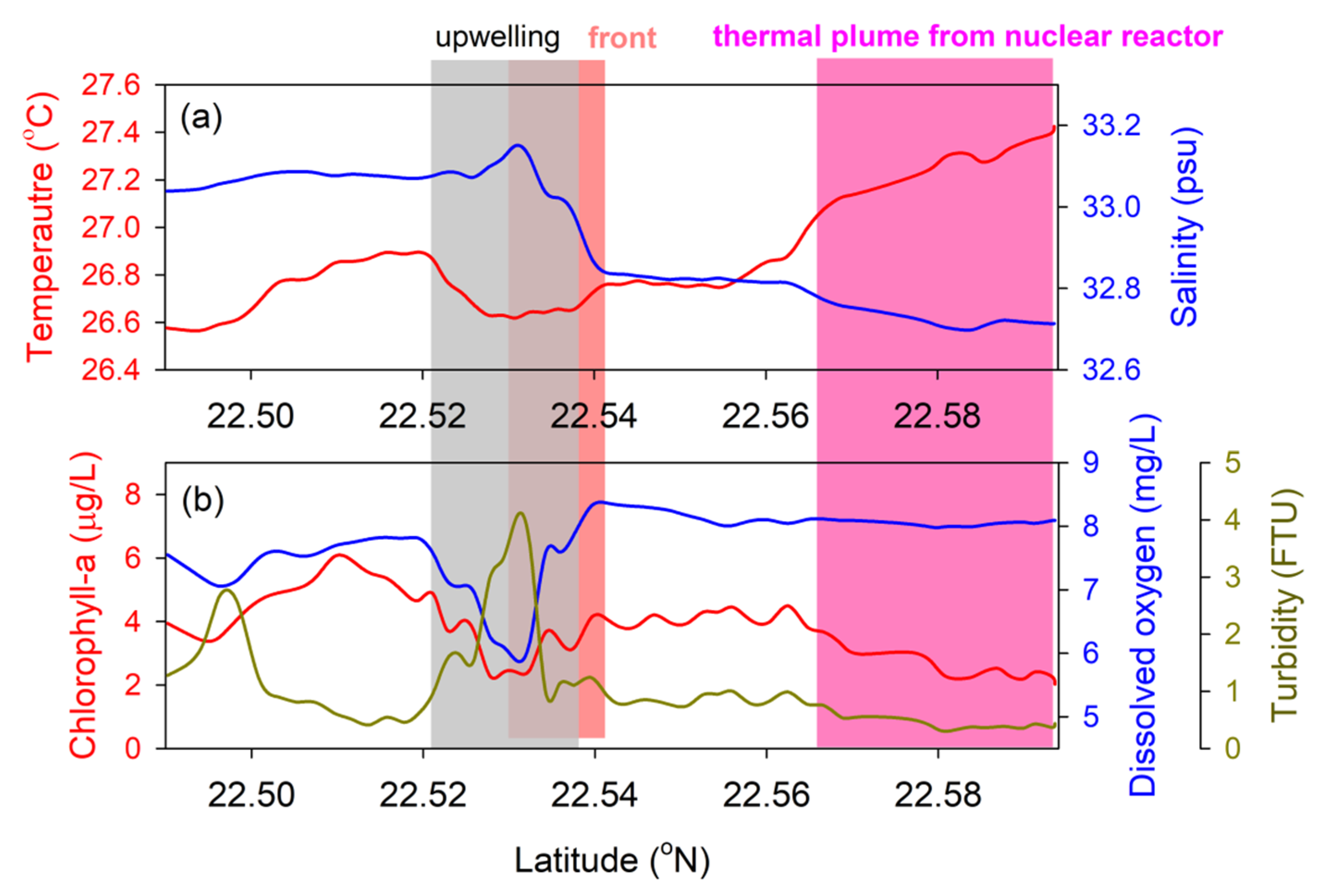
3.1.2. Influence of the Nuclear Power Station

Although the observation area was small, the water characteristics of DYB exhibited obvious spatial variability over a distance of approximately 12.5 km.

A significant feature of water temperature was that it was clearly affected by the thermal discharge from the nuclear power station in the north, and the temperature was significantly higher in the north than in other places (Figure 4a). The surface water temperature was as high as 27.4 °C in the northernmost observation position, which was approximately 2 km from the nuclear power station. This was 1 °C higher than the water temperature in the south. The warm water from the thermal discharge was mainly concentrated in the upper 10 m and extended approximately 5 km to the south of the release orifice, which corresponded to 22.56° N (Figure 4a). This range at which water discharge from the nuclear power station influenced water temperature was consistent with the satellite remote-sensing study of [10]. It has been reported that during the winter months, the thermal plume formed by water discharge from the nuclear power station is localized to an area within a few kilometers of the power plant. During the summer months, there is a larger thermal plume that extends 8–10 km south along the coast [10]. The strong seasonal difference in the thermal plume is related to vertical mixing in the water column in winter and stratification in summer. In addition to the warm water being discharged from the nuclear power station, a cloud of warm water with a radius of 2 km at the surface between 22.5° N and 22.52° N was also observed. This area of water was 0.3 °C warmer than the surrounding water. The temperature difference between the surface and bottom was less than 1 °C, indicating weak stratification of the water column during the observation period.

The salinity and chlorophyll-a content were also affected by the power plant. In the area influenced by discharge water, the salinity (Figure 4b) and chlorophyll-a content (Figure 7c) were lower than in the south. There was no significant difference in DO (Figure 7d).

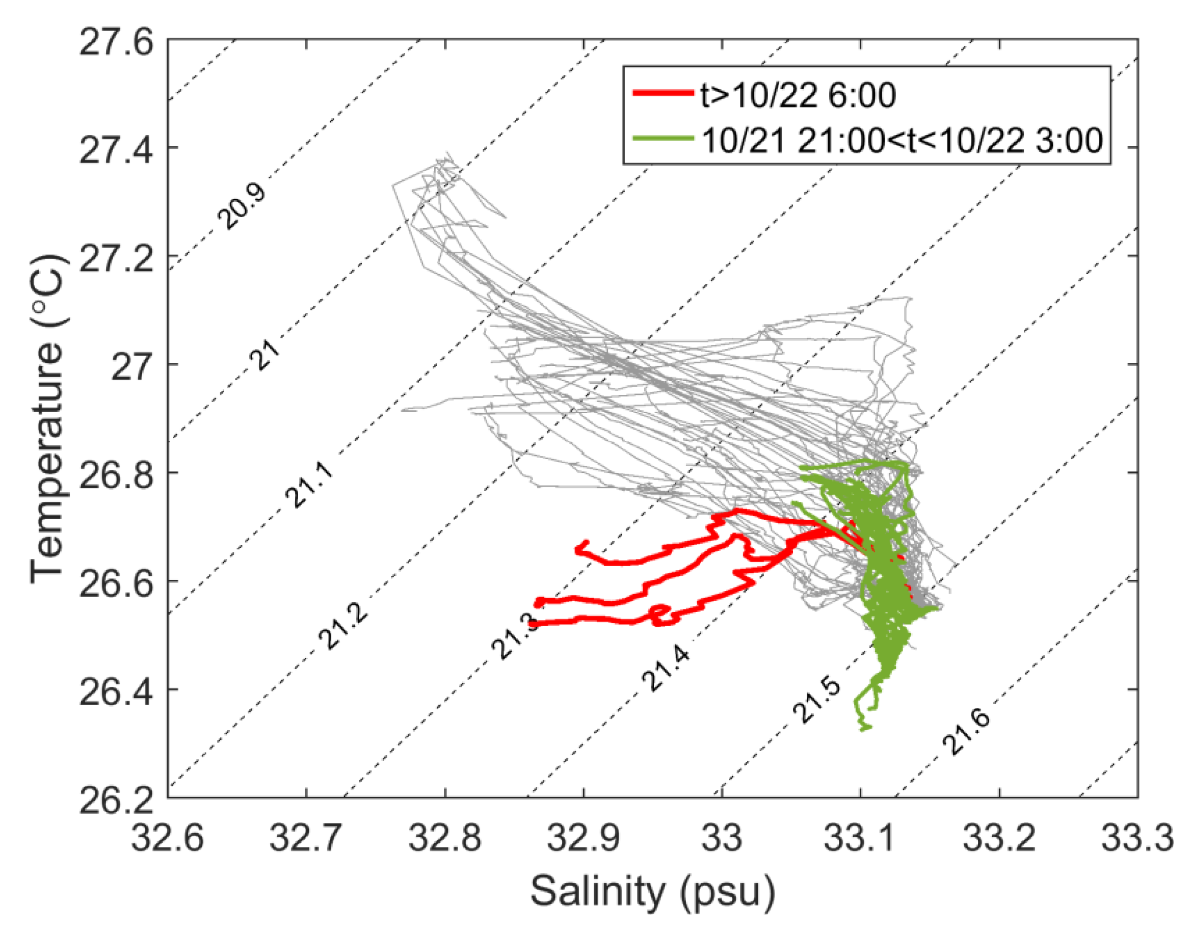
3.1.3. The Front

Water in DYB is cooler and fresher than in the adjoining SCS, resulting in a strong salinity front that is the most notable hydrographic feature in this region (Figure 4). There was a lateral density gradient identified along both transects S1 and S2. For transect S1, YODA measurements revealed lateral salinity variations as large as 0.7 psu across 1 km between 22.53° N and 22.54° N. Transect S2 also had a similar variation in salinity between 114.65° E and 114.66° E.

The width of the front was approximately 1 km, and the water depth, h, was 20 m. The Rossby deformation radius $R=\sqrt{g^{\prime }h}/f$ was approximately 6 km. The width of the front was much less than the Rossby deformation radius, indicating that it was not maintained by geostrophic balance. Here, g′ is the reduced gravity, which is given by $g^{\prime }=g\left(r_2-r_1\right)/r$, where r₁ and r₂ are the densities of the upper and lower layers, respectively, r is the mean density, g = 9.81 m/s², and f is the Coriolis parameter.

In the front area along transect S1, chlorophyll-a increased from 3 to 8 g/L, and the turbidity decreased from 4 to 1 FTU. We assumed that the strong front in S1 was formed at the intersection of different water masses and was strengthened by an upwelling system, in which cooler and saltier water at the bottom was dragged to the upper layer (Section 3.1.4). The presence of the front also prevented water from the adjoining SCS from entering the inner area of DYB.

3.1.4. The Upwelling

A cold salty water mass dominated the area between 22.52° N and 22.54° N. The turbidity was relatively high from the bottom to the sea surface, whereas the DO and chlorophyll-a concentrations were relatively low. The distributions of the parameters indicated a pumping process. The width of the upwelling was approximately 2 km. The most direct evidence of upwelling was the turbidity signal. Figure 7e shows that the turbidity was much higher at depth than in the upper layer. It was induced by friction between water layers, making the water in the bottom boundary layer turbid. In the area between 22.52° N and 22.54° N, the whole water column was more turbid than the surrounding water. This could only be explained by the turbidity of the entire water body being derived from the turbid water body at the bottom.

The occurrence of an upwelling is closely related to wind conditions. In the Northern Hemisphere, when the wind blows parallel to the coast for a long time, under the action of a geostrophic deflection force, the wind drift formed by the wind causes the surface water to leave the coast. This in turn causes the shallower water near the shore to rise and form an upwelling. In the North SCS, the most notable upwellings are the Eastern Guangdong upwelling and the Eastern Hainan upwelling, which occur in summer months [27,28,29]. In some case, the wind in particular direction acting on the vorticity field can generate vertical motions. For example, Chang et al. [30] reported that the seaward increasement of cyclonic vorticity near the Kuroshio’s western edge favors a stronger Ekman transport away from the jet, producing upwelling at the shelfbreak under a northeasterly wind. The passage of high-energy atmospheric systems also may stir up the upwelling [31]. In this study, however, the upwelling mechanism described above cannot explain the upwelling observed here in October. The upwelling areas caused by large-scale wind fields are more extensive than the upwelling area observed in this study, which had a width of approximately 2 km. The sea surface wind field far from the high-energy atmospheric system during the observation period is also not a cause of the vertical motions of water.

When the surface water is blocked by the coast or an island, sea water will gather and diverge in the horizontal direction, and an upwelling may occur in the vertical direction. In the study region, the terrain is flat in the area where the upwelling was observed (Figure 1), which indicates that the upwelling was induced by other dynamic mechanisms.

We assumed that the upwelling was formed by the interaction between tidal currents and the topography. Upwelling can bring nutrients from the bottom layer to the surface layer, make plankton grow in large quantities, and provide food for fish. Therefore, upwelling areas are often important fishing grounds, such as the Peru fishing grounds, which benefit from the cold Peru Current (upwelling compensation current). In our study area, the upwelling may also have an important impact on the local environment. As shown in Figure 7 and Figure 8, the upwelling changed the distribution of chlorophyll-a and DO in the local area and carried turbid material from the bottom up to the surface.

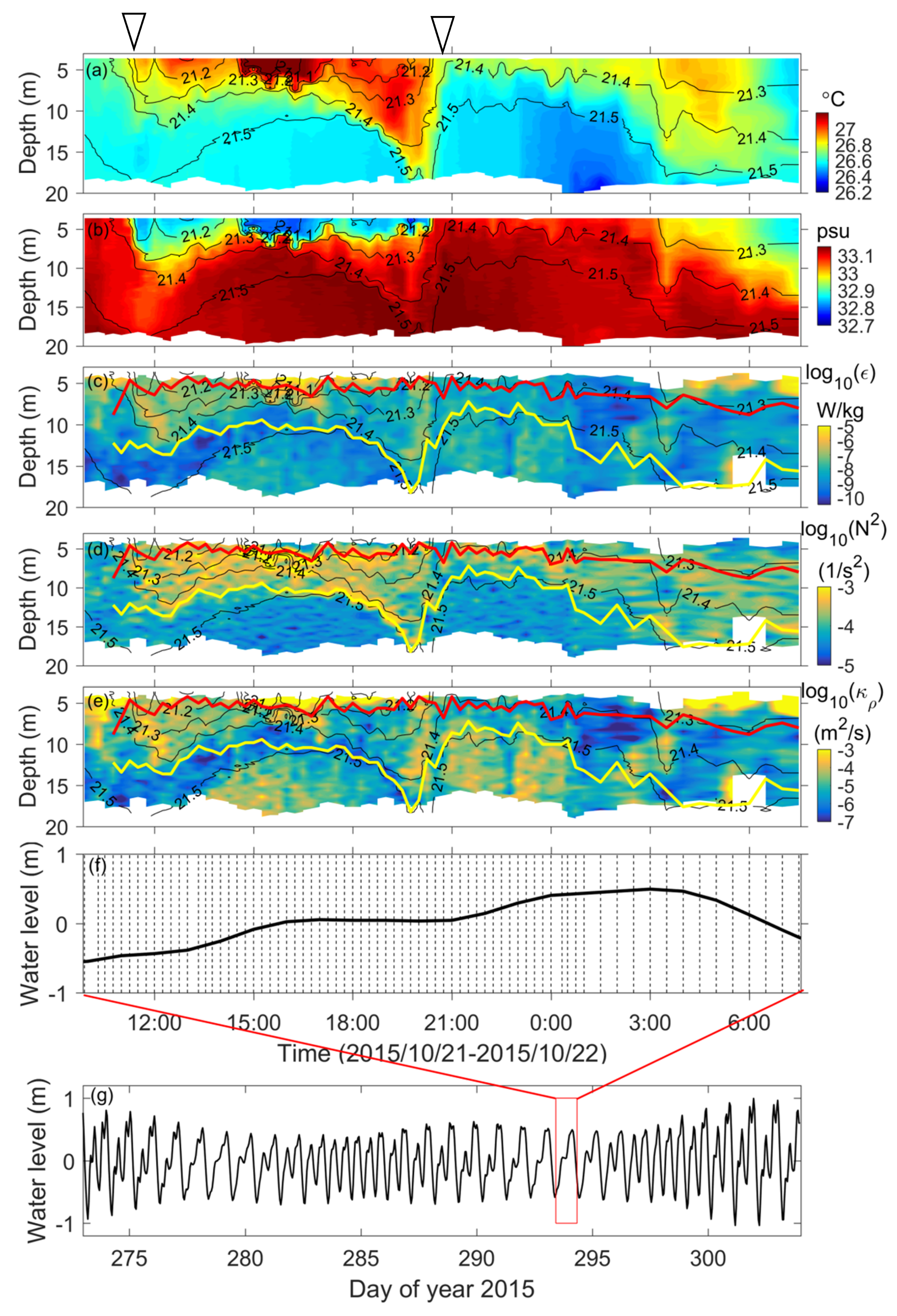
3.2. High-Resolution Observations by the VMP-250 Profiler

In the section, feature of coastal phenomenon of front and its accompanied turbulence are revealed by high temporal resolution observations by YODA.

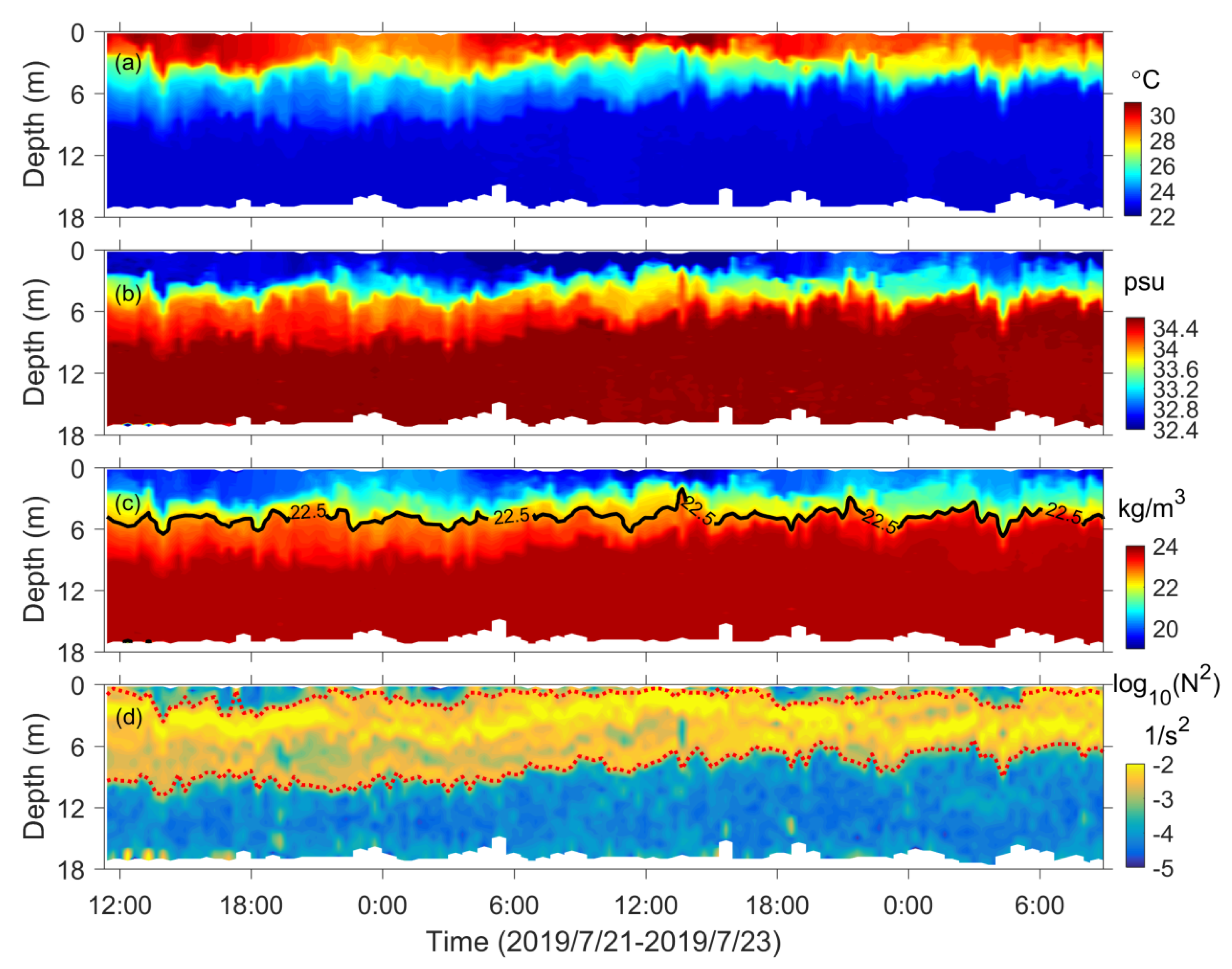
3.2.1. Water Properties

We used the VMP-250 profiler to observe turbulence for 22 h at a fixed location and obtained 74 profiles. The time intervals varied between 10 and 30 min (Figure 9c). A nose-mounted conductivity–temperature sensor was installed on the VMP-250 profiler, enabling the analysis of temperature and salinity characteristics observed at continuous monitoring stations.

The measurements indicated that both the temperature and salinity changed rapidly with time. Using density data, we calculated the depth of the surface mixed layer and the thickness of the bottom mixed layer (Figure 9c). The depth of the mixed layer was defined as the point at which the density varied by less than 0.05 kg/m³. The depth of the upper mixed layer was 8 m, whereas the thickness of the bottom mixed layer extended to 8 m (the water depth at the observation station was ca. 20 m). Sometimes, a bottom mixed layer could not be discerned. Activities in the upper water extended to the sea bottom at times (e.g., at 20:00 on 21 October 2015). The bottom mixed layer was mainly affected by tides, with the mixed layer depth increasing at high tide (Figure 9c,f). The largest buoyancy fluxes were in the stratified region just above the bottom mixed layer (Figure 9d).

The T–S sections and T–S diagrams (Figure 10) indicate that the water masses at various stations comprised distinct water masses. For example, between 21:00 on 21 October 2015 and 3:00 on 22 October 2015, the water temperature was low and salinity was high, especially in the bottom mixed layer. This was a period of high tide, indicating that SCS water was dominant during this period. From 6:00 to 8:00 on 22 October 2015, the upper layer of water exhibited a low temperature and low salinity. This was the ebb tide period, indicating that DYB water was the dominant water mass. Compared with the Figure 6, the characteristics of the seawater was confirmed. The observation station was located at the confluence of the SCS and DYB, which changed constantly under the action of tides. With the interactions at the confluence, an abundance of thermohaline structures was formed.

3.2.2. The Front

In addition to YODA measurements, lateral density gradients were also identified in the study area from the fixed station observations (Figure 9). These gradients were controlled by variations in both salinity and temperature. Stratification persisted throughout the upper water column, with considerable variability along isopycnal. VMP-250 measurements indicated lateral temperature variations as large as 0.4 °C and lateral salinity variations as large as 0.3 psu over 30-min periods at 11:30 and 20:30 on 21 October 2015. It is noted that the conventional definition of density front (dρ/dx) is related to the variation of horizontal distance of density. Here, we assume that the density front does not change in a certain period of time when it moves in the flow direction, dρ/dt = Udρ/dx. Thus, the larger the variation in dρ/dt, the stronger the density front. There were two strong fronts at these two moments, with density variations of approximately 0.2 kg/m³ over a 30-min period. At 20:30 on 21 October 2015, the front extended to the bottom. The width of the front was approximately 1 km (Section 3.1.3), and it took approximately 30 min for the front to cross the observation position. Therefore, we inferred that the speed of the front was approximately 0.5 m/s, which is similar to the tidal current velocity [18].

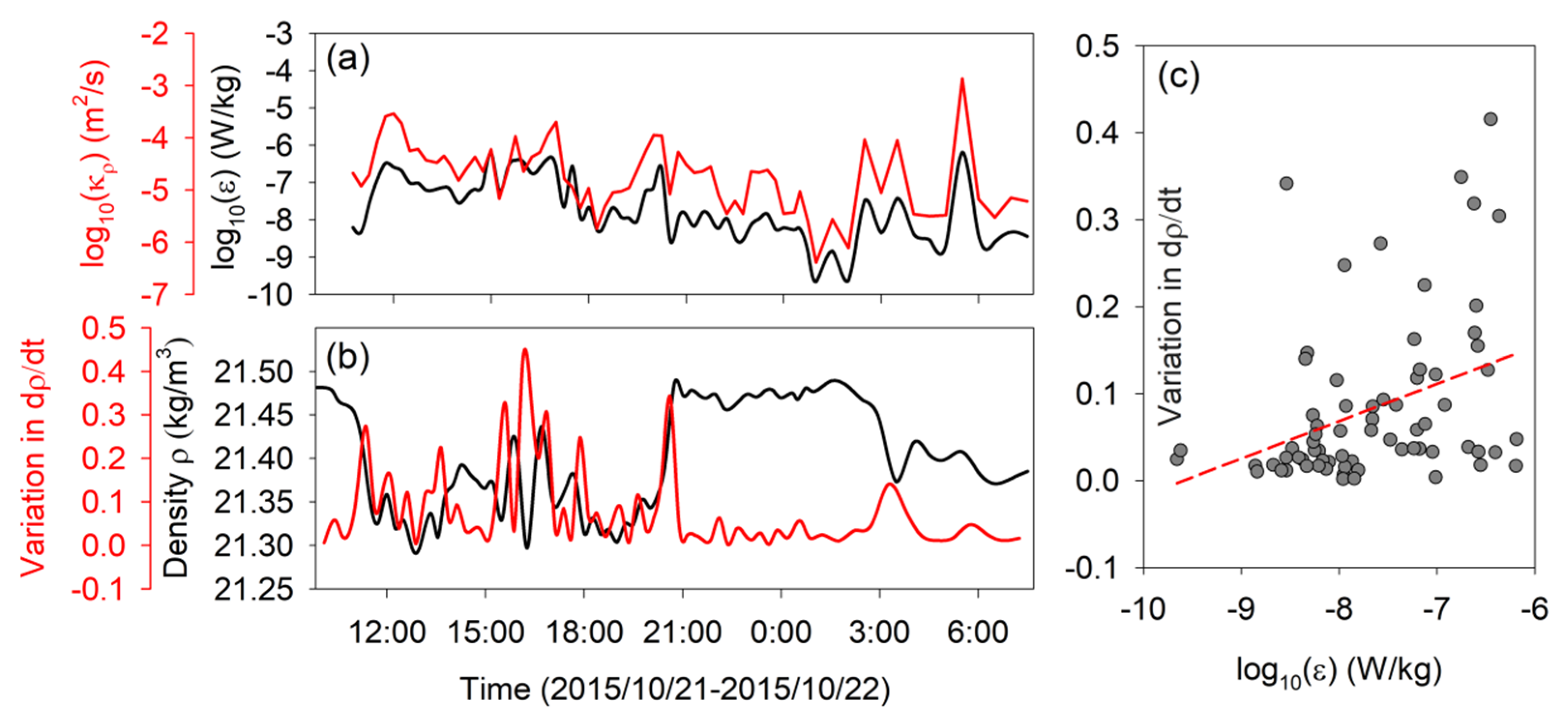
3.2.3. Turbulence

Examples of dissipation spectra at specified depth segments from the VMP-250 measurement at 12:15 on 21 October 2015 are shown in Figure 11. There were two shear probes installed at the head of profiler, and data from both probes are shown. The spectra were approximately consistent with the Nasmyth universal spectrum, indicating the credibility of the measurement. The triangles indicate the upper limit of integration. The raw microscale velocity shear was weak between 4 and 8 m; therefore, the estimated dissipation rate was small (ε~10⁻⁷ W/kg). The microscale velocity shear strengthened between 8 and 12 m, as did the dissipation (ε~10⁻⁶ W/kg).

It has been reported that dissipation and mixing on the shelf are mainly controlled by near-bottom friction and shear from low-frequency internal waves and solibores [26]. However, according to our observations, the front that formed at the intersection of the SCS and DYB also plays an important role in local energy dissipation. Figure 9c shows the dissipation rates and associated diapycnal diffusivities for each profile. The dissipation rates of the thermocline and bottom boundary layer were of the same order of magnitude. The thickness of the bottom mixing layer has the characteristics of periodic variation, and its increase is consistent with the period of high tide. The dissipation rate at the bottom also increase during the high tide periods (Figure 9e). Taken together with Figure 9c,e,f, it was concluded that the turbulence in the bottom mixed layer was driven by tidal currents. In the upper mixing layer, ocean mixing is mainly controlled by buoyancy flux and wind momentum flux [32]. In this study, we focused on the dissipation in the thermocline.

The dissipation rate of the thermocline was mainly between 1 × 10⁻⁹ and 1 × 10⁻⁶ W/kg, with an average value of 8 × 10⁻⁸ W/kg. The maximum value was mainly recorded at 11:30, 16:00, and 20:30 on 21 October 2015, as well as 3:00 on 22 October 2015, at which point the density profile changed substantially. Peak dissipation at 5:00 on 22 October 2015 was induced in a patch near the bottom. Average diffusivity profiles were calculated from the average dissipation rate and stratification. Because diffusivity was not well defined in the well-mixed boundary layers, average diffusivity profiles are only shown for data excluding the boundary layer (Figure 12a). The average diffusivity associated with mid-column, stratified turbulence was 5.8 × 10⁻⁵ m²/s for the whole profile, which is one order of magnitude greater than the level in an open-ocean thermocline [33,34].

To analyze the relationship between front and turbulent mixing in the thermocline, the density of water was averaged, excluding the boundary layer. Changes in average density with time (dρ/dt) were calculated. Active fronts existed on 21 November but there were fewer fronts on 22 November (Figure 12b). The fronts detected between 15:00 and 18:00 on 21 October 2015 were affected by the variation in density near the surface mixed layer. It can be seen from Figure 10 that the dissipation rate and variation in dρ/dt were positively correlated, i.e., a larger dρ/dt tended to produce a larger dissipation rate. This indicates that a density front in the study area is important for locating the sources of energy dissipation.

The turbulent mixing process in the ocean determines the redistribution of seawater characteristics. This plays a key role in the redistribution of nutrients, DO, and other ecological elements and substances in the ocean, which then affects marine productivity [35,36,37,38]. In this study, we did not make observations of ecological elements when VMP-250 measurements were recorded. However, it was apparent that the front regulated the distribution of ecological elements (Figure 7), while turbulent mixing also played an important role.

4. Discussion

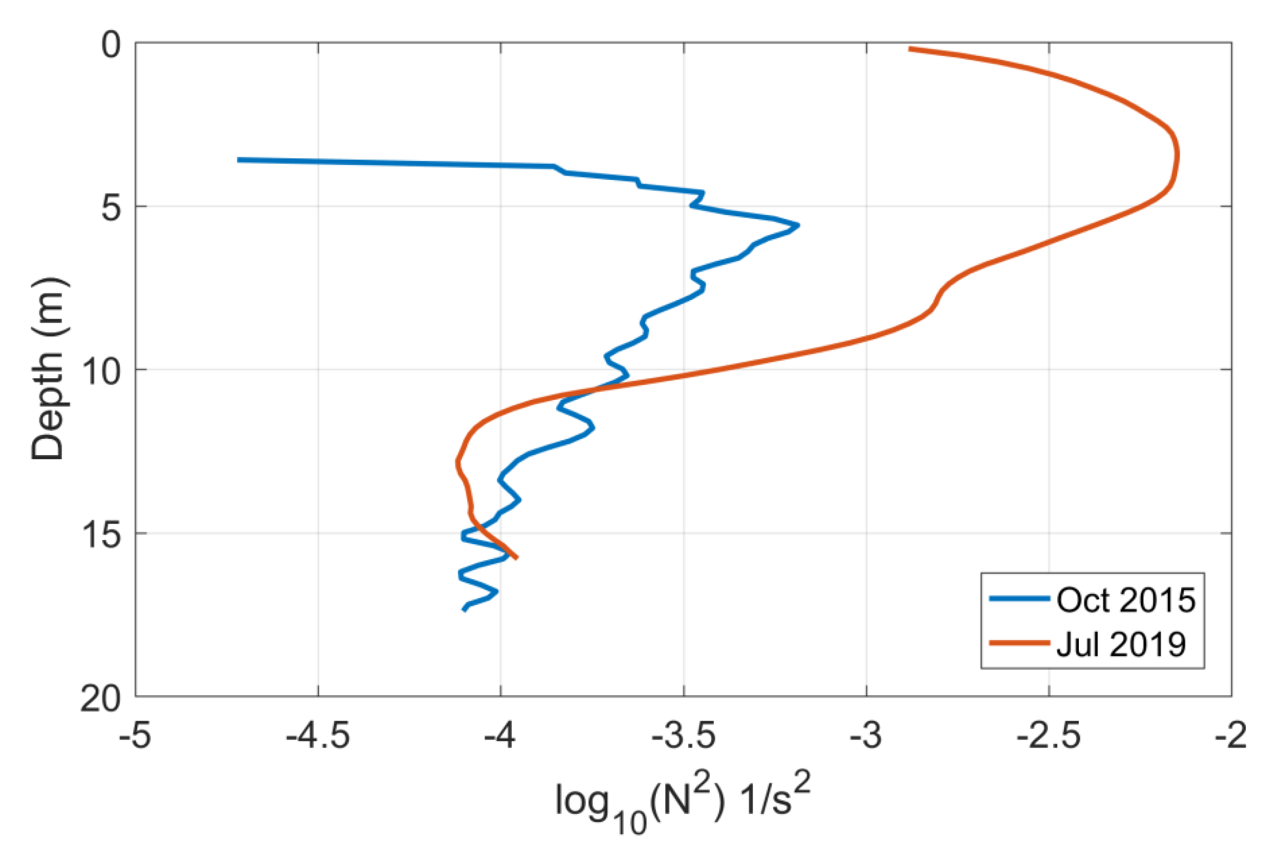
Comparison with Observations in July 2019

Daya Bay is located in the tropical monsoon region. In this area, the northeast monsoon is strong in winter, whereas the weaker southwest monsoon is dominant in summer [39]. During winter, the water in DYB is vertically mixed under the influence of the northeast monsoon [40]. Water stratification in DYB varies seasonally. The development of physical phenomena in the ocean is closely related to stratification, and seasonal variation in the formation of a front and its effect on energy dissipation in the observation area was obvious.

To confirm the seasonal variation in the front in DYB, we analyzed observations of the area (114.68° E, 22.58° N) from July 2019 (Figure 1). At the observation site, 138 profiles were obtained by YODA within 48 h, with a time interval of 20 min. The temperature difference between the surface and bottom was more than 6 °C, and the salinity difference was more than 2 psu (Figure 13), which were much larger than the values measured in October (Figure 10). The fresh water input during the summer rainy season diminished the surface salinity, and water with a lower temperature and high salinity intruded into the bay along the bottom from the SCS. Unlike the observations made in October, there was a stable bottom mixed layer in July that was more than 10 m thick (Figure 13d). Above the bottom mixing layer was a thermocline reflecting strong stratification. In the July 2019 observations, there was no obvious density front, but a high-frequency internal wave at the thermocline was observed. As shown in Figure 13c, the density (in the region of 1022.5 kg/m²) oscillated within a thickness of 4 m in the thermocline. According to observations from October 2015, vertical fluctuation of the isotherm exceeded 10 m, and the density changed substantially at different times and at certain depths.

In autumn, the upwelling along the coast of Guangdong disappeared due to the transition of the monsoon. Low-temperature and high-salinity water could not intrude into the bay along the bottom from the SCS, leading to the temperature and salinity of the bottom water being warmer and lower, respectively, than in summer (Figure 9 and Figure 13). The larger temperature and salinity differences between the surface and bottom in summer led to stronger stratification in July 2019 compared to October 2015. As shown in Figure 14, the buoyancy frequency in summer in the thermocline was more than one order of magnitude higher. The strong stratification prevented the upper dynamic waves from crossing the thermocline, and the front was absent in summer. Thus, it was concluded that weak stratification in autumn is important for the formation of a front. In the final analysis, the transition of the monsoon was the primary factor causing changes in stratification.

5. Conclusions

We used a tow-yo CTD instrument, the YODA profiler, to record high-resolution physical and biological data in DYB from a small vessel in October 2015. Observations in the DYB revealed complex coastal phenomena, which included warm-water discharge from a nuclear plant, as well as an upwelling, and strong density front. Those coastal phenomena changed the distribution of ecological elements. The upwelling resulted in saltier and more turbid water near the bottom, with low chlorophyll-a and DO contents, being transported upward to the surface layer and changing the local water environment. The front had a width of 1 km and formed at the intersection of the SCS and DYB. It was strengthened by the upwelling system.

Turbulence over a 22-h period at the mouth of DYB was also observed by using a microstructure turbulence profiler. The water column was divided into a surface mixed layer, thermocline, and bottom mixed layer. The turbulence was focused within the thermocline. The dissipation rate and diapycnal diffusivity in the thermocline displayed clear variability. The average (in time and space) dissipation rate and diapycnal diffusivity in the thermocline were 8 × 10⁻⁸ W/kg and 5.8 × 10⁻⁵ m²/s, respectively, which were one order of magnitude larger than the respective levels in an open-ocean thermocline. Active density fronts were observed in the thermocline and were associated with strong turbulent mixing. The active front was induced by weak stratification during the observation period. The results indicate that, rather than internal waves, it was the front that had formed at the intersection of different water bodies that played the primary role in energy dissipation at the mouth of DYB.

References

- Liu, W.T.; Xie, X. Spacebased observations of the seasonal changes of south Asian monsoons and oceanic responses. Geophys. Res. Lett. 1999, 26, 1473–1476. [Google Scholar] [CrossRef] [Green Version]
- Xie, S.-P.; Xie, Q.; Wang, D.; Liu, W.T. Summer upwelling in the South China Sea and its role in regional climate variations. J. Geophys. Res. Space Phys. 2003, 108, 3261. [Google Scholar] [CrossRef] [Green Version]
- Shaw, P.-T.; Chao, S.-Y. Surface circulation in the South China Sea. Deep. Sea Res. Part I Oceanogr. Res. Pap. 1994, 41, 1663–1683. [Google Scholar] [CrossRef]
- Fang, W.; Huang, Q.; Shi, P.; Xie, Q. Seasonal structures of upper layer circulation in the southern South China Sea from in situ observations. J. Geophys. Res. Space Phys. 2002, 107, 23-1. [Google Scholar] [CrossRef]
- Qu, T. Upper-layer circulation in the South China Sea. J. Phys. Oceanogr. 2000, 30, 1450–1460. [Google Scholar] [CrossRef]
- Qu, T.; Du, Y.; Gan, J.; Wang, D. Mean seasonal cycle of isothermal depth in the South China Sea. J. Geophys. Res. Space Phys. 2007, 112, 02020. [Google Scholar] [CrossRef]
- Zhang, Z.; Zhao, W.; Qiu, B.; Tian, J. Anticyclonic Eddy Sheddings from Kuroshio Loop and the Accompanying Cyclonic Eddy in the Northeastern South China Sea. J. Phys. Oceanogr. 2017, 47, 1243–1259. [Google Scholar] [CrossRef] [Green Version]
- Hu, J.; Kawamura, H.; Hong, H.; Qi, Y. A review on the currents in the South China Sea: Seasonal circulation, South China Sea warm current and Kuroshio intrusion. J. Oceanogr. 2000, 56, 607–624. [Google Scholar] [CrossRef]
- Xiu, P.; Chai, F.; Shi, L.; Xue, H.; Chao, Y. A census of eddy activities in the South China Sea during 1993–2007. J. Geophys. Res. Ocean. 2010, 115. [Google Scholar] [CrossRef] [Green Version]
- Tang, D.; Kester, D.R.; Wang, Z.; Lian, J.; Kawamura, H. AVHRR satellite remote sensing and shipboard measurements of the thermal plume from the Daya Bay, nuclear power station, China. Remote. Sens. Environ. 2003, 84, 506–515. [Google Scholar] [CrossRef]
- Masunaga, E.; Yamazaki, H. A new tow-yo instrument to observe high-resolution coastal phenomena. J. Mar. Syst. 2014, 129, 425–436. [Google Scholar] [CrossRef]
- Ozer, T.; Gertman, I.; Kress, N.; Silverman, J.; Herut, B. Interannual thermohaline (1979–2014) and nutrient (2002–2014) dynamics in the Levantine surface and intermediate water masses, SE Mediterranean Sea. Global Planet. Chang. 2017, 151, 60–67. [Google Scholar] [CrossRef]
- Castelao, R.M.; Mavor, T.P.; Barth, J.A.; Breaker, L.C. Sea surface temperature fronts in the California Current System from geostationary satellite observations. J. Geophys. Res. Oceans 2006, 111. [Google Scholar] [CrossRef] [Green Version]
- Arnone, R.A.; La Violette, P.E. Satellite definition of the bio-optical and thermal variation of coastal eddies associated with the African Current. J. Geophys. Res. Space Phys. 1986, 91, 2351. [Google Scholar] [CrossRef]
- Turrin, J.; Forster, R.R.; Larsen, C.; Sauber, J. The propagation of a surge front on Bering Glacier, Alaska, 2001–2011. Ann. Glaciol. 2013, 54, 221–228. [Google Scholar] [CrossRef]
- Moum, J.N.; Farmer, D.M.; Smyth, W.D.; Armi, L.; Vagle, S. Structure and generation of turbulence at interfaces strained by internal solitary waves propagating shoreward over the continental shelf. J. Phys. Oceanogr. 2003, 33, 2093–2112. [Google Scholar] [CrossRef]
- Van Haren, H. Using high sampling-rate ADCP for observing vigorous processes above sloping [deep] ocean bottoms. J. Mar. Syst. 2009, 77, 418–427. [Google Scholar] [CrossRef]
- Song, D.; Yan, Y.; Wu, W.; Diao, X.; Ding, Y.; Bao, X. Tidal distortion caused by the resonance of sexta-diurnal tides in a micromesotidal embayment. J. Geophys. Res. Oceans 2016, 121, 7599–7618. [Google Scholar] [CrossRef]
- Sun, C.-C.; Wang, Y.-S.; Wu, M.-L.; Dong, J.-D.; Wang, Y.-T.; Sun, F.-L.; Zhang, Y.-Y. Seasonal Variation of Water Quality and Phytoplankton Response Patterns in Daya Bay, China. Int. J. Environ. Res. Public Health 2011, 8, 951. [Google Scholar] [CrossRef] [PubMed]
- Liao, X.L.; Chen, P.M.; Ma, S.W.; Chen, H.G. Community structure and environmental adaptation of phytoplankton in Yangmeikeng artificial reef area in Daya Bay, South China Sea. Adv. Mater. Res. 2013, 807–809, 52–60. [Google Scholar] [CrossRef]
- Wu, M.L.; Wang, Y.T.; Wang, Y.S.; Sun, F.L. Influence of environmental changes on picophytoplankton and bacteria in Daya Bay, South China Sea. Cienc. Mar. 2013, 40, 197–210. [Google Scholar] [CrossRef] [Green Version]
- Yang, X.; Tan, Y.; Li, K.; Zhang, H.; Liu, J.; Xiang, C. Long-term changes in summer phytoplankton communities and their influencing factors in Daya Bay, China (1991–2017). Mar. Pollut. Bull. 2020, 161, 111694. [Google Scholar] [CrossRef] [PubMed]
- Osborn, T.R. Estimates of the local-rate of vertical diffusion from dissipation measurements. J. Phys. Oceanogr. 1980, 10, 83–89. [Google Scholar] [CrossRef] [Green Version]
- Shang, X.; Qi, Y.; Chen, G.; Liang, C.; Lueck, R.G.; Prairie, B.; Li, H. An Expendable Microstructure Profiler for Deep Ocean Measurements. J. Atmospheric Ocean. Technol. 2017, 34, 153–165. [Google Scholar] [CrossRef]
- Lueck, R.G. Calculating the Rate of Dissipation of Turbulent Kinetic Energy. Rockland Scientific International Tech. Note TN-028. 2015. 18p. Available online: https://rocklandscientific.com/support/knowledge-base/technical-notes/ (accessed on 13 May 2021).
- MacKinnon, J.A.; Gregg, M.C. Mixing on the late-summer NewEngland shelf—Solibores, shear, and stratification. J. Phys. Oceanogr. 2003, 33, 1476–1492. [Google Scholar] [CrossRef] [Green Version]
- Gu, Y.; Pan, J.; Lin, H. Remote sensing observation and numerical modeling of an upwelling jet in Guangdong coastal water. J. Geophys. Res. Space Phys. 2012, 117, 08019. [Google Scholar] [CrossRef] [Green Version]
- Hu, J.; Wang, X.H. Progress on upwelling studies in the China seas. Rev. Geophys. 2016, 54, 653–673. [Google Scholar] [CrossRef]
- Jing, Z.-Y.; Qi, Y.-Q.; Hua, Z.-L.; Zhang, H. Numerical study on the summer upwelling system in the northern continental shelf of the South China Sea. Cont. Shelf Res. 2009, 29, 467–478. [Google Scholar] [CrossRef] [Green Version]
- Chang, Y.-L.; Oey, L.-Y.; Wu, C.-R.; Lu, H.-F. Why Are There Upwellings on the Northern Shelf of Taiwan under Northeasterly Winds? J. Phys. Oceanogr. 2010, 40, 1405–1417. [Google Scholar] [CrossRef] [Green Version]
- Jolliff, J.K.; Jarosz, E.; Ladner, S.; Smith, T.; Anderson, S.; Dykes, J. The Optical Signature of a Bottom Boundary Layer Ventilation Event in the Northern Gulf of Mexico’s Hypoxic Zone. Geophys. Res. Lett. 2018, 45, 8390–8398. [Google Scholar] [CrossRef] [Green Version]
- Liang, C.-R.; Chen, G.-Y.; Shang, X.-D. Observations of the turbulent kinetic energy dissipation rate in the upper central South China Sea. Ocean Dyn. 2017, 67, 597–609. [Google Scholar] [CrossRef]
- Polzin, K.L.; Toole, J.M.; Schmitt, R.W. Finescale parameterizations of turbulent dissipation. J. Phys. Oceanogr. 1995, 25, 306–328. [Google Scholar] [CrossRef] [Green Version]
- Liang, C.R.; Shang, X.D.; Qi, Y.F.; Chen, G.Y.; Yu, L.H. Assessment of fine-scale parameterizations at low latitudes of the North Pacific. Sci. Rep. 2018, 8, 1–10. [Google Scholar] [CrossRef] [PubMed]
- Munk, W.H.; Munk, W.; Wunsch, C. Abyssal recipes II: Energetics of tidal and wind mixing. Deep. Sea Res. Part I Oceanogr. Res. Pap. 1998, 45, 1977–2010. [Google Scholar] [CrossRef]
- Wunsch, C.; Ferrari, R. Vertical Mixing, Energy, And The General Circulation Of The Oceans. Annu. Rev. Fluid Mech. 2004, 36, 281–314. [Google Scholar] [CrossRef] [Green Version]
- Ganachaud, A.; Wunsch, C. Improved estimates of global ocean circulations, heattransport and mixing from hydrographic data. Nature 2000, 408, 453–456. [Google Scholar] [CrossRef]
- Garrett, C. Mixing with latitude. Nat. Cell Biol. 2003, 422, 477. [Google Scholar] [CrossRef]
- Tang, D.L.; Ni, I.H. Remote sensing of Hong Kong waters: Spatial and temporal changes of sea surface temperature. Acta Oceanogr. Taiwanica 1996, 35, 173–186. [Google Scholar]
- Zhan, B.; Zeng, G.; Li, L. Temperature and salinity of Daya Bay. In Collections of Papers on Marine Ecology in the Daya Bay (II); Third Institute of Oceanography, SOA, Ed.; Ocean Publishing House: Beijing, China, 1990; pp. 67–74. (In Chinese) [Google Scholar]
Publisher’s Note: MDPI stays neutral with regard to jurisdictional claims in published maps and institutional affiliations. |
© 2021 by the authors. Licensee MDPI, Basel, Switzerland. This article is an open access article distributed under the terms and conditions of the Creative Commons Attribution (CC BY) license (https://creativecommons.org/licenses/by/4.0/).
Share and Cite
Mao, H.; Qi, Y.; Qiu, C.; Luan, Z.; Wang, X.; Cen, X.; Yu, L.; Lian, S.; Shang, X. High-Resolution Observations of Upwelling and Front in Daya Bay, South China Sea. J. Mar. Sci. Eng. 2021, 9, 657. https://doi.org/10.3390/jmse9060657
Mao H, Qi Y, Qiu C, Luan Z, Wang X, Cen X, Yu L, Lian S, Shang X. High-Resolution Observations of Upwelling and Front in Daya Bay, South China Sea. Journal of Marine Science and Engineering. 2021; 9(6):657. https://doi.org/10.3390/jmse9060657
Chicago/Turabian StyleMao, Huabin, Yongfeng Qi, Chunhua Qiu, Zhenhua Luan, Xia Wang, Xianrong Cen, Linghui Yu, Shumin Lian, and Xiaodong Shang. 2021. "High-Resolution Observations of Upwelling and Front in Daya Bay, South China Sea" Journal of Marine Science and Engineering 9, no. 6: 657. https://doi.org/10.3390/jmse9060657