Development of GMDH-Based Storm Surge Forecast Models for Sakaiminato, Tottori, Japan

Abstract

The current study developed storm surge hindcast/forecast models with lead times of 5, 12, and 24 h at the Sakaiminato port, Tottori, Japan, using the group method of data handling (GMDH) algorithm. For training, local meteorological and hydrodynamic data observed in Sakaiminato during Typhoons Maemi (2003), Songda (2004), and Megi (2004) were collected at six stations. In the forecast experiments, the two typhoons, Maemi and Megi, as well as the typhoon Songda, were used for training and testing, respectively. It was found that the essential input parameters varied with the lead time of the forecasts, and many types of input parameters relevant to training were necessary for near–far forecasting time-series of storm surge levels. In addition, it was seen that the inclusion of the storm surge level at the input layer was critical to the accuracy of the forecast model.

1. Introduction

Understanding flood mechanisms related to tropical cyclones (TCs) is vital for mitigating flood risks in low-lying coastal areas, planning early warning systems, and supporting decision-making with respect to evacuations, which is closely related to casualties and economic damage. In Japan, coastal floods generally occur due to either sole surges/waves or combined surges and waves during TC events, superimposed on tides and lower frequency components (e.g., Mori et al. [1]). On the coast facing the Pacific Ocean, the maximum surge level occurs when TCs makes landfall. Meanwhile, the maximum surge appears 15–18 h later at Sakaiminato, as well as on the Tottori coasts facing the Sea of Japan/East Sea, following the TCs passage (a so-called after-runner storm surge, according to Kim et al. [2]). In other words, when TCs move along a track similar to those of Typhoons Maemi (2003), Songda (2004), and Megi (2004), the maximum surge level is generated at Sakaiminato when the TC moves around the island of Hokkaido (see Figure 1b) at a distance of approximately 1000 km from Sakaiminato. The maximum surge levels due to Typhoon Maemi and Megi were approximately 0.6 m, which isidentical to asurge level with a 100-year return period at Sakaiminato (Hiyajo et al. [3]). Additionally, Sakaiminato can be characterized by its tidal range, the annual average of which is approximately 0.3 m along the Tottori coast. The linear superimposition of the surge and tide can be easily carried out, because their interaction is weak, meaning that the sea surface level with the 100-year return period can be estimated to be approximately 0.9 m. This is relatively lower than the peak sea surface level along the Pacific Ocean coast; for example, Typhoon Jebi (2018) generated a peak surge level of 2.78 m, resulting in a sea surface level of 3.29 m (Mori et al. [1]). As such, people in Sakaiminato lack awareness of storm surge risks. Therefore, the surge information should be provided early upon the TCs approach, as well as 15–18 h later, following the TCs passage, so that local communities can make quick decisions for risk management in Sakaiminato. To provide the surge information, an early warning system is necessary.

Early warning systems for storm surge forecasting consist of either process-based numerical prediction models or machine learning-based models. Numerical prediction models are based onshallow water equations. In early warning systems, a two-dimensional model consisting of shallow water equations is generally preferable due toits light computational load (e.g., SLOSH; Jelesnianski et al. [4], ADCIRC; Luettich and Westerink [5], FVCOM; Chen et al. [6], SELFE; Zhang and Baptista [7], Delft3D; DELTARES [8], and SuWAT; Kim et al. [9]). Such modelsare forced by wind and pressure fields that are estimated/forecasted by either wind and pressure parameter formulae or a general circulation model.

On the other hand, machine learning techniques that use artificial neural networks (ANNs) or deep learning methods can also be used to develop machine learning-based forecast models. Such machine learning-based forecast models have to be supervised by training data. For instance, sets that consist ofwind speeds, wind directions, sea-level pressures, and sea surface levels observed near target sites can be used to supervise the model. Typhoon characteristics such as typhoon positions, sizes, forwarding speeds, and central pressures can also be used to supervise it. In recent years, machine learning-based models have been widely applied in many fields of Ocean and Coastal Engineering, such as forpredicting waves (Kimet al. [10], Deo and Sridhar [11], Deo et al. [12], Londhe and Panchang [13], Makarynskyy et al. [14], Oh and Suh [15], James et al. [16], Tom et al. [17], Tsai et al. [18], Tsuda et al. [19], Lee and Suh [20]), wave forces (Mase and Kitano [21], Mase et al. [22], Van Gent et al. [23]), storm surges(Kim et al. [24,25], Hien et al. [26], Bishnupriya and Bhaskaran [27], Oliveira et al. [28], Lee [29]), tides (Deo and Chaudhar [30]), sediment suspensions (Yoon et al. [31]), and debris flows (Chang and Chao [32]). In addition, conventional regression methods formed by linear regression have been employed to forecast storm surges, derived on the basis of wind speed, wind direction, sea level pressure, and typhoon approach direction (e.g., Mori et al. [33], Roberts et al. [34]). The linear regression method derives its results based on the relationship between storm surge and other factors. On the other hand, in contrast to the conventional regression method, the group method of data handling (GMDH) derivesa nonlinear second-order polynomial based on complicated storm surge phenomena.

Among machine learning techniques, ANN shave been widely employed in developing storm surge forecast models for application in Sakaiminato (e.g., Kim et al. [24,25]). Kim et al. [24] investigated the best training sets for the storm surge forecast with lead times of up to 24 h in Sakaiminato, Japan. Kim et al. [25] proposed an experiential selection procedure for determining the best training set for storm surge forecasting by establishing two parameters of the unit number in the hidden layer and number of hidden layers in an ANN. Hien et al. [3] applied genetic programming (GP), which is an evolutionary procedure to derive solutions in the form of computer programs (Koza [35]), to forecast the storm surge at Sakaiminato. GP automatically determines relevant components among many different types of input parameters to evolve surge prediction formulas. Based on the GP-derived formulas, storm surge forecasting is able to be more interpretable. The studies mentioned above employed the locally observed meteorological and hydrodynamic components of the wind, sea-level pressure, sea surface level, and surge level, as well as the typhoon feature. In their studies, the surge level is included in the training set. However, our question is that if the surge level is excluded in the training set, how accurate can storm surge forecasts be? Thus, surge level may be replaced with sea surface level at Sakaiminato where the annual averaged-tidal range is about 0.3 m. We expect that if the surge level is excluded from the input data set, we can skip the procedure for extracting it from the sea surface level. In addition, we are encouraged to look for an easier operating model in practice in comparison with the ANN-based model that is run on computers supported by storm surge experts and computer technicians.

The group method of data handling (GMDH) is part of the neural network family, and it is similar to GP in terms of self-constructing features that build elements in hidden layers and derive second-order polynomials. The GMDH algorithm also represents a white-box forecasting because GMDH derives formulas to select for appropriate components among training data. However, storm surge forecasting that deals with GMDH is very low, even though several studies applied GMDH to the prediction of the wave, medical image recognition, and container transportation throughput (Kim et al. [10], Kondo [36], Mo et al. [37]). The benefit of the GMDH is that its operation is comprehensible in comparison to the ANN. For example, the surge level can be predicted by solving a series of one to three closed-form equations using a calculator or spreadsheet if the GMDH-based model is successively trained. On the other hand, the ANN-based model’s cost is relatively higher, which is operated on a computer machine.

Therefore, the present study investigates the applicability of the GMDH algorithm to the storm surge hindcasting and forecasting with the lead times of 5, 12, and 24 h. In addition, the effect of the inclusion of the surge level at the input layer on the accuracy of the surge forecast is examined. Section 2 describes GMDH data and methodology. In Section 3, results and discussion are provided. Section 4 concludes the findings of the study.

2. Description of GMDH, Study Area, Data, and Methodology

Herein, we describe the application of GMDH to storm surge forecasting and then explain data taken for training and testing. After Ivankhnenko [38] initially introduced GMDH, many applications have used it in a variety of fields. For example, Kondo [36] employed the GMDH to recognize medical images. Mo et al. [37] developed a GMDH-based hybrid model to forecast a container amount for portmanagement. Lee and Suh [16] derived wave overtopping formulas using GDMH. Kim et al. [10] used the GMDH algorithm to derive a second-order polynomial for wave prediction. The detailed information on GMDH can be found in the study conducted by Onwubolu [39].

2.1. GMDH-Based Surge Forecast Model

The present study calculates true valuesusing a second-order polynomial, Equation (1), which was initially introduced by Ivankhnenko [38]:

$$y_n=a_{k_0}+a_{k_1}{x}_{i_n}+a_{k_2}{x}_{j_n}+a_{k_3}{x}_{i_n}^2+a_{k_4}{x}_{j_n}^2+a_{k_5}{x}_{i_n}{x}_{j_n}$$

(1)

where $x_i$. and $x_j$. are two inputs; $y_n$. is an output; i, j, and k are the index of the input component; and n is the layer number. To determine the coefficient, $a_k$ , in Equation (1), the partial derivatives of Equation (2) are taken in terms of each coefficient, $a_k$, and set equal to zero, as in Equation (3). The expansion of Equation (3) obtains the following system of the Gauss normal Equations of (4) to (9), which are solved using the training data set:

$$g={\displaystyle \sum }_{n=1}^N{\left(y_n-y_{\mathrm{o}n}\right)}^2$$

(2)

$$\frac{\partial g}{\partial a_k}=0$$

(3)

$${\displaystyle \sum }_{n=1}^N{y}_{k_n}={\displaystyle \sum }_{n=1}^N\left\{a_{k_0}+a_{k_1}{x}_{i_n}+a_{k_2}{x}_{j_n}+a_{k_3}{x}_{i_n}^2+a_{k_4}{x}_{j_n}^2+a_{k_5}{x}_{i_n}{x}_{j_n}\right\}$$

(4)

$${\displaystyle \sum }_{n=1}^N{y}_{k_n}{x}_{i_n}={\displaystyle \sum }_{n=1}^N\left\{a_{k_0}{x}_{i_n}+a_{k_1}{x}_{i_n}^2+a_{k_2}{x}_{j_n}{x}_{i_n}+a_{k_3}{x}_{i_n}^2{x}_{j_n}+a_{k_4}{x}_{j_n}^3+a_{k_5}{x}_{i_n}{x}_{j_n}^2\right\}$$

(5)

$${\displaystyle \sum }_{n=1}^N{y}_{k_n}{x}_{j_n}={\displaystyle \sum }_{n=1}^N\left\{a_{k_0}{x}_{j_n}+a_{k_1}{x}_{j_n}{x}_{i_n}+a_{k_2}{x}_{j_n}^2+a_{k_3}{x}_{j_n}^2{x}_{i_n}+a_{k_4}{x}_{i_n}^2{x}_{j_n}+a_{k_5}{x}_{j_n}^3\right\}$$

(6)

$${\displaystyle \sum }_{n=1}^N{y}_{k_n}{x}_{i_n}{x}_{j_n}={\displaystyle \sum }_{n=1}^N\left\{a_{k_0}{x}_{i_n}{x}_{j_n}+a_{k_1}{x}_{i_n}^2{x}_{j_n}+a_{k_2}{x}_{i_n}{x}_{j_n}^2+a_{k_3}{x}_{i_n}^2{x}_{j_n}^2+a_{k_4}{x}_{i_n}^3{x}_{j_n}+a_{k_5}{x}_{i_n}{x}_{i_n}^3\right\}$$

(7)

$${\displaystyle \sum }_{n=1}^N{y}_{k_n}{x}_{i_n}^2={\displaystyle \sum }_{n=1}^N\left\{a_{k_0}{x}_{i_n}^2+a_{k_1}{x}_{i_n}^3+a_{k_2}{x}_{i_n}^2{x}_{j_n}^{}+a_{k_3}{x}_{i_n}^3{x}_{j_n}^{}+a_{k_4}{x}_{i_n}^4+a_{k_5}{x}_{i_n}^2{x}_{j_n}^3\right\}$$

(8)

$${\displaystyle \sum }_{n=1}^N{y}_{k_n}{x}_{j_n}^2={\displaystyle \sum }_{n=1}^N\left\{a_{k_0}{x}_{j_n}^2+a_{k_1}{x}_{i_n}^{}{x}_{j_n}^2+a_{k_2}{x}_{i_n}^3+a_{k_3}{x}_{i_n}^{}{x}_{j_n}^3+a_{k_4}{x}_{i_n}^2{x}_{i_n}^2+a_{k_5}{x}_{j_n}^4\right\}$$

(9)

where $y_{\mathrm{o}n}$ is the observation.

When applying the GMDH, $y_n$ is a storm surge level where $x_i$ and $x_j$ are either two input parameters or subsets of each element at the hidden layers through the iteration generated by Equation (1). Figure 2 shows the training procedureto develop a GMDH-based storm surge forecast model.

• Step 1: Generate pairs of the elements. For a pair, one element at the input layer consists of two input parameters (see

  Table 1. Experiments for training and testing the GMDH-based storm surge forecast model.

  Model No.	Input Parameters								Output Parameter
  	Sea Surface Level	Sea-Level Pressure	Sea-Level Pressure Drop Rate	Wind Speed	Wind Direction	Typhoon Position	Central Pressure	Maximum Wind Speed Near the Center
  	SSL	SLP	DSLP	WS	WD	TP (=LOT + LAT)	CP	MWS	Storm Surge Level
  1		O	O						O
  2	O	O	O						O
  3	O	O	O	O					O
  4	O	O	O	O	O				O
  5		O	O			O			O
  6	O	O	O			O			O
  7	O	O	O	O		O			O
  8	O	O	O	O	O	O			O
  9		O	O	O	O	O			O
  10	O	O	O		O	O			O
  11		O	O			O	O		O
  12	O	O	O			O	O		O
  13		O	O			O			O
  14		O	O	O	O	O	O		O
  15	O	O	O	O	O	O	O		O
  16		O	O			O	O	O	O
  17	O	O	O			O	O	O	O
  18	O	O	O	O		O	O	O	O
  19	O	O	O	O	O	O		O	O
  20		O	O	O	O	O	O	O	O
  21	O	O	O	O	O	O	O	O	O
  22				O	O				O
  23				O	O	O			O
  24				O	O	O	O		O

  ) and another element at the output layer compounds the observation.
• Step 2: Transfer the pair to layer 1.
• Step 3: Determine the values of the coefficients, $a_k$, through the Gauss normal Equations (4)–(9).
• Step 4: Derive Equation (1) with the coefficient, $a_k$.
• Step 5: Predict the output, $y_n$, using Equation (1) for each element.
• Step 6: Calculate the value, $g$, which is the difference between the prediction and observation for each element.
• Step 7: Determine the element of the smallest value, $g$, of Equation (2) and rearrange the elements in decreasing order.
• Step 8: Repeat Steps 1–7 using the subset data generated by Equation (1) for each element in Step 5.
• Step 9: Compare the smallest value, $g$, in Step 8 to that in Step 6.
• Step 10: Repeat Steps 8 and 9 until the present layer’s best accuracy is subservient to that of the previous layer.

If the best performing element is determined from Step 6, its partial expression becomes a GMDH-based storm surge forecast model. Through the iteration, if the best performing element is judgedat the first layer, two input components are assigned in Equation (1) as $x_i$ and $x_j$. Then, one equation consists of the GMDH-based storm surge model. On the other hand, if it is judged to be more than the 2nd layer, asubset generated at the hidden layer is allocated in Equation (2), resulting in several equations corresponding to the number of hidden layers where the procedure stopped. In the present study, all partial expressions are obtained in the more than just the 2nd layer, so that two input parameters in Equation (1) are generated by the subset at the hidden layer. As described above, the techniques of ANN, GP, multi-layer perceptron, and GMDH are in the form of a stochastic algorithm (Hien et al. [26]), while other data-driven models of the K-nearest neighbors, decision tree, and support vector regression are deterministic. Thus, the GMDH requires several iterations to derive the second-order polynomial.

2.2. Description of Study Area and Data

2.2.1. Study Area

The Sakaiminato port in Tottori faces two continental shelf seas in the Sea of Japan/East Sea (SJES) and, from June to November, is at risk of storm surges due to typhoons. The 2.6 typhoons annually have made apass or landfall on the Tottori coast since 1975 (Hiyajo et al. [3]). Hiyajo et al. [3] estimated 0.63 m for the 100-year return period of the surge level in Sakaiminato from the available historical sea surface level measured by the Japan Meteorological Agency from 1924 to 2008. We selected three typhoons of Maemi 2003, Songda 2004, and Megi 2004, whose surge levels almost corresponded to the surge level of a 100-year return period. In particular, the Maemi and Megi surge levels were close to the 100-year return period level. These typhoons are treated as the representative and most intensive events on the Tottori coast, as they cause high surge levels in Sakaiminato (Kim et al. [2]). Hiyajo et al. [3] also showed that these typhoons pass along the track, as shown in Figure 1b. Three tracks are in the range of the historical typhoon and inducestorm surge in Sakaiminato. As shown in Kim et al. [2], the peak surge level in Sakaiminato port appears 15~18 h later after the typhoon undergoes a change in shape and intensity as extratropical cyclones near Hokkaido. The annual tidal range is 0.3 m, resulting in it being ignorable in storm surge simulations due to a weak interaction betweensurge and tide. However, if the interaction of surge and tide is significant, it should be considered in forecasting systems (e.g., Flowerdew et al. [40])

2.2.2. Input and Output Parameters

The study aimed to forecast the storm surge level at Sakaiminato port, Tottoriand hence employedlocal meteorological and hydrodynamic data measured hourly around Sakaiminato. The present study used identical data sets to Kim et al. ([24,25]) and Hien et al. [26] to develop a GMDH-based storm surge forecast model for Sakaiminato, Tottori, Japan. For the meteorological data, the wind speed, wind direction, sea-level pressure, and its drop rate from background pressures (1013 hPa) were collected at five meteorological stations of Hamada, Matsue, Yonago, Ama, and Saigo (Figure 1). For the hydrodynamic data, the sea surface level and surge level were gathered at one hydrodynamic station at Sakaiminato (see Figure 1). We selected typhoon information data of the position, central atmospheric pressure, and maximum wind speed near the typhoon center that represented the typhoon characteristics. Those data described above weremeasured during three typhoons of Maemi 2003, Songda 2004, and Megi 2004. The typhoons generated the storm surge level at Sakaiminatoidentical to the surge level with a 100-yearreturn period (Hiyajo et al. [3]). According to Hiyajo [3], the three typhoons’ tracksfollowed a track with a high risk of generating higher surge levels at Sakaiminato (see Figure 1a). Before training, input and output parameters were normalized as follows:

$$\mathrm{the} \mathrm{surge} \mathrm{level}: {\eta }_i ={\widetilde{ \eta }}_i$$

(10)

$$\mathrm{the} \mathrm{sea} \mathrm{surface} \mathrm{level} (= \mathrm{atmospheric} \mathrm{tide} + \mathrm{storm} \mathrm{surge}, \mathrm{SSL}): v_{SSL} ={\widetilde{ v}}_{SSL} / 2\mathrm{m}$$

(11)

$$\mathrm{the} \mathrm{sea}-\mathrm{level} \mathrm{pressure} \left(\mathrm{SLP}\right): v_{SLP} ={\widetilde{ v}}_{SLP} / 1013 \mathrm{hPa}$$

(12)

the sea-level pressure dropfrom background sea-level pressure (= 1013 hPa, DSLP):

$$v_{DSLP} ={\widetilde{ v}}_{DSLP} / 100 \mathrm{hPa}$$

(13)

$$\mathrm{the} \mathrm{wind} \mathrm{speed} \left(\mathrm{WS}\right): v_{WS} ={\widetilde{ v}}_{WS} / 100 \mathrm{m}/\mathrm{s}$$

(14)

$$\mathrm{the} \mathrm{wind} \mathrm{direction} \left(\mathrm{WD}\right): v_{WD} ={\widetilde{ v}}_{WD} / 360 \mathrm{degree}$$

(15)

$$\mathrm{the} \mathrm{longitude} \mathrm{of} \mathrm{typhoon} \left(\mathrm{LOT}\right): v_{LG} ={\widetilde{ v}}_{LG} / 150°\mathrm{E}$$

(16)

$$\mathrm{the} \mathrm{latitude} \mathrm{of} \mathrm{typhoon} \left(\mathrm{LAT}\right): v_{LT} ={\widetilde{ v}}_{LT} / 50°\mathrm{N}$$

(17)

$$\mathrm{the} \mathrm{central} \mathrm{atmospheric} \mathrm{pressure} \mathrm{of} \mathrm{typhoon} \left(\mathrm{CP}\right): v_{CAP} ={\widetilde{ v}}_{CAP} / 1013 \mathrm{hPa}$$

(18)

$$\mathrm{the} \mathrm{highest} \mathrm{wind} \mathrm{speed} \mathrm{near} \mathrm{a} \mathrm{typhoon} \mathrm{center} \left(\mathrm{MWS}\right): v_{HWS} ={\widetilde{ v}}_{HWS} / 100 \mathrm{m}/\mathrm{s}$$

(19)

where the tilde (~) on the right-hand side of Equations (10)–(19) indicate the raw parameters of normalization in the range of −1 to 1. For the normalization of the tide, the observed sea surface level was divided by 2 m because the tidal range at Sakaiminato was, at maximum, 2 m. The data of wind, pressure, and water level observed at the station were collected from Japan’s Meteorological Agency. The typhoon data were collected from Digital Typhoon.

2.2.3. Methods for Training and Testing

The GMDH used in this study was trained with the input and output parameters collected during two typhoons (Typhoons Maemi 2003 and Songda 2004), while it was tested with the input ones gathered during Typhoon Songda 2004. In detail, the parameters taken in the experiments are listed in Table 1. One hindcast and three forecast models with 5-, 12-, and 24-h lead times were developed using the following equations, respectively:

$${\eta }_{t=i }=f\left(SS{L}_{t=i}, SL{P}_{t=i}^{st=1,\dots ,5}, DSL{P}_{t=i}^{st=1,\dots ,5}, W{S}_{t=i}^{st=1,\dots ,5}, W{D}_{t=i}^{st=1,\dots ,5}, T{P}_{t=i}^{p=1,2},C{P}_{t=i}, MW{S}_{t=i}\right)$$

(20)

$${\eta }_{t=i+5}=f\left(SS{L}_{t=i}, SL{P}_{t=i}^{st=1,\dots ,5}, DSL{P}_{t=i}^{st=1,\dots ,5}, W{S}_{t=i}^{st=1,\dots ,5}, W{D}_{t=i}^{st=1,\dots ,5}, T{P}_{t=i}^{st=1,2}, C{P}_{t=i}, MW{S}_{t=i}\right)$$

(21)

$${\eta }_{t=i+12}=f\left(SS{L}_{t=i}, SL{P}_{t=i}^{st=1,\dots ,5}, DSL{P}_{t=i}^{st=1,\dots ,5}, W{S}_{t=i}^{st=1,\dots ,5}, W{D}_{t=i}^{st=1,\dots ,5}, T{P}_{t=i}^{st=1,2}, C{P}_{t=i}, MW{S}_{t=i}\right)$$

(22)

$${\eta }_{t=i+24}=f\left(SS{L}_{t=i}, SL{P}_{t=i}^{st=1,\dots ,5}, DSL{P}_{t=i}^{st=1,\dots ,5}, W{S}_{t=i}^{st=1,\dots ,5}, W{D}_{t=i}^{st=1,\dots ,5}, T{P}_{t=i}^{st=1,2}, C{P}_{t=i}, MW{S}_{t=i}\right)$$

(23)

where t is the time, st is the number of stations, p is the longitude and latitude, and $\eta$ is the storm surge predicted by the GMDH-based model. For each model, 24 individual forecast models were developed with different sets consisting of eight parameters, with one at the input layer and the other at the output layer (Table 1). The difference between the present study and Kim et al. ([24,25]) is the exclusion of the storm surge level at the input layer. In addition, we conducted an additional experiment that added a surge level to each combination.

Then, the best performing model for each lead time was determined based on the performance indices of the correlation coefficient (CC), normalized root mean square error (NRMSE), and standard deviation (STD).

$$NRMSE=\frac{\sqrt{\frac{1}{n}{\sum }_{i=1}^{i=n}{\left({\eta }_{obs,i}-{\eta }_{fore,i}\right)}^2}}{\left({\eta }_{obs,max}-{\eta }_{obs,min}\right)}$$

(24)

$$CC=\frac{{\sum }_{i=1}^{i=n}\left({\eta }_{obs,i}-{\overline{\eta }}_{obs}\right)\left({\eta }_{fore,i}-{\overline{\eta }}_{fore}\right)}{\sqrt{{\sum }_{i=1}^{i=n}{\left({\eta }_{obs,i}-{\overline{\eta }}_{obs}\right)}^2}\sqrt{{\sum }_{i=1}^{i=n}{\left({\eta }_{fore,i}-{\overline{\eta }}_{fore}\right)}^2}}$$

(25)

$$STD=\sqrt{\frac{1}{n-1}{\displaystyle \sum }_{i=1}^{i=n}{\left({\eta }_{obs,i}-{\overline{\eta }}_{fore}\right)}^2}$$

(26)

where ${\eta }_{obs}$ is the observed surge level, ${\eta }_{fore}$ is the forecasted surge level, ${\overline{\eta }}_{obs}$ is the averaged observation, ${\overline{\eta }}_{fore}$ is the average forecast, ${\eta }_{obs, max}$ is the observed highest surge level, and ${\eta }_{obs,min}$ is the observed lowest surge level.

3. Results

The GMDH-based storm surge hindcast/forecast model was developed by training and testing with the data set. In the training phase, the GMDH-based models were trained through either the first layer or second layers that generated subsets and derived second-order polynomials of Equation (1) with the obtained coefficients. If the second-order polynomial was determined, the surge level in the testing phase was assessed by calculating the performance indices of CC, NRMSE, and STD in comparison with the observed Typhoon Song dasurge level. Then, we could make a decision regarding which model was the best among the 24 models.

Table 2. Computational elapsed times in second for training and testing the GMDH-sed surge model.

Model No.	1	2	3	4	5	6	7	8	9	10	11	12	13	14	15	16	17	18	19	20	21	22	23	24
Hindcast	5.44	5.30	6.12	5.90	5.67	5.71	5.69	5.99	6.20	5.33	5.77	5.69	5.85	5.92	5.88	5.66	5.82	5.81	5.83	5.87	5.93	5.66	5.71	5.77
5 h forecast	5.85	5.69	5.72	5.76	5.75	5.62	5.65	5.74	5.88	5.73	5.73	5.73	5.64	5.98	5.71	5.76	5.74	6.02	5.72	5.86	5.66	5.62	5.78	5.63
12 h forecast	5.70	5.61	5.71	5.79	5.73	5.68	5.78	5.84	5.95	5.79	5.69	5.89	5.79	5.84	5.81	5.65	5.75	5.97	5.81	5.96	5.96	5.63	5.64	5.72
24 h forecast	5.73	6.50	5.76	5.96	5.82	5.84	27.44	7.23	5.95	6.09	5.59	5.60	6.01	5.68	5.89	5.59	5.83	5.78	5.59	5.65	5.85	5.53	5.62	5.63

shows computational times for training and testing the GMDH-based surge forecast model. The average run time was approximately 5.8 s and 6.8 s for hindcasts, and 5 h, 12 h, and 24 h for forecasts, respectively.

3.1. Performances of GMDH-Based Storm Surge Hindcast Models

3.1.1. Exclusion of Surge Levels

The GMDH-based storm surge hindcast model corresponded to the zero-hour lead time and was trained with the data set of two typhoons and then tested with the set of Typhoon Songda. In the experiment, the surge level is not considered. Finally, it was assessed by using the two performance indices of CC and NRMSE, as shown in Figure 3.

Before discussing the best model based on the performance index, it should be noted that, for each model, we derived models in the form of Equation (1). For example, model no. 4 was the best model for hindcasting and was obtained from the 3rd layer with the minimum lest residual of 0.014 (1.4%) in the training procedure. Its 2nd-order polynomial derived was given in Equation (27):

$$y_3=0.00776+0.362533x_{1_3}+0.598088x_{{17}_3}-39.8235x_{1_3}^2-40.04x_{{17}_3}^2+79.9204x_{1_3}{x}_{{17}_3}$$

(27)

where $x_{1_3}$ and $x_{{17}_3}$ are the variables at the 3rd hidden layer. Model no. 4 was trained with the training data set presented in Equation (28):

$${\eta }_{t=i}=f\left(SS{L}_{j=1,t=i}, SL{P}_{j=2,6,t=i}^{st=1,\dots ,5}, DSL{P}_{j=7,11,t=i}^{st=1,\dots ,5}, W{S}_{j=12,16,t=i}^{st=1,\dots ,5}, W{D}_{j=17,21t=i}^{st=1,\dots ,5}\right)$$

(28)

where j is the index of the input components. At the 1st layer, a pair oSSL ($x_{1_1}$) and WD ($x_{{17}_1}$) had the lowest least residual (LR) of 0.028 (2.8%) next to a pair of SSL ($x_{1_1}$) and WD ($x_{{21}_1}$) with LR of 0.033 (3.3%) among the 210 pairs. The two pairs derived Equations (29) and (30) as:

$$u_1=2.15668-3.05022+0.0258085x_{7_1}+1.08922x_{1_1}^2-0.00651275-0.00797044x_{1_1}{x}_{7_1}$$

(29)

$$v_1=2.21427-3.10306-0.0428193x_{{21}_1}+1.10669x_{1_1}^2+0.0171726x_{{21}_1}^2-0.00503917x_{1_1}{x}_{{21}_1}$$

(30)

Two outputs of Equations (29) and (30) would be the subset of $x_{1_2}$ and $x_{2_2}$ at the 2nd layer, for instance. After rearranging the pairs in a decreasing order estimated by models derived at the 1st layer, two pairs of $x_{1_2}$ and $x_{2_2}$ (the lowest LR of 0.020 (2.0%)), and $x_{3_2}$ and $x_{{10}_2}$ (the second-lowest LR of 0.022 (2.2%)) were determined among the 210 pairs regenerated at the 2nd layer. The polynomials of Equations (31) and (32) are derived with the two pairs listed above.

$$u_2=-0.0127957+0.200435x_{1_2}+0.999941x_{2_2}-18.41x_{1_2}^2-20.2414x_{2_2}^2+38.2968x_{1_2}{x}_{2_2}$$

(31)

$$v_2=-0.0126375+5.12335x_{3_2}-3.90761x_{{10}_2}-349.574x_{3_2}^2-335.071x_{{10}_2}^2+684.252x_{3_2}{x}_{{10}_2}$$

(32)

Two outputs of $u_2$ and $v_2$ shown by Equations (31) and (32) are the subset of $x_{1_3}$ and $x_{2_3}$ at the 3rd layer, as seen above. Because the lowest LR of 2.0% at the 2nd layer was still smaller than that of 2.8% at the 1st layer, the development of the GMDH-based model proceeded. At the 3rd layer, two pairs of $x_{1_3}$ and $x_{{17}_3}$ (the lowest LR of 0.014 (1.4%)), and $x_{1_3}$ and $x_{{14}_3}$ (the second-lowest LR of 0.023 (2.3%)) were obtained and compounded by Equation (27). At the 4th layer, a pair of $x_{1_4}$ and $x_{2_4}$ had the lowest LR of 0.018 (1.8%). Since the minimum LR of the 4th was larger than that of the 3rd layer. As a result, the best model could be determined by Equation (27) derived at the 3rd layer, where $u_2$ and $v_2$ are represented by $x_{1_3}$ and $x_{{17}_3}$ in Equation (27).

In the experiment, the CC and NRMSE indices coherently indicated the best model; therefore, Figure 3 shows only two plots (STD is omitted). As a result, the averaged CC and NRMSE values of the 24 models were 0.64 and 10%, respectively. Among the CC values, the highest CCs (0.92) were obtained from model nos. 4 and 15, which were trained with the SLP, DSLP, SSL, WS, and WD data sets, as well as all types of input parameters except MWS. The smallest NRMSEs were also calculated using model nos. 4 and 15 results, which were 0.05% in both models. The result indicated that the best model may be model no. 4, which used sea-level pressure, drop rate, tide, wind speed, and wind direction for training. It was more economically efficient in terms of data collection compared to the training set of model no. 15, which uses all input parameters except maximum wind speed around the typhoon center. Model no. 4′s training set revealed that the after-runner storm surge at Sakaiminato had a peak surge level of 15~18 h after the typhoon passage (Kim et al., [2]), which could be hindcasted by sea-level pressure, drop rate, tide, wind speed, and wind direction. Moreover, it should be noted that the GMDH algorithm is self-constructed, i.e., it takes useful elements, while abandons ineffectual ones through the iteration in hidden layers. From the results, model nos. 4 and 15 had identical accuracy. Meanwhile, model no. 15 was trained with more parameters compared to the training data of model no. 4. This meant that the parameters of model no. 15 were filtered through the training and some parameters were dropped from the useful parameter set. Thus, the two models’ surge levels were almost homogeneous. Comparisons of the observed and predicted surge levels are given in Figure 4, showing that the overall GMDH-based storm surge hindcast model well predicted the Songdasurge level, while the peak was slightly overestimated in comparison to the observed one.

On the other hand, the worst performance models 9 in terms of CC and NRMSE were model nos. 2 and 9, which are highlighted in purple in Figure 3. When comparing model no. 2′s CC with model nos. 1 and 3, we can see that ignoring SSL or adding WS to model no. 2 was not enough to predict the Typhoon Songdasurge. In addition, removing SSL in the data set of model no. 8 was not acceptable, because the accuracy of model no. 9 became worse in comparison with model no. 8.

3.1.2. Inclusion of Surge Levels

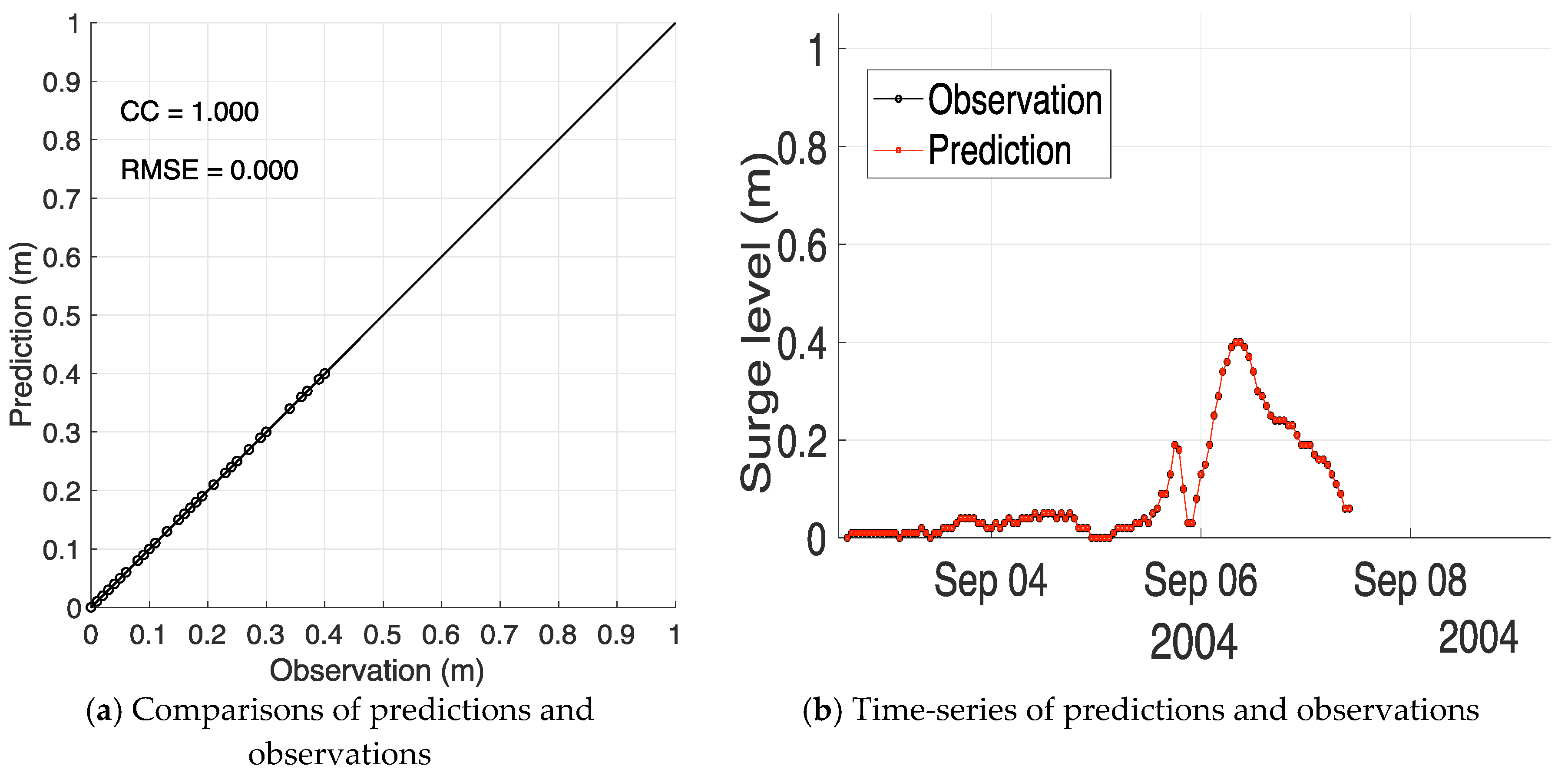
The additional experiment was carried out with the surge level in each combination. In this experiment, the GMDH-based storm surge models perfectly hindcasted the Songda surge level, except for model nos. 4, 8, 9, 10, and 21, which were not converged because the input data set formed singular matrices. One of the prediction results obtained from model no. 1 is given in Figure 5. As a result, the surge level highly impacted the prediction accuracy of the GMDH-based surge hindcast model.

3.2. Performances of GMDH-Based 5-h Lead Time Storm Surge Forecast Models

3.2.1. Exclusion of Surge Levels in the Training Data Set

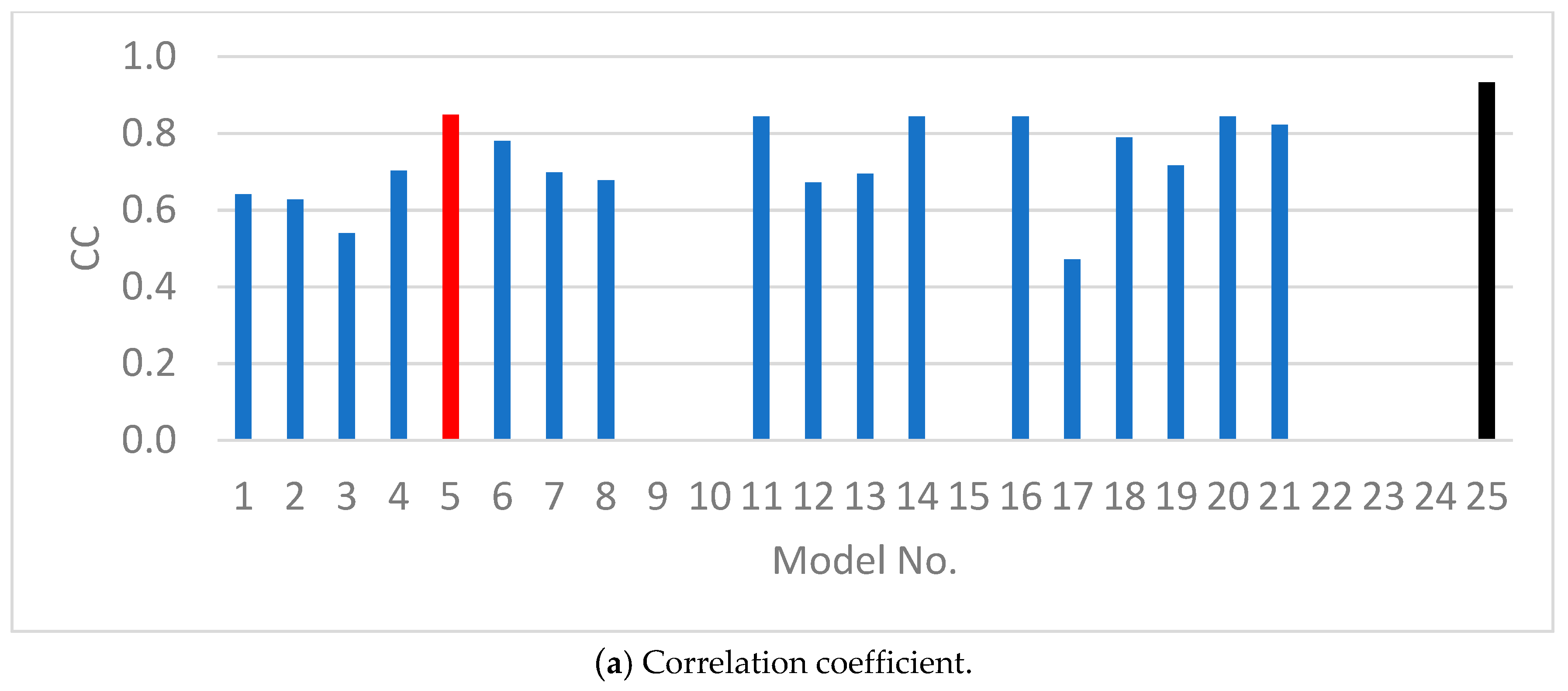
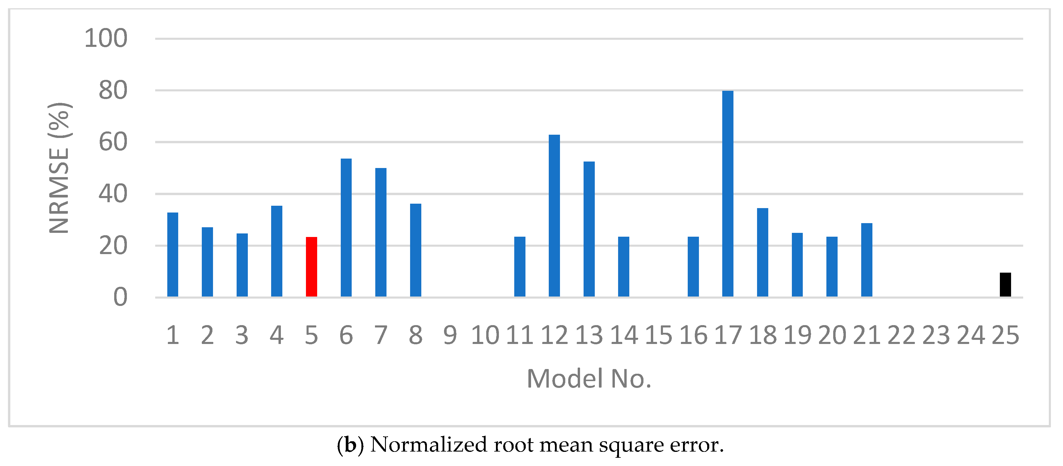
The GMDH-based 5-h lead time storm surge forecast models were trained with the data sets of Table 1. It ignored the surge level and was assessed with Typhoon Songda’s data in the testing phase. The averaged CC and NRMSE values were 0.78 and 10%, respectively. Among the models, the highest CC (0.881) was obtained from three models (see Figure 6a): model no. 4 was trained with SLP, DSLP, SSL, WS, and WD; model no. 12 was trained with SLP, DSLP, SSL, TP, and CP; model no. 17 was trained with SLP, DSLP, SSL, TP, CP, and MWS, which were identical to the training set of model no. 12, except for MWS. When comparing the CC values between model nos. 12 and 17, the parameter of MWS had no significant impact on the prediction of the Songda surge level. When comparing the CC value of model no. 4 with model nos. 1, 2, and 3, we found that the inclusion of sea surface level, wind speed, and wind direction benefits for predicting surge level and improving the CC value varied slightly. Furthermore, model no. 2 trained with SLP, DSLP, and SSL nearly had a similar CC value of 0.87. In other words, the parameters of sea-level pressure, drop rate, and sea surface level had a major effect on surge level prediction. In addition, the parameters of the typhoon position and its central pressure could have a minor impact, thus slightly improving prediction ability. On the other hand, the worst CC value was calculated from model no. 9 trained with SLP, DSLP, WS, WD, and TP. In comparison, with the CC of model no. 8 trained with the same data set to model no. 9 except for SSL, model no. 9′s CC became substantially worse. This was found when comparing other models with the CC of model no. 10, which was trained with the data set including SSL and excluding WS in the training set of model no. 9. The exclusion of WS had no significant impact on the prediction. Thus, for the 5-h lead time forecast, it can be said that the major parameters were sea-level pressure, drop rate, and sea surface level for training. The best model no. 12 was derived with the minimum least residual of 8.6%at the 4th layer through the development procedure described below:

$$y_4=0.00533+2.34286x_{4_4}-1.42545x_{7_4}+106.419x_{4_4}^2+99.754x_{7_4}^2-206.024x_{4_4}{x}_{7_4}$$

(33)

where $x_{4_4}$ and $x_{7_4}$ are the variables at the 4th hidden layer generated by a second-order polynomial derived at the 3rd hidden layer.

As shown Figure 6b, a trend of NRMSE was coherently similar to the trend of CC, wherein it is clear that the best CC and NRMSE are obtained from model nos. 4, 12, and 17, while the worst CC and NRMSE are acquired from model no. 9. On average, the value of NRMSE is approximately 10%. Model nos. 12 and 17 revealed 7.6% of NRMSE, which was the best. On the other hand, model no. 9 returned 22.9%, which was the worst and remarkable in comparison with other models’ accuracies.

Figure 7 shows comparisons between the observations and predictions of model no. 12. Surge levels were slightly overestimated from the beginning of the time-series. The GMDH-based model well predicted the first and second peaks. However, the model predicted the third peak next to the second one.

Kim et al. [24] reported that the training set that compounded the surge level, sea-level pressure, drop of sea-level pressure, longitude and latitude of typhoon’s location, sea surface level, and wind speed was the best (see model no. 25 in Figure 5). On the other hand, the current study’s best set consisted of sea-level pressure, drop rate, sea surface level, typhoon position, and central pressure. The parameters of sea-level pressure, drop rate, sea surface level, and typhoon position were in common, while the inclusion of the surge level and wind speed was incoherent. In other words, the cause of prediction accuracy might have come from the discrepancy in the training set. In particular, the surge level had a critical impact on the forecast accuracy. Both CC and NRMSE values obtained from model no. 25 were better than those from model no. 12. In addition, another possible reason is that that the two studies applied different neural network algorithms.

3.2.2. Inclusion of Surge Levels in the Training Data Set

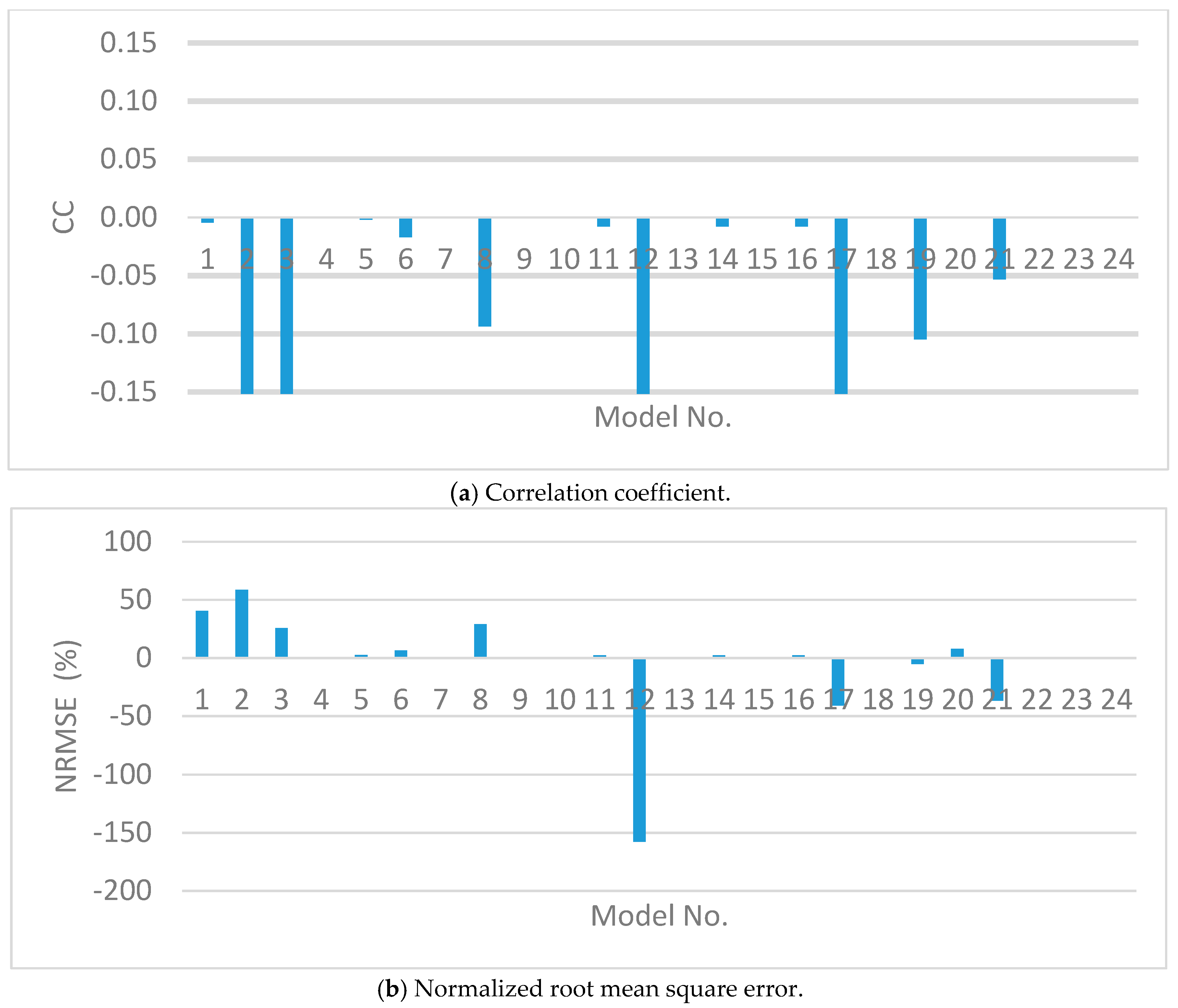
In the additional training, the surge level was included in each data set, as listed in Table 1. As shown in Figure 8, model nos. 7, 8, 9, 13, 15, 16, 21, and 23 were not converged with the data sets that included the surge level because a matrix of a data set was singular, resulting in an unsolvable inverse matrix. The GMDH-based 5-h lead time storm surge forecast models predicted the Songda surge with averaged CC and NRMSE to be0.83 and 18.03%, respectively. Compared to the values of 0.78 and 24.20% from the model trained without the surge level, the involvement of the surge level in the input data set deduced prediction accuracy improvement. On average, the improvement rates were 0.02 and 6% for CC and NRMSE, respectively. The improvement rates of CC (=(Surge − Nonsurge)/Nonsurge, where Surge and Nonsurge is the predicted surge level by the model trained by the data set with and without the surge level, respectively) and NRMSE (=(Nonsurge − Surge)/Nonsurge) are shown in Figure 9. The positive value indicates an improved surge level. The CC and NRMSE values were improved by 0.13 (model no. 5) and 34% (model no. 6). In this experiment, model no. 12 was selected as the best model because it had the smallest NRMSE and the second highest CC. In comparison, model no. 12 trained without the surge level and improved its NRMSE by 15%, although it incurred a slightly worse CC value of-0.04. As a result, the surge level was proven to be one of the key components for improving prediction accuracy.

Compared with the accuracy of the best ANN-based 5-h lead time storm surge forecast model (Kim et al. [24]), the GMDH-based model’s accuracy was lower (see model no. 25 in Figure 8). This value came from the characteristic differences of the two algorithms. For the practical application of the GMDH approach, the accuracy of the GMDH-based model should be improved by increasing the number of the typhoon.

3.3. Performances of GMDH-Based 12-h Lead Time Storm Surge Forecast Models

3.3.1. Exclusion of Surge Levels in the Training Data Set

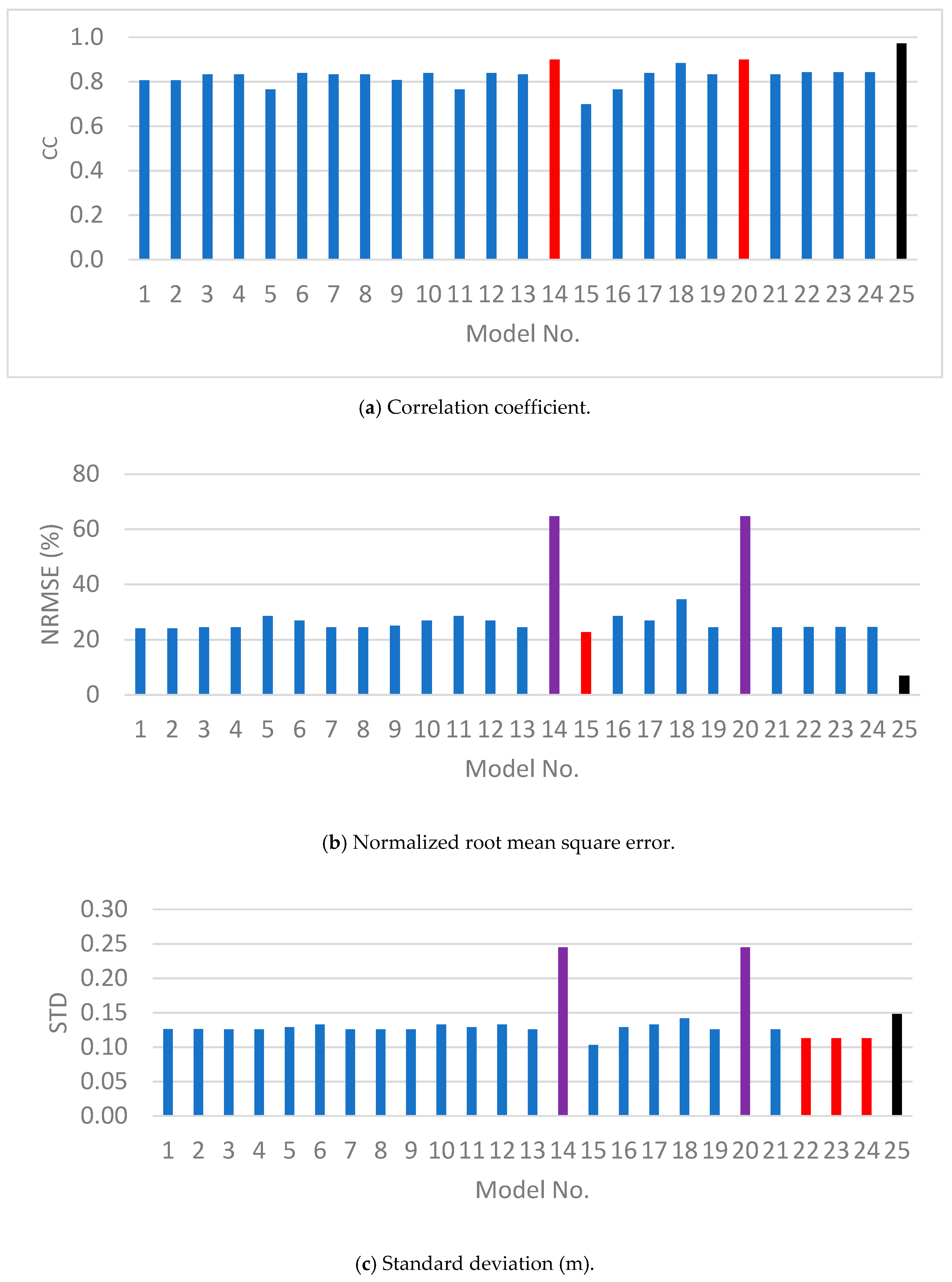
The testing results of the GMDH-based model are given in Figure 10. On average, the values of CC, NRMSE, and STD were 0.82, 12.2%, and 0.09 m, respectively. In this experiment, because CC and NRMSE were incoherent, STD was taken as an additional indicator. In CC, model nos. 14 and 20 were the highest. At the same time, NRMSE and STD indicated that the two models were the worst. When looking at the time-series of Songda’s surge, the models highly overestimated the surge levels around the peak (not shown here). This caused higher CCs and larger errors. On the other hand, model no. 15 had one of the smallest errors of NRMSE. However, a time-series in model no. 15 showed large time lags between observations and predictions (not shown here). Interestingly, all models except the model nos. 14, 20, 18, 16, 11, and 5 had a similar NRMSE order. Thus, we put our focus on STD, releasing the smallest one from model nos. 22, 23, and 24. These were trained with WS, WD, TP, and CP. Furthermore, three models predicted almost identical surge levels, as shown in Figure 11, implying that the training set of WS and WD was enough to train the GMDH-based storm surge forecast model with a 12-h lead time. However, the surge level predicted by the best models was highly amplified around the peak. As a result, the best model no. 22 was acquired with the lowest least residual of 0.046 (4.6%) after the 2nd iteration through the development procedure described as follows:

$$\begin{array}{c}{y}_2=0.0153805+0.153777x_{2_2}+0.599465x_{3_2}+3.76317x_{2_2}^2+1.04064x_{3_2}^2 \\ -4.40019x_{2_2}{x}_{3_2} \end{array}$$

(34)

where $x_{2_2}$ and $x_{3_2}$ are the variables at the 2nd hidden layer generated by a second-order polynomial derived at the 1st hidden layer.

In Kim et al. [24], the best training set was formed for the surge level, sea-level pressure, drop rate, and typhoon position (see model no. 25 in Figure 10). By including the surge level in the training set, the values of CC and NRMSE were improved, but STD was larger in comparison to the present result, which excluded it. However, the present result was not in line with Kim et al. [19]. It was believed that the reason that the current study did not include the surge level in the input training set was because the motivation of the study challenged the use of raw data observed at the station. Thus, the surge level should be calculated by extracting atmospheric tidal levels from the sea surface level. Further, because Kim et al. [19] did not test the best training set, which consisted of wind speed and wind direction, we were unable to directly compare the two results. One of the differences between the results of Kim et al. [24] and Hien et al. [26] was the implication of the different algorithms. We found that the storm surge time-series forecasted by model no. 22 was similar to those predicted by the support vector regression model presented by Hien et al. [26]. However, Figure 11 shows that the validation result of surge prediction was similar between the ANN-based model (Kim et al. [24]) and GMDH-based model in the present study. Therefore, further studies should be conducted to assess potential data sets that include surge levels, which improve forecast accuracy with a12-h lead time.

3.3.2. Inclusion of Surge Levels in the Training Data Set

In the previous experiment, the surge level was included in each data set. Some GMDH-derived equations were also not acquired because of the singular matrix (see Figure 12), i.e., model nos. 3, 4, 7, 8, 15, 19, and 21. Among the GMDH-based models, model nos. 14 and 20 were the best models because it had the highest CC (Figure 12a), while model no. 13 was the best because it had the lowest NRMSE (Figure 12b). In addition, when the surge level was included, model nos. 2 and 6were not improved for CC (Figure 13a) and model nos. 1, 2, and 6 were not improved for NRMSE (Figure 13b). The rest of the models, however, were either improved or remained exactly the same in comparison to the models trained with the data set, including surge level. The averaged CC and NRMSE were 0.83 and 26.3%, whereas for the surge level they were 0.83 and 29.05%. In other words, the surge level in the input data set and GMDH-based model’s NRMSE was improved. When excluding the surge level, the best model was model no. 22, which was trained with the WS, WD, TP, and CP data sets. However, when the surge level was included in the input layer, model nos. 14 and 20 demonstrated improved accuracy. Further, CC values became slightly better, ranging from 0.9 to 0.91, while NRMSE changed from 65% to 26%. As mentioned above, the best models were model nos. 14 and 20, which had the largest CC and smallest NRMSE. This was determined by considering the surge level in the SLP, DSLP, WS, WD, TP, CP, and MWS data sets.

Although the GMDH-based model was trained with a data set that included the surge level, the GMDH-based 12-h lead time surge forecast model was unable to be more accurate than the ANN-based 12-h lead time surge forecast model (see model no. 25 in Figure 12).

3.4. Performances of GMDH-Based 24-h Lead Time Storm Surge Forecast Models

3.4.1. Exclusion of Surge Levels in the Training Data Set

Figure 14 depicts the performance indices of CC, NRMSE, and STD. The averaged indices were 0.79, 15.1%, and 0.08 m for CC, NRMSE, and STD, respectively. Among the 24 models, the highest CC values of 0.87 were calculated from model nos. 12 and 21, while the lowest NRMSE of 8% came from model no. 21. Model nos. 1 and 2 presented the worst CC (0.64) and NRMSE (27.5%), respectively. The STD value also indicated that model no.21 had the smallest error of 0.04 m. As a result, the best performance for model no. 21 could be obtained, when training with the SLP, DSLP, SSL, WS, WD, TP, CP, and MWS data sets. Kim et al. [24] showed that the best training set compounds of the surge level were SLP, DSLP, WS, WD, and TP (see model no. 25 in Figure 14). Although the surge level was not taken as an input parameter in this study, model no. 8 was trained with the same parameter set as in Kim et al. [24]’s best set, except for the surge level, which revealed large errors in comparison to model no. 21. This could be a result of the surge level being the input layer and a vital factor for predicting surge level with the lead time. When comparing model nos. 12 and 21, the wind speed, wind direction, and maximum wind speed were thought to improve model prediction error. Of the worse performance models, model nos. 1 and 2 were trained with seal-level pressure, drop rate, and sea surface level, each of which significantly revealed more substantial CC, NRMSE, and STD errors. In other words, the too-small number of the input parameter caused an inaccurate prediction. Figure 9 show son the right side along the x-axis that the errors of NRMSE and STD became small. As a result, model no. 21 was secured with the lowest least residual of 0.032 (3.2%) in the 2nd iteration:

$$\begin{array}{c}{y}_2=0.029+0.173109x_{3_2}-0.186717x_{{25}_2}-0.978694x_{3_2}^2+0.596642x_{{25}_2}^2\\ +5.26692x_{3_2}{x}_{{25}_2}\end{array}$$

(35)

where $x_{3_2}$ and $x_{{25}_2}$ are the variables at the 2nd hidden layer generated by a second-order polynomial derived at the 1st hidden layer.

Figure 15 depicts comparisons of observations and predictions. Overall, the best 24-h lead time forecast model overestimated the Songdasurge level. While the peak level was well predicted, the surge levels around the first peak and after the second peak were overestimated. Compared with the ANN results in Kim et al. ([24,25]) and GP results in Hien et al. [26], we found that the accuracy of the best GMDH-based model was closer to the results obtained from the deterministic data-driven models, i.e., the multi-layer perceptron, k-nearest neighbors, decision tree, and support vector regression, as shown in Hien et al. [26]. As mentioned above, the surge level was omitted in the present study, which may have had an impact on surge prediction.

3.4.2. Inclusion of Surge Levels in the Training Data Set

The additional experiment investigated the effect of the surge level on prediction accuracy of the 24-h lead time by including the surge level in the data set. As found from previous experiments, some GMDH-based models did not converge (i.e., model nos. 9, 10, 15, 22, 23, and 24) (Figure 16). The CC and NRMSE values obtained from models trained by the data set without the surge level were 0.79 and 36% on average. On the other hand, those from the models trained by the data set with the surge level were 0.73 and 36.64% on average. Overall, the CC of the models was similar or worse when the surge level was involved (see Figure 17a). Furthermore, when the input data was small, the improvement of the prediction accuracy (NRMSE) was apparent (see model nos. 1, 2, 3, and 8 in Figure 17b). When comparing the improvement rates of the 5 and 12-h lead times, the improvement rate apparently declined during the 24-h lead time. In other words, the effect of the surge level on the 24-h lead time forecast accuracy was not critical. Among the GMDH-based models, model no. 5 showed the best performance based on CC and NRMSE values. However, model no. 21 trained without the surge level was more accurate than model no. 5 trained with the surge level.

In addition, the accuracy of the GMDH-based 24-h lead time storm surge forecast model trained with the data set including the surge level did not reach the ANN-based 24-h lead time storm surge forecast model (see Figure 16).

4. Discussion

Sakaiminato’s storm surge has peak level characteristics that appear approximately 15 h after a typhoon’s passage. In addition, typhoon’s move offshore without landfall. The annual tidal range is approximately 0.3 m on average. We found that the best training data set compounds the site-specific typhoon-related component, depending on the lead time through the experiment. In the experiment that excluded surge level for the zero-hour lead time, the surge was generated via sea-level pressure, drop rate, wind speed, and wind direction after the typhoon passed offshore. When the surge was forecasted with the 5-h lead time, the indicators of the typhoon position and central pressure were necessary. The 12 h almost corresponded to the time of the peak surge level occurrence and was a time when the typhoon was located around Hokkaido Prefecture, which is more than 800 km away from Sakaiminato. Therefore, wind information should be added as an indicator. The Ekman setup led by Ekman transport was a component of wind-driven ocean currents that generatedanafter-runner storm surge at Sakaiminato in the presence of the Coriolis force over the Tottori coast (Kim et al. [2]). The 24-h lead time affected non-stormy weather and the ocean, resulting in arequirement of all the typhoon-related components. In the additional experiment where the data set included the surge level, we found that the surge level improved the near–far forecast’s prediction accuracy. However, we still need to further investigate the feature selection because we missed several combinations, i.e., eight components of the 28 data sets. Therefore, a feature selection that automatically decides critical components without making potential combinations should be proposed.

Through the methodology presented in this study, it was clear that the GMDH enabled application to other sites. Thus, site-specific typhoon-related characteristics were assessed by the feature selection and the storm surge forecast model was developed by training with fully large data that could be produced via numerical simulations using long-term ensemble projections for historical and future climates (e.g., Mori et al. [33]) and stochastic tropical cyclone models (e.g., Nakajo et al. [41]).

Even though the number of typhoons considered in the current study was small, they were still sufficient indemonstrating GMD Heffectiveness. The three typhoons generated sufficiently high surge levels that corresponded to a 100-year return period at Sakaiminato. Those typhoons can be treated ashistorically representative because they generate after-runner storm surges and record winds and pressures at local meteorological stations. However, the present study did not consider potential typhoons that generated either high or lowsurge levels, at least compared with the three typhoon-generated surge levels thatresulted in potential forecast errors. Therefore, the typhoon number should increase for practical forecasting. In addition to the typhoon number, Mori et al. [33] reported that the future 100-year return values of storm surge would increase by 20% on the East Asian coast due to climate change. From this perspective, we expect that the storm surge at Sakaiminato will increase by approximately 0.6 m in the future. Therefore, climate change’s impact should be considered when training the GMDH-based surge forecast model with experimental climate change data. Once the GMDH-based storm surge forecast model is successively trained, the storm surge forecast model with an ensemble prediction system (EPS) can estimate the uncertainty in a storm surge forecast. Therefore, the accuracy of the GMDH-based forecast model with EPS should be assessed in practice. Suppose its accuracy is satisfied with uncertainty. In that case, the GMDH-based forecast model could provide arrange of surge levels using typhoon information forecasted with JMA and observations at designated time intervals. Thus, the forecasted surge levels can serve as a pre-indicator for evacuation.

The performance of the GMDH-based surge forecast model is highly relevant to the reliability of the present method. Hien et al. [25] compared machine learning methods that resulted in better GP and ANN stochastic methods performances, especially in comparison with multi-layer perceptron, k-nearest neighbors, decision tree, and support vector regression, which are ordinarily called data-driven models, as they can capture the mapping between input and output variables (forecast problems) without directly studying the mechanism of storm surges. The GMDH is one of these stochastic methods and thus has better reliability than the data-driven method. However, the present method used GMDH results with lower accuracy, as compared to the ANN and GP methods (Kim et al. [24], Hien et al. [26]). Moreover, the present method either included or excluded the surge level in data set results with higher accuracies for the 5- and 12-h lead times, and the same accuracy for the 24-h lead time. In other words, the accuracy of the present GMDH method can be improved with an appropriate training set and data set, as described above.

5. Conclusions

The present study developed a storm surge forecast model for Sakaiminato, Tottori, Japan using the GMDH algorithm. The study challenged forecast storm surge levels with lead times of 5, 12, and 24 h, and then hind casted them. To train the GMDH-based model, local meteorological and hydrodynamic data was observed and collected at stations around Sakaiminato during Typhoons Maemi (2003), Songda (2004), and Megi (2004). In the forecast experiments, we used two typhoons—Maemi and Megi—and one typhoon (Songda) for training and testing, respectively. The present study’s remarkable conclusions are presented below:

• For training the GMDH-based hind cast model, the best training set can be made by adding the surge level to other components.
• The best set consisted of the surge level, sea-level pressure, drop rate, sea surface level, typhoon position, and central pressure, all of which resulted in the most accurate GMDH-based 5-h lead time forecast model.
• The surge level, wind speed, and wind direction are required for the best set of GMDH-based 12-h lead time forecast model.
• To forecast the surge level with a 24-h lead time, many types of input parameters are preferable, and all input parameters were shown in this study.
• The inclusion of the storm surge level at the input layer is critical to the accuracy of the near–far forecast model for the 5- and 12-h lead times, particularly.

Further studies should be done with large data sets to consider climate change and to improve the accuracy of the GMDH-based storm surge forecast model. Moreover, the uncertainty of the GMDH-based storm surge forecast model with an ensemble prediction system should be verified for the practical forecast. Furthermore, a selection procedure to automatically decide components should be investigated against other man-made data sets.

References

- Publisher’s Note: MDPI stays neutral with regard to jurisdictional claims in published maps and institutional affiliations.
- Mori, N.; Yasuda, T.; Arikawa, T.; Kataoka, T.; Nakajo, S.; Suzuki, K.; Yamanaka, Y.; Webb, A. 2018 Typhoon Jebi post-event survey of coastal damage in the Kansai region, Japan. Coast. Eng. J. 2019, 61, 278–294. [Google Scholar]
- Kim, S.; Matsumi, Y.; Yasuda, T.; Mase, H. Storm surges along the Tottori coasts following a typhoon. Ocean Eng. 2014, 91, 133–145. [Google Scholar] [CrossRef]
- Hiyajo, H.; Okubo, S.; Takasa, S.; Kobashigawa, Y.; Nishimura, F.; Toomine, T.; Daimon, H.; Itagaki, S.; Fukuda, M.; Sakaji, T.; et al. Digitizing the Historical Sea Level Data and Re-Analysis of Storm Surges with the Data. Meteorol. Bull. Jpn Meteorol. Agency 2011, 78, S1–S32. Available online: http://www.jma.go.jp/jma/kishou/books/sokkou-kaiyou/78/vol78s001.pdf (accessed on 10 October 2020). (In Japanese).
- Jelesnianski, C.P.; Chen, J.; Shaffer, W.A. SLOSH: Sea, lake, and overland surges from hurricanes, NOAA Technical Report. NWS-48; U.S. Department of Commerce, National Oceanic and Atmospheric Administration, National Weather Service: Silver Spring, MD, USA, 1992; p. 71. [Google Scholar]
- Luettich, R.A.; Westerink, J.J. Formulation and Numerical Implementation of the 2D/3D ADCIRC Finite Element Model Version 44. 2004. Available online: https://adcirc.org/files/2018/11/adcirc_theory_2004_12_08.pdf (accessed on 10 October 2020).
- Chen, C.; Beardsley, R.C.; Cowles, G. An unstructured grid, finite-volume coastal ocean model (FVCOM) system. Special Issue entitled “Advance in Computational Oceanography”. Oceanography 2006, 19, 78–89. [Google Scholar]
- Zhang, Y.; Baptista, A.M. SELFE: A semi-implicit Eulerian–Lagrangian finite-element model for cross-scale ocean circulation. Ocean Modell. 2008, 21, 71–96. [Google Scholar]
- Delft3D-FLOW User Manual: Simulation of multi-dimensional hydrodynamic flows and transport phenomena, including sediments. Technical Report; Version: 3.15, Revision 36209; Deltares: Delft, The Netherlands, 2014; p. 686. Available online: https://oss.deltares.nl/documents/183920/185723/Delft3D-FLOW_User_Manual.pdf (accessed on 10 October 2020).
- Sooyoul Kim Yasuda, T.; Mase, H. Effects of Tidal Variations on Storm Surges and Waves. Appl. Ocean Res. 2008, 30, 311–322. [Google Scholar]
- Kim, S.; Hara, C.; Kurahara, Y.; Nishiyama, Y.; Takeda, M.; Tom HATKawasaki, K.; Mase, H. Application of GMDH-based one week wave prediction model to Japanese near shore wave prediction. J. Jpn. Soc. Civ. Eng. Ser. B2 (Coast. Eng.) 2019, 75, I_115–I_120. [Google Scholar]
- Deo, M.C.; Sridhar, N.C. Real time wave forecasting using neural networks. Ocean Eng. 1999, 26, 191–203. [Google Scholar]
- Deo, M.C.; Jha, A.; Chaphekar, A.; Ravikant, K. Neural networks for wave forecasting. Ocean Eng. 2001, 28, 889–898. [Google Scholar]
- Londhe, S.; Panchang, V. One-day wave forecasts based on artificial neural networks. J. Atmos. Ocean. Technol. 2006, 23, 1593–1603. [Google Scholar]
- Makarynskyy, O.; Pires-Silva, A.; Makarynska, D.; Ventura-Soares, C. Artificial neural networks in wave predictions at the west coast of Portugal. Comput. Geosci. 2005, 31, 415–424. [Google Scholar]
- Oh, J.; Suh, K.-D. Real-time forecasting of wave heights using EOF–wavelet–neural network hybrid mode. Ocean Eng. 2018, 150, 48–59. [Google Scholar] [CrossRef]
- James, S.C.; Zhang, Y.; O’Donncha, F. A machine learning framework to forecast wave conditions. Coast. Eng. 2018, 137, 1–10. [Google Scholar] [CrossRef] [Green Version]
- Tom, T.H.A.; Mase, H.; Ikemoto, A.; Saitoh, T.; Kawasaki, K.; Takeda, M. Wave Prediction by neural network using atmospheric pressure and wind speeds. J. Japan Soc. Civ. Eng. Ser. B2 (Coast. Eng.) 2018, 74, I_691–I_696. [Google Scholar]
- Tsai, C.C.; Wei, C.C.; Hou, T.H.; Hsu, T.-W. Artificial neural network for forecasting wave weights along a ship’s route during hurricanes. J. Waterw. Port Coast. Ocean Eng. 2018, 144, 04017042. [Google Scholar] [CrossRef]
- Tsuda, M.; Matsumi, Y.; Kim, S.; Matsuda, N.; Eguchi, M. Wave forecasts using an artificial neural network for port construction management. J. Jpn. Soc. Civ. Eng. Ser. B2 (Coastal Eng.) 2017, 73, I_151–I_156. [Google Scholar] [CrossRef] [Green Version]
- Lee, S.B.; Suh, K.-D. Development of wave overtopping formulas for inclined seawalls using GMDH Algorithm. KSCE J. Civ. Eng. 2019, 1–12. [Google Scholar] [CrossRef]
- Mase, H.; Kitano, T. Prediction model for occurrence of impact wave force. Ocean Eng. 1999, 26, 949–961. [Google Scholar]
- Mase, H.; Sakamoto, M.; Sakai, T. Neural network for stability analysis of rubble-mound breakwaters. J. Waterw. Port Coast. Ocean Eng. 1995, 121, 294–299. [Google Scholar]
- Van Gent, M.R.A.; van den Boogaard, H.F.P. Neural network modeling of forces on vertical structures. Coastal Eng. 1998, 2096–2109. [Google Scholar]
- Kim, S.; Matsumi, Y.; Pan, S.; Mase, H. A real-time forecast model using artificial neural network for after-runner storm surges on the Tottori coast, Japan. Ocean Eng. 2016, 122, 44–53. [Google Scholar]
- Kim, S.; Pan, S.; Mase, H. Artificial neural network-based storm surge forecast model: Practical application to Sakai Minato, Japan. Appl. Ocean Res. 2019, 91, 101871. [Google Scholar] [CrossRef]
- Hien, N.T.; Tran, C.T.; Nguyen, X.H.; Kim, S.; Phai, V.D.; Thuy, N.B.; Van Manh, N. Genetic Programming for Storm Surge Forecasting. Ocean Eng. 2020, 215, 107812. [Google Scholar] [CrossRef]
- Sahoo, B.; Bhaskaran, P.K. Prediction of storm surge and inundation using climatological datasets for the Indian coast using soft computing techniques. Soft Comput. 2019, 23, 12363–12383. [Google Scholar]
- De Oliveira, M.M.; Ebecken, N.F.F.; De Oliveira, J.L.F.; de Azevedo Santos, I. Neural network model to predict a storm surge. J. Appl. Meteorol. Climatol. 2009, 48, 143–155. [Google Scholar]
- Lee, T.-L. Prediction of storm surge and surge deviation using a neural network. J Coast. Res. 2008, 24, 76–82. [Google Scholar]
- Deo, M.C.; Chaudhar, G. Tide prediction using neural networks. Comput. Aided Civ. Infrastruct. 1998, 13, 113–120. [Google Scholar]
- Yoon, H.-D.; Cox, D.T.; Kim, M. Prediction of time-dependent sediment suspension in the surf zone using artificial neural network. Coast. Eng. 2013, 71, 78–86. [Google Scholar] [CrossRef]
- Chang, T.C.; Chao, R.J. Application of back-propagation networks in debris flow prediction. Eng. Geol. 2006, 85, 270–280. [Google Scholar]
- Mori, N.; Shimura, T.; Yoshida, K.; Mizuta, R.; Okada, Y.; Fujita, M.; Khujanazarov, T.; Nakakita, E. Future changes in extreme storm surges based on mega-ensemble projection using 60-km resolution atmospheric global circulation model. Coast. Eng. J. 2019, 61, 295–307. [Google Scholar] [CrossRef] [Green Version]
- Roberts, K.J.; Colle, B.A.; Georgas, N.; Munch, S.B. A regression-based approach for cool-season storm surge predictions along the New York-New Jersey Coast. J. Appl. Meteorol. Climatol. 2015, 54, 1773–1791. [Google Scholar] [CrossRef]
- Koza, J.R. Genetic Programming: On the Programming of Computers by Means of Natural Selection, 1st ed.; A Bradford Book; The MIT Press: Cambridge, MA, USA; London, UK, 1992; p. 840. [Google Scholar]
- Kondo, T. GMDH-type neural network algorithm self-selecting optimum neural network architecture and its application to medical image recognition. IEICE Tech. Rep. Theor. Found. Comput. 2008, 108, 17–24. [Google Scholar]
- Mo, L.; Xie, L.; Jiang, X.; Teng, G.; Xu, L.; Xiao, J. GMDH-based hybrid model for container throughput forecasting: Selective combination forecasting in nonlinear subseries. Appl. Soft Comput. 2018, 62, 478–490. [Google Scholar]
- Ivakhnenko, A.G. Polynomial theory of complex systems. IEEE Trans. Syst. Man Cybern. 1971, 1, 364–378. [Google Scholar]
- Onwubolu, G. Hybrid Self-Organizing Modeling; Springer: Berlin/Heidelberg, Germany, 2009; p. 297. [Google Scholar]
- Flowerdew, J.; Horsburgh, K.; Wilson, C.; Mylne, K. Development and evaluation of an ensemble forecasting system for coastal storm surges. Q. J. R. Meteorol. Soc. 2010, 136, 1444–1456. [Google Scholar] [CrossRef] [Green Version]
- Nakajo, S.; Mori, N.; Yasuda, T.; Mase, H. Global Stochastic Tropical Cyclone Model Based on Principal Component Analysis and Cluster Analysis. J. Appl. Meteor. Climatol. 2014, 53, 1547–1577. [Google Scholar] [CrossRef]
Figure 1.
Typhoon tracks and stations for meteorological (Hamada, Yonago, Matsue, Ama, and Saigo) and hydrodynamic (Sakaiminato) stations around Sakaiminato, Tottori, Japan.
Figure 2.
A procedure that develops the group method of data handling (GMDH)-based storm surge forecast model (circle indicates the element).
Figure 3.
Performance indices of CC and NRMSE were calculated between Typhoon Songdasurge levels observed at Sakaiminato and hindcasted by the GMDH-based storm surge hindcast models. Red indicates the highest CC (or the lowest NRMSE), while purple shows the worst.
Figure 4.
Comparisons of observations and predictions hindcasted by model no. 4, which was the best performance model at Sakaiminato.
Figure 5.
Comparisons of observations and predictions hindcasted by model no.1 at Sakaiminato.
Figure 6.
Performance indices of CC and NRMSE calculated between Typhoon Songda surge levels observed at Sakaiminato and predicted by the GMDH-based 5-h lead time storm surge forecast models. Model no. 25 is the best 05-h lead time ANN-based model trained by the input data set consisting of the surge level, sea-level pressure, drop of sea-level pressure, longitude and latitude of typhoon, sea surface level, and wind speed (Kim et al. [24]).
Figure 7.
Comparisons of observations and predictions forecasted by model no.12, which is the best for the 5 h-lead time at Sakaiminato.
Figure 8.
Performance indices of CC and NRMSE calculated between Typhoon Songda surge levels observed at Sakaiminato and predicted by the GMDH-based 5-h lead time storm surge forecast models trained with the data set that included the surge level. Model no. 25 is the best 05-h lead time ANN-based model trained by the input data set consisting of surge level, sea-level pressure, drop of sea-level pressure, longitude and latitude of typhoon, sea surface level, and wind speed (Kim et al. [24]).
Figure 9.
Improvement rates of the inclusion of surge level in the input data set to the exclusion for CC and NRMSE, respectively. For CC and NRMSE, positive means that the inclusion of the surge level improved.
Figure 10.
Performance indices of CC and NRMSE calculated between Typhoon Songda surge levels observed at Sakaiminato and predicted by the GMDH-based 12-h lead time storm surge forecast models. Model no. 25 is the best ANN-based 12-h lead time model trained by the input data set that consisted of surge level, sea-level pressure, drop of sea-level pressure, longitude and latitude of typhoon, sea surface level, and wind speed (Kim et al. [24]).
Figure 11.
Comparisons of observations and predictions forecasted by model no. 22 that is the best performance model for the 12-h lead time at Sakaiminato.
Figure 12.
Figure 13.
Figure 14.
Performance indices of CC and NRMSE calculated between Typhoon Songda surge levels observed at Sakaiminato and predicted by the GMDH-based 24-h lead time storm surge forecast models. Model no. 25 is the best ANN-based 24-h lead time model trained by the input data set that consisted of surge level, sea-level pressure, drop of sea-level pressure, longitude and latitude of typhoon, sea surface level, and wind speed (Kim et al. [24]).
Figure 15.
Comparisons of observations and predictions forecasted by model no. 21, which is the best for the 24 h-lead time at Sakaiminato.
Figure 16.
Performance indices of CC and NRMSE
calculated between Typhoon Songda surge levels observed at Sakaiminato and
predicted by the GMDH-based 24-h lead time storm surge forecast models. Model
no. 25 is the best ANN-based 24-h lead time model trained by the input data set
that consisted of surge level, sea-level pressure, drop of sea-level pressure,
longitude and latitude of typhoon, sea surface level, wind direction, and wind
speed (Kim et al. [24]).
Figure 17.