3D Numerical Simulations of Green Water Impact on Forward-Speed Wigley Hull Using Open Source Codes

1
School of Naval Architecture and Ocean Engineering, Jiangsu University of Science and Technology, Zhenjiang 212000, China
2
China Ship Scientific Research Center, Wuxi 214082, China
*
Author to whom correspondence should be addressed.
J. Mar. Sci. Eng. 2020, 8(5), 327; https://doi.org/10.3390/jmse8050327
Submission received: 19 March 2020
/
Revised: 27 April 2020
/
Accepted: 28 April 2020
/
Published: 6 May 2020
(This article belongs to the Special Issue Ship Dynamics for Performance Based Design and Risk Averse Operations)
Abstract
:A series of CFD RANS simulations are presented for Wigley hulls of two freeboard heights progressing with forward speed in waves. Free surface effects are captured using the Volume of Fluid (VOF) method embedded in open source software OpenFOAM. Comparisons of heave, pitch motions and added resistance of the first Wigley model against the experiments of Kashiwagi (2013) confirm the numerical validity of the hydrodynamic modelling approach. Further simulations for the lower-freeboard Wigley model reveal that the highest green water impact on decks appears in way of and at the highest instantaneous pitch amplitude where the water propagates far downstream and across the deck. The simulations also demonstrate that the green water events are associated with air bubble entrapment.
1. Introduction
Under harsh sea conditions, vessels or offshore platforms endure large wave loads, such as bottom and bow slamming, green water on decks, etc. Severe slamming may lead to serious structural damage and may affect the safety and stability of the vessel or offshore platform. Green water may not pose a direct threat to integrity or survivability but may result in increasing expenses for repairs and renewal of damaged topside modules or outfitting equipment [1,2].
Over the years the development of non linear numerical methods for the assessment of risks associated with impact of green water on decks has been challenging. Measuring freeboard exceedance or free surface elevation relative to the deck using 3D linear diffraction theory has been extensively applied for the prediction and statistical analysis of green water risk due to its relative simplicity [3,4,5]. In reality, a green water event is highly nonlinear. This implies that linear potential flow theory and the assumption of a Rayleigh distribution for the statistics may be inaccurate [3,6,7,8,9].
Another method used is the so-called composite method. In this numerical idealisation the green water event is divided into four different stages and each of them is modeled separately using distinct methodologies. The freeboard exceedance is used as input for a dam-break model [10,11,12,13,14] or as a solution to the shallow water equations [15,16] that can simulate hydrodynamic behaviour of on-deck flows. The green water loading on deck structures is approximated either analytically by the similarity method [17] and Wagner-type analysis [18] or empirically by utilizing extensive scale model tests [3]. Computational Fluid Dynamics (CFD) is then adopted to idealise the influence of local fluid flow in way of the localized regions around the bow or to simulate local interactions between green water flows and deck structures [3,19,20]. Uncertainties associated with modeling assumptions constrain the accuracy of this method that, in any case, could be considered more suitable for preliminary design stage.
With the successful development of high performance computing, CFD simulations using the volume of fluid (VOF) method may be considered as a valuable alternative [2,21,22,23,24,25,26,27,28]. However, to capture the nonlinear evolution of wave groups and wave-structure interactions, high mesh resolution is required in such simulations. For example, for the simulation of green water events, finer mesh is required to accommodate for the influence of shallow water hydrodynamics on deck.
This paper presents a series of CFD RANS simulations for Wigley hulls of two freeboard heights progressing with forward speed in waves. Free surface effects are captured using the Volume of Fluid (VOF) method embedded in open source software OpenFOAM. Heave, pitch motions and added resistance of the first Wigley hull model are compared against the experiments of Kashiwagi (2013) [29]. Pressures on the deck bow of the lower-freeboard Wigley hull model are measured and flow observations of green water are carried out. The study provides complementary understanding of green water dynamics on deck and key physics of the green water events.
2. Mathematical Model and Numerical Method
The flow is governed by the incompressible Navier–Stokes equations
where (, 2, 3) denotes flow velocity at the x-, y- and z-axes respectively, represents the mixture density of the two phases separately considered, p denotes pressure, is dynamic viscosity of the fluid, g represents the gravitational acceleration.
A Reynolds averaging approach is adopted to smear out the fluctuating components of the solution variables in the instantaneous Navier–Stokes equations so as to alleviate the computational cost. Averaging the continuity and Navier–Stokes equations yields
where and represent the ensemble-averaged velocity and pressure; the product denotes the Reynolds stress component. Thereafter Reynolds-averaged Navier–Stokes (RANS) equations govern the transport of flow. The Reynolds stress in Equation (4) is modeled as a function of turbulent viscosity and the mean velocity gradients according to Boussinesq hypothesis
where k is is the turbulent kinetic energy and is the Kronecker delta.
To obtain the turbulent viscosity, the shear-stress transport (SST) k- two-equation model proposed by Menter [30] is used as follows
where represents the specific dissipation rate,
and and are the blending functions [30].
The volume of fluid (VOF) method with artificial bounded compression technique proposed by Hirt and Nichols (1981) [31] was used to capture the free surface. The free surface was considered as a mixture of water and air and accordingly the VOF transport equation was expressed as
where is the relative velocity between the water and air and termed as “compression velocity”; represents the volume fraction defined as the relative volume proportion of water in a cell, namely
The spatial variation of fluid density and dynamic viscosity can be then expressed as
where the subscripts “water” and “air” represent the corresponding fluid property of water and air respectively.
Rigid body motion equations, in which all other motions are constrained apart from heave and pitch, were used to model the dynamic response of the ship as follows
where m denotes the ship mass; z is displacement in heave; represents the total force in the vertical direction; denotes moment of inertia in pitch; represents angle in pitch, N is moment of force in pitch. The Newmark- method [32] with and was used to solve Equations (13) and (14).
Mesh deformation was achieved by moving the node points of the mesh according to the ship motion and without changing the mesh topology. The displacements of the node points were then calculated by using the equation
where represents the displacements of the node points; r denotes the distance of the cell centre to the nearest moving wall boundary.
3. Problem Setup
At first instance Equation (9) was solved for a fraction of volume and then integrated across the entire flow field. Then, the Reynolds-averaged Navier–Stokes equations using the SST model were solved by the OpenFOAM interFoam subroutine as follows
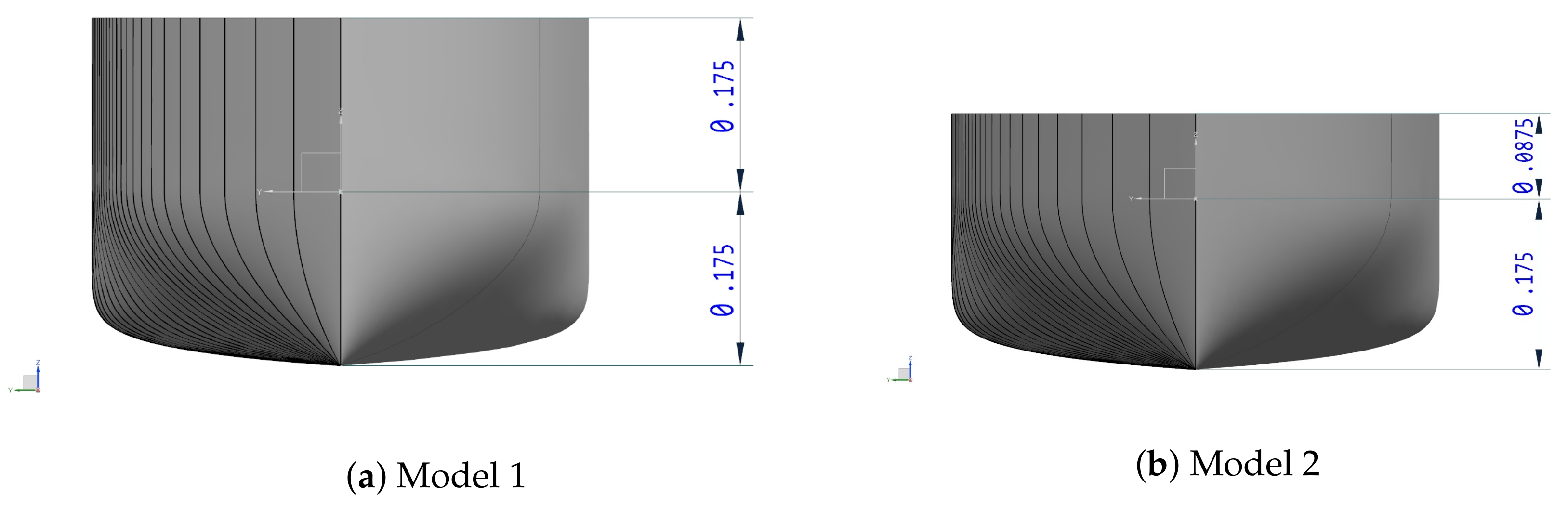
where B denotes the waterline breadth; L denotes the length between perpendiculars; d represents the draft. To observe the green water occurrence, two blunt Wigley hull models with different freeboard heights were considered (see Figure 1 and Table 1).
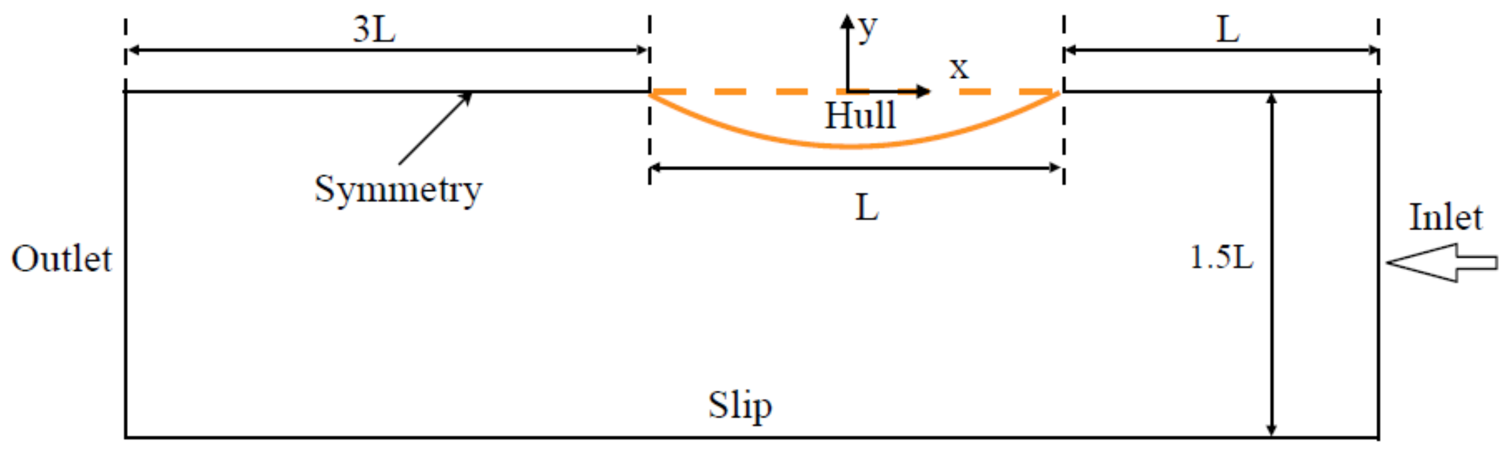
A top view of the layout of the computational domain according to Chen et al. (2019) [2] is shown in Figure 2. The first-order Stokes regular head wave was generated in the wave tank for Froude number () of 0.2. Assuming that the wave propagates along the negative x-axis direction, the wave elevation , the encounter frequency and the incident wave potential were written as
the velocity components of the water were then defined as follows
where A represents the wave amplitude; k is the wave number; denotes the natural frequency; U represents the ship speed; H is the water depth.
For all cases, the free surface was set at with the draft . Equations (20)–(22) were then used to define the boundary condition at the inlet. At the outlet, a damping zone of wave length was set to damp the vertical motions of an interface by applying a force () to the momentum equation proportional to the momentum of the flow in the direction of gravity. Fluid damping effects lead to exponential decay of the vertical velocity (), where is set based on the desired level of damping and the residence time of a perturbation through the damping zone. At the mid plane of the hull, a symmetry boundary condition was used.
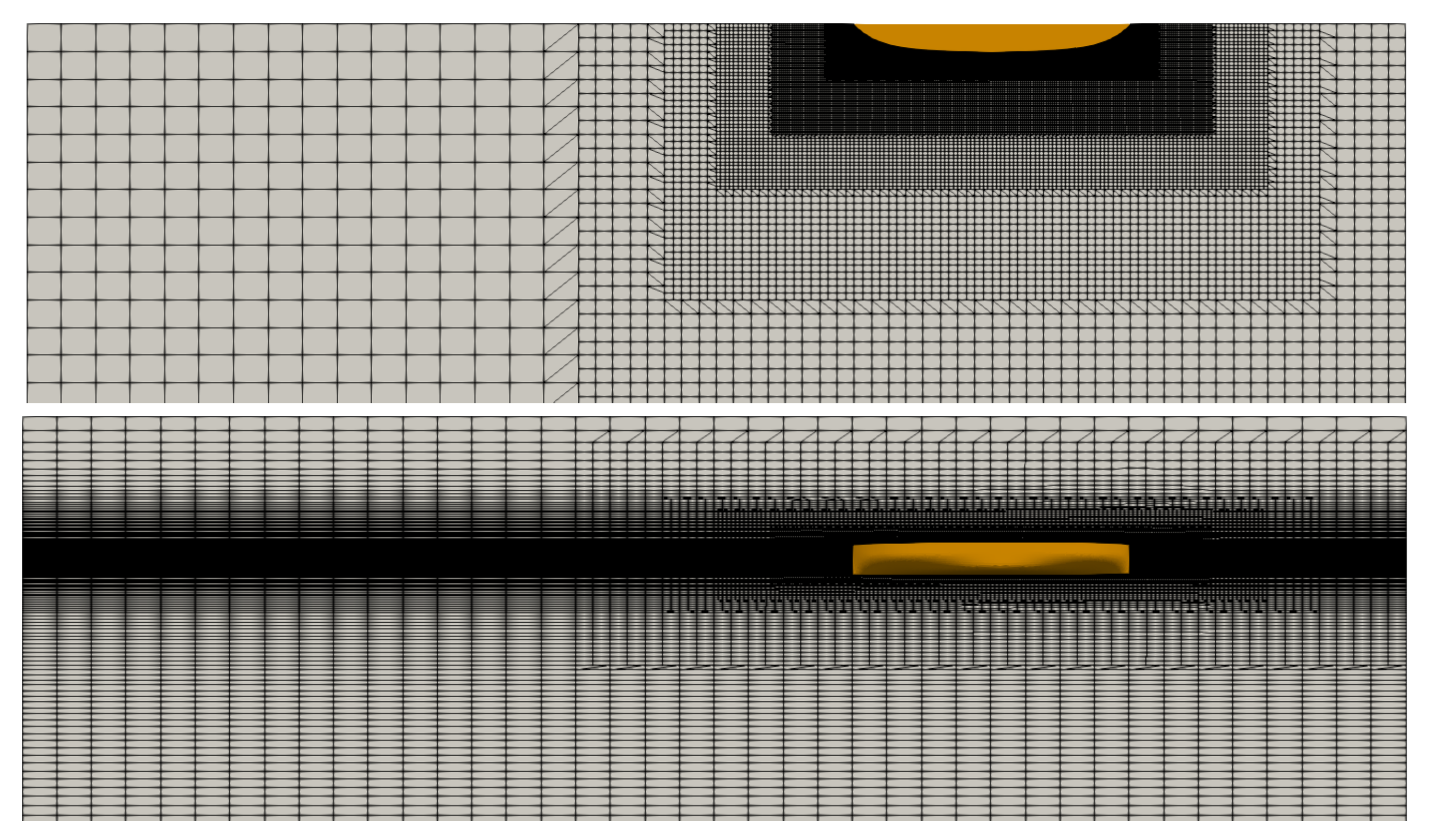
Unstructured mesh including hexahedral and tetrahedral cells was generated using snappyHexMesh tool of OpenFOAM. Top view and side view of the mesh in the computational domain are shown in Figure 3. Refinements with 5 different levels were used to refine the mesh around the hull and free surface. The finest mesh size was set to satisfy in the longitudinal direction and in the vertical direction. In addition, five layers of thin cells were added for the boundary layer around the ship hull. The first layer of cells around the ship hull was set to satisfy the nondimensional thickness of the cell , where (U is the ship speed, denotes the thickness of the first layer of cell, represents kinematic viscosity of the fluid). Meanwhile, standard wall functions were applied to computing at the first off-wall nodes ( represents turbulence kinematic viscosity).
4. Results and Discussions
4.1. Code Validation
To carry out a validation for the wave model, the same wave parameters to Kashiwagi (2013) [29] were used (see Table 2). Seven cases with different wave lengths were then implemented for model 1. The nondimensional total resistance of the hull was defined as
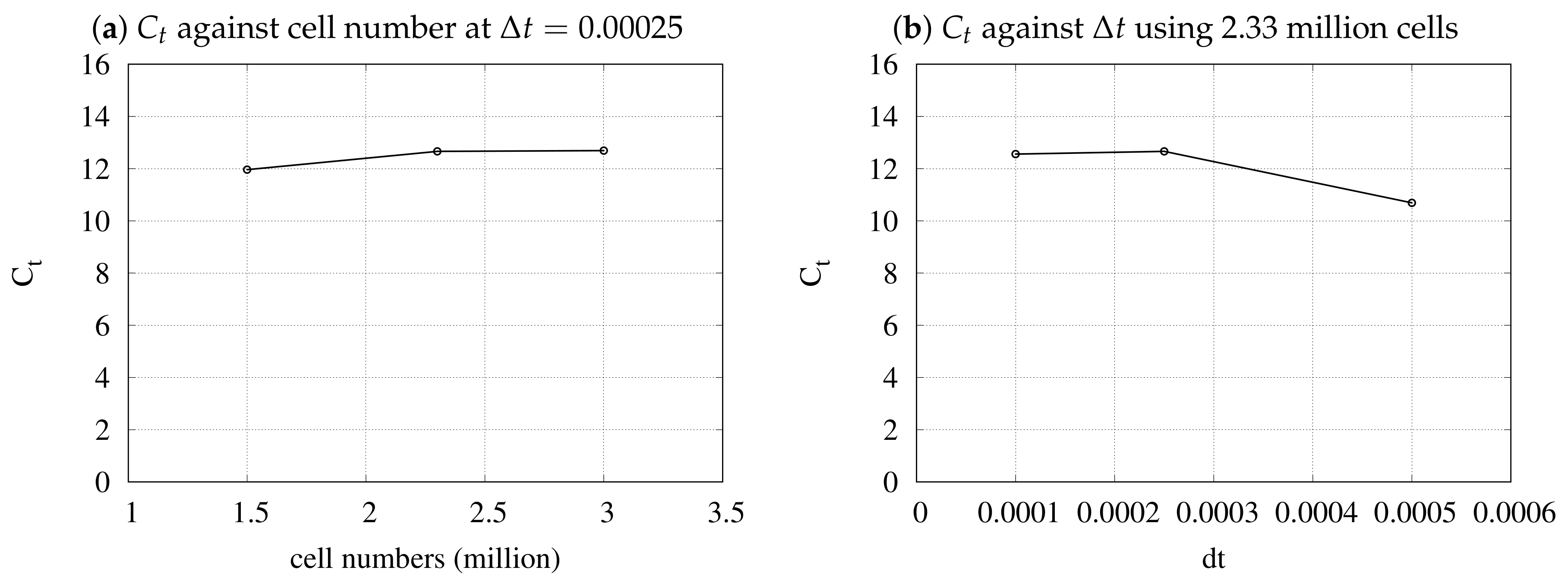
and was computed using 1.51, 2.33 and 3.02 million cells of meshes and three time steps () to test the grid and time step convergence (see Figure 4). In Equation (23) denotes the mean resistance of the hull in waves. The figure shows the convergence and a mesh with about 2.33 million cells and was adopted for all the further simulations.
In the simulation of each case, 15 encounter periods () of computation, which takes about 50 CPU hours of high performance computing with eight Intel Xeon Gold processors, were undertaken and 10 periods of data were used to calculate the results of the wave-induced motion and resistance after the system reached a steadily periodic state. Time histories of heave and pitch were expanded into Fourier series
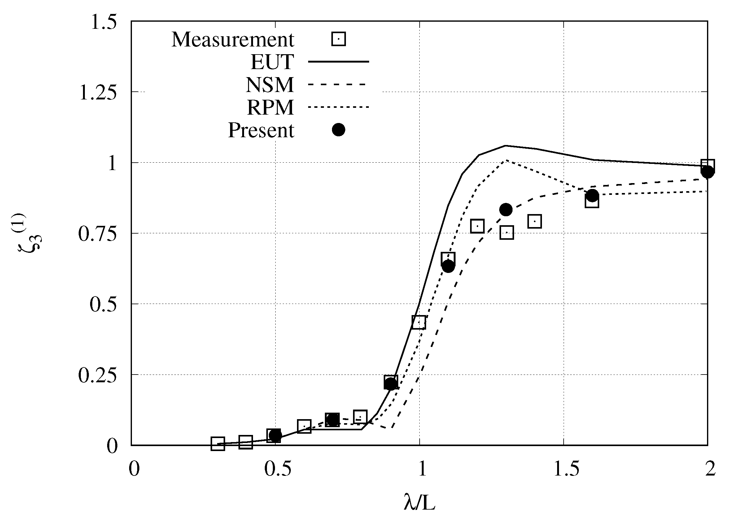
where is the nth harmonic amplitude and is the corresponding phase angle. The nth dimensionless harmonic amplitudes of the heave () and pitch () were then obtained using Fourier transformation. Profiles of the first harmonic amplitude of heave over a range of dimensionless wave length () are shown in Figure 5. Experimental data, computed results by Enhanced Unified Theory (EUT), New Strip Method (NSM) and Rankine Panel Method (RPM) originally introduced by Kashiwagi (1995 [33], 2013 [29]), Iwashita and Ito (1998) [34] are also included in this comparison. Both EUT and RPM are frequency-domain linear calculation methods, in which the disturbed flow is divided into the steady () and unsteady () flows. In EUT, the steady disturbance potential is ignored. In RPM it is computed numerically as double-body flow and its effects on the body and free-surface boundary conditions are considered. In NSM hydrodynamic actions on and motions of the ship are determined by integrating the results from two-dimensional hydrodynamic coefficients over the ship length. As shown in Figure 5, EUT and NSM are not in good agreement with the experimental results. In general comparisons against RPM are are good with the exception of .
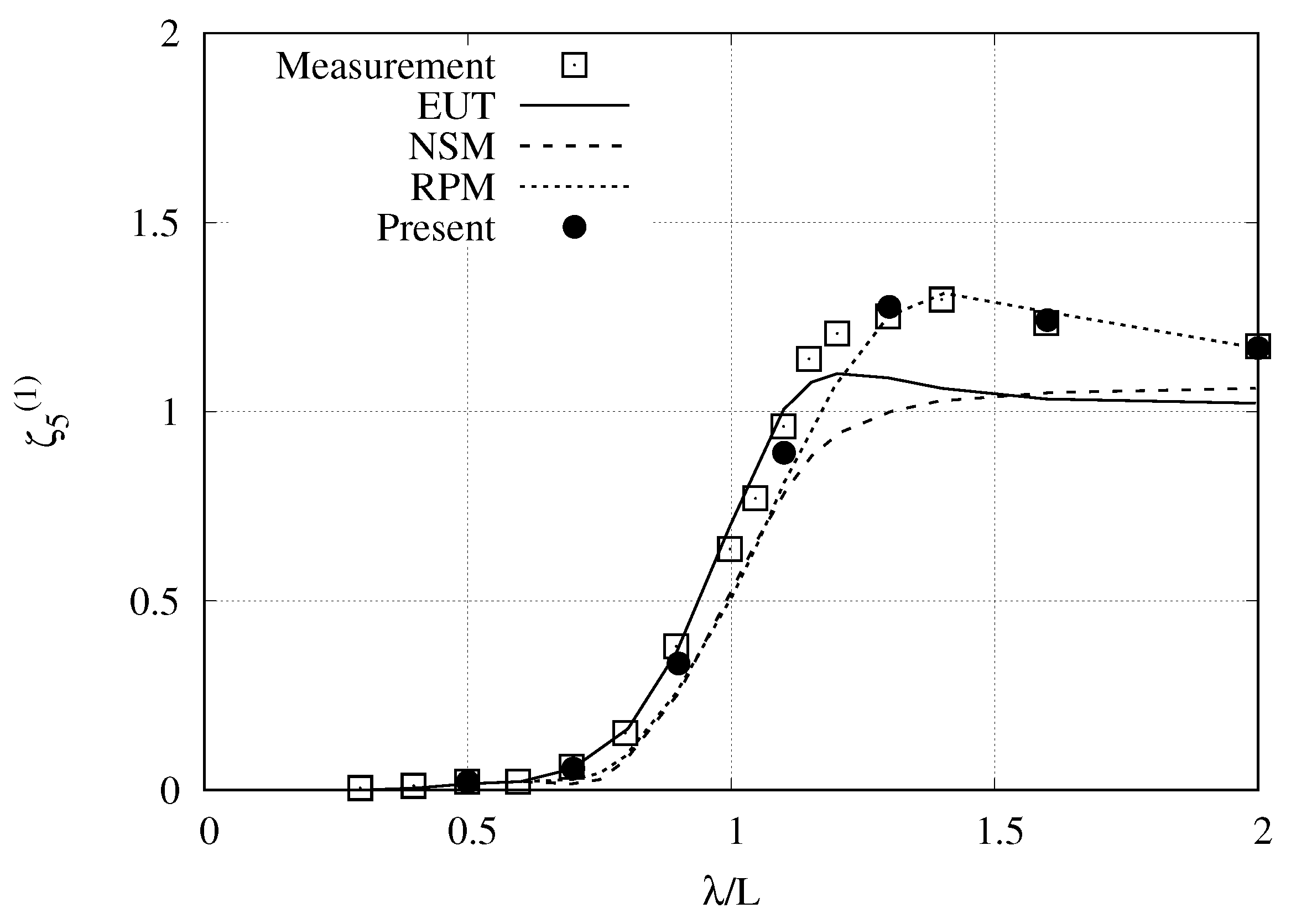
Variations of the first harmonic amplitude of pitch with the wave length are shown in Figure 6. Both EUT and NSM results do not coincide well with the experiments and visible underpredictions appear at large . Results obtained by the RPM model are less accurate than those obtained by the novel CFD method presented in this paper for .
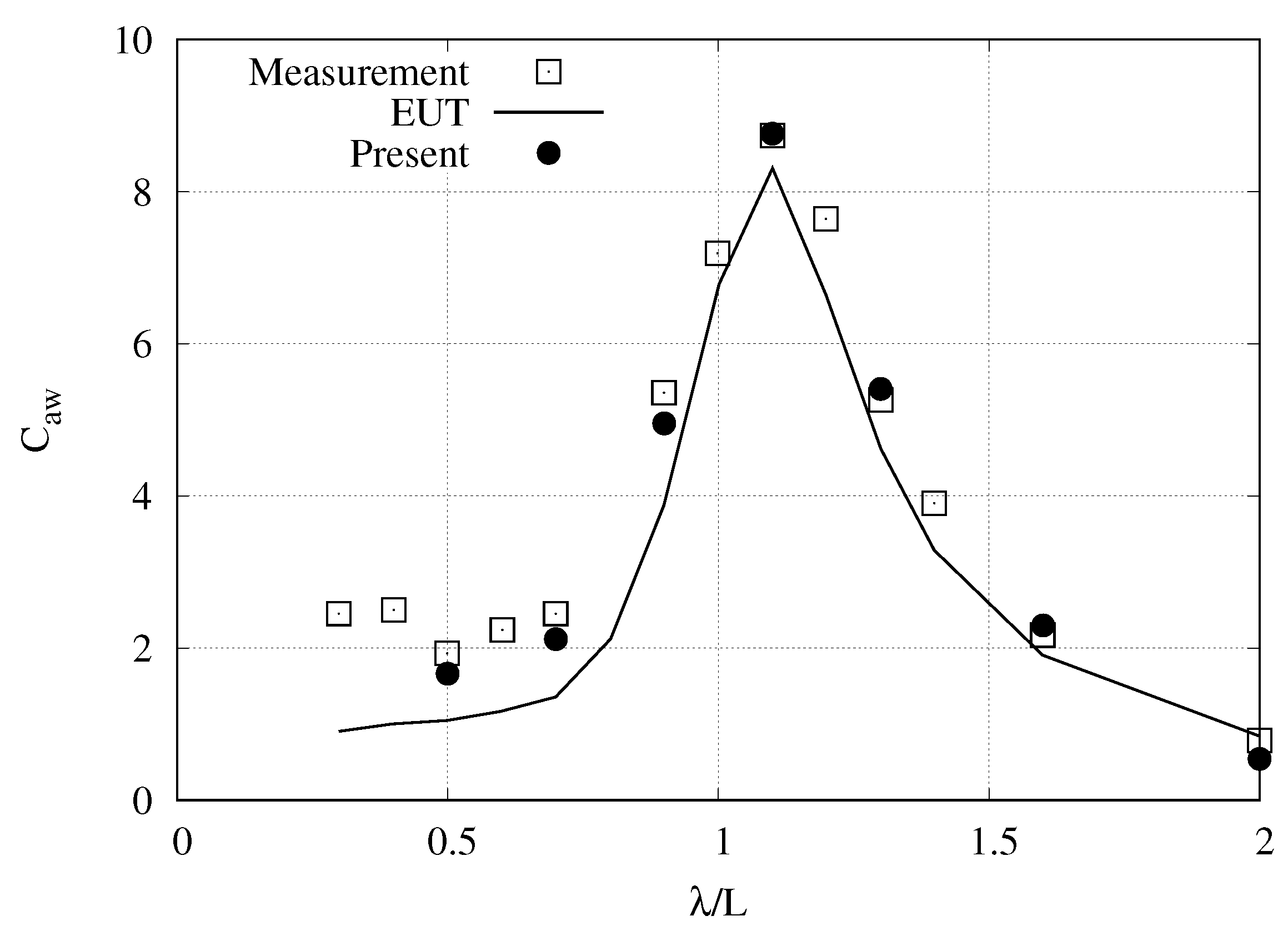
Added resistance is defined as a difference between the mean (time-averaged) resistance in waves and in calm water at the same speed U. The nondimensional added resistance was defined as
where and represent the mean resistance of the hull in waves and in calm water respectively; is the density of fluid; g is the gravitational acceleration; A is the wave amplitude; B and L are waterline breadth and length between perpendiculars of the ship respectively. Comparisons of the distributions of the nondimensional added resistance obtained by experiments, EUT and CFD are shown in Figure 7. It is shown that EUT underpredicts added resistance. CFD results are generally in better agreement with experiment. However, differences at low become more obvious.
4.2. Green Water on Decks
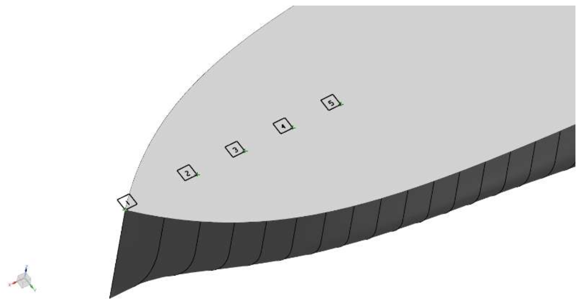
To observe the green water events, simulations associated with seven wave lengths were implemented in Model 2 (see Figure 1). The impact of green water on decks was examined by measuring the pressure at five monitoring points with coordinates (1.25, 0), (1.1, 0), (1.0, 0), (0.9, 0) and (0.8, 0) on the deck along the centreline of the bow (see Figure 8).
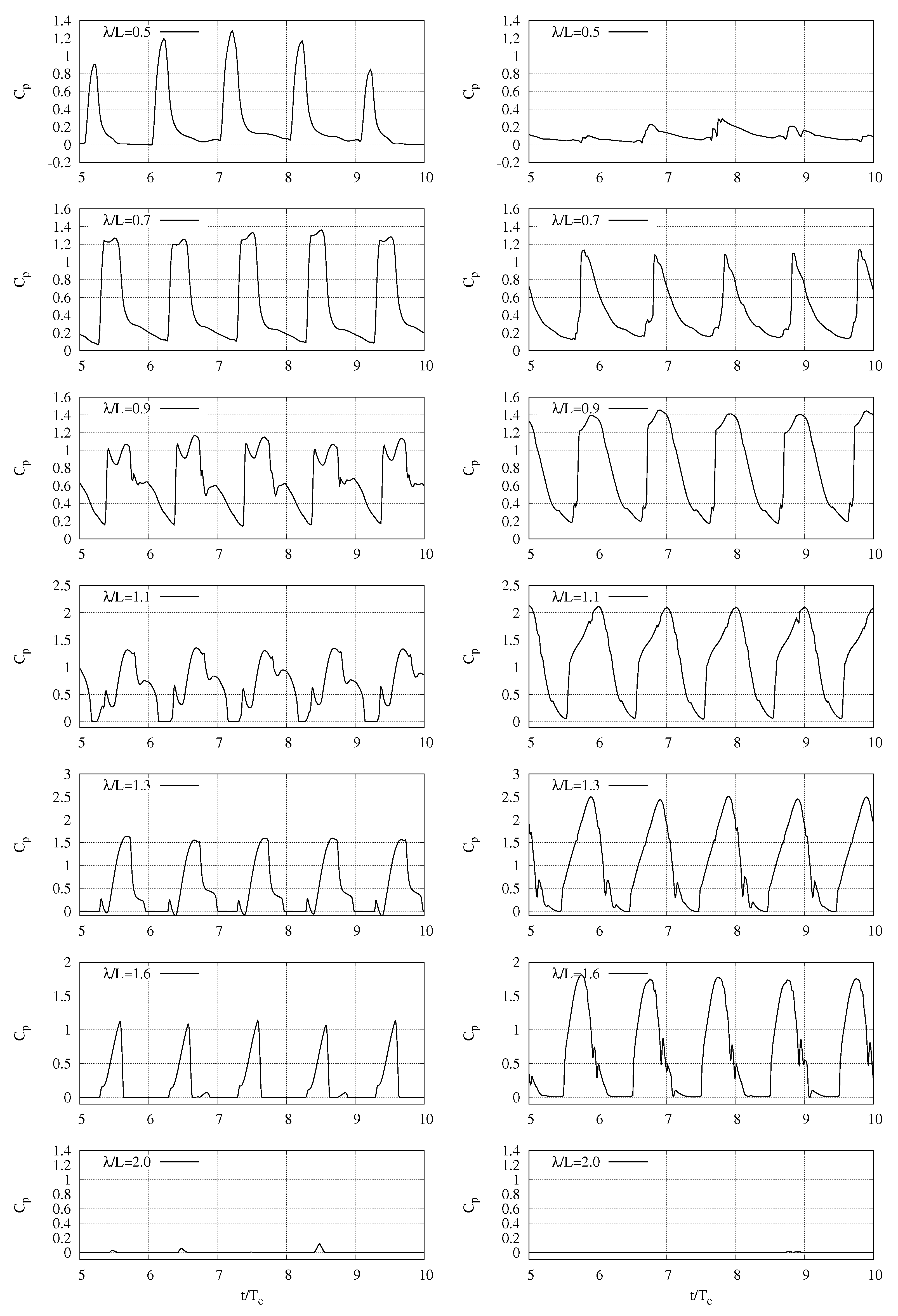
In green water events free surface exceeds the ship freeboard and hydrodynamic flow propagates over the deck with high-velocity. In way of impact the fluid flow pressure sharply increases. Figure 9 shows the variation of time histories of pressure coefficients over nondimensional time () in way of points 1 and 2 (see Figure 8). For each case the pressure coefficient was defined as
It was found that the green water impact at point 1 increased from to 0.7 and decreased from to 0.9. On the other hand, the pressure at point 2 is larger than that in way of point 1 at . This is because at green water becomes stronger and the water flow over the freeboard rapidly propagates downstream while an air layer is formed underneath. Eventually, an air bubble is entrapped inside the on-deck water. The pressure at point 2 increases from to 1.3 and reaches its highest value at . This implies that the highest influence of green water on decks occurs at . The green water event then starts to decline until it disappears at . Occurrence of the strongest green water impact is associated with the highest 1st harmonic amplitudes of the pitch.
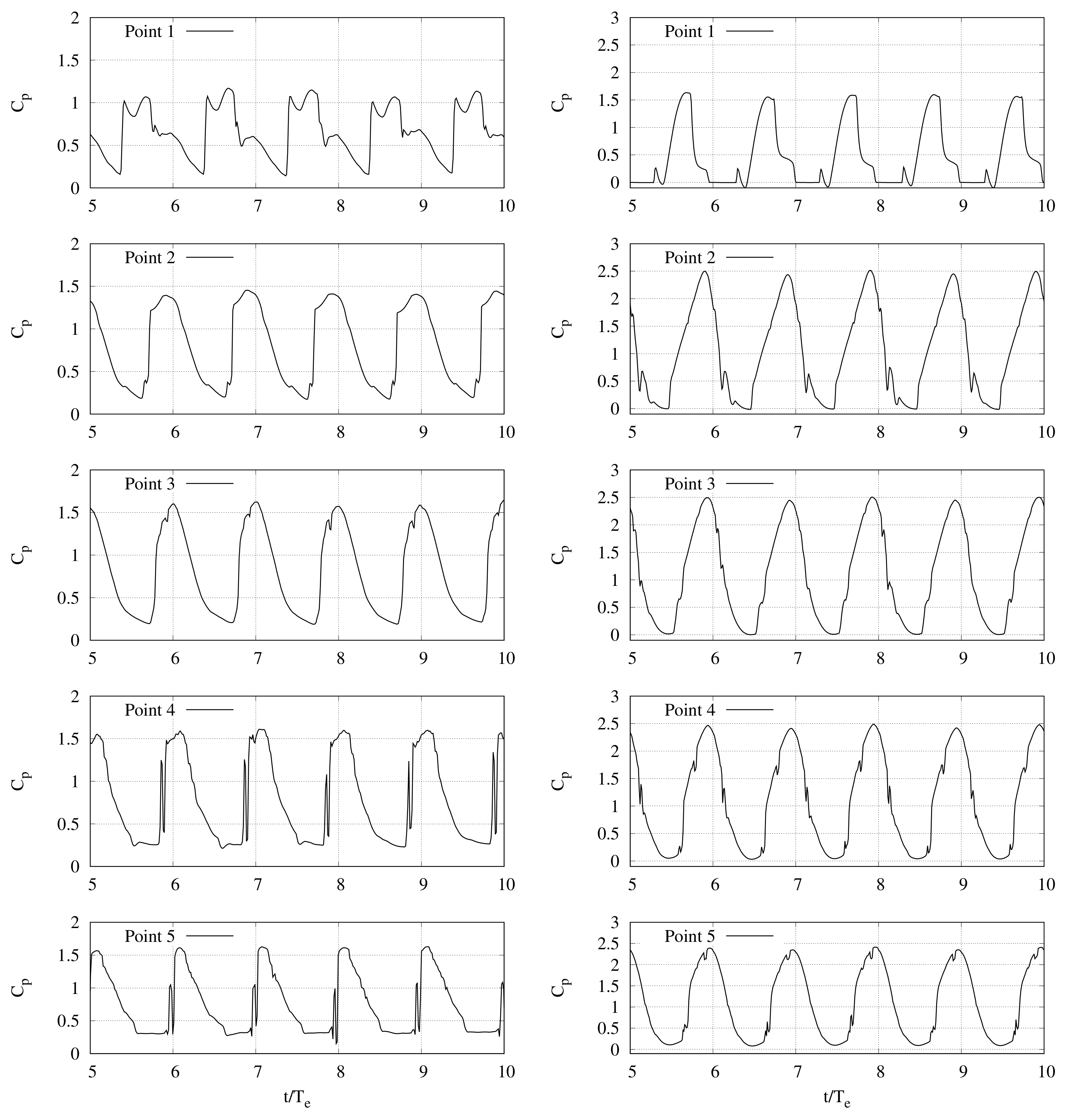
Figure 10 shows the pressure coefficient distributions over the time at five points for and 1.3. The profiles show that for pressures at all the monitoring points are smaller than those of . This confirms that the green water at is relatively weaker than at . This demonstrates that while a large amount of water exceeds the freeboard and keeps propagating along the deck, pressures remain high at the five monitored points. The time lag in pressure peaks experienced between point 1 and points 2 to 5 reflects that water first impacts point 1, then impacts point 2 as it climbs up the freeboard. The water rapidly spreads on deck (points 2–5) without major pressure fluctuations.
4.3. Flow Visualization
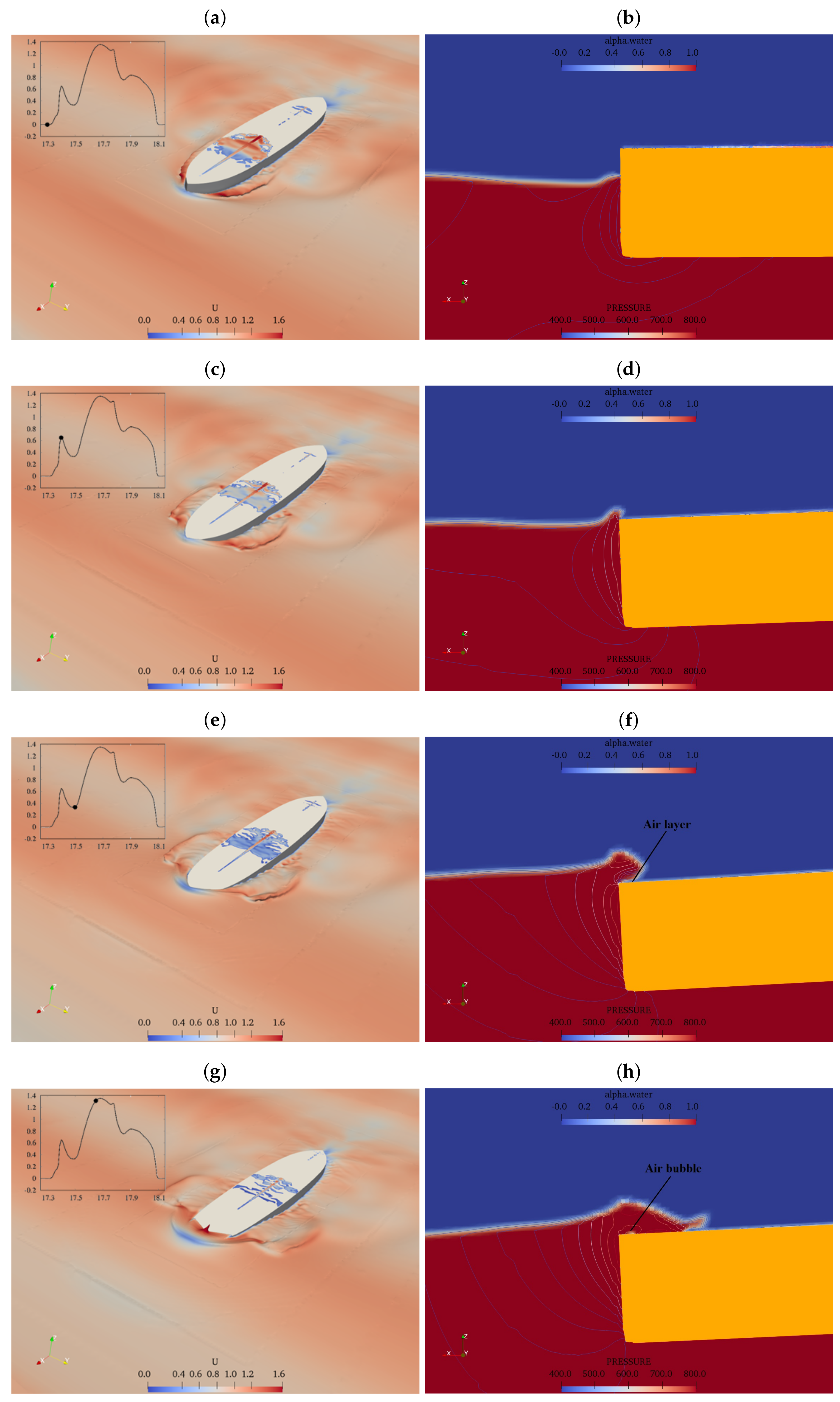
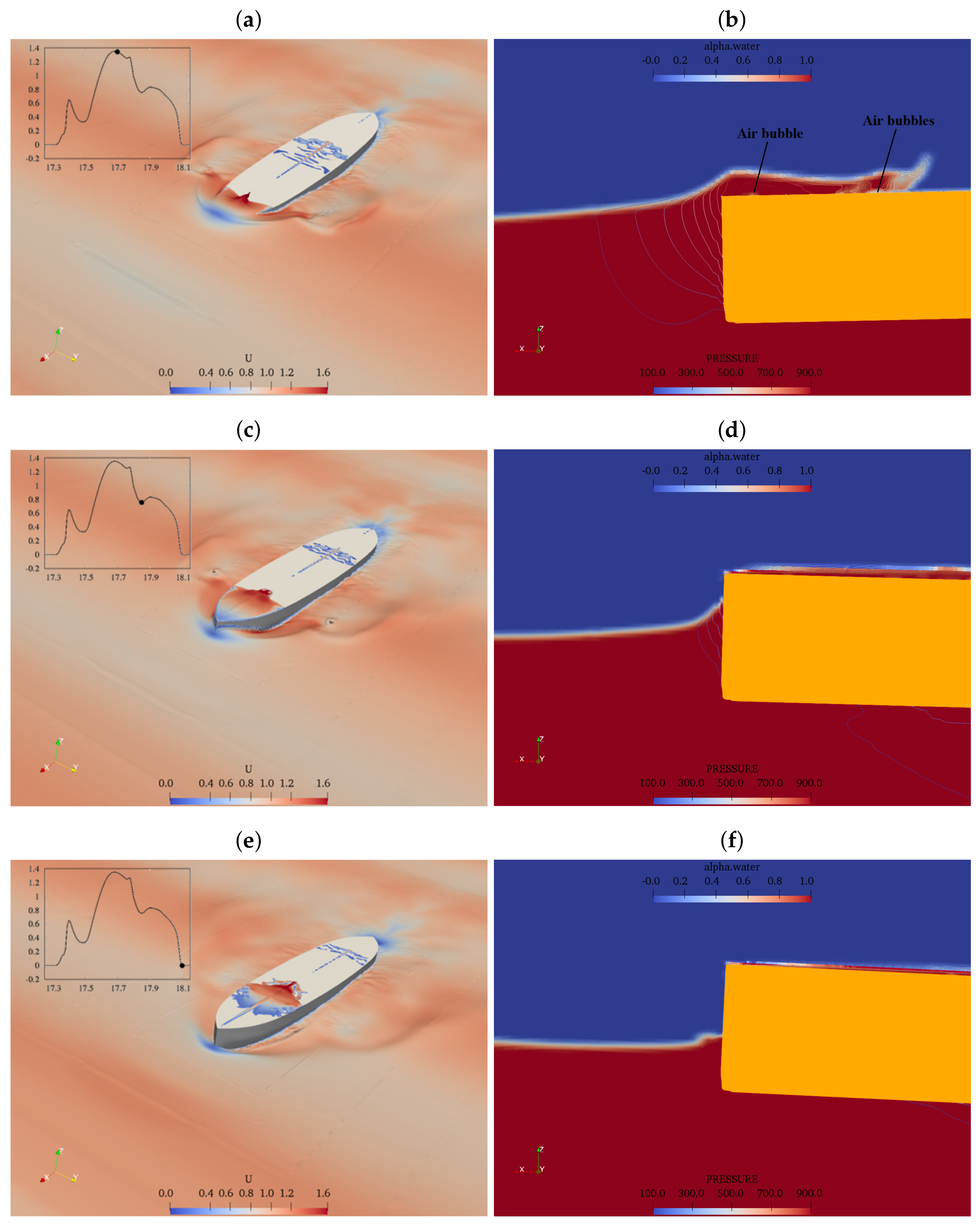
Flow visualization was achieved by plotting velocity contours on the free surface and pressure contours in way of the x-z plane at at seven instants in one motion period corresponding to . Free surface was defined at . As shown in Figure 11 and Figure 12 on the top left side of each flow velocity contour, the pressure profile at point 1 is attached to highlight the pressure magnitude. At first instance, the hull is almost at a horizontal state and the pressure at point 1 is low (see Figure 11a,b). At the second instant, a trim by the bow starts and wave-structure interaction causes climb up of the water above the bow height (see Figure 11c,d). Consequently, water impact with high-velocity flow causes sharp increase of pressure at point 1. At the third time instant, it can be seen that the pressure at point 1 decreases (see Figure 11e,f). This is because the water flow has very high velocity. As the vessel trims by the bow, a low pressure air layer grows between the water and the deck (see Figure 11f). At the fourth time instant, a trim by the aft starts and the wave-structure interaction becomes stronger (see Figure 11g,h). This causes the pressure at point 1 to reach its highest magnitude. When the trim by aft starts, the water over the deck rolls down and entraps the air underneath to form an air bubble in a form of a low-pressure zone on the deck bow (see Figure 11h). At the fifth time instant, the air bubble propagates downstream along the deck and air bubbles are formed downstream (see Figure 12a,b). At the sixth time instant, the hull trims by the aft, the bow is no longer submerged in waves and the on-deck water is starting to decline, thus leading to decrease of the pressure at point 1 (see Figure 12c,d). At the seventh instant, the volume of water at the deck bow continues to decline and some of on-deck water propagates downstream on the deck. This leads to lower pressure at the other four monitoring points (see Figure 12e,f). The free surface ahead of the bow is falling and the pressure at point 1 approaches its lowest magnitude.
4.4. Motion Quantities and Added Resistance
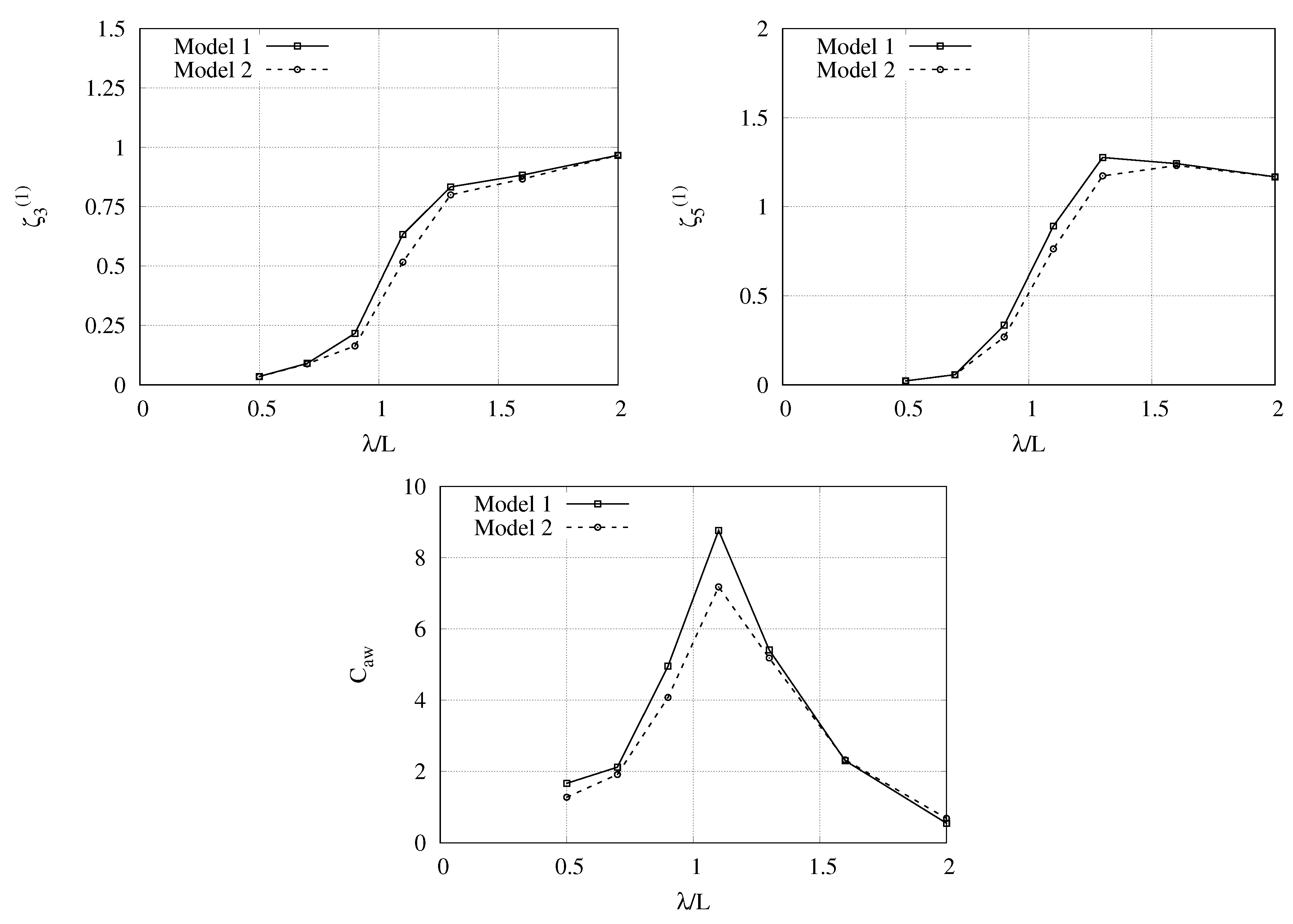
During the green water event, the wetted surface also decrease at the moment of occurrence of a trim by aft. This may lead to changes in the hydrodynamic forces on the hull. The green water impact would also have an effect on the hydrodynamic forces on the hull, variations in motions and added resistance. Figure 13 illustrates variations of heave, pitch and added resistance for both Wigley models (see Figure 1). It may be concluded that because of the higher free-board height of Model 2 in comparison to Model 1 the impact of green water on decks is low and does not influence that much the first harmonic heave/pitch amplitudes at , 0.7 and 1.6. For both models from to 1.3, the green water event remains strong, thus both the decrease of the wetted surface and the green water impact cause decreases of the first harmonic amplitudes of the heave and pitch as well as added resistance.
5. Conclusions
This paper presented 3D RANS CFD simulations for low and high freeboard Wigley hull models. Free surface effects were solved by the VOF method in the openFOAM numerical wave tank. Comparisons between computations and experimental results helped to validate fluid structure interaction modeling procedures, realise fluid flow phenomena and pressure peaks of relevance to the phenomenon of green water on decks. Results revealed that CFD simulations provide improved physics representation. The highest green water impact appears at at which the highest pitch is also present. For to 1.3, the water propagates far downstream and an air bubble is entrapped in a form of a small low-pressure zone.
Author Contributions
Conceptualization, L.C. and X.W.; methodology, L.C. and X.W.; validation, L.C. and X.C.; formal analysis, L.C. and X.C.; investigation, L.C.; writing–original draft preparation, L.C. and Y.W.; writing–review and editing, L.C., Y.W. and X.W.; visualization, L.C., Y.W. and X.C.; supervision, X.W.; project administration, L.C.; funding acquisition, L.C. All authors have read and agreed to the published version of the manuscript.
Funding
This research was funded by the Natural Science Foundation of Jiangsu Province (grant no. SBK2018040999) and Major Basic Research Project of the Natural Science Foundation of the Jiangsu Higher Education Institutions (18KJB570001).
Conflicts of Interest
The authors declare no conflict of interest.
References
- He, G.; Zhang, Z.; Tian, N.; Wang, Z. Nonlinear analysis of green water impact on forward-speed Wigley hull. In Proceedings of the 27th International Offshore and Polar Engineering Conference, San Francisco, CA, USA, 25–30 June 2017. [Google Scholar]
- Chen, L.; Taylor, P.H.; Draper, S.; Wolgamot, H. 3-D numerical modelling of greenwater loading on fixed ship-shaped FPSOs. J. Fluids Struct. 2019, 84, 283–301. [Google Scholar] [CrossRef]
- Buchner, B. Green Water on Ship-Type Offshore Structures. Ph.D. Thesis, Delft University of Technology, Delft, The Netherlands, 2002. [Google Scholar]
- Schiller, R.; Pakozdi, C.; Stansberg, C.; Yuba, D.; Carvalho, D. Green water on FPSO predicted by a practical engineering method and validated agianst model test data for irregular waves. In Proceedings of the ASME International Conference on Ocean, Offshore and Arctic Engineering—OMAE, San Francisco, CA, USA, 8–13 June 2014. [Google Scholar]
- Wang, S.; Wang, X.; Woo, W.L.; Seow, T.H. Study on green water prediction for FPSOs by a practical numerical approach. Ocean Eng. 2017, 143, 88–96. [Google Scholar] [CrossRef] [Green Version]
- Cox, D.T.; Scott, C.P. Exceedance probability for wave overtopping on a fixed deck. Ocean Eng. 2001, 28, 707–721. [Google Scholar] [CrossRef]
- Ogawa, Y.; Minami, M.; Tanizawa, K.; Kumano, A.; Matsunami, R.; Hayashi, T. Shipping water load due to deck wetness. In Proceedings of the Twelfth International Offshore and Polar Engineering Conference, Kitakyushu, Japan, 26–31 May 2002. [Google Scholar]
- Soares, C.G.; Fonseca, N.; Pascoal, R. Experimental and numerical study of the motions of a turret moored FPSO in waves. J. Offshore Mech. Arct. Eng. 2004, 127, 197–204. [Google Scholar] [CrossRef]
- Werter, R. Green Water Along the Side of an FPSO. Ph.D. Thesis, Delft University of Technology, Delft, The Netherlands, 2016. [Google Scholar]
- Buchner, B. The impact of green water on FPSO design. In Proceedings of the 27th Offshore Technology Conference, Houston, TX, USA, 1–4 May 1995. [Google Scholar]
- Schonberg, T.; Rainey, R.C.T. A hydrodynamic model of green water incidents. Appl. Ocean Res. 2002, 24, 299–307. [Google Scholar] [CrossRef]
- Yilmaz, O.; Incecik, A.; Han, J. Simulation of green water flow on deck using non-linear dam breaking theory. Ocean Eng. 2003, 30, 601–610. [Google Scholar] [CrossRef]
- Ryu, Y.; Chang, K.A.; Mercier, R. Application of dam-break flow to green water prediction. Appl. Ocean Res. 2007, 29, 128–136. [Google Scholar] [CrossRef]
- Pakozdi, C.; de Carvalho e Silva, D.; Ostman, A.; Stansberg, C. Green water on FPSO analyzed by a coupled potential-flow-NS-VOF method. In Proceedings of the International Conference on Offshore Mechanics and Arctic Engineering—OMAE, San Francisco, CA, USA, 8–13 June 2014. [Google Scholar]
- Zhou, Z.; Kat, J.; Buchner, B. A nonlinear 3-D approach to simulate green water dynamics on deck. In Proceedings of the Seventh International Conference on Numerical Ship Hydrodynamics, Nantes, France, 19–22 July 1999. [Google Scholar]
- Greco, M.; Lugni, C. 3-D seakeeping analysis with water on deck and slamming. Part 1: Numerical solver. J. Fluids Struct. 2012, 33, 127–147. [Google Scholar] [CrossRef]
- Zhang, S.; Yue, D.K.P.; Tanizawa, K. Simulation of plunging wave impact on a vertical wall. J. Fluid Mech. 1996, 327, 221–254. [Google Scholar] [CrossRef]
- Greco, M. A Two-Dimensional Study of Green-Water Loading. Ph.D. Thesis, Norwegian University of Science and Technology, Trondheim, Norway, 2001. [Google Scholar]
- Pham, X.P.; Varyani, K.S. Evaluation of green water loads on high-speed containership using CFD. Ocean Eng. 2005, 32, 571–585. [Google Scholar] [CrossRef]
- Greco, M.; Colicchio, G.; Faltinsen, O.M. Shipping of water on a two-dimensional structure. Part 2. J. Fluid Mech. 2007, 581, 371–399. [Google Scholar] [CrossRef]
- Shen, Z.; Wan, D. RANS computations of added resistance and motions of a ship in head waves. Int. J. Offshore Polar Eng. 2013, 23, 263–271. [Google Scholar]
- Nielsen, K.B.; Mayer, S. Numerical prediction of green water incidents. Ocean Eng. 2004, 31, 363–399. [Google Scholar] [CrossRef]
- Lu, H.; Yang, C.; L?hner, R. Numerical studies of green water impact on fixed and moving bodies. Int. J. Offshore Polar Eng. 2012, 22, 123–132. [Google Scholar]
- Zhao, X.; Hu, C. Numerical and experimental study on a 2-D floating body under extreme wave conditions. Appl. Ocean Res. 2012, 35, 1–13. [Google Scholar] [CrossRef]
- Zha, R.; YE, H.; Shen, Z.; Wan, D. Numerical computations of resistance of high speed catamaran in calm water. J. Hydrodyn. 2014, 26, 930–938. [Google Scholar] [CrossRef]
- Ostman, A.; Sileo, C.; Stansberg, C.; Fonseca de Carvalho e Silva, D. A fully nonlinear RANS-VOF numerical wave tank applied in the analysis of green water on FPSO in waves. In Proceedings of the International Conference on Offshore Mechanics and Arctic Engineering—OMAE, San Francisco, CA, USA, 8–13 June 2014. [Google Scholar]
- Kim, M.; Hizir, O.; Turan, O.; Incecik, A. Numerical studies on added resistance and motions of KVLCC2 in head seas for various ship speeds. Ocean Eng. 2017, 140, 466–476. [Google Scholar] [CrossRef] [Green Version]
- Chen, S.; Hino, T.; Ma, N.; Gu, X. RANS investigation of influence of wave steepness on ship motions and added resistance in regular waves. J. Mar. Sci. Technol. 2018, 23, 991–1003. [Google Scholar] [CrossRef] [Green Version]
- Kashiwagi, M. Hydrodynamic study on added resistance using unsteady wave analysis. J. Mar. Sci. Technol. 2018, 23, 991–1003. [Google Scholar] [CrossRef]
- Menter, F.R. Two-equation eddy-viscosity turbulence models for engineering applications. AIAA J. 1994, 32, 1598–1605. [Google Scholar] [CrossRef] [Green Version]
- Hirt, C.; Nichols, B. Volume of fluid (VOF) method for the dynamics of free boundaries. J. Comput. Phys. 1981, 39, 201–225. [Google Scholar] [CrossRef]
- Newmark, N.M. A Method of Computation for Structural Dynamics. J. Eng. Mech. Div. 1959, 85, 67–94. [Google Scholar]
- Kashiwagi, M. Prediction of surge and its effect on added resistance by means of the enhanced unified theory. Trans. West-Jpn. Soc. Naval Archit. 1995, 89, 77–89. [Google Scholar]
- Iwashita, H.; Ito, A. Seakeeping computations of a blunt ship capturing the influence of the steady flow. J. Ship Technol. Res. 1998, 45, 159–171. [Google Scholar]
Figure 1.
Forward views of the blunt Wigley hull models.

Figure 2.
Top view of the layout () of the computational domain with , , . The direction of x axis is opposite to the incoming flow, y axis is parallel to the free surface, the direction of z axis is opposite to the gravity.
Figure 2.
Top view of the layout () of the computational domain with , , . The direction of x axis is opposite to the incoming flow, y axis is parallel to the free surface, the direction of z axis is opposite to the gravity.

Figure 3.
Top and side view of the mesh for the computational domain. Upper one: top view; lower one: side view.
Figure 3.
Top and side view of the mesh for the computational domain. Upper one: top view; lower one: side view.

Figure 4.
Total resistance computation of model 1 at for testing grid and time step convergence.

Figure 5.
The first harmonic amplitude of the heave against the wave length.

Figure 6.
The first harmonic amplitude of the pitch against the wave length.

Figure 7.
Added resistance of model 1 versus .

Figure 8.
Monitoring points (Point 1 to 5 starting from the bow) on the deck for the pressure measurement.
Figure 8.
Monitoring points (Point 1 to 5 starting from the bow) on the deck for the pressure measurement.

Figure 9.
Time histories of the pressure coefficients at point 1 (left column) and point 2 (right column).
Figure 9.
Time histories of the pressure coefficients at point 1 (left column) and point 2 (right column).

Figure 10.
Time histories of the pressure at five monitoring points for (left column) and 1.3 (right column).
Figure 10.
Time histories of the pressure at five monitoring points for (left column) and 1.3 (right column).

Figure 11.
Flow velocity contours on the free surface (a,c,e,g) and pressure contours on the x–z plane at y = 0 (b,d,f,h) at time instants 1–4 for λ/L = 1.1.
Figure 11.
Flow velocity contours on the free surface (a,c,e,g) and pressure contours on the x–z plane at y = 0 (b,d,f,h) at time instants 1–4 for λ/L = 1.1.

Figure 12.
Flow velocity contours on the free surface (a,c,e) and pressure contours on the x–z plane at y = 0 (b,d,f) at time instants 5–7 for λ/L = 1.1.
Figure 12.
Flow velocity contours on the free surface (a,c,e) and pressure contours on the x–z plane at y = 0 (b,d,f) at time instants 5–7 for λ/L = 1.1.

Figure 13.
Profiles of heave, pitch and added resistance of the two models against .


Table 1.
Principle parameters of the ship model.
| Length between perpendiculars, L (m) | 2.5 |
| Waterline breadth, (m) | 0.5 |
| Draft, (m) | 0.175 |
| Displacement volume, V (m) | 0.139 |
| Height of gravity center, (m) | 0.145 |
| Gyration radius in pitch, | 0.236 |
| Freeboard height, f (m) | 0.175 (model 1), 0.0875 (model 2) |
Table 2.
Wave parameters for the simulations.
| Froude Number, | Wave Amplitude, | Wave Length, | Wave Steepness, | Encounter Frequency, |
|---|---|---|---|---|
| 0.5 | 0.048 | 11.998 | ||
| 0.7 | 0.0343 | 9.49 | ||
| 0.9 | 0.02667 | 7.996 | ||
| 0.2 | 0.012 | 1.1 | 0.0218 | 6.994 |
| 1.3 | 0.01846 | 6.267 | ||
| 1.6 | 0.015 | 5.48 | ||
| 2.0 | 0.012 | 4.75 |
© 2020 by the authors. Licensee MDPI, Basel, Switzerland. This article is an open access article distributed under the terms and conditions of the Creative Commons Attribution (CC BY) license (http://creativecommons.org/licenses/by/4.0/).
Share and Cite
MDPI and ACS Style
Chen, L.; Wang, Y.; Wang, X.; Cao, X. 3D Numerical Simulations of Green Water Impact on Forward-Speed Wigley Hull Using Open Source Codes. J. Mar. Sci. Eng. 2020, 8, 327. https://doi.org/10.3390/jmse8050327
AMA Style
Chen L, Wang Y, Wang X, Cao X. 3D Numerical Simulations of Green Water Impact on Forward-Speed Wigley Hull Using Open Source Codes. Journal of Marine Science and Engineering. 2020; 8(5):327. https://doi.org/10.3390/jmse8050327
Chicago/Turabian StyleChen, Linfeng, Yitao Wang, Xueliang Wang, and Xueshen Cao. 2020. "3D Numerical Simulations of Green Water Impact on Forward-Speed Wigley Hull Using Open Source Codes" Journal of Marine Science and Engineering 8, no. 5: 327. https://doi.org/10.3390/jmse8050327
Note that from the first issue of 2016, this journal uses article numbers instead of page numbers. See further details here.