Experimental Validation of Single- and Two-Phase Smoothed Particle Hydrodynamics on Sloshing in a Prismatic Tank

1
Graduate School of Maritime Sciences, Kobe University, Kobe 658-0022, Japan
2
Department of Naval Architecture, Diponegoro University, Semarang 50275, Indonesia
3
Kobe Ocean-Bottom Exploration Center, Kobe University, Kobe 658-0022, Japan
4
National Research Institute of Fisheries Engineering, Japan Fisheries Research and Education Agency, Kamisu 314-0408, Japan
*
Author to whom correspondence should be addressed.
J. Mar. Sci. Eng. 2019, 7(8), 247; https://doi.org/10.3390/jmse7080247
Submission received: 31 May 2019
/
Revised: 10 July 2019
/
Accepted: 25 July 2019
/
Published: 28 July 2019
(This article belongs to the Section Ocean Engineering)
Abstract
:This study aimed to validate the single-phase and two-phase smoothed particle hydrodynamics (SPH) on sloshing in a tank. There have been many studies on sloshing in tanks based on meshless particle methods, but few researchers have used a large number of particles because there is a limitation on the total number of particles when using only CPUs. Additionally, few studies have investigated the influence of air phase on tank sloshing based on two-phase SPH. In this study, a dedicated sloshing experiment was conducted at the National Research Institute of Fishing Engineering using a prismatic tank with a four-degrees-of-freedom forced oscillation machine. Three pressure gauges were used to measure local pressure near the corners of the tank. The sloshing experiment was repeated for two different filling ratios, amplitudes, and frequencies of external oscillation. Next, a GPU-accelerated three-dimensional SPH simulation of sloshing was performed using the same conditions as the experiment with a large number of particles. Lastly, two-dimensional sloshing simulations based on single-phase and two-phase SPH were carried out to determine the importance of the air phase in terms of tank sloshing. Based on systematic comparisons of the single-phase SPH, two-phase SPH, and experimental results, this paper presents a detailed discussion of the role of air-phase in terms of sloshing. The currently achievable accuracy when using SPH is demonstrated together with a few sensitivity analyses of SPH parameters.
1. Introduction
The increasing demand for liquefied natural gas (LNG) has had a significant influence on the capacity of LNG carriers. During the marine transportation of LNG, there is a dangerous phenomenon called sloshing that can be defined as the resonance of fluid inside a tank caused by external oscillations (i.e., ship motion in the case of marine transportation). When a ship is subjected to external oscillation that is close to the natural frequency of the tanks it is carrying, severe sloshing can occur and cause damage to tanks based on the violent movement of fluid, which leads to a high impact pressure on tank walls. This high impact pressure can cause explosions when volatile fluids, such as oil, are transported on a ship. In recent decades, the demand for sloshing analysis has increased significantly in the shipping industry. Because sloshing is defined by nonlinear free surface flows, both physical experiments and numerical methods are commonly used for such an analysis.
Computational fluid dynamics (CFD) has been widely adopted as an advanced numerical approach. Mesh-based CFD is a standard method that numerically approximates a space using meshes. There have been several pioneering works on sloshing simulation using mesh-based CFD. Kishev et al. [1] developed a novel CFD simulation approach based on constraint interpolation profiles. Kim [2] investigated both 2D and 3D liquid sloshing in containers by using the synchronized overlap-and-add algorithm. Recently, the OpenFOAM software was used by Jiang et al. [3] to simulate sloshing coupled with ship motions. Sloshing with different filling levels was investigated experimentally by Chen and Xue [4].
Recently, particle methods, which are also known as mesh-free CFD, have been applied to tank sloshing problems. Because particle methods are fully Lagrangian and truly mesh-free approaches, mesh handling is not necessary and a significantly deformed free surface can be captured intuitively without any special treatment. Smoothed particle hydrodynamics (SPH) [5,6] is a popular particle method that was first extended for free surface flows by Monaghan [7]. Since then, there have been many applications of SPH to free surface flow problems. Dalrymple and Rogers [8] demonstrated that SPH is able to model breaking waves on a beach in both two and three dimensions. Makris et al. [9] used SPH to model wave breaking over a relatively mild slope in two dimensions. Antuono et al. [10] used delta-SPH for water waves and drew comparisons to a boundary element method mixed-Eulerian-Lagrangian solver. Altomare et al. [11] used SPH to model water waves and performed verification using the second-order Stokes theory. By using a general stabilizing algorithm based on Fick’s law, Lind et al. [12] simulated wave propagation accurately without decay. Colagrossi et al. [13] investigated the dissipation mechanisms of gravity waves and found that the number of neighboring particles is an important parameter for the convergence of results. Recently, an experimental validation of SPH for long-distance propagation was carried out by Trimulyono and Hashimoto using a large numerical wave tank [14]. The application of SPH to fluid-structure interactions was reported by Antoci et al. [15], who modeled the interactions between fluids and flexible gates based on 2D simulations. Crespo et al. [16], Altomare et al. [17], and Barreiro et al. [18] used SPH to predict impact forces on coastal structures. Wei et al. [19] as well as Sarfaraz and Park [20] performed SPH simulations to investigate the impact of tsunamis on bridge piers. Marrone et al. [21] presented SPH simulations for modelling viscous flows around blunt bodies at low and moderate Reynolds numbers. Zisis et al. [22] executed multiphase SPH simulations by applying a robust SPH number-density scheme and compared their method to the arbitrary Lagrangian Eulerian method. Kawamura et al. [23] reported the validation of SPH for ship motion in waves. Gómez-Gesteira et al. [24] performed SPH simulations to capture green water overtopping with a fixed horizontal deck. Le Touzé et al. [25] applied SPH to green water and ship flooding problems. Recently, a versatile algorithm for open boundaries in SPH was developed by Tafuni et al. [26] for 2D and 3D complex flows such as water waves and flows past a surface-piercing extraterrestrial submarine. Gonzalez-Cao et al. [27] made comparisons between SPH and the volume of fluid method to assess violent wave collisions on coastal structures. Verbrugghe et al. [28] used the open boundaries to perform water wave generation and absorption in one wavelength of wave flume and validation was carried out using a theoretical solution.
The application of SPH to sloshing problems has been carried out by Delorme et al. [29], Landrini et al. [30], and Chen et al. [31] to validate impact pressures based on SPH with forced roll motion in two dimensions. Kim [32] used SPH and the finite difference method to validate impact pressures using a rectangular tank. Colagrossi et al. [33] corrected pressure fields as a solution to pressure noise using an improved SPH method and Shao et al. [34] used kernel gradient correction and a novel treatment of solid boundaries to achieve a smoother distribution of the pressure field for a rectangular tank. Rafiee et al. [35] performed 2D and 3D SPH simulations of a rectangular tank under sway motion using an improved SPH method. Bouscasse et al. [36], and De Chowdhury and Sannasiraj [37] investigated shallow water sloshing using delta-SPH under sway motion with both small and large amplitudes of excitation. Recently, long-duration simulations of sloshing at small filling ratios were performed by Green and Peiro [38], who found that the SPH results matched experimental results in terms of both surface elevation and force on the tank. These results clearly demonstrate that SPH is suitable for evaluating the sloshing of nonlinear free surface flows. However, most past studies used simple rectangular tanks and single-phase SPH methods with relatively small numbers of particles. In this study, sloshing in a prismatic tank with sway and roll oscillations was investigated and experimental validation of both single-phase and two-phase SPH methods was attempted.
To perform large-scale SPH simulations, general-purpose computing on graphics processing units (GPGPU) technology can be advantageous because it facilitates the use of many compute unified device architecture (CUDA) cores on GPUs. In this study, a large-scale 3D sloshing simulation was carried out using an open-source SPH solver called DualSPHysics [39] that can be downloaded at https://dual.sphysics.org. DualSPHsysics is based on the SPHysics code and consists of a set of C++ and CUDA libraries for handling real-world engineering problems, such as sloshing and water waves. GPGPU has been implemented in DualSPHysics [40], but multiGPU computation has not yet been implemented. Computation decreases with the implementation of multiple GPUs, as shown by Dominquez et al. [41]. There are three main steps for SPH computation on a GPU: generation of a neighbor list, computation of the forces between particles, and updating of physical quantities prior to the next iteration. These steps are all executed on the GPU until the end of simulation. Some initial processing is performed on the CPU, then all data are transferred to GPU, where they continue to evolve in the GPU memory. Only a small amount of data are occasionally passed back to the host to be written to the disk [40]. All simulations in this study were performed using CUDA cores on a single GPU to handle a large number of particles and reduce computation time. In SPH simulations, the number of available particles is crucial not only for accuracy, but also for the application to realistic ocean engineering problems. GPGPU technology can realize efficient parallel computing for fully explicit time-marching schemes, such as SPH, which results in reliable and feasible solutions.
To validate the GPGPU SPH simulations of sloshing phenomena, a dedicated model experiment was conducted at the National Research Institute of Fishing Engineering (NRIFE). External sway and roll motions were generated for a prismatic tank by a four-degrees-of-freedom oscillation machine. The sloshing experiment was repeated for several different filling ratios, amplitudes, and frequencies of forced oscillation. The fluid behavior in the tank and the hydrodynamic pressures at different points were recorded. Next, 3D sloshing simulations based on single-phase SPH accelerated by a GPU with large numbers of particles were carried out and the results were compared to the experimental results. We found certain limits on single-phase SPH in terms of reproducible accuracy for the impact pressure. Next, 2D GPGPU simulations based on two-phase SPH were carried out to analyze the effects of the air phase on sloshing. Two-phase SPH simulations were carried out for two filling ratios with external sway and roll oscillations. By applying two-phase SPH to sloshing, the prediction accuracy for both global fluid behavior and local impact pressure can be improved. Through a systematic comparison study, validation of single-phase and two-phase SPH for sloshing phenomena is carried out and the importance of the air phase in sloshing problems is elucidated.
2. Numerical Methodology
SPH was initially developed for astrophysical problems and it has been widely used in marine engineering since its first application to a free-surface flow by Monaghan [7]. SPH is a fully Lagrangian meshless method that adopts an interpolation scheme to approximate the physical values and derivatives of a continuous field using discrete evaluation points. These evaluation points are identified as particles that contain mass, velocity, and position values. These quantities are obtained as weighted averages of adjacent particles within a smoothing length (h) to reduce the range of contributions from remote particles. The main features of the SPH method, which is based on integral interpolants, are described in detail in References [42,43]. In SPH, the field function A(r) in a domain Ω can be approximated using the integral approximation in Equation (1), where W is the kernel function and r is a position vector.
Equation (1) can be approximated in a discrete form by replacing the integral with a summation over neighboring particles in the compact support of particle a at the spatial position r. Therefore, the particle approximation of Equation (1) becomes the following.
where the volume associated with neighboring particle b is mb/ρb, where m, ρ denote mass and density, respectively. In discrete form, Equation (2) leads to an approximation of the function at particle a, as shown in Equation (3), where is a kernel function. Therefore, the derivative of these interpolants can be expressed by Equation (4).
The Lagrangian forms of the governing equations of the Navier-Stokes equation are
where D/Dt is the material derivative, ρ is density, P is pressure, is velocity, is gravitational acceleration, and represents diffusion terms. The capability of the SPH model depends on the choice of a kernel function. Kernel approximation is one of the main sources of errors in the SPH method. The selection of a kernel function not only affects computational efficiency, but also determines the accuracy and stability of the SPH method, as demonstrated by Cao et al. [44]. The kernel function must satisfy certain conditions, including the normalization condition, compact support, positivity, monotonic decrease with an increase in distance symmetric property, delta function property, and smoothness [43]. In this study, the Wendland kernel function [45] was used because it is computationally efficient and sufficiently smooth, as mentioned by Cao et al. [44]. This function is shown in Equation (8).
where is equal to (7/4) πh2 in 2D and (21/164) πh3 in 3D. q is the non-dimensional distance between particles a and b that is defined by r/h. The momentum equation to be solved in SPH is defined in Equation (9) for a water phase and Equation (10) for an air phase. The two-phase SPH method in DualSPHysics is based on a study by Colagrossi and Landrini [46], and it was developed by Mokos et al. [47].
where Pa and Pb are the pressures of particles a and b, respectively. is an artificial viscosity term defined by Monaghan [48], where . Additionally, , where r and v are position and velocity vectors, respectively, and is the mean speed of sound. Additionally, α is a coefficient that needs to be tuned to achieve proper dissipation.
The additional term in delta-SPH (), which was defined by Molteni and Colagrossi [49], is detailed in the paper by Antuono et al. [50,51]. This term was introduced to suppress density fluctuations. The equation of continuity with additional term of delta-SPH is defined in Equation (11).
DualSPHysics is based on weakly compressible smoothed particle hydrodynamics (WCSPH), where fluids are treated as weakly compressible. Therefore, the state equation defined in Equation (12) is used to determine the pressure field based on the computed particle density, where , c0 = c(ρ0) = , and γ = 7. c0, ρ0, and γ are the speed of sound at the reference density, the reference density itself, and the polytropic constant, respectively. In the two-phase SPH method, a modified state equation is introduced, as shown in Equation (13), where . ρw, ρa, L, and X are the initial water density, air density, characteristic length of the domain, and constant background pressure, respectively.
The time-stepping scheme used in this study is the second-order explicit symplectic defined by Leimkuhler et al. [52]. This is an integration algorithm that is accurate with a time complexity of O(). It utilizes the predictor and corrector stages defined below.
F consists of a pressure gradient term, diffusion term, and gravitational term, where the n-step indicates the time step and is the time increment of the n-step. Da is the divergence. The time step is calculated using the technique proposed by Monaghan et al. [53] as follows.
where is based on the force per unit mas () and Δtcv combines the Courant and viscous time step controls. CFL is a coefficient in the range of 0.1 ≤ CFL ≤ 0.3 [38]. Dynamic boundary particles (DBPs) are adopted based on the work by Crespo et al. [54]. DBPs are boundary particles that satisfy the same equations as fluid particles, but they do not move according to the forces exerted on them. Instead, they either remain fixed in position or move according to an imposed/assigned motion function (i.e., moving objects, such as gates, wavemakers, or floating objects). The particle shifting algorithm [12] was used to handle anisotropic particle spacing. When using the shifting algorithm, particles are moved to an area with fewer particles, which allows the domain to maintain a uniform particle distribution and eliminates voids to prevent noisy results.
3. Experimental Conditions
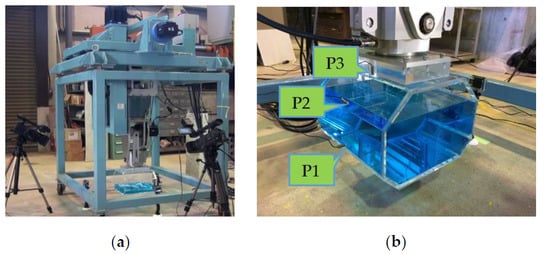
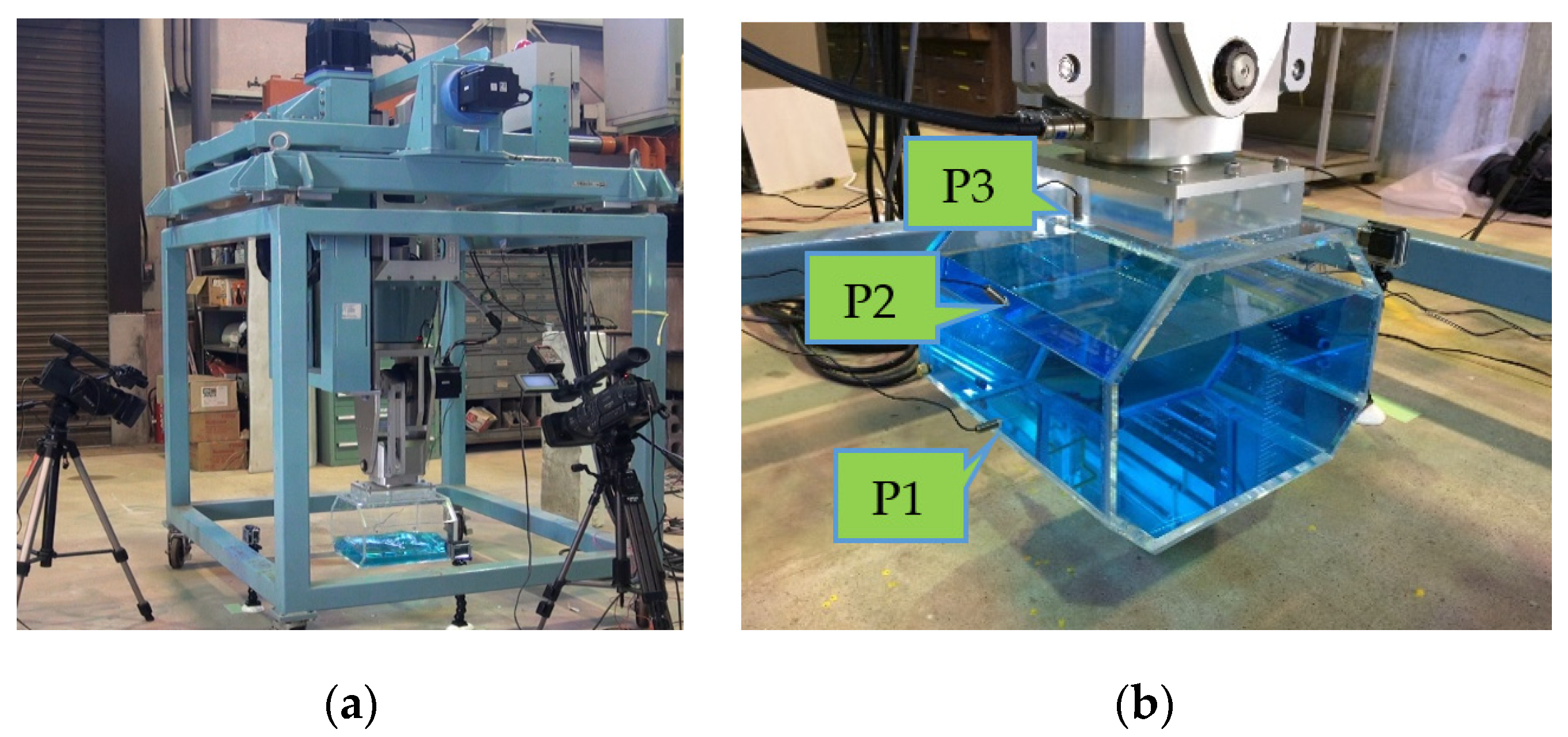
An experiment dedicated to the sloshing problem was recently conducted at the NRIFE using a prismatic tank. Figure 1a presents an overview of a sloshing test using a four-degree of freedom forced oscillation machine. Four video cameras were used in the sloshing test. Two were GoPro Hero cameras (GoPro Inc., San Mateo, CA, USA) that were placed near the tank to record the water behavior inside the tank and the other two cameras were used to record the external motion of the tank. Figure 1b presents the prismatic tank, which resembles a membrane-type LNG tank. The tank is scaled to 1:125 and the length is 0.36 m, the width is 0.30 m, and the height is 0.21 m. In the experiment, the tank was subjected to external sway, heave, roll, and yaw oscillations (see Table 1). Several amplitudes and frequencies were used for the forced oscillation test. The impact pressure caused by sloshing is an important factor because it can lead to structural damage. To measure the hydrodynamic pressure on the tank wall at different locations, pressure gauges (SSK Co., Ltd., Tokyo, JAPAN) were positioned at three locations (P1, P2, and P3), as shown in Figure 1b. P1 is near the bottom of the sidewall, and P2 and P3 are on the upper chamber. All gauges were positioned near corners to capture the impact pressure. Sloshing tests were conducted at filling ratios of 25% and 50%. The water height was 5.25 cm for the filling ratio of 25% and P1 was near the calm-water free surface. The water height was 10.5 cm for the filling ratio of 50%. A schematic view of the prismatic tank is presented in Figure 2. Table 2 lists the dimensions of the tank.
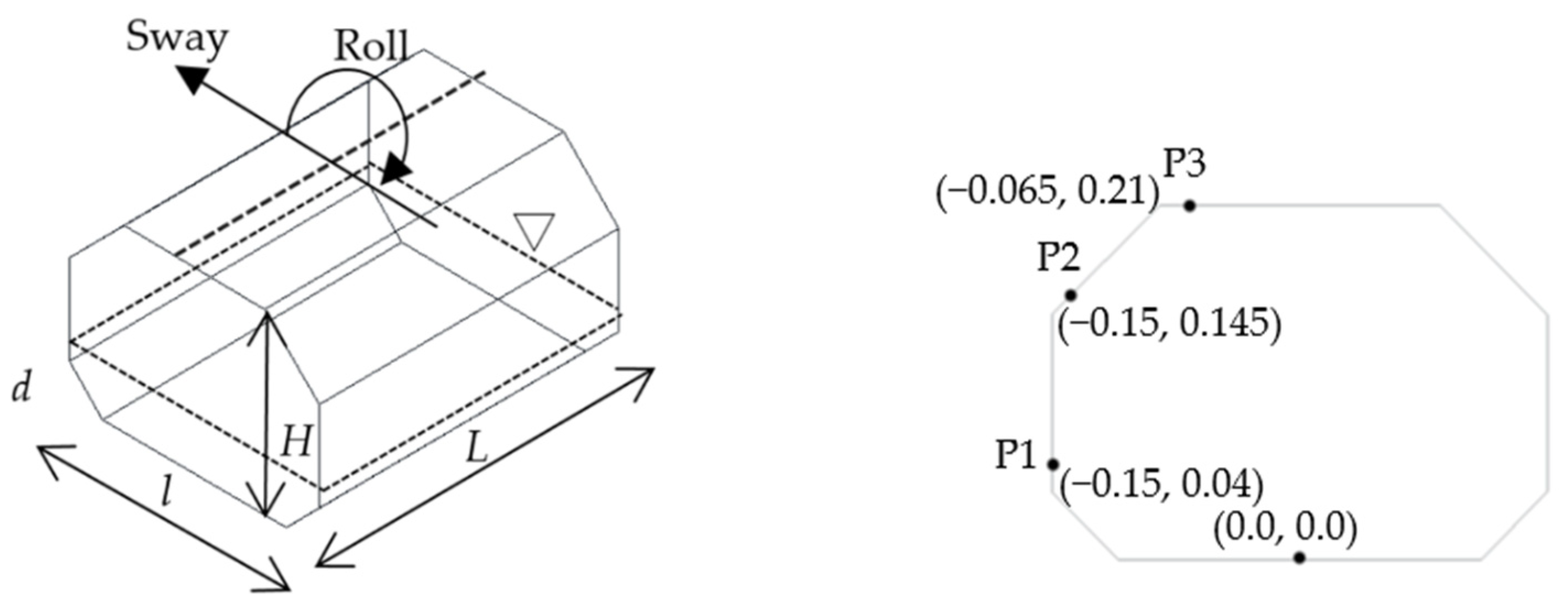
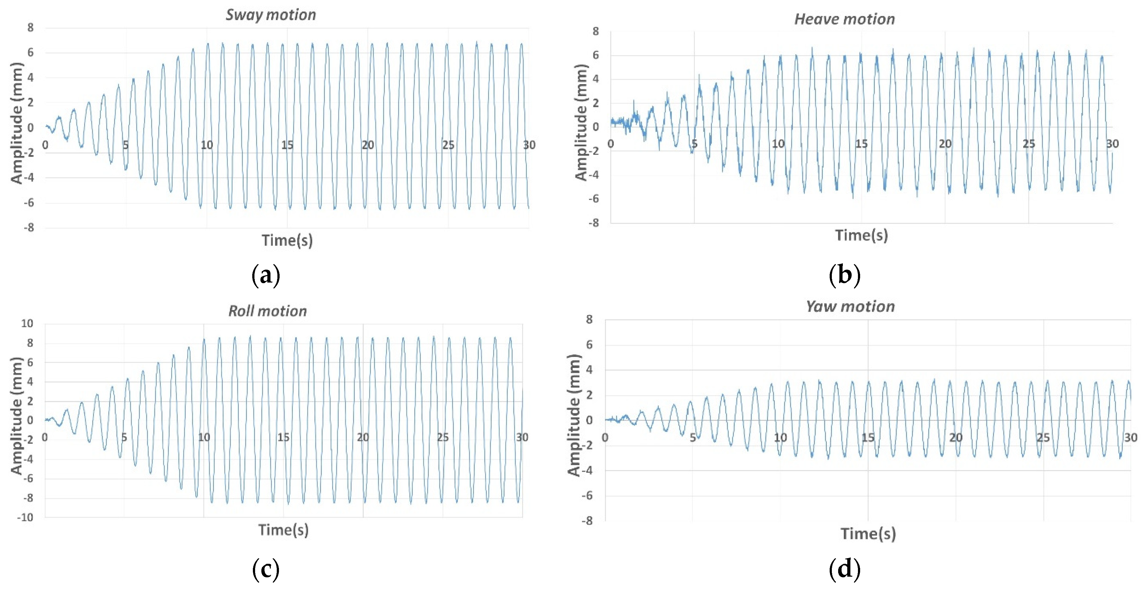
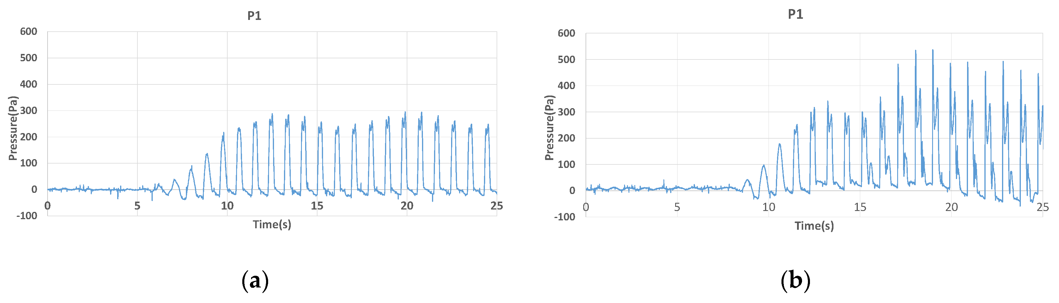
Figure 3 presents time histories of external oscillations with the maximum displacement imposed on the tank in each mode during the experiment. For all conditions, a simple linear ramping motion was applied for the first 10 seconds to avoid huge inertial forces. By directly imposing the measured displacements of the tank during SPH simulation, the SPH method can be validated in terms of fluid behavior, including complex free-surface evolution and the time history of local pressure (e.g., impact at the corners of the tank). In this paper, only the sway and roll motions are presented because sloshing cannot be observed when the tank is subjected to heave and yaw motions. Figure 4 presents the measured pressure at P1 with a filling ratio of 25%. In this paper, pressure refers to hydrodynamic pressure, which can be obtained by subtracting the analytical hydrostatic pressure under calm conditions from the measurement data. The sloshing caused by the roll motion is more violent when compared to that caused by the sway motion because the center of rotation is higher than the top of the tank for the roll motion.
The natural period of the prismatic tank was estimated using Equations (21) and (22), which were derived by Faltinsen and Timokha [55], where ωn is the natural frequency of the i-mode for a rectangular tank, d represents the water height, and l represents the length of the free surface in the direction of tank movement. For a prismatic tank with a chamfered bottom, a correction factor was introduced in Equation (22), where δ1 and δ2 are the horizontal and vertical dimensions of the chamfer, respectively.
4. Numerical Setup
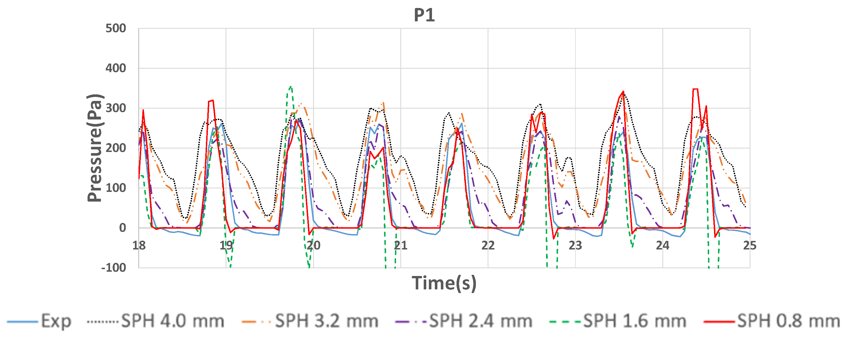
A tank with the same dimensions as that used in the experiment was used for SPH simulation to reproduce the sloshing phenomena observed in the experiment. A filling ratio of 25% was selected and the pressure gauge at P1 was located near the water surface. External oscillation was imposed based on a prescribed motion derived from the measured time histories of displacement during the experiment. In the simulation, an extra 5 seconds of simulation without external motion was included before oscillation began to settle the fluid particles. Table 3 lists the numerical parameters/conditions used in the SPH simulation. The Wendland kernel function was selected for the simulation. In this scenario, “coefh” is defined as h/dp√3, where dp is the particle spacing, for three dimensions and h/dp√2 for two dimensions. The artificial viscosity coefficient α needs to be tuned to achieve proper dissipation. In this study, a value of 0.07 was used for all simulations based on trial-and-error testing. The parameter “coefsound” is defined as Cs/√(gdswl), where Cs and dswl are the speed of sound and the height of water under calm conditions, respectively. Because the speed of sound has a significant influence on pressure fields based on the state equation, a coefsound value of 60 was derived through numerical trials mentioned later. The CFL number is a coefficient for calculating the optimal time step to satisfy the Courant-Friedrichs-Lewy condition. A delta-SPH coefficient of 0.1 was used to reduce density fluctuation, as recommended by Molteni and Colagrossi [49]. Table 4 lists the numbers of particles used for a convergence study based on particle spacing. These particles were analyzed in a 3D simulation for a 25% filling ratio with external sway. The ratios of the width of the tank (l) to the particle spacing (dp), the inter-particle distance, were 75, 93.75, 125, 187.5, and 375 for the particle spacing values listed in Table 4. Using a finer particle spacing for simulation increases spatial resolution. It also reduces the gap between boundary particles and fluid particles, which enhances the prediction accuracy of impact pressure when using DBPs. When using DBPs in SPH simulation, a gap between fluid particles and boundary particles occurs, which is caused by an artificial force exerted to the boundary particles. It makes the point measurements by the pressure probe rather difficult to set on exact positions on the wall. Therefore, the gap between boundary and fluid particles needs to be considered in order to contain the typical pressure probe. The gap of 1.5h was used for this study as recommended by the DualSPHysics basic numerical setup. Figure 5 presents the results of the convergence study in terms of dynamic pressure under sway oscillations with A = 6.52 mm and f = 1.04 Hz. The SPH results using particle spacing values of 4.0, 3.2, and 2.4 mm cannot be used to evaluate the shape of pressure variation in each swing, while those using particle spacing values of 1.6 and 0.8 mm can. When comparing two results, the results for a spacing value of 1.6 mm exhibit a prominent spike of negative pressure that was not observed in the experiment. Additionally, the root mean square errors for particle spacing values of 1.6 mm and 0.8 mm are 119.33 and 56.83, respectively, which indicates that better agreement with the experimental results was achieved with a particle spacing value of 0.8 mm. Although even finer particle spacing could provide slightly better results, computation time would increase significantly. Therefore, a particle spacing of 0.8 mm will be assumed for the SPH simulations described hereafter.
5. Results and Discussion
5.1. 3D Single-Phase SPH Simulation
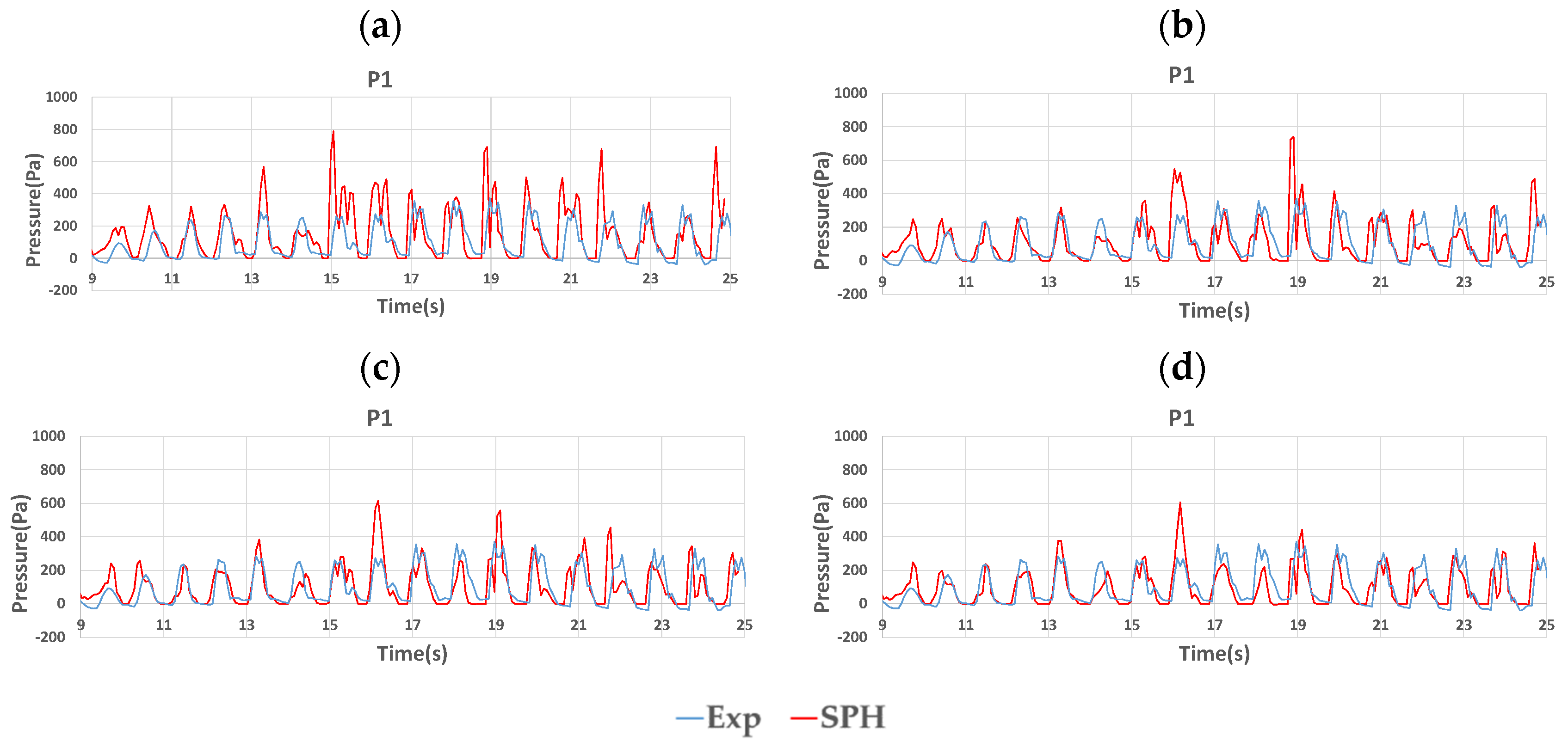
The speed of sound plays an important role in WCSPH. However, an artificially reduced value is commonly used to avoid excessive computational cost because an increase in speed requires a shorter time step, which increases total computation time. Using a reduced value for the speed of sound could result in less accurate results for impact pressure problems. Therefore, in this study, 3D single-phase SPH simulations using different values for the speed of sound were executed to determine the minimum adequate value. Figure 6a presents a pressure comparison for P1 under roll oscillations. The selected coefsound values were 20, 40, 60, and 80. Coefsound of 80 provides the best results, but increases computation time by four times compared to a coefsound of 20. To balance accuracy and computation time, a coefsound of 60 was selected in this study.
The natural frequencies of the prismatic tank with different filling ratios were calculated using Equations (21) and (22) (see Table 5). To validate SPH for violent sloshing, the frequency of external oscillation should be close to the natural frequency of the tank. Therefore, values of f = 1.08 Hz and 1.04 Hz were selected for sway and roll oscillations, respectively, at a filling ratio of 25%. Additionally, the maximum amplitude was selected for the validation of each external motion. In this condition, the computation time for 30 seconds of simulation time was 347 hours.
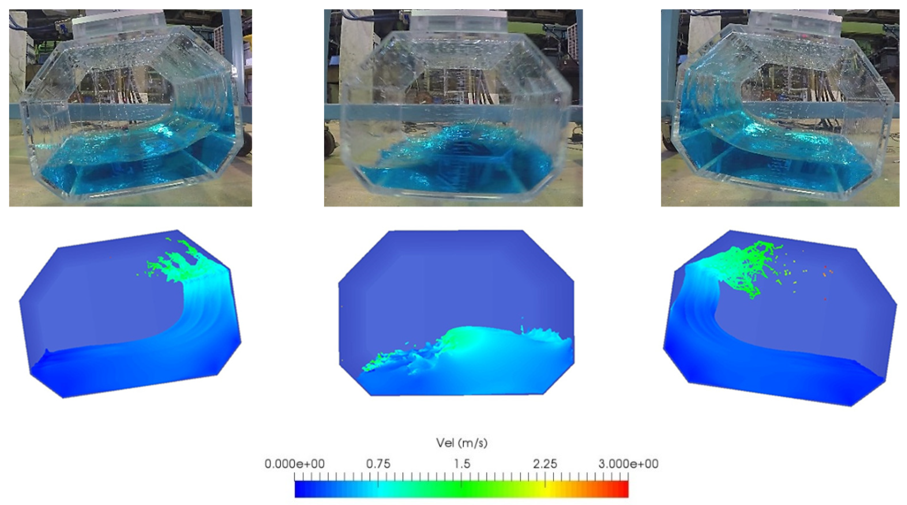
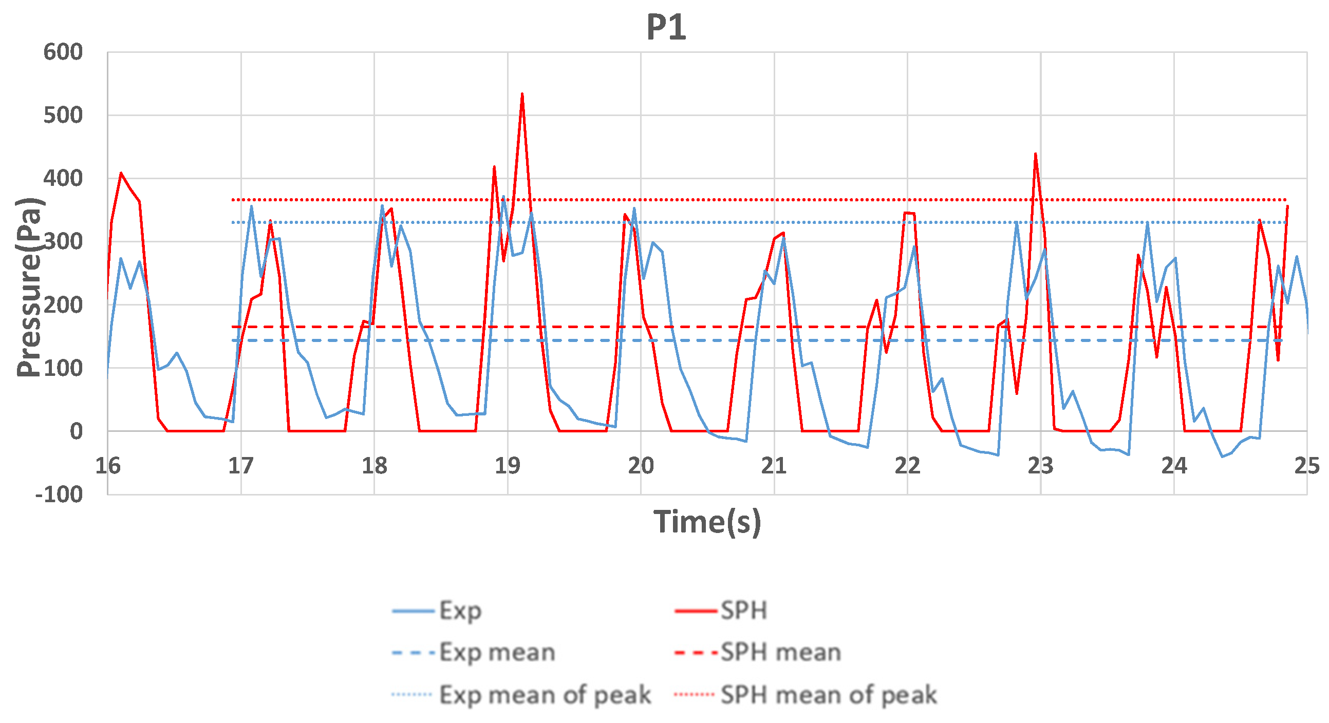
Figure 7 presents a comparison of free surface evolutions under sway oscillations. In this moderate sloshing situation, single-phase SPH can accurately reproduce the resonance of the fluid and free surface deformation. Figure 8 presents a comparison of free surface evolutions under roll oscillations. With this type of oscillation, the fluid motion in the tank becomes more violent, as shown in Figure 8, and the water front touches the top of the tank. The SPH simulation accurately reproduces the run-up, breaking, and splashing phenomena during sloshing, but the water does not reach the top of the tank. This could be because the smoothing scheme and artificial viscosity used in SPH led to slightly greater dissipation compared to the real physics. Figure 9 and Figure 10 present comparisons of pressure variation over time at P1 between the SPH and experimental results. In these graphs, the arithmetic means of pressure and peak pressure are drawn together. The dashed line represents the arithmetic mean of pressure and the dotted line represents the mean of peak pressure under each oscillation type over nine cycles. The results reveal that the mean pressure and the mean of peak pressure are overestimated by SPH for both sway and roll oscillations, even though over 10 million particles were used. Additionally, one can see that the fluctuation in peak pressure in the SPH results is more prominent than that in the experimental results.
5.2. 2D Two-Phase SPH Simulation
As described in the previous subsection, a 3D single-phase SPH method was applied to the prediction of sloshing in a prismatic tank. As a result, the violent resonance of fluid with complex free surface excitation caused by external sway and roll was qualitatively reproduced with an accurate impact pressure near the tank’s corners. However, the simulated results did diverge from the experimental results, especially the pressure peak values, even while using over 10M particles. To identify possible elements for reducing these discrepancies, the two-phase SPH simulation was performed under the same conditions to analyze the influence of air phase on sloshing in a prismatic tank. The application of two-phase SPH was reported by Mokos et al. [47,56] and a ratio of the speeds of sound in liquid and gas phases of 7.5 had good agreement with experimental results [56]. In this study, the speed of sound of water was determined to maintain a ratio above 7.0 when considering the real speed of sound in air (i.e., 343 m/s). For the sake of a fair comparison and a clear discussion of the effects of the air phase, a 2D simulation using a single-phase SPH method with the same particle spacing as the previous simulation was performed. The computation time for two-phase SPH simulation is much greater than for the single-phase SPH simulation because air particles must be calculated in addition to water particles. Additionally, the minimum time step satisfying the Mach number becomes smaller based on the greater speed of sound. As a result, it is infeasible to run 3D two-phase SPH for sloshing simulations with a large number of particles. However, it is not suitable to use a different particle spacing value and parameters for two-phase SPH when comparing the results to those of single-phase SPH. Therefore, we decided to run 2D sloshing simulations based on two-phase SPH using a consistent particle spacing of 0.8 mm. This is a reasonable choice because pure sway and pure roll motions were introduced in the experiment, which means the flows in the tank can be regarded as 2D, rather than 3D. These assumptions led to a reduction in the total number of particles to 90,057 for 2D two-phase SPH simulation at a filling ratio of 25%.
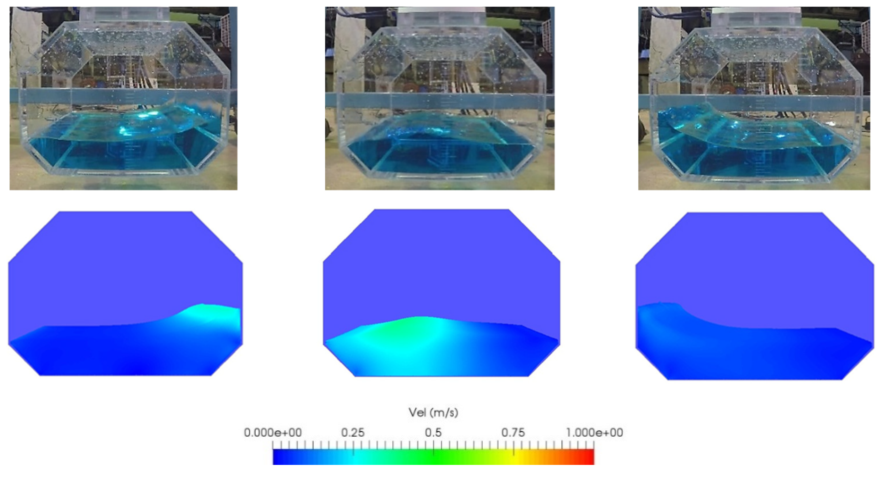
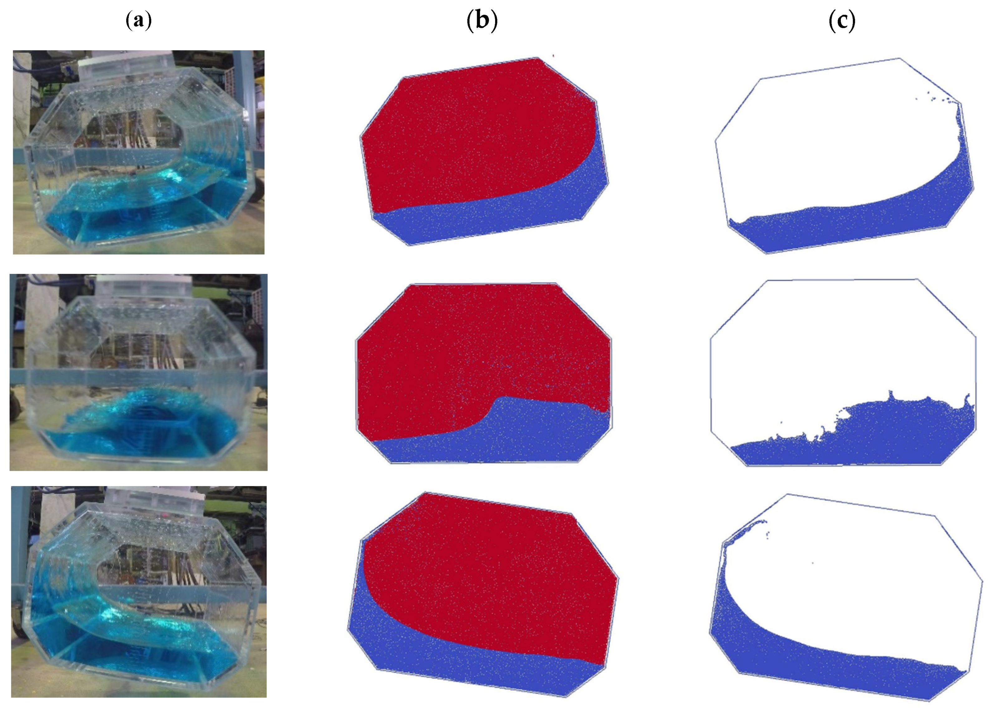
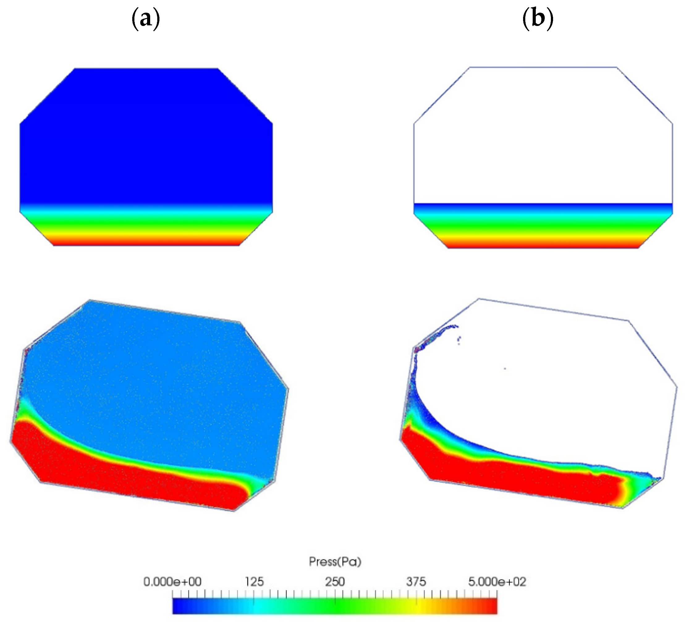
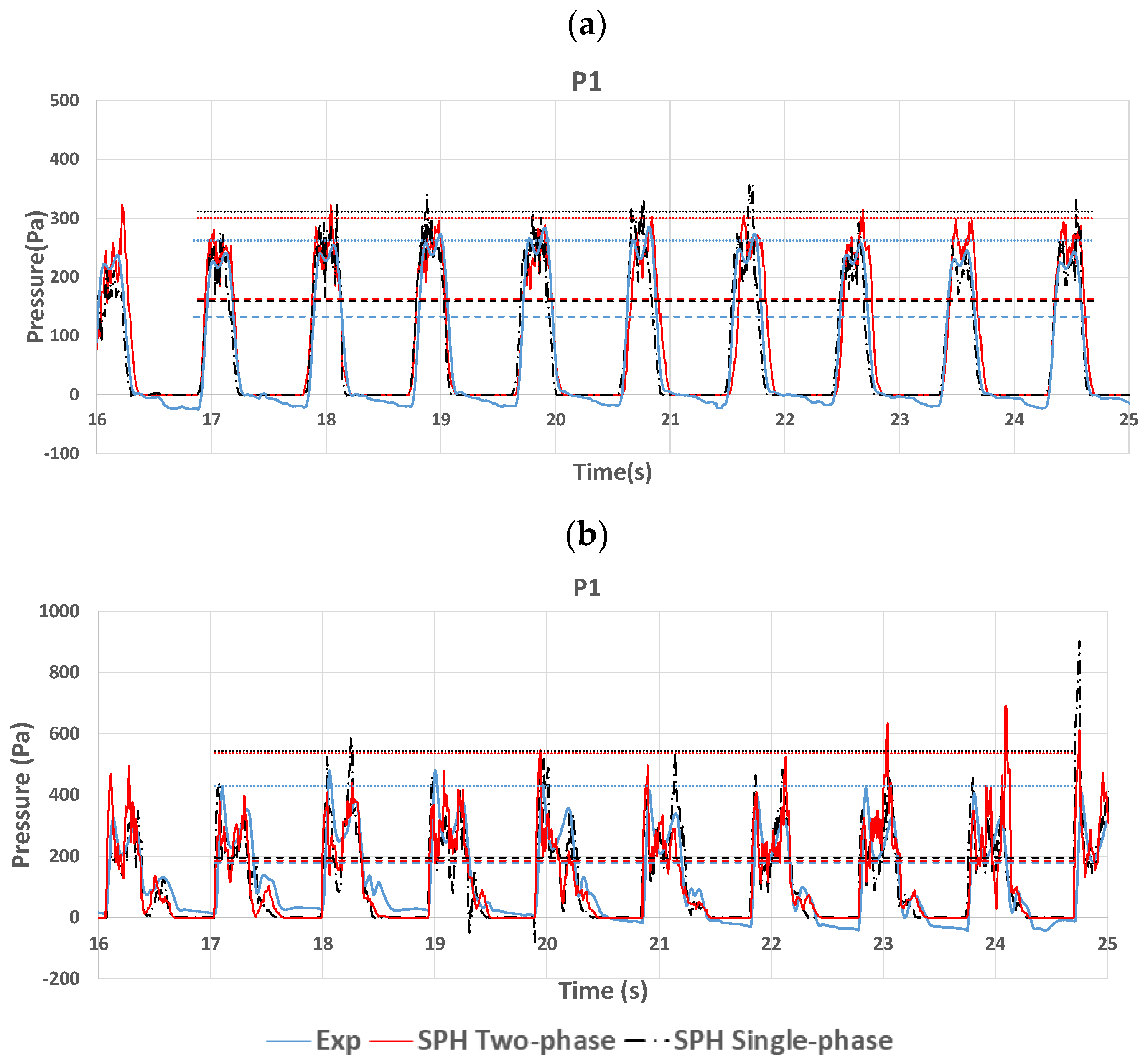
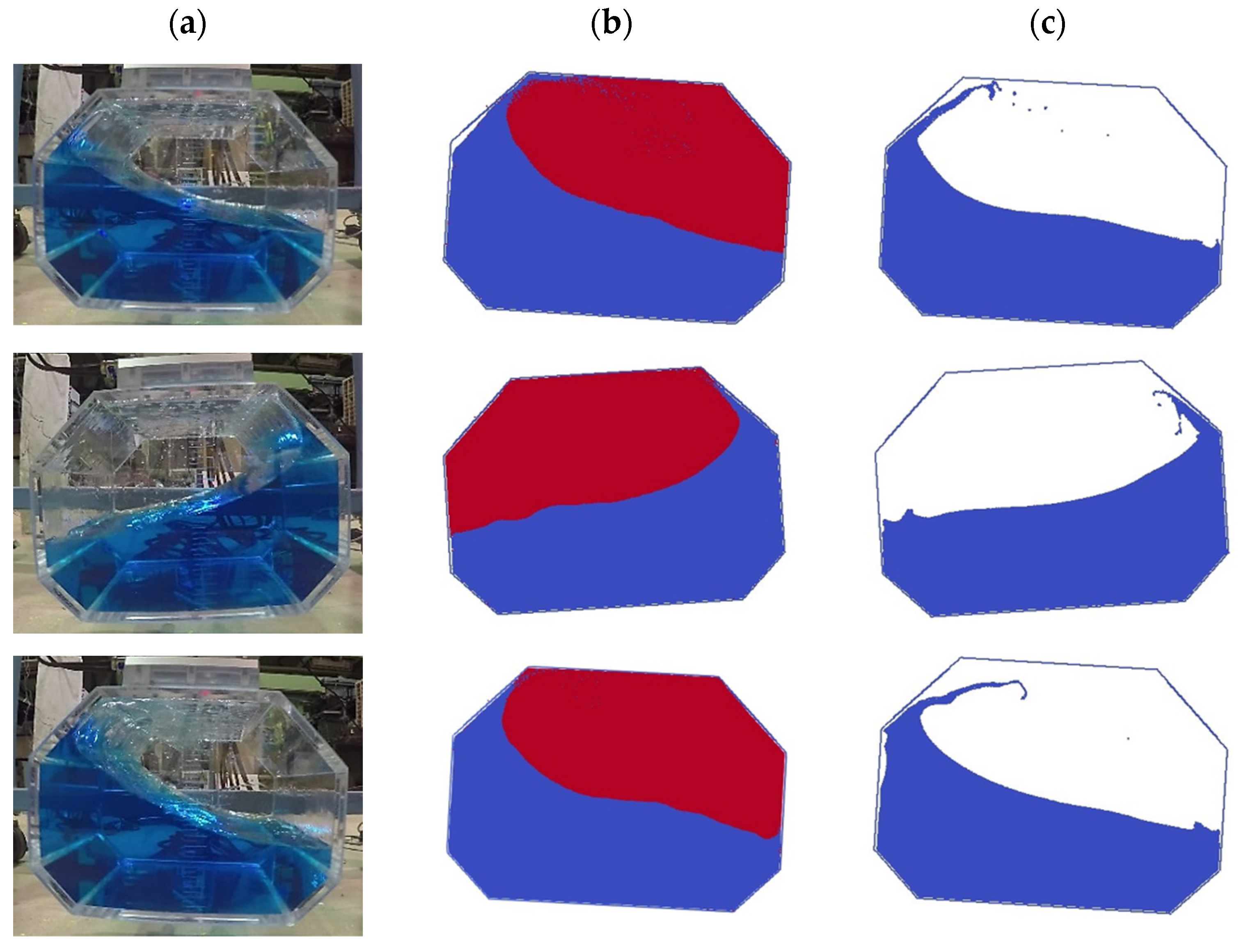
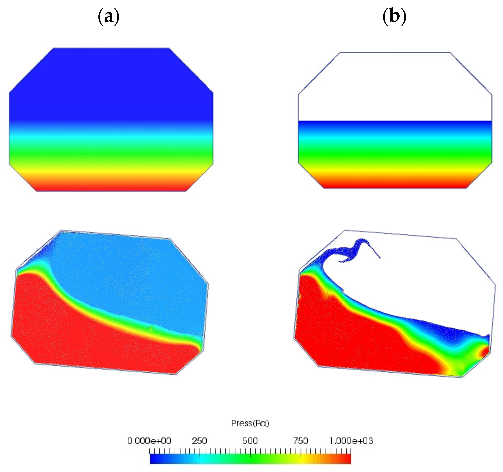
Table 6 lists the parameters used for two-phase SPH simulation. As mentioned previously, the speed of sound has a significant influence on impact pressure and the ratio of the speeds of sound between air and water is important from the perspective of numerical stability. Figure 11 presents comparisons of the free surface evolutions between single-phase and two-phase SPH, as well as the experimental results. The computation time for 30 s of simulation time was 81 hours for two-phase and 9 hours for single-phase SPH simulations, respectively. In the results for two-phase simulation, the red-colored region is the air phase and the blue-colored region is the water phase. Two-phase SPH exhibits a smoother free surface shape compared to single-phase SPH. This could be because the number of neighboring particles near the free surface is increased with the inclusion of air particles. The two-phase simulation shows better agreement with the experimental results, especially in terms of the run-up along the side wall. The single-phase simulation tends to exhibit less run-up and the fluid easily detaches from the side wall based on the exclusion of an air phase. Figure 12 presents the pressure contours under static and dynamic conditions for a filling ratio of 25% under roll oscillation. One can see that both SPH simulations yield smooth hydrostatic pressure contours [14], but the two-phase SPH exhibits a smoother pressure distribution under dynamic conditions. In SPH, flow is simulated by solving partial differential equations locally with a compact support. However, the pressure field can be naturally smoothed over the entire liquid domain. Figure 13 presents a comparison of local pressure at P1 for sway and roll oscillations. The peak values tend to be overestimated by both single-phase and two-phase SPH. The mean value is also overestimated for sway, but good agreement can be observed for the roll. In general, the mean peak pressure is slightly more accurate for two-phase SPH. It is known that pressure fields generally exhibit oscillation based on the effects of density fluctuation in WCSPH, but pressure fluctuation is also suppressed by taking the air phase into account. The shape of the pressure curve, especially the tail of the pressure curve after the peak, shows better agreement with the experimental results for roll for two-phase SPH. It should be noted that the single-phase 2D SPH results show better agreement with the experimental results compared to the single-phase 3D SPH results in Figure 9 and Figure 10, even though the same particle spacing is used. This implies that the accuracy of 3D simulation tends to be worse than that of 2D simulation. The SPH method adopts a Lagrangian formulation, so a uniform distribution over time is an important element for the accurate analysis of flows. This uniform distribution might be more difficult to maintain in 3D simulations when compared to 2D simulations.
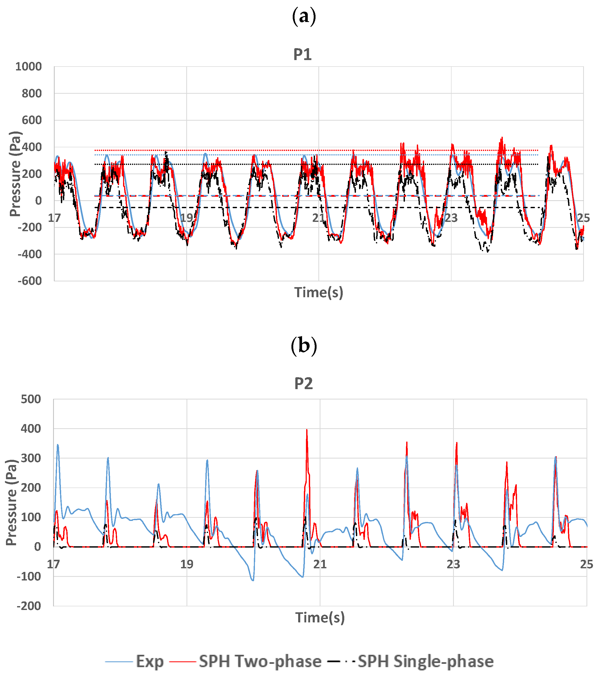
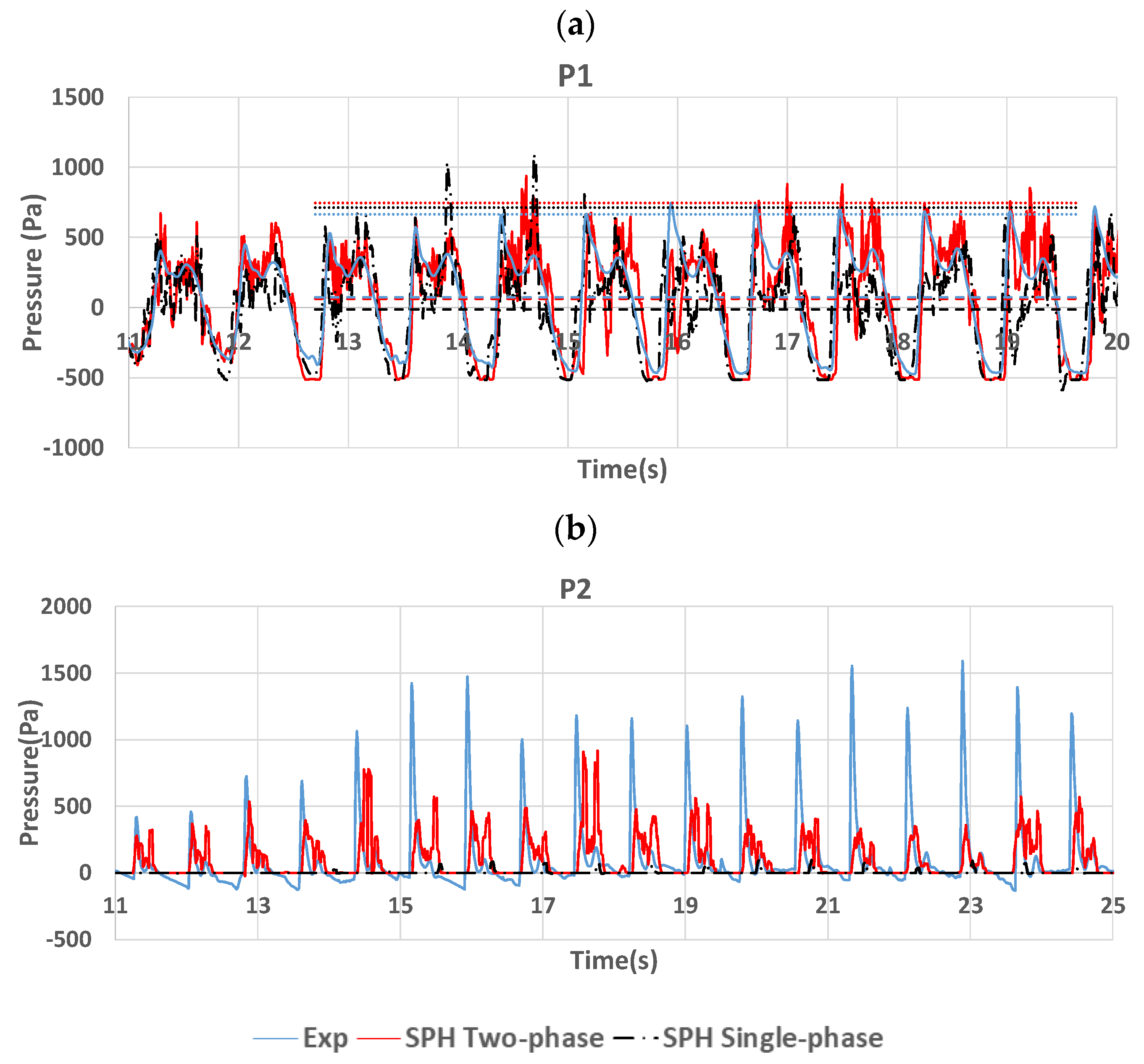
Figure 14 presents images of free surface evolution under roll oscillation with f =1.30 Hz and A = 8.66° for a filling ratio of 50%. For two-phase SPH, the front shape of the run-up can be maintained along the side wall and touches the top wall, which is similar to the experimental observations. In contrast, for single-phase SPH, the fluid easily detaches from the side wall, similar to the filling ratio of 25%. Figure 15 presents the pressure contours under static and dynamic conditions. A smoother pressure distribution can again be observed in the liquid phase for two-phase SPH and one can see that the presence of air clearly affects the behavior of liquids, especially in terms of run-up and spraying. Figure 16 presents a comparison of the local pressures at P1 and P2 under sway oscillation with f = 1.34 Hz and A = 6.52 mm at a filling ratio of 50%. In the two-phase SPH results, the arithmetic mean of pressure shows reasonable agreement with the experimental results and the mean of peak pressure also shows reasonable agreement at P1, whereas single-phase SPH failed to predict these values accurately. The prediction accuracy of pressure at P2 is poor because the pressure at this point is relatively spikey when compared to that at P1. However, the two-phase SPH results show much better agreement with the experimental results than the single-phase SPH results at P2. A similar trend of improvement in terms of pressure accuracy can be observed for the roll oscillation shown in Figure 17. The accuracy of peak pressure at P2 is worse than that in the sway case because the flow inside the tank is more violent and the impact pressure is much greater than that in the sway case. However, the importance of the air phase is clearly demonstrated because single-phase SPH cannot capture the impact pressure at all.
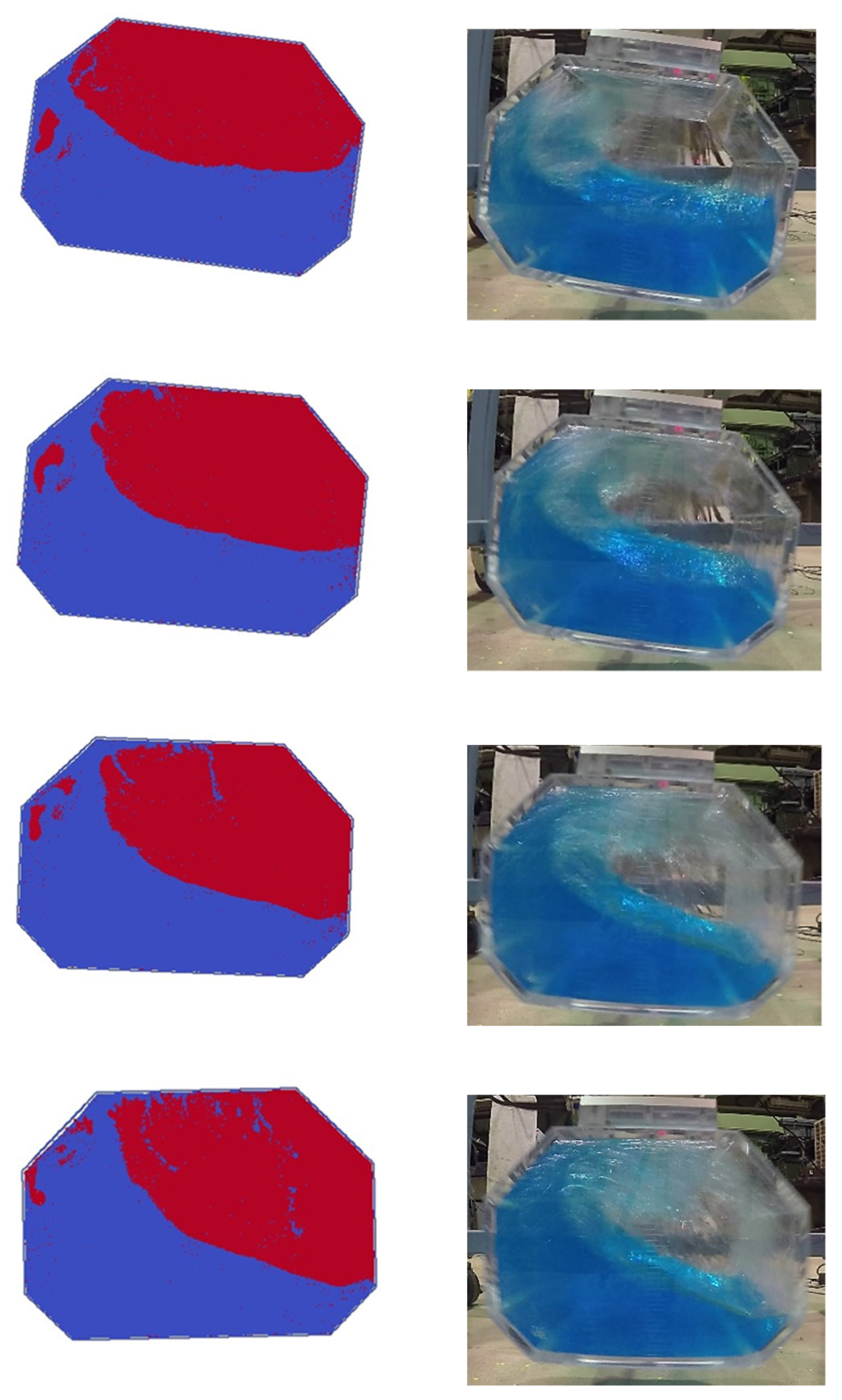
Figure 18 presents comparisons between the two-phase SPH results and experimental results under roll oscillation. The intension for this comparison is to highlight the air and water mixing that occurs during violent sloshing. In the two-phase SPH simulation, the existence of air pockets and an air-water mixture is captured, which matches the experiment. This is one of the major advantages of two-phase flow simulations in terms of deep discussion of the sloshing phenomenon itself. Mokos et al. [56] detailed the issue of air mixture creation and void creation in a two-phase flow. It is clear that much finer particle spacing is required to capture the creation process of air-water mixtures quantitatively. Further studies for the detailed analysis of air effects using a large number of particles are expected. In addition, for the engineering standpoints, it is expected to couple two-phase SPH with a mathematical model for ship motion to carry out fully coupled ship-tank simulations, which is similar to those discussed in References [57,58,59,60].
6. Conclusions
In this paper, single and two-phase SPH simulations accelerated by a GPU were performed to analyze sloshing in a tank. For quantitative validation, a dedicated sloshing experiment was conducted using a realistically shaped prismatic tank that was subjected to external sway and roll oscillations. The experiment was successful, and fluid behavior and impact pressure at three different locations were measured. Next, single-phase 3D SPH simulations were performed with several particle distances. It was confirmed that 0.8 mm of particle spacing is necessary to capture the shape of pressure variation. It was also confirmed that the speed of sound has a significant influence on the impact pressure and pressure oscillation. By comparing the simulation results to the experimental results, it was demonstrated that large-scale single-phase SPH, using over 10 million particles, fails to represent free surface evolution and impact pressure accurately. Next, a 2D two-phase simulation was performed and validated by comparing its results to the experimental results, as well as those of the two-dimensional single-phase SPH simulation. Based on comparisons under different conditions, the importance of an air phase in sloshing phenomena was clarified and improvement of impact pressure simulation accuracy near the tank corners in terms of mean and peak pressures was confirmed.
Author Contributions
Conceptualization, H.H. Simulation, A.T. Experiment, A.M. and H.H. Validation: A.T. and H.H. Discussion, A.T. and H.H. Writing and editing, A.T. and H.H.
Funding
This work was supported by JSPS KAKENHI Grant number 16H03135.
Acknowledgments
The authors wish to thank the Directorate General of Resources for Sciences, Technology, and Higher Education of the Ministry of Research, Technology, and Higher Education of the Republic Indonesia for BPP-LN doctoral scholarship No. 181.47/E4.4/2014. The authors also thank Dr. Yuuki Taniguchi for his technical assistance with the experiments.
Conflicts of Interest
The authors declare no conflicts of interest. The funders had no role in the design of the study or in the collection, analysis, or interpretation of data, nor in the writing of the manuscript or the decision to publish the results.
References
- Kishev, Z.R.; Hu, C.; Kashiwagi, M. Numerical simulation of violent sloshing by a CIP-based method. J. Mar. Sci. Technol. 2006, 11, 111–122. [Google Scholar] [CrossRef]
- Kim, Y. Numerical simulation of sloshing flows with impact load. Appl. Ocean Res. 2001, 23, 53–62. [Google Scholar] [CrossRef]
- Jiang, S.C.; Teng, B.; Bai, W.; Ying, G. Numerical simulation of coupling effect between ship motion and liquid sloshing under wave action. Ocean Eng. 2015, 108, 140–154. [Google Scholar] [CrossRef]
- Chen, Y.; Xue, M. Numerical simulation of liquid sloshing with different filling levels using openFOAM and experimental validation. Water 2018, 10, 1752. [Google Scholar] [CrossRef]
- Lucy, L.A. Numerical approach to the testing of the fission hypothesis. Astron. J. 1977, 82, 1013–1024. [Google Scholar] [CrossRef]
- Gingold, R.A.; Monaghan, J.J. Smoothed Particle Hydrodynamics: Theory and Application to Non-Spherical Stars. Mon. Not. R. Astron. Soc. 1977, 181, 375–389. [Google Scholar] [CrossRef]
- Monaghan, J.J. Simulating free surface flows with SPH. J. Comput. Phys. 1994, 110, 399–406. [Google Scholar] [CrossRef]
- Dalrymple, R.A.; Rogers, B.D. Numerical modelling of water waves with the SPH method. Coast. Eng. 2006, 53, 141–147. [Google Scholar] [CrossRef]
- Makris, C.V.; Memos, C.D.; Krestenitis, Y.N. Numerical modeling of surf zone dynamics under weak plunging breakers with SPH method. Ocean Model. 2016, 98, 12–35. [Google Scholar] [CrossRef]
- Antuono, M.; Colagrossi, A.; Marrone, S.; Lugni, C. Propagation of gravity waves through an SPH scheme with numerical diffusive terms. Comput. Phys. Commun. 2011, 182, 866–877. [Google Scholar] [CrossRef]
- Altomare, C.; Dominguez, J.M.; Crespo, A.J.C.; Gonzalez-Cao, J.; Suzuki, T.; Gómez-Gesteira, M.; Troch, P. Long-crested wave generation and absorption for SPH-based DualSPHysics model. Coast. Eng. 2017, 127, 37–54. [Google Scholar] [CrossRef]
- Lind, S.J.; Xu, R.; Stanby, P.K.; Rogers, B.D. Incompressible smoothed particle hydrodynamics for free surface flow: A generalized diffusion-based algorithm for stability and validations for impulsive flows and propagating waves. J. Comput. Phys. 2012, 231, 1499–1523. [Google Scholar] [CrossRef]
- Colagrossi, A.; Souto-Iglesias, A.; Antuono, M.; Marrone, S. Smoothed-particle- hydrodynamics modeling of dissipation mechanisms in gravity waves. Phys. Rev. E 2013, 87, 023302. [Google Scholar] [CrossRef] [PubMed]
- Trimulyono, A.; Hashimoto, H. Experimental validation of smoothed particle hydrodynamics on generation and propagation on water waves. J. Mar. Sci. Eng. 2019, 7, 17. [Google Scholar] [CrossRef]
- Antoci, C.; Gallati, M.; Sibilla, S. Numerical simulation of fluid-structure interaction by SPH. Comput. Struct. 2007, 85, 879–890. [Google Scholar] [CrossRef]
- Crespo, A.J.C.; Gómez-Gesteira, M.; Dalrymple, R.A. 3D SPH simulation of large waves mitigation with a dike. J. Hydraul. Res. 2007, 45, 631–642. [Google Scholar] [CrossRef]
- Altomare, C.; Crespo, A.J.C.; Dominguez, J.M.; Gómez-Gesteira, M.; Suzuki, T.; Verwaest, T. Applicability of smoothed particle hydrodynamics for estimation of sea wave impact on coastal structures. Coast. Eng. 2015, 96, 1–12. [Google Scholar] [CrossRef]
- Barreiro, A.; Crespo, A.J.C.; Dominguez, J.M.; Gómez-Gesteira, M. Smoothed Particle Hydrodynamics for coastal engineering problems. Comput. Struct. 2013, 120, 96–106. [Google Scholar] [CrossRef]
- Wei, Z.; Dalrymple, R.A.; Hérault, A.; Bilotta, G.; Rustico, E.; Yeh, H. SPH modeling of dynamic impact of tsunami bore on bridge piers. Coast. Eng. 2015, 104, 26–42. [Google Scholar] [CrossRef]
- Sarfaraz, M.; Park, A. SPH numerical simulation of tsunami wave forces impinged on bridge superstructures. Coast. Eng. 2017, 121, 145–157. [Google Scholar] [CrossRef]
- Marrone, S.; Colagrossi, A.; Antuono, M.; Colicchio, G.; Graziani, G. An accurate SPH modeling of viscous flows around bodies at low and moderate Reynolds numbers. J. Comput. Phys. 2013, 245, 456–475. [Google Scholar] [CrossRef]
- Zisis, I.; Messahel, R.; Boudlal, A.; Linden, B.; Koren, B. Validation of robust SPH schemes for fully compressible multiphase flows. Int. J. Multiphys. 2015, 9, 225–234. [Google Scholar] [CrossRef]
- Kawamura, K.; Hashimoto, H.; Matsuda, A.; Terada, D. SPH Simulation of ship behaviour in severe water-shipping situations. Ocean Eng. 2016, 120, 220–229. [Google Scholar] [CrossRef]
- Gómez-Gesteira, M.; Cerqueiro, D.; Crespo, A.J.C.; Dalrymple, R.A. Green water overtopping with a SPH model. Ocean Eng. 2005, 32, 223–238. [Google Scholar] [CrossRef]
- Le Touzé, D.; Marsh, A.; Oger, G.; Guilcher, P.M.; Khaddaj-Mallat, C.; Alessandrini, B.; Ferrant, P. SPH Simulation of green water and ship flooding scenarios. J. Hydrodyn. B 2010, 22, 231–236. [Google Scholar] [CrossRef]
- Tafuni, A.; Dominguez, J.M.; Vacondio, R.; Crespo, A.J.C. A versatile algorithm for the treatment of open boundary conditions in Smoothed particle hydrodynamics GPU models. Comput. Methods Appl. Mech. Eng. 2018, 342, 604–624. [Google Scholar] [CrossRef]
- Gonzalez-Cao, J.; Altomare, C.; Crespo, A.J.C.; Dominguez, J.M.; Gómez-Gesteira, M.; Kisacik, D. On the accuracy of DualSPHysics to assess violent collision with coastal structures. Comput. Fluids 2019, 179, 604–612. [Google Scholar] [CrossRef]
- Verbrugghe, T.; Dominguez, J.M.; Altomare, C.; Tafuni, A.; Vacondio, R.; Troch, P.; Kortenhaus, A. Non-linear wave generation and absorption using open boundaries within DualSPHysics. Comput. Phys. Commun. 2019, 240, 46–59. [Google Scholar] [CrossRef]
- Delorme, L.; Colagrossi, A.; Souto-Iglesias, A.; Zamora-Rodrigues, R.; Botia-Vera, E. A set of canonical problems in sloshing, Part I: Pressure field in forced roll-comparison between experimental results and SPH. Ocean Eng. 2009, 36, 168–178. [Google Scholar] [CrossRef]
- Landrini, M.; Colagrossi, A.; Faltinsen, O.M. Sloshing in 2-D flows by the SPH method. In Proceedings of the 8th numerical ship hydrodynamics, Busan, Korea, 22–25 September 2003. [Google Scholar]
- Chen, Z.; Zong, Z.; Li, H.T.; Li, J. An investigation into the pressure on solid walls in 2D sloshing using SPH method. Ocean Eng. 2013, 59, 129–141. [Google Scholar] [CrossRef]
- Kim, Y. Experimental and numerical analyses of sloshing flows. J. Eng. Math. 2007, 58, 191–210. [Google Scholar] [CrossRef]
- Colagrossi, A.; Lugni, C.; Brocchini, M. A study of violent sloshing impacts using an improved SPH method. J. Hydraul. Res. 2010, 48, 94–104. [Google Scholar] [CrossRef]
- Shao, J.R.; Li, H.Q.; Liu, G.R.; Liu, M.B. An improved SPH method for modeling liquid sloshing dynamics. Comput. Struct. 2012, 100, 18–26. [Google Scholar] [CrossRef]
- Rafiee, A.; Pistani, F.; Thiagarajan, K. Study of liquid sloshing: Numerical and experimental approach. Comput. Mech. 2011, 47, 65–75. [Google Scholar] [CrossRef]
- Bouscasse, B.; Antuono, M.; Colagrossi, A.; Lugni, C. Numerical and experimental investigation of nonlinear shallow water sloshing. Int. J. Nonlinear Sci. Numer. Simul. 2013, 14, 123–138. [Google Scholar] [CrossRef]
- De Chowdhury, S.; Sannasiraj, S.A. Numerical simulation of 2D sloshing waves using SPH with diffusive term. Appl. Ocean Res. 2014, 47, 219–240. [Google Scholar] [CrossRef]
- Green, D.M.; Peiro, J. Long duration SPH simulations of sloshing in tanks with a low fill ratio and high stretching. Comput. Fluids 2018, 174, 179–199. [Google Scholar] [CrossRef]
- Crespo, A.J.C.; Domínguez, J.M.; Rogers, B.D.; Gómez-Gesteira, M.; Longshaw, S.; Canelas, R.; García-Feal, O. DualSPHysics: Open-Source Parallel CFD solver based on smoothed particle hydrodynamics (SPH). Comput. Phys. Commun. 2015, 187, 204–216. [Google Scholar] [CrossRef]
- Crespo, A.J.C.; Domínguez, J.M.; Barreiro, A.; Gómez-Gesteira, M.; Rogers, B.D. GPUs, a new tool of acceleration in CFD: Efficiency and reliability on smoothed particle hydrodynamics. PLoS ONE 2011, 6, e20685. [Google Scholar] [CrossRef]
- Domínguez, J.M.; Crespo, A.J.C.; Valdez-Balderas, D.; Rogers, B.D. New multi-GPU implementation for smoothed particle hydrodynamics on heterogeneous clusters. Comput. Phys. Commun. 2013, 184, 1848–1860. [Google Scholar] [CrossRef]
- Violeau, D. Fluid Mechanics and the SPH Method: Theory and Applications; Oxford University Press: Oxford, UK, 2012. [Google Scholar]
- Liu, G.R.; Liu, M.B. Smoothed Particle Hydrodynamics: A Meshfree Particle Method; World Scientific: Singapore, 2003. [Google Scholar]
- Cao, X.Y.; Ming, F.R.; Zhang, A.M. Sloshing in a rectangular tank based on SPH simulation. Appl. Ocean Res. 2014, 47, 241–254. [Google Scholar] [CrossRef]
- Wendland, H. Piecewise Polynomial, Positive Definite and Compactly Supported Radial Functions of Minimal Degree. Adv. Comput. Math. 1995, 4, 389–396. [Google Scholar] [CrossRef]
- Colagrossi, A.; Landrini, M. Numerical simulation of interfacial flows by smoothed particle hydrodynamics. J. Comput. Phys. 2003, 192, 448–475. [Google Scholar] [CrossRef]
- Mokos, A.; Rogers, B.D.; Stansby, P.K.; Domínguez, J.M. Multi-phase modelling of violent hydrodynamics on GPUs. Comput. Phys. Commun. 2015, 196, 304–316. [Google Scholar] [CrossRef]
- Monaghan, J.J. Smoothed particle hydrodynamics. Annu. Rev. Astron. Astrophys. 1992, 110, 543–574. [Google Scholar] [CrossRef]
- Molteni, D.; Colagrossi, A. A simple procedure to improve the pressure evaluation in hydrodynamic context using the SPH. Comput. Phys. Commun. 2009, 180, 861–872. [Google Scholar] [CrossRef]
- Antuono, M.A.; Colagrossi, A.; Marrone, S.; Molteni, D. Free-surface flows solved by means of SPH schemes with numerical diffusive term. Comput. Phys. Commun. 2010, 181, 532–549. [Google Scholar] [CrossRef]
- Antuono, M.A.; Colagrossi, A.; Marrone, S. Numerical diffusive term in weakly-compressible SPH schemes. Comput. Phys. Commun. 2012, 183, 2570–2580. [Google Scholar] [CrossRef]
- Leimkuhler, B.J.; Reich, S.; Skeel, R.D. Integration Methods for Molecular dynamics. In Mathematical Approaches to Biomolecular Structure and Dynamics; The IMA Volumes in Mathematics and its Applications, 82; Mesirov, J.P., Schulten, K., Sumners, D.W., Eds.; Springer: New York, NY, USA, 1996. [Google Scholar]
- Monaghan, J.J.; Kos, A. Solitary Waves on a Cretan Beach. J. Waterw. Port Coast. Ocean Eng. 1999, 125, 145–155. [Google Scholar] [CrossRef]
- Crespo, A.J.C.; Gomes-Gesteira, M.; Dalrymple, R.A. Boundary Conditions Generated by Dynamic Particles in SPH Methods. Comput. Mater. Contin. 2007, 5, 173–184. [Google Scholar]
- Faltinsen, O.M.; Timokha, A.N. Sloshing; Cambridge University Press: New York, NY, USA, 2009. [Google Scholar]
- Mokos, A.; Rogers, B.D.; Stansby, P.K. A Multi-phase particle shifting algorithm for SPH simulations of violent hydrodynamics with a large number of particles. J. Hydraul. Res. 2016, 55, 143–162. [Google Scholar] [CrossRef]
- Du, Y.; Wang, C.; Zhang, N. Numerical simulation on coupled ship with nonlinear sloshing. Ocean Eng. 2019, 178, 493–500. [Google Scholar] [CrossRef]
- Saripilli, R.J.; Sen, D. Numerical studies on effects of slosh coupling on ship motions and derived slosh load. Appl. Ocean Res. 2018, 76, 71–87. [Google Scholar] [CrossRef]
- Servan-Camas, B.; Cercos-Pita, J.L.; Colom-Cobb, J.; Garcia-Espinosa, J.; Sauto-Iglesias, A. Time domain simulation of coupled sloshing-seakeeping problems by SPH-FEM coupling. Ocean Eng. 2016, 123, 383–396. [Google Scholar] [CrossRef]
- Hashimoto, H.; Ito, Y.; Kawakami, N.; Sueyoshi, M. Numerical simulation method for coupling of tank fluid and ship roll motions. In Proceedings of the 11th international conference on the stability of ships and ocean vehicles (STAB 2012), Athens, Greece, 23–28 September 2012; pp. 477–486. [Google Scholar]
Figure 1.
(a) Overview of the forced oscillation machine for sloshing tests and (b) a photograph of the prismatic tank.
Figure 1.
(a) Overview of the forced oscillation machine for sloshing tests and (b) a photograph of the prismatic tank.

Figure 2.
Geometry of the prismatic tank and locations of external gauges (units in meters).

Figure 3.
Time histories of forced oscillation motions with maximum amplitudes (a) sway, (b) heave, (c) roll, and (d) yaw.
Figure 3.
Time histories of forced oscillation motions with maximum amplitudes (a) sway, (b) heave, (c) roll, and (d) yaw.

Figure 4.
Measured pressure at P1 with a filling ratio of 25% for (a) sway and (b) roll motions.

Figure 5.
Convergence of dynamic pressure with respect to particle spacing for sway oscillations with f = 1.08 Hz and A = 6.52 mm.
Figure 5.
Convergence of dynamic pressure with respect to particle spacing for sway oscillations with f = 1.08 Hz and A = 6.52 mm.

Figure 6.
Influence of the speed of sound on hydrodynamic pressure: coefsound = (a) 20, (b) 40, (c) 60, and (d) 80.
Figure 6.
Influence of the speed of sound on hydrodynamic pressure: coefsound = (a) 20, (b) 40, (c) 60, and (d) 80.

Figure 7.
Free surface evolution under sway oscillations at t = 9.8 seconds, 10.0 seconds, and 10.2 seconds with a 25% filling ratio.
Figure 7.
Free surface evolution under sway oscillations at t = 9.8 seconds, 10.0 seconds, and 10.2 seconds with a 25% filling ratio.

Figure 8.
Free surface evolution under roll oscillations at t = 11.0 seconds, 11.2 seconds, and 11.4 seconds with a 25% filling ratio.
Figure 8.
Free surface evolution under roll oscillations at t = 11.0 seconds, 11.2 seconds, and 11.4 seconds with a 25% filling ratio.

Figure 9.
Impact pressure under sway excitation with a particle spacing of 0.8 mm at a 25% filling ratio.
Figure 9.
Impact pressure under sway excitation with a particle spacing of 0.8 mm at a 25% filling ratio.

Figure 10.
Impact pressure under roll excitation with a particle spacing 0.8 mm at a 25% filling ratio.
Figure 10.
Impact pressure under roll excitation with a particle spacing 0.8 mm at a 25% filling ratio.

Figure 11.
Free surface evolution under roll oscillation in (a) the experiment, (b) two-phase SPH, and (c) single-phase SPH with a filling ratio of 25% at t = 11.0 s, 11.2 s, and 11.4 s.
Figure 11.
Free surface evolution under roll oscillation in (a) the experiment, (b) two-phase SPH, and (c) single-phase SPH with a filling ratio of 25% at t = 11.0 s, 11.2 s, and 11.4 s.

Figure 12.
Pressure contour under roll oscillation for (a) two-phase SPH and (b) single-phase SPH at t = 0.0 seconds and 11.4 seconds.
Figure 12.
Pressure contour under roll oscillation for (a) two-phase SPH and (b) single-phase SPH at t = 0.0 seconds and 11.4 seconds.

Figure 13.
Comparison of pressure at P1 for (a) sway and (b) roll with a filling ratio of 25%.

Figure 14.
Free surface evolution of roll excitation in (a) the experiment, (b) two-phase, and (c) single-phase SPH with t = 3.6 seconds, 3.9 seconds, and 4.4 seconds.
Figure 14.
Free surface evolution of roll excitation in (a) the experiment, (b) two-phase, and (c) single-phase SPH with t = 3.6 seconds, 3.9 seconds, and 4.4 seconds.

Figure 15.
Pressure contours with a filling ratio of 50% for (a) two-phase and (b) single-phase SPH with t = 0.0 seconds and 12.15 seconds.
Figure 15.
Pressure contours with a filling ratio of 50% for (a) two-phase and (b) single-phase SPH with t = 0.0 seconds and 12.15 seconds.

Figure 16.
Comparison of pressures at (a) P1 and (b) P2 for sway oscillation with a filling ratio of 50%.
Figure 16.
Comparison of pressures at (a) P1 and (b) P2 for sway oscillation with a filling ratio of 50%.

Figure 17.
Comparison of pressures at (a) P1 and (b) P2 under roll oscillation with a filling ratio of 50%.
Figure 17.
Comparison of pressures at (a) P1 and (b) P2 under roll oscillation with a filling ratio of 50%.

Figure 18.
Images of air-water mixture under roll oscillation with a filling ratio of 50% at t = 16.15 seconds, 16.20 seconds, 16.25 seconds, and 16.30 seconds.
Figure 18.
Images of air-water mixture under roll oscillation with a filling ratio of 50% at t = 16.15 seconds, 16.20 seconds, 16.25 seconds, and 16.30 seconds.


Table 1.
Experimental conditions.
| External Motion | Frequency (Hz) | Amplitude (mm/deg) |
|---|---|---|
| Sway | 1.08 | 0.82, 1.63, 3.26, 6.52 |
| 1.34 | ||
| Roll | 1.04 | 1.09, 2.17, 4.33, 8.66 |
| 1.34 | ||
| Heave | 1.04 | 2.85, 5.7 |
| 1.34 | ||
| Yaw | 1.08 | 3.0 |
| 1.34 |
Table 2.
Dimensions of the prismatic tank (units in meters).
| Height (H) | 0.21 |
| Width (l) | 0.30 |
| Length (L) | 0.38 |
| Water height (d) | 0.0525 (25%) |
| - | 0.1050 (50%) |
Table 3.
Computational settings for DualSPHysics.
| Kernel Function | Wendland |
| Time step algorithm | Sympletic |
| Artificial viscosity with coefficient α | 0.07 |
| Coefsound (corresponding speed of sound (m/s)) | 60.0 (43.0) |
| Particle spacing (mm) | 0.8 |
| Coefh | 1.2 |
| Delta-SPH (δϕ) | 0.1 |
| Simulation time (s) | 30.0 |
Table 4.
Particle spacing and total numbers of particles for the convergence study.
| External Motion | Particle Spacing (mm) | Total Number of Particles |
|---|---|---|
| Sway | 4.0 | 98,766 |
| 3.2 | 179,271 | |
| 2.4 | 420,414 | |
| 1.6 | 1,376,755 | |
| 0.8 | 10,501,723 |
Table 5.
Natural frequencies of the prismatic tank at different filling ratios.
| Filling Ratio | Natural Frequency of the Prismatic Tank (Hz) |
|---|---|
| 25% | 1.10 |
| 50% | 1.43 |
Table 6.
Computational settings in DualSPHysics.
| Kernel Function | Wendland |
|---|---|
| Time step algorithm | Sympletic |
| Artificial viscosity coefficient α | 0.07 |
| Coefsound for water and air (corresponding speed of sound (m/s)) | 65 and 478 (46.5 and 343.0) |
| Particle spacing (mm) | 0.8 |
| Coefh | 0.95 |
| CFL number | 0.2 |
| Delta-SPH (δφ) | 0.1 |
| Simulation time (seconds) | 30.0 |
© 2019 by the authors. Licensee MDPI, Basel, Switzerland. This article is an open access article distributed under the terms and conditions of the Creative Commons Attribution (CC BY) license (http://creativecommons.org/licenses/by/4.0/).
Share and Cite
MDPI and ACS Style
Trimulyono, A.; Hashimoto, H.; Matsuda, A. Experimental Validation of Single- and Two-Phase Smoothed Particle Hydrodynamics on Sloshing in a Prismatic Tank. J. Mar. Sci. Eng. 2019, 7, 247. https://doi.org/10.3390/jmse7080247
AMA Style
Trimulyono A, Hashimoto H, Matsuda A. Experimental Validation of Single- and Two-Phase Smoothed Particle Hydrodynamics on Sloshing in a Prismatic Tank. Journal of Marine Science and Engineering. 2019; 7(8):247. https://doi.org/10.3390/jmse7080247
Chicago/Turabian StyleTrimulyono, Andi, Hirotada Hashimoto, and Akihiko Matsuda. 2019. "Experimental Validation of Single- and Two-Phase Smoothed Particle Hydrodynamics on Sloshing in a Prismatic Tank" Journal of Marine Science and Engineering 7, no. 8: 247. https://doi.org/10.3390/jmse7080247
Note that from the first issue of 2016, this journal uses article numbers instead of page numbers. See further details here.