Article

Ice Forecasting in the Next-Generation Great Lakes Operational Forecast System (GLOFS)

1
Great Lakes Environmental Research Laboratory, Office of Oceanic and Atmospheric Research, National Oceanic and Atmospheric Administration, Ann Arbor, MI 48108, USA
2
Department of Climate and Space Sciences and Engineering, University of Michigan, Ann Arbor, MI 48104, USA
3
Cooperative Institute for Great Lakes Research, University of Michigan, Ann Arbor, MI 48108, USA
4
Coast Survey Development Laboratory, Office of Coast Survey, National Ocean Service, National Oceanic and Atmospheric Administration, Silver Spring, MD 20910, USA
*
Author to whom correspondence should be addressed.
J. Mar. Sci. Eng. 2018, 6(4), 123; https://doi.org/10.3390/jmse6040123
Submission received: 27 September 2018 / Revised: 16 October 2018 / Accepted: 18 October 2018 / Published: 21 October 2018

Abstract

:
Ice Cover in the Great Lakes has significant impacts on regional weather, economy, lake ecology, and human safety. However, forecast guidance for the lakes is largely focused on the ice-free season and associated state variables (currents, water temperatures, etc.) A coupled lake-ice model is proposed with potential to provide valuable information to stakeholders and society at large about the current and near-future state of Great Lakes Ice. The model is run for three of the five Great Lakes for prior years and the modeled ice cover is compared to observations via several skill metrics. Model hindcasts of ice conditions reveal reasonable simulation of year-to-year variability of ice extent, ice season duration, and spatial distribution, though some years appear to be prone to higher error. This modeling framework will serve as the basis for NOAA’s next-generation Great Lakes Operational Forecast System (GLOFS); a set of 3-D lake circulation forecast modeling systems which provides forecast guidance out to 120 h.

1. Introduction

Ice formation in the Great Lakes occurs each year during the winter season, where typical ice onset occurs in early December and ice-off dates come in late spring (April or May; [1,2,3]). However, there is a high degree of interannual and inter-lake variability in ice cover driven by atmospheric conditions and lake characteristics, with the maximum extent of ice occurring near late January or early February ([4,5] Table 1). Only under rare occasions do the lakes experience complete or nearly complete freeze-over due to their depth and large thermal heat capacity, with Lake Erie being the exception, experiencing annual maximum ice cover near 82% [1,2,3]. As such, ice first forms near the shorelines and in protected or shallow bays, followed by progressive growth toward the offshore. Though observations are sparse in space and time, ice thickness shows a high degree of variability, ranging from a few centimeters to over a meter [6,7,8].
Ice cover plays a major role in winter lake processes. Presence of ice cover inhibits latent and sensible heat fluxes from the lake to the atmosphere which impact lake surface temperatures, water levels, and hydrometeorological events [9,10,11]. Ice cover also alters air-water momentum transfer, which influences currents and waves. Ecological impacts can be observed due to ice conditions, where for example, the timing of spring phytoplankton blooms are impacted by water temperatures and ice-off timing [12]. Additionally, ice formation has a direct influence on search and rescue operations, spill response efforts, and commercial navigation.
The Great Lakes (Figure 1) are home to a $77 billion commercial shipping industry and several major ports serving the United States and Canada as well as global trade [13]. With the greatest concentration and thickness of ice focused at the coastline and bays, as well as ice jams in the connecting channels, shipping ports are often inaccessible to most vessels, and thus the shipping season is largely restricted to the ice-free period in the lakes (April–December) or when aid can be provided by US and Canadian ice-cutting vessels. However, for the vessels that continue to operate during ice-covered periods, accurate information on ice extent, concentration, and thickness is crucial to ensure safe navigation. Currently, the only available information on ice conditions comes from the US and Canadian Ice Centers, which coordinate to produce a daily Great Lakes Ice Analysis product. These ice charts are based on remotely sensed data from satellites or flyovers and provide an estimate of ice concentration and distribution based on observed data, which could be hours or days old. However, due to the dynamic nature of ice in the Great Lakes, the ice field can vary dramatically over several hours or a few days due to wind conditions or changes in air temperature [8]. Therefore, observed ice conditions may not be sufficient to provide decision makers with the information necessary to operate safely or effectively over the course of a few days. Yet, currently there exists no operational forecast guidance for ice concentration in the Great Lakes.
In the US, marine forecast guidance in the Great Lakes for currents, water temperatures, and water level fluctuations, is provided by the National Oceanic and Atmospheric Administration’s (NOAA) Great Lakes Operational Forecast System (GLOFS; [14,15,16]). GLOFS is a set of three-dimensional hydrodynamic computer models that covers each of the Great Lakes and has been operated by the National Ocean Service (NOS) since 2005. Real-time nowcast and forecast predictions of lake conditions from GLOFS provide decision support guidance for commercial navigation, search and rescue operations, recreational use, spill response, drinking water safety, and lake management. The first generation of GLOFS was developed as a result of the collaboration between the NOAA Great Lakes Environmental Research Laboratory (GLERL) and Ohio State University (OSU), in which the hydrodynamic models were developed using a version of the Princeton Ocean Model (POM; [17]) adapted for the Great Lakes [18]. Although the first implementation of GLOFS did not include ice products, recent work has shown that coupling an ice model to Great Lakes POM models can provide accurate predictions of winter lake conditions [5].
An upgrade to GLOFS is underway to make several model improvements including an increase in model spatial resolution in important regions, expansion of modeling domains, tracking of hydrologic water level changes, and providing support for the development of ecological forecast products in the Great Lakes. This next-generation GLOFS is being developed using the Finite Volume Community Ocean Model (FVCOM, [19]), which includes an internally coupled unstructured grid version of the Los Alamos Sea Ice model (CICE, [20]). Recent work in two-way coupling between the lakes and a regional climate model has demonstrated the capability of CICE in the Great Lakes using evaluation of lake-averaged ice and temperature conditions [21]. However, this effort has not yet been extended and tested in an operational framework, in which a thorough spatio-temporal analysis of ice concentration has been carried out. Therefore, the goal of this study is to implement FVCOM-CICE into the next-generation GLOFS and assess the model’s ability to resolve the spatial-temporal distribution of ice concentration in order to meet stakeholder requirements.

2. Methods

2.1. Hydrodynamic Modeling

The next-generation GLOFS is based on FVCOM [19], a three-dimensional, unstructured, free-surface, primitive equation, sigma-coordinate oceanographic model that solves the integral form of the governing equations. FVCOM has been applied in several studies of the coastal ocean, including successful application to operational forecasting in the Great Lakes [22,23,24,25,26,27]. In this work, the existing FVCOM-based GLOFS models for Lake Erie, Huron, and Michigan will be used to assess performance of the hydrodynamic model in regard to winter conditions and ice formation using CICE. These implementations of FVCOM are based on the Lake Erie Operational Forecast System (LEOFS, [14]) and the Lake Michigan-Huron Operational Forecast System (LMHOFS, [25]), which combines Lakes Michigan and Huron into a single model since they form a single hydrologic system. Horizontal grid resolution in each model ranges from roughly 200 m near the shoreline to 2500 m offshore, with 21 vertical sigma layers evenly distributed throughout the water column. As a result, the LEOFS model contains roughly 12,000 triangular elements, and the LMHOFS model is significantly larger with roughly 170,000 elements. Horizontal and vertical diffusion are handled by the Smagorinsky parameterization [28] and Mellor-Yamada level-2.5 turbulence closure scheme [29], respectively. The air-water drag coefficient is calculated as a function of wind speed [30]. Latent and sensible heat fluxes are calculated from the Coupled Ocean-Atmosphere Response Experiment (COARE, [31,32,33]) algorithm for LMHOFS and from the SOLAR algorithm for LEOFS [34]. In both cases, the SOLAR algorithm is used to precompute the shortwave and longwave radiation, based on prescribed cloud cover and satellite-derived surface water temperatures. Modeled depths are taken from 3 arc-second bathymetry data from the NOAA National Centers for Environmental Information (NCEI).
Simulations without the ice model will be also conducted to be compared with simulations with the ice model in order to assess the impact of including the ice model on modeled water temperatures. In the non-ice simulations, no ice forms even when the surface water is super-cooled. The water temperature in the model is floored at −2.0 °C to avoid continual artificial cooling due to the water surface continuously exposed to the cold air above.

2.2. Ice Modeling

An unstructured grid version of the Los Alamos Sea Ice model (CICE; [20,35]) has been included and coupled within FVCOM. The CICE model includes components for ice thermodynamics and ice dynamics, using elastic-viscous-plastic rheology for internal stress [36], and produces two-dimensional fields of ice concentration, thickness, and velocity. A multi-category ice thickness distribution (ITD) model is employed in CICE to resolve mechanical deformation as well as growth and decay [37]. For the Lake Erie and Lake Michigan-Huron models, five categories of ice thickness are defined (5, 25, 65, 125, and 205 cm). The ice surface albedo depends on surface temperature and thickness of ice, as well as the visible and infrared spectral bands of the incoming solar radiation [38]. At ice-covered cells, the net momentum transfer is calculated as a weighted average of the air-water and ice-water stresses by areal fraction of ice. The air-ice drag coefficient CD_ai is a function of wind speed U, given as CD_ai = (1.43 + 0.052U) × 10−3 and the ice-water drag coefficient is 5.5 × 10⁻³ [39]. Similarly, the net heat transfer is calculated as a weighted average of the air-water and ice-water heat fluxes. The ice-water heat fluxes are calculated based on the bulk transfer formula [40].

2.3. Simulation Period

Two periods of simulation with three overlapping years are covered in this study. In the Lake Erie simulation, the model was run for the years 2005–2017 using a continuous run (hotstarted) from 1 January 2005. Initial conditions at the start of 2005 were provided by a spin-up simulation in 2004, in which conditions on 1 January, 2004 were coldstarted with a uniform temperature of 4 °C, zero currents, and uniform lake level. Due to computational expense, the Lake Michigan-Huron model (LMHOFS) was simulated for the years 2015–2017, with a spin-up year in 2014. On 1 January 2014, the LMHOFS model was initialized with satellite-derived surface water temperatures from the Great Lakes Surface Environmental Analysis (GLSEA) [41] for the top 50 m with a uniform 4 °C temperature at depths below 50 m. Similar to the Lake Erie case, the spin-up year was coldstarted with zero currents and a uniform (resting) lake level. For both the Lake Erie and Lake Michigan-Huron models, simulations are carried out with and without the ice model.
For the years 2005–2014, hourly atmospheric forcing conditions are provided from the Great Lakes Coastal Forecasting System (GLCFS; [18]), in which observations from coastal and offshore meteorological stations are corrected for over-water conditions and interpolated, along with available in-lake buoys, to the model grid [42]. This method of interpolated forcing conditions has been the operational source of meteorological forcing for the GLOFS since its implementation. However, starting in 2015, model output is available from the High-Resolution Rapid Refresh (HRRR), a 3-km data-assimilated implementation of the Weather Research and Forecasting (WRF) model [43]. In the upgrade of GLOFS, atmospheric forcing conditions are now being provided by the HRRR in operations, and thus for the simulations presented here for the period 2015–2017, both models are driven by HRRR model output. Although not as pertinent to this analysis, lateral boundary conditions are provided for inflows and outflows to the lakes, details of which can be found in previous work [14,25].

2.4. Model Validation

To evaluate modeled ice concentration and spatial distribution, Great Lakes ice concentration data is obtained from the US National Ice Center (NIC; [44]). Through a bi-national coordinated effort between the US NIC and Canadian Ice Center, routine gridded ice analysis products are produced from available data sources including Radarsat-2, Envisat, AVHRR, Geostationary Operational and Environmental Satellites (GOES), and Moderate Resolution Imaging Spectroradiometer (MODIS). Spatial resolution of the ice charts, hereafter referred to as NIC, is 2.55 km in 2005, and 1.8 km from 2006–2017. The resulting NIC data set defines ice concentration values from 0 to 100% on 10% increments.
Assessment of model skill in simulating ice concentration is evaluated using root mean squared error (RMSE, Equation 1) between the model and observed value
RMSE = t = 1 T ( i t m i t o ) 2 T
where itm is modeled ice at time t, ito is observed ice from the NIC, and T is the total number of records. RMSEs are calculated to assess skill in three categories: (1) lake-wide ice extent expressed as a fraction, (2) spatially computed RMSE of ice concentration in each model grid cell, and (3) spatially computed RMSE of binary ice cover in each model grid cell (presence/absence of ice). To perform the spatial skill assessment (categories 2 and 3), the model output is interpolated onto the NIC grid and the RMSEs between corresponding cells are computed. Since the NIC data is given in 10% increments, for category 3, the modeled binary ice cover is defined as 1 when ice concentration in a cell exceeds 10%, which is the threshold for ice presence in the NIC, and 0 otherwise. These RMSE values are tabulated and plotted as time series. Additionally, to identify and address trends in ice model performance, the spatial concentration RMSEs are evaluated as a function of time of year, observed ice concentration, and modeled ice thickness. Based on category 1, modeled ice on/off dates are plotted in order to evaluate the timing and length of the ice season for each lake. Based on categories 2 and 3, the spatial distribution of error is averaged through time and plotted on a map to identify any regions with consistently high/low error. In addition to ice assessment, observed surface water temperatures from the GLSEA are compared to modeled (with and without including the ice model) lake-wide average surface temperatures for the ice season (December through April).

3. Results

The Lake Erie and Lake Michigan-Huron models are simulated for the years 2005–2017 and 2015–2017, respectively, with and without the ice model enabled. In regard to the ice simulations (averaged over the 2015–2017 period), the spatial pattern of ice cover is reasonably simulated in comparison with the NIC analyses (Figure 2), as represented by the development of nearshore ice in freezing period, high ice cover and offshore open water region in the mid-season, and decay from the south in the melting period.

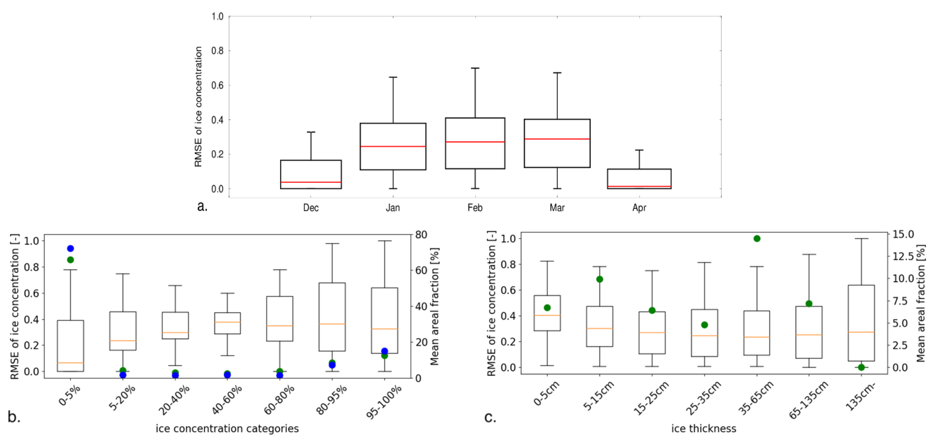
3.1. Erie Ice Skill Statistics

For Lake Erie, the simulation period covers low-, intermediate-, and high-ice years, revealing model performance under a wide array of conditions (Figure 3). In a majority of years, the model successfully follows the lake-wide ice extent as produced by the NIC each year, capturing the initial formation of ice, annual maximum ice, and the ice-off timing, with a few exceptions. The largest divergence between the modeled lake extent and that reported by the NIC occurs during a late-March pulse in 2006 and again in 2017, where the model significantly overpredicts late season ice. In years 2005, 2007, and 2008, and to a lesser extent in 2001, the model also shows a tendency to melt more rapidly in the spring than the NIC. However, in each of these cases, both the model and the NIC showed a decreasing trend in lake-ice leading to the ice-off date. During extreme high- or low-ice years, the model also performs well, where RMSE in the low-ice year of 2012 is 0.01 (Table 2), and in the high-ice years of 2014 and 2015, RMSEs are 0.07 and 0.08, respectively (Table 2).
The overall lake-wide extent RMSE for Lake Erie is 0.12 (Table 2); however most of the error, or difference between the model and the NIC, is found during the periods of rapid ice formation and ice melting, resulting in an “M-shape” in the time series of RMSE (Figure 4). The overall RMSE is higher for spatial concentration (0.17) and higher still for spatial binary (0.23), though the trends between all three RMSE’s are fairly consistent through time (Figure 4). In a few cases, e.g., April–May 2014, the lake-wide error is very low compared to the spatial errors. This indicates that although the model reproduced realistic lake-wide ice extent, the distribution of ice did not agree well with observations, which further motivates the need for spatial skill analyses.
When evaluating spatial concentration RMSE as a function of month (Figure 5a), interestingly, the M-shape pattern that exists in Figure 4 disappears. This is likely because the timing of maximum ice cover shifts from year to year. Thus, in the long-term mean, such patterns are smoothed out, and the larger RMSEs occur during the peak ice months, January through March. In Figure 5b, the model shows the lowest median RMSE for the 0–5% category, indicating that the model performs relatively well over open water or regions with low ice concentration. The data frequency is the highest for 0–5% ice concentration and much lower in the other categories, showing a slight increase toward the higher ice concentration categories. Such distribution is well captured by the model. When RMSEs are evaluated as a function of modeled ice thickness (Figure 5c), the median RMSE is slightly higher at the thinnest ice thickness range (0–5 cm), and then fairly comparable across the other ice thickness categories. The data frequency shows that the modeled ice thickness is the most common for the 35–65 cm range, and least common for ice thicker than 135 cm. Due to the limited availability of observational ice thickness data, no validation is possible at the time of this writing.

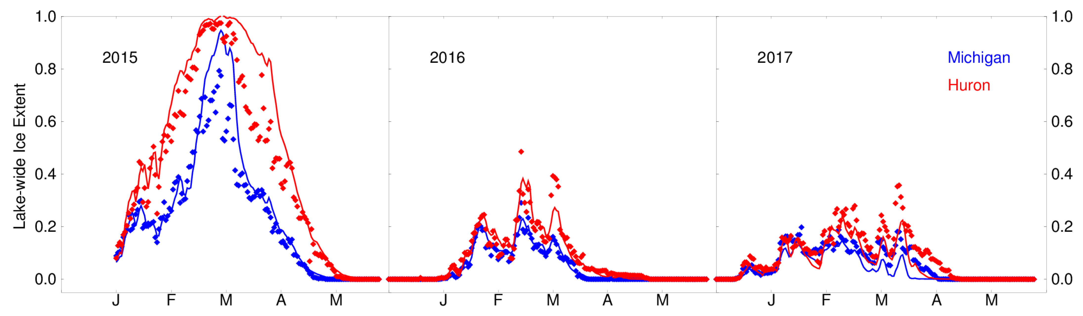
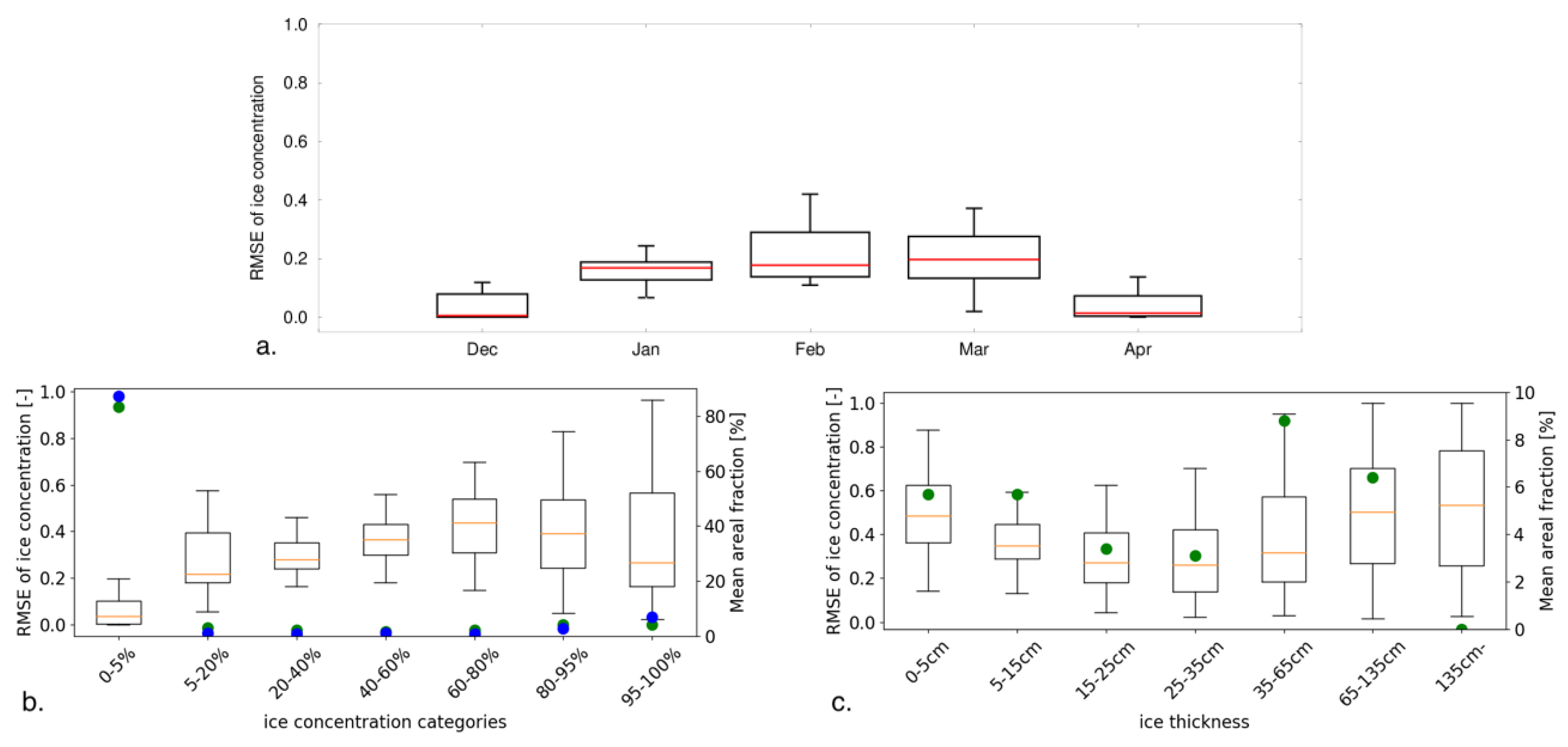
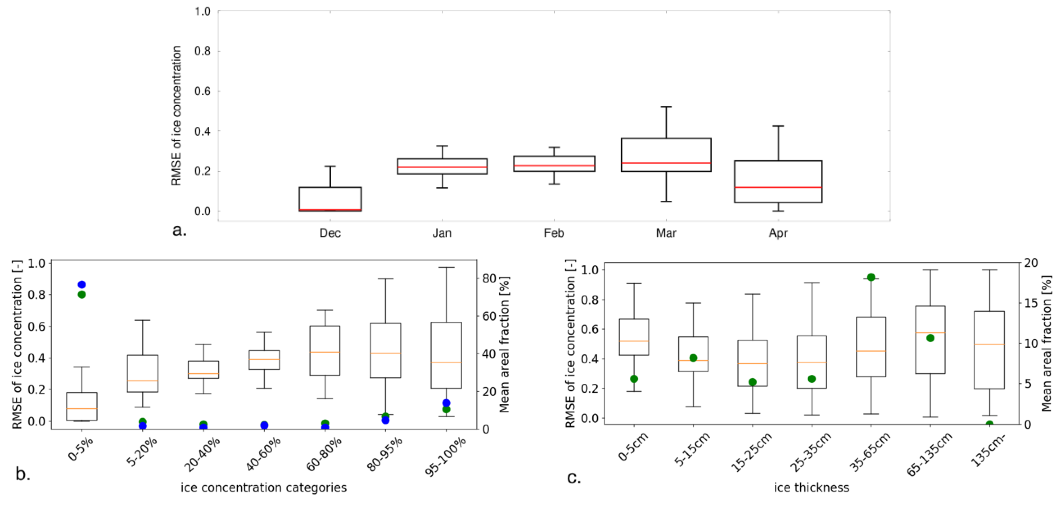
3.2. Michigan-Huron Ice Skill Statistics

For the Lake Michigan-Huron model, the results are similar to those seen for Lake Erie, even with a shorter simulation period. However, unlike Lake Erie, ice formation is primarily constrained to the shallow bays and coastal areas during freezing, peak ice, and melting periods (Figure 2). Time series of ice extent shows a reasonable agreement between simulated and NIC peak ice for all three years (Figure 6). In the heavy-ice year of 2015, the peak ice in Lake Michigan is slightly overpredicted; however, ice melting is captured, resulting in a mean RMSE of 0.09 (Table 2). In Lake Huron, the opposite is true, where peak ice matches well with NIC, but the model experiences a slower decline in ice melting, contrary to the melting trend in Lake Erie, and results in a slightly higher RMSE (0.13, Table 2). In 2016 and 2017, both intermediate- to low-ice years, simulated lake-wide ice extent follows the NIC more closely with the exception of the very end of the 2017 season. Unlike the Lake Erie results, the error time series in Figure 7 does not show the M-shape pattern except for Lake Huron in 2015. This is likely because ice cover is not restricted by the coastlines for Michigan and Huron, except for under conditions with unusually high ice cover (e.g., Huron in 2015).
Overall lake-wide RMSE between the model and NIC are 0.05 for Lake Michigan and 0.07 for Lake Huron, respectively. Similar to Erie, the spatial RMSE is higher for concentration, 0.12 and 0.17 for Michigan and Huron, and higher still for binary with 0.19 and 0.24. The RMSE trends as functions of time, thickness and concentration for Lakes Michigan and Huron (Figure 8 and Figure 9) are also similar to that of Erie. Again, the lowest median RMSE occurs at 0–5% ice concentration, and the median RMSE’s are largest for the thinnest ice (0–5 cm).

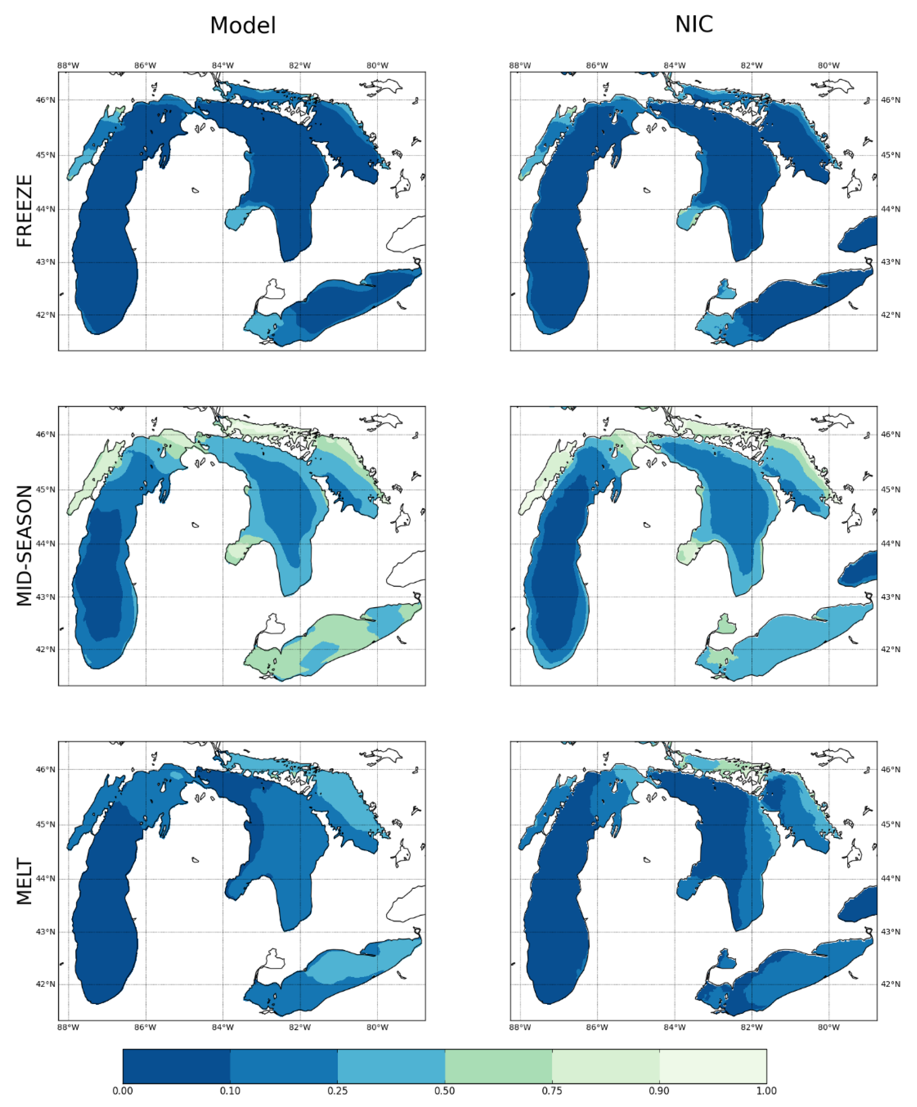
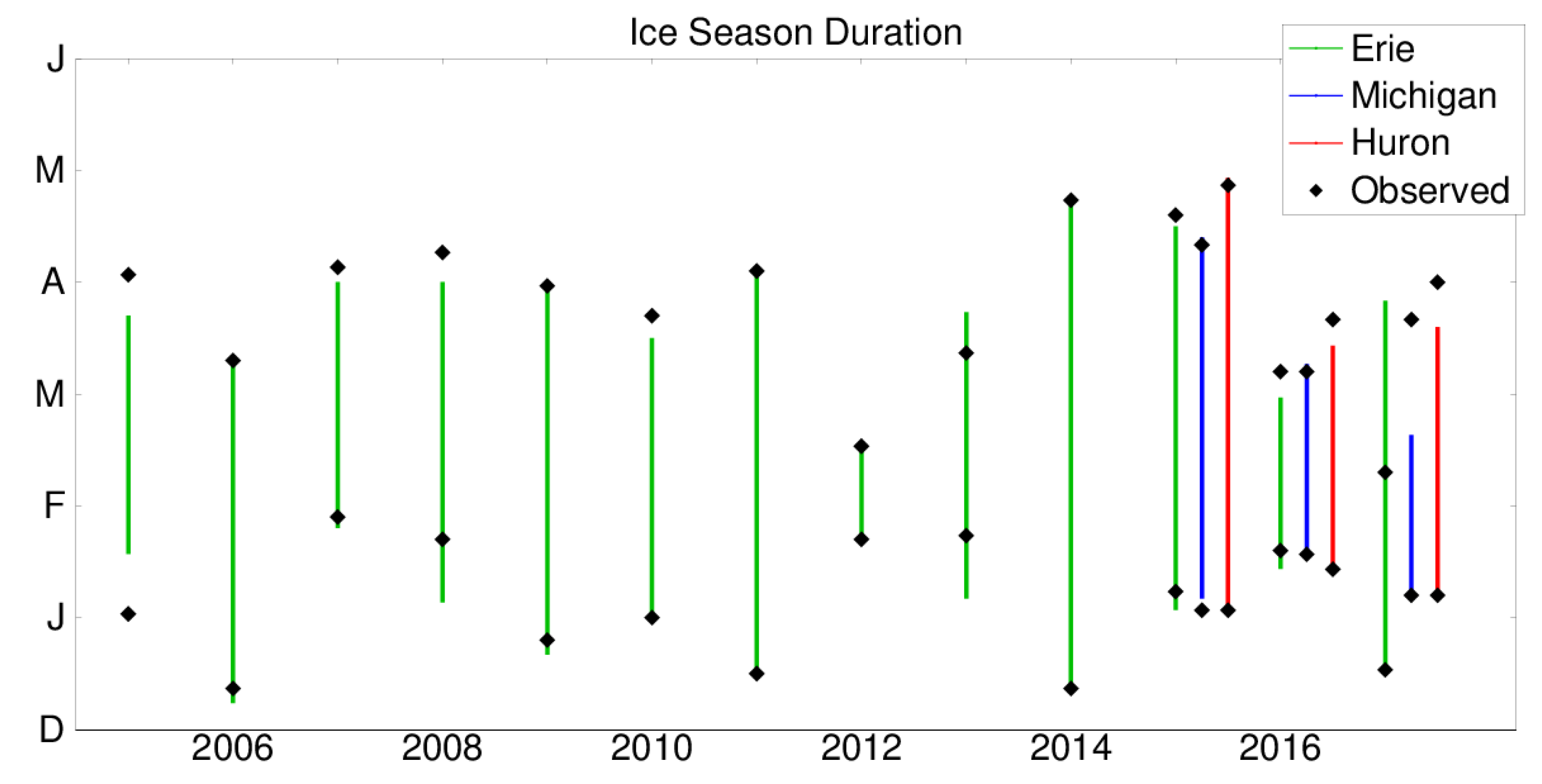
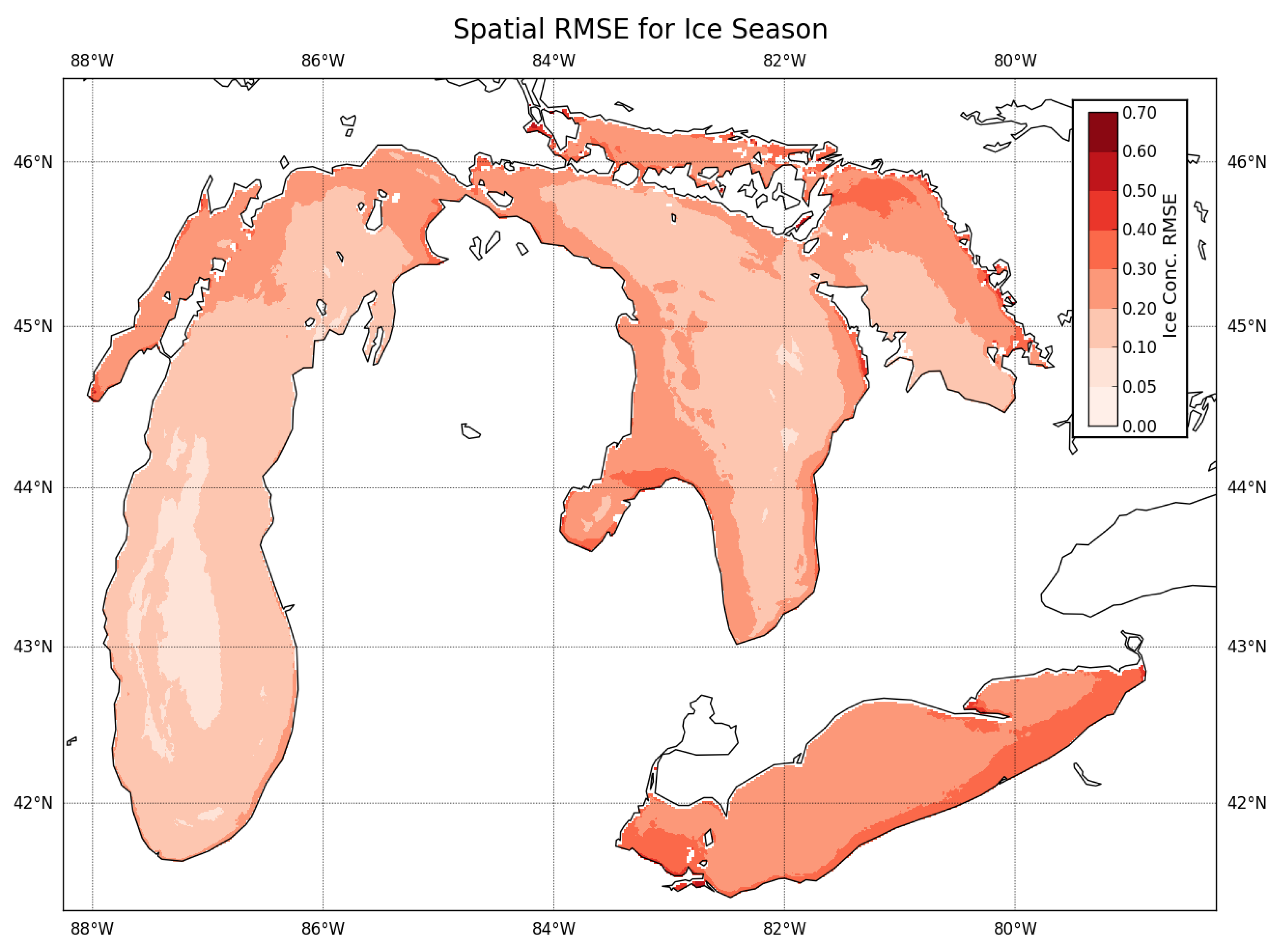
3.3. Ice Duration and Spatial Maps

Based on the lake-wide extent analyzed above, ice on and off dates by the models are compared with the NIC in all simulations years (Figure 10, Table 3). For Erie, 10 of the 13 simulated years show very good agreement with observed ice onset (within 5 days), and 5 of 13 years show extremely good agreement (within 1 day). Erie ice-off dates show a similar trend (9/13 are within 1 week and 5/13 are within 1 day). However, 2005 and 2017 show notably low skill for Erie. In 2017, the ice-on date by the Lake Erie model matched the NIC within one day but the ice-off date was 46 days later than the NIC. The Lake Michigan and Huron model performs well in producing accurate ice-on dates (Lake Michigan: all within 3 days, Lake Huron: all within 1 day), but show varied results in producing ice-off dates. Please note that in 2017, Michigan and Huron’s modeled ice season ended much too soon, despite the opposite being true for Erie.
Extending the analysis of spatial ice extent, time-averaged spatial error maps are shown in Figure 11 for concentration RMSE. Lakes Michigan and Huron tend to show higher error in the shallow, protected coastal regions and less error offshore. This is likely an artifact of the ice formation pattern discussed earlier, as ice rarely extends to the offshore and thus error is inherently lower (see Figure 2). Erie’s spatial error, which is averaged over a much greater simulation period, is nearly homogeneous. The two regions with increased error are the southern portion of the western basin and the southern portion of the eastern basin, likely related to difficulties in simulating ice-initiation and ice-melting in those regions, respectively. Unlike in Lakes Michigan and Huron, the frequent offshore ice formation in Lake Erie, or absence of open-water conditions, does not produce a similar low-error region in the offshore.

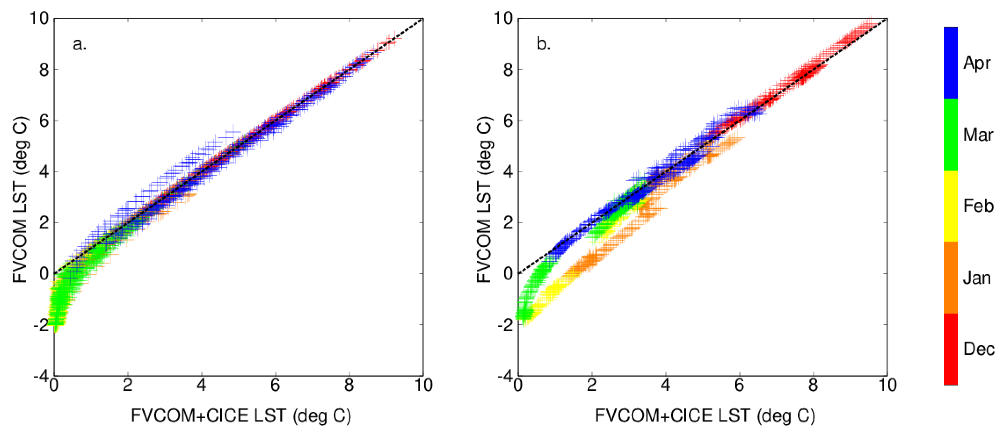
3.4. Water Temperatures

Finally, in terms of the impact on water temperatures, the inclusion of the ice model improves the winter water surface temperatures by eliminating a cold-water bias present in the non-ice simulations (Table 4, Figure 11). This can most likely be attributed to the presence of artificially cooled water in the non-ice simulation, where water temperatures can drop below freezing. Accordingly, the difference between the with and without ice model simulations is evident during the months of January, February, and March (Figure 12). Slight differences between the two simulations are found in April, especially for Lake Erie, which may be improvements made with the ice model simulations where spring warm-up in surface water temperature is realistically delayed by remnant of ice cover later in spring. The RMSE between the model water temperature and GLSEA improves by 0.43 °C for Lake Erie and by 0.21 and 0.26 °C for Michigan and Huron, respectively, when the ice model is activated (Table 4).

4. Discussion

Ice conditions in the Great Lakes result from dynamic processes that yield significant spatio-temporal variability, and most often resemble a continual marginal ice zone that is in constant flux due to atmospheric conditions such as wind speed and direction and air temperature. As such, having updated and accurate information on ice conditions is crucial to safe commercial navigation and United States Coast Guard (USCG) operations. Historically, operational models of the Great Lakes have not included ice conditions as part of the available forecast guidance, and thus decision makers are limited to recent observational-based products such as ice charts produced by the National Ice Center (NIC). In the work presented here, the Los Alamos Sea Ice model (CICE) has been included as part of the next-generational GLOFS and a skill assessment is carried out for Lakes Erie, Michigan, and Huron in regard to modeled ice cover as compared to the NIC.
In general, the FVCOM-CICE model captures the dynamic nature of Great Lakes ice conditions in low-, intermediate-, and high-ice years. The three periods early season freezing or ice formation, mid-season peak ice, and late-season ice melting are reproduced in both Erie and Michigan-Huron. The M-shape of RMSE timeseries indicates relatively high errors in the freezing and melting periods while errors are reduced in the peak period, when model simulations benefit from spatial restrictions by the coastlines. This is evident for Erie in nearly all simulation years and for Huron in 2015. The RMSE timeseries are amplified when spatial distributions of ice are taken into account, indicating limitation of evaluations based on the lake-wide values. The RMSE values for spatial binary ice cover are almost always larger than the corresponding RMSEs for spatial ice concentration. This is rather an artifact of the error calculation with binary ice cover: For example, if modeled ice concentration is 9% at a cell where the NIC has 10%, the differences are only 1% for actual ice concentration but 100% when treated as binary ice cover.
Ultimately, model success must be evaluated based on user requirements for ice concentration accuracy. Interaction with key stakeholders, such as commercial ship captains and the USCG, suggested that although there may be a wide range of requirements depending on conditions or the specific stakeholder, areas of common interest were ice formation and ice-off dates, as well as open versus ice-covered areas. With respect to these measures, the dates of predicted ice initiation and termination were often within 4 days of the NIC (more than half of the Lake Erie simulation years and all of the Lakes Michigan and Huron simulation years). Similarly, the model performed well in predicting areas of open water, often found in Lakes Michigan and Huron, illustrated by the lowest errors found at ice concentration from 0 to 5%. At ice concentrations above 5%, RMSEs were nearly uniform and ranged from 20–40%. In addition, the data frequency is higher at high ice concentrations (>80%), but relatively insignificant at medium ice concentrations (5–80%). These results suggest that stakeholders may find confidence in the model’s ability to predict the binary presence of ice, and thus enable them to plan a shipping route to avoid ice fields. However, if user requirements are established that specifies criteria based on ice concentrations, and/or ice thickness, beyond the presence/absence of ice, more work will be required to evaluate model performance under these guidelines.
Previous work has shown that the next-generation GLOFS, which is based on FVCOM, has performed well for water temperatures in the non-ice period, as well as for currents and water level fluctuations [14,25]. As illustrated, using a coupled FVCOM-CICE model produces an immediate improvement to winter water temperatures, where the ability to form ice when freezing temperatures are reached prevents the unrealistically low water temperatures produced in the existing operational models. This result, in itself, marks an important improvement during the winter season, where often forecast guidance has been limited by unrealistic physical treatment of the lakes (i.e., artificially cooled water).
Discrepancies between modeled and NIC ice concentration may be due to a multitude of reasons. In terms of ice dynamics, some processes that are potentially important for nearshore ice physics are currently not taken into account, such as land-fast ice and ice-wave interaction. Land-fast ice may provide a stable ice zone along the shore resistant to wind disturbance. Surface waves may break ice cover into smaller pieces that are more sensitive to heat fluxes from air and water due to increased contact surface. In terms of ice thermodynamics, inclusion of realistic snow cover on top of the ice would be an important step to the future improvement as it influences calculations of ice albedo and thermal conductivity of the snow/ice medium. Another possible cause for discrepancy could be related to the uncertainty in the meteorological forcing. Previous work has shown that as much as 70% of ice cover variability in the Great Lakes can be explained by surface air temperature alone [45]. As such, the model will show significant sensitivity to the surface air temperature prescribed in the meteorological forcing.
Overall, the addition of an ice model to the existing operational hydrodynamic models can make significant improvements to forecast guidance and support stakeholder needs in navigation, hydropower, recreation, and spill response, as well as enables lake coupling with climate forecast models. As such, this work serves as the precursor to the upgrade of the Great Lakes Operational Forecast System (GLOFS) and to the first-ever operational ice forecast guidance in the Great Lakes within NOAA. As user requirements become better defined, additional skill assessment can guide avenues for model improvement and refinement.

Author Contributions

The paper was conceived of and written by E.A., A.F., and J.K. E.A., A.F., and J.K. carried out the model simulations and post-processing of results. The upgrade of GLOFS was conceived of and is being carried out by E.A., P.C., J.G.W.K., and G.L. The CICE model was adapted to the Great Lakes by A.F. and J.W. Model skill assessment was conceived of by J.G.W.K., Y.C., A.F., and E.A., and carried out by A.F. and J.K.

Funding

This research was carried out with support of the National Oceanic and Atmospheric Administration (NOAA) Great Lakes Environmental Research Laboratory (GLERL) and National Ocean Service (NOS), and the NOAA Research Acceleration Transition Program (RTAP).

Acknowledgments

The authors would like to acknowledge Changshen Chen from the University of Massachusetts Dartmouth for model support, as well as the United States Coast Guard (USCG) and representatives from the Great Lakes shipping community for support and engagement in defining user requirements. This is GLERL contribution number 1899.

Conflicts of Interest

The authors declare no conflicts of interest.

References

  1. Assel, R.; Cronk, K.; Norton, D. Recent trends in Laurentian Great Lakes ice cover. Clim. Chang. 2003, 57, 185–204. [Google Scholar] [CrossRef]
  2. Assel, R.A. A Computerized Ice Concentration Data Base for the Great Lakes; NOAA GLERL: Ann Arbor, MI, USA, 1983. [Google Scholar]
  3. Wang, J.; Kessler, J.; Hang, F.; Hu, H.; Clites, A.; Chu, P. Great Lakes Ice Climatology Update of Winters 2012–2017: Seasonal Cycle, Interannual Variability, Decadal Variability, and Trend for the Period; NOAA GLERL: Ann Arbor, MI, USA, 2017; pp. 1–14. [Google Scholar]
  4. Wang, J.; Bai, X.; Hu, H.; Clites, A.; Colton, M.; Lofgren, B. Temporal and spatial variability of Great Lakes ice cover, 1973–2010. J. Clim. 2012, 25, 1318–1329. [Google Scholar] [CrossRef]
  5. Wang, J.; Hu, H.; Schwab, D.; Leshkevich, G.; Beletsky, D.; Hawley, N.; Clites, A. Development of the Great Lakes Ice-circulation Model (GLIM): Application to Lake Erie in 2003–2004. J. Gt. Lakes Res. 2010, 36, 425–436. [Google Scholar] [CrossRef]
  6. Rondy, D.R. Great Lakes Ice Cover, Great Lakes Basin Framework Study; Appendix 4; Great Lakes Basin Commission: Ann Arbor, MI, USA, 1976. [Google Scholar]
  7. Bolsenga, S.J. A Review of Great Lakes Ice Research. J. Gt. Lakes Res. 1992, 18, 169–189. [Google Scholar] [CrossRef]
  8. Hawley, N.; Beletsky, D.; Wang, J. Ice thickness measurements in Lake Erie during the winter of 2010–2011. J. Gt. Lakes Res. 2018, 44, 388–397. [Google Scholar] [CrossRef]
  9. Wright, D.M.; Posselt, D.J.; Steiner, A.L. Sensitivity of Lake-Effect Snowfall to Lake Ice Cover and Temperature in the Great Lakes Region. Mon. Weather Rev. 2013, 141, 670. [Google Scholar] [CrossRef]
  10. Assel, R.A.; Quinn, F.H.; Sellinger, C.E. Hydroclimatic Factors of the Recent Record Drop in Laurentian Great Lakes Water Levels. BAMS 2004, 1144–1148. [Google Scholar] [CrossRef]
  11. Xiao, C.; Lofgren, B.M.; Wang, J. WRF-Based assessment of the Great Lakes’ impact on cold season synoptic cyclones. Atmos. Res. 2018, 214, 189–203. [Google Scholar] [CrossRef]
  12. Vanderploeg, H.A.; Bolsenga, S.J.; Fahnenstiel, G.L.; Liebeg, J.R.; Gradner, W. Plankton ecology in an ice covered bay of Lake Michigan: Utilization of a winter phytoplankton bloom by reproduccing copepods. Hydrobiologia 1992, 243–244, 175–183. [Google Scholar] [CrossRef]
  13. Martin Associates. Lawrence Region Economic Impacts of Maritime Shipping in the Great Lakes-St.Lawrence Region; US Department of Transportation: Washington, DC, USA, 2018 July.
  14. Kelley, J.G.W.; Chen, Y.; Anderson, E.J.; Lang, G.A.; Xu, J. Upgrade of NOS Lake Erie Operational Forecast System (LEOFS) to FVCOM: Model Development and Hindcast Skill Assessment; NOS CS 40, NOAA; NOAA Technical Memorandum: Silver Spring, MD, USA, 2018. [Google Scholar]
  15. Kelley, J.G.W.; Chu, P.; Zhang, A.; Lang, G.A.; Schwab, D.J. Skill Assessment of NOS Lake Michigan Operational Forecast System (LMOFS); NOS CS 8, NOAA; NOAA Technical Memorandum: Silver Spring, MD, USA, 2007. [Google Scholar]
  16. Kelley, J.G.W.; Zhang, A.; Chu, P.; Lang, G.A. Skill Assessment of NOS Lake Huron Operational Forecast System (LHOFS); NOS CS 23, NOAA; NOAA Technical Memorandum: Silver Spring, MD, USA, 2010. [Google Scholar]
  17. Mellor, G.L. Users Guide for Ocean Model. Ocean Model. 2004, 8544, 0710. [Google Scholar]
  18. Schwab, D.J.; Bedford, K.W. Initial Implementation of the Great Lakes Forecasting System: A Real-Time System for Predicting Lake Circulation and Thermal Structure. Water Qual. Res. J. 1994, 29, 203–220. [Google Scholar] [CrossRef]
  19. Chen, C.; Beardsley, R.C.; Cowles, G. An unstructured grid, finite volume coastal ocean model (FVCOM) system. Oceanography 2006, 19, 78–89. [Google Scholar] [CrossRef]
  20. Hunke, E.C.; Lipscomb, W.H.; Turner, A.K.; Jeffery, N.; Elliott, S. CICE: The Los Alamos Sea Ice Model Documentation and Software User’s Manual LA-CC-06-012; Los Alamos National Laboratory: Santa Fe, NM, USA, 2015; Volume 115.
  21. Xue, P.; Pal, J.S.; Ye, X.; Lenters, J.D.; Huang, C.; Chu, P.Y. Improving the simulation of large lakes in regional climate modeling: Two-way lake-atmosphere coupling with a 3D hydrodynamic model of the great lakes. J. Clim. 2017, 30, 1605–1627. [Google Scholar] [CrossRef]
  22. Anderson, E.J.; Schwab, D.J.; Lang, G.A. Real-Time Hydraulic and Hydrodynamic Model of the St. Clair River, Lake St. Clair, Detroit River System. J. Hydraul. Eng. 2010, 136, 507–518. [Google Scholar] [CrossRef]
  23. Anderson, E.J.; Bechle, A.J.; Wu, C.H.; Schwab, D.J.; Mann, G.E.; Lombardy, K.A. Reconstruction of a meteotsunami in Lake Erie on 27 May 2012; Roles of atmospheric conditions on hydrodynamic response in enclosed basins. J. Geophys. Res. 2015, 120, 1–16. [Google Scholar] [CrossRef]
  24. Anderson, E.J.; Schwab, D.J. Meteorological influence on summertime baroclinic exchange in the Straits of Mackinac. J. Geophys. Res. Oceans 2017, 122. [Google Scholar] [CrossRef]
  25. Anderson, E.J.; Schwab, D.J. Predicting the oscillating bi-directional exchange flow in the Straits of Mackinac. J. Gt. Lakes Res. 2013, 39, 663–671. [Google Scholar] [CrossRef]
  26. Bai, X.; Wang, J.; Schwab, D.J.; Yang, Y.; Luo, L.; Leshkevich, G.A.; Songzhi, L. Modeling 1993–2008 climatology of seasonal general circulation and thermal structure in the Great Lakes using FVCOM. Ocean Mod. 2013, 64, 40–63. [Google Scholar] [CrossRef]
  27. Luo, L.; Wang, J.; Schwab, D.J.; Vanderploeg, H.A.; Leshkevich, G.A.; Bai, X.; Hu, H.; Wang, D. Simulating the 1998 spring bloom in Lake Michigan using a coupled physical-biological model. J. Geophys. Res. 2012, 117, 14. [Google Scholar] [CrossRef]
  28. Smagorinsky, J. General Circulation Experiments with the Primitive Equations. Mon. Weather Rev. 1963, 91, 99–164. [Google Scholar] [CrossRef]
  29. Mellor, G.L.; Yamada, T. Development of a turbulent closure model for geophysical fluid problems. Rev. Geophys. 1982, 20, 851–875. [Google Scholar] [CrossRef]
  30. Large, W.G.; Pond, S. Open Ocean momentum flux measurements in moderate to strong winds. J. Phys. Oceanogr. 1981, 11, 324–336. [Google Scholar] [CrossRef]
  31. Fairall, C.W.; Bradley, E.F.; Rogers, D.P.; Edson, J.B.; Young, G.S. Bulk parameterization of air-sea fluxes for Tropical Ocean-Global Atmosphere Coupled-Ocean Atmosohere Response Experiment. J. Geophys. Res. 1996, 101, 3747–3764. [Google Scholar] [CrossRef]
  32. Fairall, C.W.; Bradley, E.F.; Godfrey, J.S.; Wick, G.A.; Edson, J.B.; Young, G.S. Cool-skin and warm-layer effects on sea surface temperature. J. Geophys. Res. 1996, 101, 1295–1308. [Google Scholar] [CrossRef]
  33. Fairall, C.W.; Bradley, E.F.; Hare, J.E.; Grachev, A.A.; Edson, J.B. Bulk parameterization of air-sea fluxes: Updates and verification for the COARE algorithm. J. Clim. 2003, 16, 571–591. [Google Scholar] [CrossRef]
  34. Liu, P.C.; Schwab, D.J. A comparison of methods for estimating u*, from given uz and air-sea temperature differences. J. Geophys. Res. 1987, 92, 6488–6494. [Google Scholar] [CrossRef]
  35. Gao, G.; Chen, C.; Qi, J.; Beardsley, R.C. An unstructured-grid, finite-volume sea ice model: Development, validation, and application. J. Geophys. Res. Oceans 2011, 116, 1–15. [Google Scholar] [CrossRef]
  36. Hunke, E.C.; Dukowicz, J.K. An Elastic–Viscous–Plastic Model for Sea Ice Dynamics. J. Phys. Oceanogr. 1997, 27, 1849–1867. [Google Scholar] [CrossRef] [Green Version]
  37. Thorndike, A.S.; Rothrock, D.A.; Maykut, G.A.; Colony, R. The Thickness Distribution of Sea Ice. J. Geophys. Res. 1975, 80, 4501. [Google Scholar] [CrossRef]
  38. Briegleb, B.; Bitz, C.; Hunke, E.; Lipscomb, W.; Schramm, J. Description of the Community Climate System Model Version 2: Sea Ice Model; UCAR: Boulder, CO, USA, 2002. [Google Scholar]
  39. Proshutinsky, A.; Steele, M.; Zhang, J.; Holloway, G.; Steiner, N.; Häkkinen, S.; Holland, D.M.; Gerdes, R.; Koeberle, C.; Karcher, M.; et al. The Arctic Ocean Model Intercomparison Project (AOMIP). EOS Trans. Am. Geophys. Union 2001, 82, 637–644. [Google Scholar] [CrossRef]
  40. Maykut, G.A.; McPhee, M.G. Solar Heating of the Arctic Mixed Layer. J. Geophys. Res. Oceans 1995, 100, 24691–24703. [Google Scholar] [CrossRef]
  41. Schwab, D.J.; Leshkevich, G.A.; Muhr, G.C. Automated mapping of surface water temperature in the Great Lakes. J. Gt. Lakes Res. 1999, 25, 468–481. [Google Scholar] [CrossRef]
  42. Beletsky, D.; Schwab, D.J.; Roebber, P.J.; McCormick, M.J.; Miller, G.S.; Saylor, J.H. Modeling wind-driven circulation during the March 1998 sediment resuspension event in Lake Michigan. J. Geophys. Res. Oceans 2003, 108. [Google Scholar] [CrossRef] [Green Version]
  43. Benjamin, S.G.; Weygandt, S.S.; Brown, J.M.; Hu, M.; Alexander, C.R.; Smirnova, T.G.; Olson, J.B.; James, E.P.; Dowell, D.C.; Grell, G.A.; et al. A North American hourly assimilation and model forecast cycle: The rapid refresh. Mon. Weather Rev. 2016, 144, 1669–1694. [Google Scholar] [CrossRef]
  44. U.S. National Ice Center: Naval Ice Center. Available online: www.natice.noaa.gov/products/great_lakes.html (accessed on 1 July 2018).
  45. Titze, D. Characteristics, Influence, and Sensitivity of Ice Cover in the Great Lakes. Ph.D. Thesis, University of Minnesota, Minneapolis, MN, USA, November 2016. [Google Scholar]
Figure 1. The Great Lakes domain, including Lakes Erie, Michigan, and Huron.
Jmse 06 00123 g001
Figure 2. Spatial pattern of ice concentration (0–1) for freezing (1 December–15 January), mid-season (16 January–15 March), and melting (15 March–1 May) seasons. Averaging is performed for each season from 2015–2017. Left column shows the model results from LEOFS and LMHOFS, and right column shows the NIC analysis.
Jmse 06 00123 g002
Figure 3. Simulated lake-wide average ice extent for Lake Erie (green line) and the ice extent from the NIC (black dots).
Jmse 06 00123 g003
Figure 4. Time series of ice simulation errors between the Lake Erie model and the NIC based on the three methods: Pixel-to-pixel RMSE based on ice concentration (cyan), pixel-to-pixel RMSE based on binary ice cover (orange), and lake-wide absolute error (black). Please note that lake-wide absolute error shows only the magnitude of error (i.e., does not show the sign of model bias).
Jmse 06 00123 g004
Figure 5. Ranges of spatial concentration RMSE as functions of (a) months, (b) observed ice concentration, and (c) modeled ice thickness for the LEOFS 2005-2017 simulation results. A box extends from the lower and upper 25% of the RMSEs. A horizontal line within each box denotes the median value. The whiskers show the range of RMSE, extending from the box toward farthest data points within the interquartile range (i.e., length of the box) from the upper and lower bounds of the box. In (b,c), solid circles show mean areal fractions for observation (blue) and model (green), representing data frequency for each category. For (c), open water cells are excluded.
Jmse 06 00123 g005
Figure 6. Lake-wide average ice extent for Lake Michigan (blue) and Lake Huron (red). The model ice extent (solid lines) is compared to the NIC (diamonds).
Jmse 06 00123 g006
Figure 7. Time series of ice simulation errors between the Lake Michigan-Huron model and the NIC based on the three methods for (top) Lake Michigan and (bottom) Lake Huron: Pixel-to-pixel RMSE based on ice concentration (cyan), pixel-to-pixel RMSE based on binary ice cover (orange), and lake-wide absolute error (black). Please note that lake-wide absolute error shows only the magnitude of error (i.e., does not show the sign of model bias).
Jmse 06 00123 g007
Figure 8. Ranges of spatial concentration RMSE as functions of month (a), ice concentration (b) and ice thickness (c) for Lake Michigan from the LMHOFS 2015–2017 simulation results. See the caption of Figure 5 for the explanation of the box, whiskers, and solid circles. For (c), open water cells are excluded.
Jmse 06 00123 g008
Figure 9. Ranges of spatial concentration RMSE as functions of month (a), ice concentration (b) and ice thickness (c) for Lake Huron from the LMHOFS 2015–2017 simulation results. See the caption of Figure 5 for the explanation of the box, whiskers, and solid circles. For (c), open water cells are excluded.
Jmse 06 00123 g009
Figure 10. Modeled vs observed ice season duration for all simulated years. The duration is defined as the period of time between ice onset (first day lake-wide extent exceeds 10%) and ice-off (last day extent exceeds 10%). The y-axis shows the length and timing of the ice season by month.
Jmse 06 00123 g010
Figure 11. Spatial distribution of ice concentration RMSE averaged throughout the entire ice season for all simulated years.
Jmse 06 00123 g011
Figure 12. Lake surface temperature (LST) for Lake Erie (left) and Lake Michigan-Huron (right) for simulations of FVCOM with and without CICE during the winter months.
Jmse 06 00123 g012
Table 1. Average annual maximum ice cover for the period 1973–2018.
Lake ObservationsSuperiorMichiganHuronErieOntarioBasin
Average Max. ice cover (%)60.9139.6464.6082.1929.7754.28
Table 2. Seasonal mean RMSEs [0–1] of simulated lake-wide ice area, ice concentration at pixels, and binary ice cover at pixels. The lake-wide RMSEs are normalized by an area of each lake. The seasonal means are calculated from 1 December in the previous year to 31 May.
YearErieMichiganHuron
lake widespatiallake widespatiallake widespatial
concentrationbinary concentrationbinary concentrationbinary
20050.17 10.21 10.25 1
20060.170.150.24
20070.080.130.17
20080.190.220.26
20090.100.180.25
20100.120.190.26
20110.110.210.25
20120.010.030.06
20130.130.160.23
20140.070.180.23
20150.080.150.180.09 10.20 10.31 10.13 10.26 10.34 1
20160.090.100.170.010.070.110.030.120.18
20170.280.260.380.040.100.150.050.140.21
mean0.120.170.230.050.120.190.070.170.24
1 Averaging period for the initial year (2005 for LEOFS and 2015 for LMHOFS) is from 1 January to 31 May.
Table 3. Ice season length (in days) as defined in Figure 10.
YearErieMichiganHuron
NICModelNICModelNICModel
20059164
20068892
20076766
20087786
200995100
20108176
2011108107
20122524
20134977
2014131131
20151011039897114115
2016484649506759
2017539874428471
Table 4. Surface water temperature RMSE (°C) between model simulations and observed temperatures from satellite-derived lake surface temperature from the GLSEA during winter months (1 December–30 April).
Satellite-Derived TemperatureFVCOM-CICEFVCOM (No-Ice)
Lake Erie GLSEA0.691.12
Lake Michigan GLSEA0.660.87
Lake Huron GLSEA0.680.94

