A Multi-Objective Optimization Method for Maritime Search and Rescue Resource Allocation: An Application to the South China Sea

Abstract

To effectively address the increase in maritime accidents and the challenges posed by the trend toward larger ships for maritime safety, it is crucial to rationally allocate the limited maritime search and rescue (MSAR) resources and enhance accident response capabilities. We present a comprehensive method for allocating MSAR resources, aiming to improve the overall efficiency of MSAR operations. First, we use long short-term memory to predict the number of future accidents and employ the K-medoids algorithm to identify the accident black spots in the studied area. Next, we analyze the multi-constraint conditions in the MSAR resource allocation process. A multi-objective integer programming model is constructed to minimize the response time and allocation cost. Finally, we use the non-dominated sorting genetic algorithm II (DNSGA-II) with Deb’s rules to solve the model, and we propose a multi-attribute decision optimization-based method for MSAR resource allocation. We found that the DNSGA-II exhibits better convergence and generates higher-quality solutions compared to the NSGA-II, particle swarm optimization (PSO), and enhanced particle swarm optimization (EPSO) algorithms. Compared with the existing MSAR resource emergency response system, the optimized scheme reduces the response time and allocation cost by $11.32\%$ and $6.15\%$, respectively. The proposed method can offer decision makers new insights when formulating MSAR resource allocation plans.

1. Introduction

In the process of global economic integration, the number and scale of transnational trade are continuously increasing. Due to maritime transportation’s advantages of higher capacity, lower cost, extensive coverage, and efficiency, the international shipping industry undertakes about 90% of international trade tasks [1]. Even under the negative impacts of events such as the COVID-19 pandemic, the Suez Canal blockage, and the Russia–Ukraine conflict, global maritime logistics still maintain a relatively high level of productivity. With the rapid development of marine economic activities, the maritime traffic density and the number of ships entering and leaving ports have increased significantly [2]. Furthermore, the increase in aquaculture activities and fishing vessels, combined with the absence of distinct routes or markers between islands, has heightened the probability of maritime accidents. Moreover, influenced by the increasing scale and carrying capacity of ships, the magnitude of accidents has reached unprecedented levels, causing severe damage to both the socioeconomic and ecological environments [3]. For instance, the collision between the “Sanchi” tanker and the “CF Crystal” bulk carrier in 2018 resulted in the leakage of 111,300 metric tons of condensate oil and nearly 2000 tons of fuel oil. According to estimates, the recovery of the marine ecological environment from the damage caused by the accident is expected to take at least 60 years [4].

Rapid and effective emergency coordination and response can reduce casualties and economic losses, protect the environment, and ensure the safety of maritime navigation [5]. After a maritime accident, decision makers should formulate corresponding emergency measures scientifically and flexibly according to the actual situation to ensure that sufficient maritime search and rescue (MSAR) resources can quickly reach the accident site. In addition, the rational allocation of MSAR resources can significantly enhance overall rescue efficiency, minimize potential losses caused by accidents, and control the occurrence of secondary disasters. Due to variable marine climate conditions and unclear disposal information, the extent of disasters cannot be accurately estimated. Therefore, the allocation of MSAR resources needs to consider various factors such as the location of rescue bases, the type of resources, the type of ships and aircraft, and the characteristics of the sea area.

The existing research on MSAR can be roughly divided into two categories: passive response and proactive defense. The former focuses on effectively addressing and responding to accidents to maximize the accuracy and efficiency of MSAR. The main research directions include the trajectory prediction of objects in distress, the scheduling of MSAR resources, and search coverage planning for rescue equipment. The latter emphasizes taking measures before accidents occur to enhance the overall effectiveness of MSAR efforts. The main research directions include the prediction of demand for MSAR resources and the allocation of MSAR resources.

The accurate track prediction of objects in distress is the basis of MSAR operations. Analyzing the drift patterns of maritime targets under the influence of the background field and establishing a fitting equation for target motion is the essence of target drift prediction [6]. Due to the influence of environmental factors such as wind, ocean currents, and waves, objects in distress at sea exhibit significant time-varying characteristics. Therefore, in the event of a maritime accident, it is essential to accurately predict the drift trajectory and current location of the distressed target as a first step. However, due to the complex and changeable marine meteorological environment, it is challenging to predict the precise location of the object in distress. Usually, only the approximate area where the target may be located can be determined [7], allowing focused search efforts in that region.

After identifying the critical search areas, the MSAR resources should arrive at the location of distress as quickly as possible. The scheduling of MSAR resources integrates the constraints of time variability, demand uncertainty, capacity limitation, and transportation capacity limitation of rescue equipment, which can be seen as a complex nonlinear decision problem. These constraints often result in low rescue response efficiency and high costs. To address these challenges, researchers have developed various search and planning decision support systems [8]. However, most of the existing studies have adapted methods and approaches from onshore emergency resource scheduling, with limited consideration for the unique characteristics of maritime accidents. This limitation makes it difficult to ensure the scientific validity and efficiency of MSAR resource scheduling [9].

After MSAR equipment arrives at the accident area, excessive search times can result in individuals going missing or losing their lives. Therefore, a path should be planned for MSAR equipment to cover the search area quickly. The search coverage problem has been proven to be an NP-complete problem [10], and it is often solved using the random coverage algorithm [11]. People in distress at sea have a shorter survival time than those on land, and the golden rescue time is fleeting. In addition, the uncertainty of the location of objects in distress, the larger search area, and the variable marine environment make the search path planning at sea more challenging.

Passive responses after maritime accidents can enhance response efficiency and MSAR accuracy to a certain extent, thereby reducing losses. However, when accidents occur in remote seas or as multiple frequent accidents, rescue efficiency may still be severely limited if the MSAR resources at the rescue base are insufficient. Therefore, it becomes especially important to allocate sufficient MSAR resources for ships and personnel in distress before maritime accidents occur [12,13]. When allocating MSAR resources, it is vital to find the right balance between response efficiency and cost considerations. Insufficient MSAR resources at the base nearest the accident area can lead to significant delays and decreased response efficiency when coordinating and deploying resources from more distant bases. Conversely, if excessive MSAR resources are allocated to the base, costs may also increase, affecting the overall economic benefits [14].

Therefore, we conducted interviews with renowned maritime safety experts and several officials from the South China Sea Rescue Bureau. These experts shared their personal experiences in maritime search and rescue, which is helpful for us in enhancing the understanding of the actual requirements for MSAR allocations and developing a comprehensive method that appropriately addresses these needs. The interviewees pointed out that the current allocation of MSAR resources often relies on subjective experience. This subjective reliance can lead to decreased rescue efficiency, hindering timely and effective responses to maritime accidents. Due to the unique and complex nature of maritime accidents, a more scientific and systematic approach is necessary for MSAR resource allocation. Drawing upon an extensive array of the relevant literature, accident reports, and expert opinions, we recognized the necessity and urgency of developing a novel MSAR resource allocation method. This method encompasses predicting MSAR resource needs, allocating models, and employing solution algorithms. Moreover, it can seek to obtain a balanced solution that optimizes both response times and resource allocation costs, thus enhancing the overall efficiency of MSAR.

The remainder of this paper is organized as follows. Section 2 provides a review of MSAR resources to reveal the research gaps in the field. Section 3 discusses the MSAR resource allocation problem, presents the optimization model for MSAR resource allocation, and outlines the specific process of solving the model. In Section 4, we apply our method to the Chinese waters of the South China Sea to validate its rationality. Some conclusions are drawn in Section 5.

2. Literature Review

Currently, the research field of search and rescue (SAR) resource allocation mainly focuses on urban emergency responses after natural disasters, which encompasses the selection of rescue facilities (e.g., hospitals, fire stations, emergency shelters, etc.) and the allocation of emergency resources in existing warehouses and shelters explicitly [15,16,17]. In contrast, research on the allocation of MSAR resources is limited. Hence, to enhance the overall effectiveness of MSAR, it is essential to design a proactive prevention strategy that focuses on the rational allocation of various types of MSAR resources before accidents.

A reasonable MSAR resource allocation plan consists of three steps: first, predicting the required MSAR resources; second, establishing an MSAR resource allocation model based on the actual situation; and finally, combining the predicted demand with the model to formulate a rational resource allocation plan.

The existing research on predicting demand for SAR resources primarily concentrates on land-based emergencies, typically employing methods such as time-series theory [18], case-based reasoning [19,20], and neural networks [21]. Methods based on time-series theory, including autoregressive moving averages, exponential smoothing, and independent and identically distributed methods, have been widely used in forecasting emergency demand. However, these methods often perform poorly when dealing with uncertainty in multiple demands [22]. The case-based reasoning method makes predictions based on the similarity between existing cases. This approach is primarily suitable for addressing straightforward scenarios and exhibits suboptimal performance when applied to intricate demand-forecasting challenges. In contrast, neural networks can learn the temporal and spatial correlations in data, excelling in handling complex problems with incomplete information and high uncertainty. Due to the distinctions between sea and land environments, current methods for predicting MSAR resources mainly depend on analyzing historical cases in conjunction with expert assessments. However, this type of method often suffers from significant subjectivity and lacks scientific rigor. Thus, we use neural networks to forecast the number of accidents and determine the types and quantities of MSAR resources.

In addition to the prediction of MSAR resource demand, the allocation model of MSAR resources should be established when making the allocation scheme. Typically, there are two types of available rescue equipment: rescue ships and rescue aircraft. Rescue ships are the primary tool for MSAR, and they have the advantages of extended endurance, high passenger capacity, and comprehensive equipment, albeit at lower speed. Rescue aircraft have the advantages of fast flight speed and a wide search area, but their endurance is relatively short. In terms of rescue equipment, the existing research on allocating MSAR resources can be divided into three categories: (1) rescue ships, (2) rescue aircraft, and (3) a combination of ships and aircraft.

In the MSAR resource allocation research that only focuses on rescue ships, the most representative study is by the authors of [23]. To increase ship utilization and reduce fleet operation costs, they developed a multi-objective integer programming model considering scarce types of rescue ships. This model can provide the U.S. Coast Guard with ship configuration plans for different seasons. Additionally, it does not consider the factor of response efficiency, which is a key concern for many MSAR organizations. The authors of [24] then took the response time into account and developed an event-based, multiple-ship allocation model based on the maritime conditions in the Aegean Sea. The authors of [25] established a configuration model considering four types of ships with different capabilities based on criteria such as the coverage of critical rescue areas and average response time to multiple accident locations. Subsequently, the authors of [26] conducted further research on the allocation of rescue ships, considering the workload balance between ships and the recruitment of new ships for future rescue efforts. The authors of [27] developed an optimization model considering emergency resources and ships with different capabilities. Based on the distribution characteristics of accidents, this model was designed to balance the cost of configuration and the safety of a ship in distress. The model was applied in China’s Bohai Sea to verify its scientific validity.

Some research studies only consider rescue aircraft in the allocation of resources at sea. To reduce operating costs, the authors of [28] established an aircraft configuration optimization model considering the capacity and endurance of the airport. They used a combination method of optimization and simulation to solve the model. The authors of [29], aiming to achieve a rapid response to accidents, established an integer linear programming model. They used a rule-based algorithm to solve the model and obtain multiple configuration plans. The authors of [30] developed four single-objective binary integer programming models, each aiming to optimize a different aspect, including maximizing the coverage of search areas, minimizing the response time, minimizing the total aircraft working time, and minimizing overall rescue costs. This method was applied in scenarios involving aircraft participation in open-sea rescue.

Rescue ships and rescue aircraft have their advantages and disadvantages. Effectively coordinating the two limited resources is crucial for enhancing the overall efficiency of MSAR. Currently, there is relatively limited research on the combination of ships and aircraft. The authors of [31] established a multi-objective integer nonlinear programming model with the optimization objectives of improving equipment utilization and the survival rate of castaway individuals in remote maritime emergency responses. They applied the model in the Bohai Sea to validate its effectiveness. The author of [5] analyzed historical accident data and discovered that the frequencies of different types of accidents are correlated with the seasons. Subsequently, he used kernel density estimation to calculate the probability of future accidents occurring in each region of the study area. Then, he established a model for the allocation of rescue ships and aircraft under demand uncertainty based on the probabilities. To enhance the efficiency of long-range MSAR responses, the authors of [32] considered the availability of surrounding islands. They established a nonlinear optimization model and obtained configuration plans by solving the model with an improved particle swarm algorithm. The authors of [33] used a geospatial technique and a fuzzy analytic hierarchy process approach to obtain risk values for the responsibility zones of various rescue bases. Based on the obtained risk values, the game theory was employed for reallocating rescue ships and aircraft.

To facilitate the literature analysis, we present a brief literature summary in

Table 1. Overview of studies on MSAR resource allocation related to this paper.

Reference	Main Objectives			Problem Description					Model Features
	Time	Cost	Others	SAR Ships	SAR Aircraft	Emergency Resources	Rescue Bases	Black Spots	Solution Method	Multi-Obj. Approach
[23]		✓	✓	M			M		EXC	FLP
[24]	✓	✓	✓	M			M	M	EXC	EC
[25]	✓		✓	M			M	M	EXC	WS
[26]			✓	M			M	M	EXC	WS
[27]	✓	✓		M		M	M	M	GA	WS
[28]		✓			M		M	M	EXC
[29]	✓				M		M	M	RB	EC
[30]	✓	✓	✓		M		M	S	B-OA	WS
[31]			✓	M	M		M	S	NSGA-II	PS
[32]	✓			M	M		M	M	PSO
[33]			✓	M	M		M		AHP+GT
This paper	✓	✓		M	M	M	M	M	NSGA-II	PS+TOPSIS

M: multi; S: single; GA: genetic algorithm; NSGA-II: non-dominating sorting genetic algorithm II; RB: rule-based algorithm; EXC: exact approaches (e.g., CPLEX, GUROBI, LINGO, and so on.); EC: epsilon constraint method; GT: game theory; B-OA: BONMIN outer approximation algorithm; WS: weighted sum method; PS: Pareto solutions; TOPSIS: Technique for Order Preference by Similarity to Ideal Solution algorithm; FLP: fuzzy linear programming.

. It categorizes previous research into three classes: main objectives, problem descriptions, and model features. The research on MSAR resource allocation mentioned above primarily focuses on multi-objective optimization involving various rescue resources, multiple rescue bases, and multiple accident black spots. In terms of predicting potential accidents, the aforementioned studies only consider the hazard coefficients in different maritime zones without quantitatively analyzing the types and quantities of accidents across the entire region, nor did they identify accident black spots within the maritime areas. Furthermore, although the studies consider integrated configurations involving both aircraft and vessels, most methods are confined to single-objective optimization problems aiming to minimize response times only. They disregard the intricate coupling relationship between the response time and cost. In addition, the current research on decision making regarding the capacity of search and rescue equipment in rescue bases and its ability to meet demand is limited. Regarding multi-objective optimization problems, most methods provide a set of solutions without quantitatively identifying the optimal solution. Overall, comprehensive research addressing response efficiency, operational costs, and emergency demand is scarce.

Given the above research background, we investigate the coupling relationship between response efficiency and allocation cost based on the practical operational characteristics of MSAR. We have analyzed the spatial distribution of historical maritime accidents, considering complex multiple constraints and various factors, and propose a multi-objective optimization method for the allocation of maritime search and rescue resources.

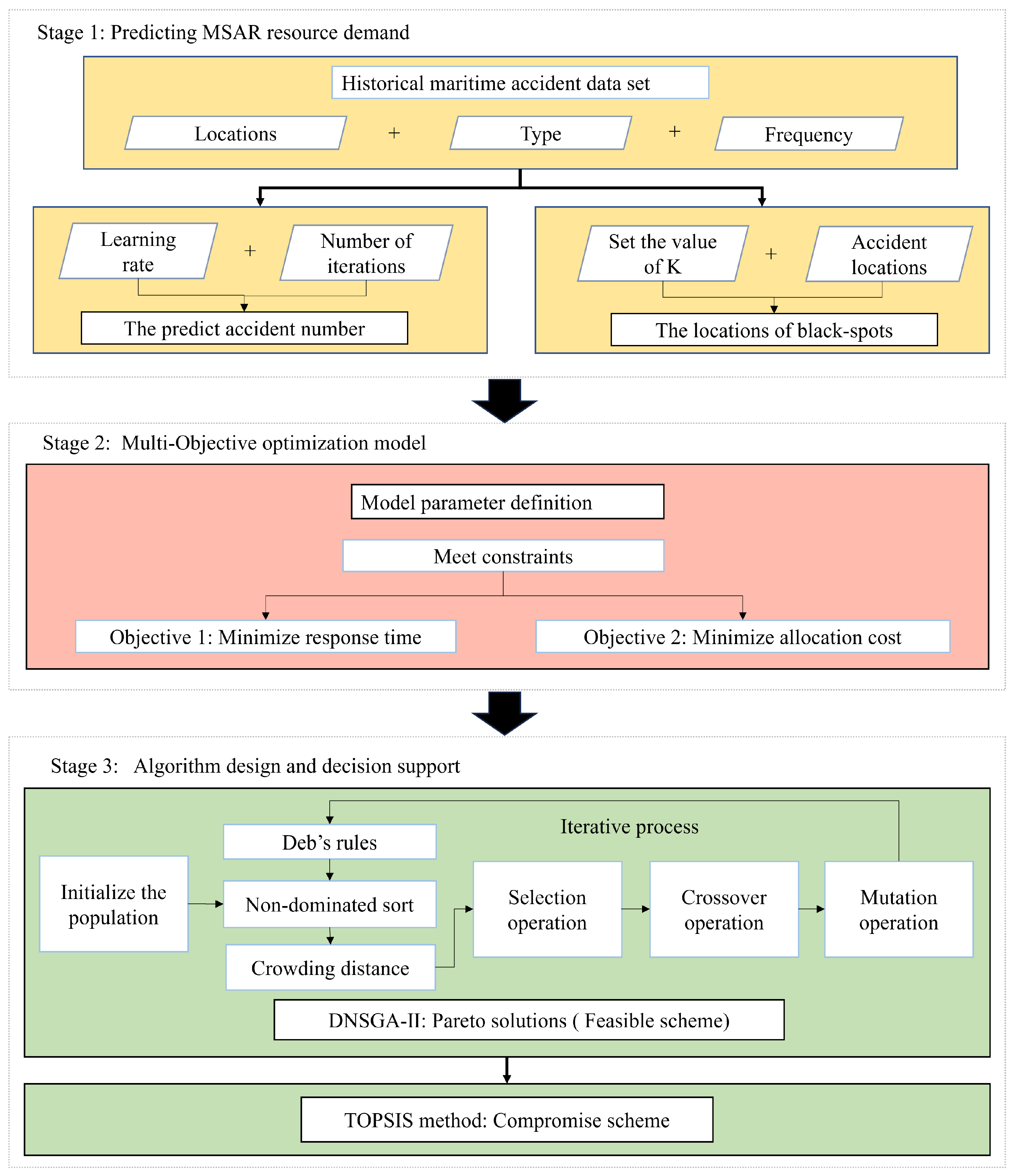
3. Model and Methods

Figure 1 shows the framework of our MSAR resource allocation optimization method. In Stage 1, based on the historical maritime accident data, we utilize LSTM and the K-medoids algorithm to predict the number of accidents and identify the accident black spots for the next year. The prediction methods are discussed in Section 3.1. The predicted number of accidents is crucial for determining the necessary MSAR resources. Next, we discuss the concept of MSAR resource allocation. We then introduce the variables in the model and establish a multi-objective optimization model for MSAR resource allocation in Stage 2. Finally, we provide a detailed explanation of the steps to solve the model using the DNSGA-II and apply the TOPSIS method to select the compromise solution from the Pareto solutions in Stage 3.

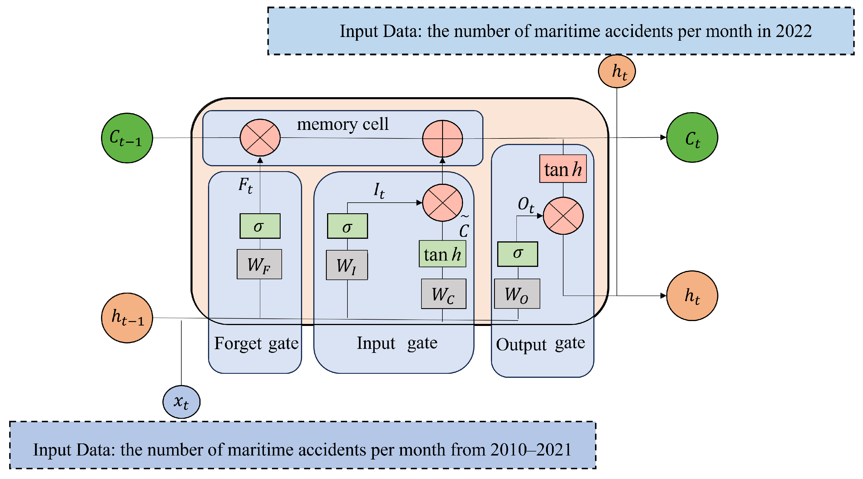
3.1. Prediction of Demand for MSAR Resources

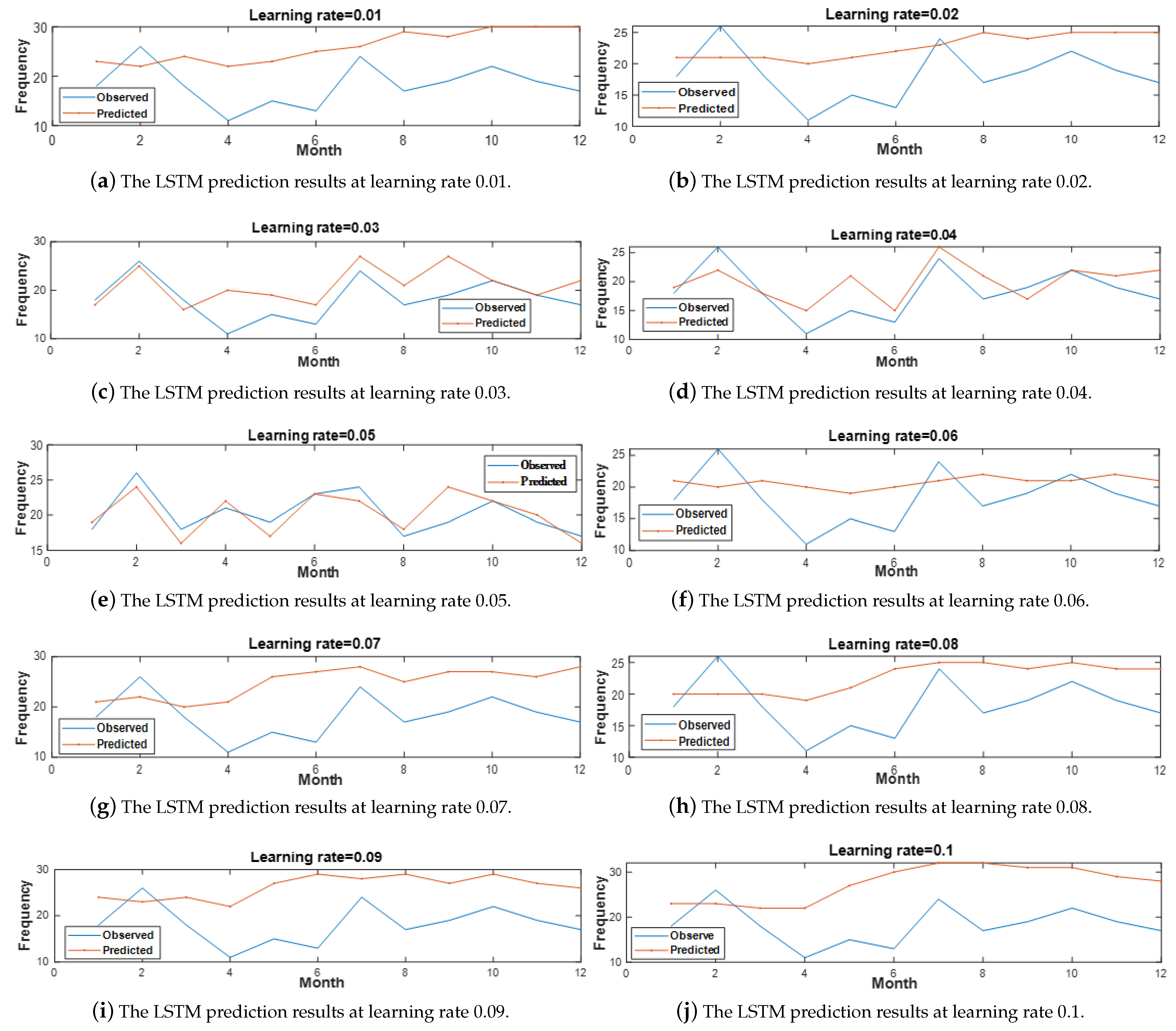
3.1.1. LSTM

LSTM is a type of temporal recurrent neural network and is an extension of the recurrent neural network. LSTM can efficiently store or discard information by employing gate mechanisms, significantly enhancing its memory capacity. The remarkable memory capability of LSTM enables it to converge more quickly when dealing with long sequence problems, thereby avoiding some common issues, like long-term dependencies, gradient explosions, and gradient vanishing, that typically arise in conventional recurrent neural networks. LSTM is highly proficient in predicting time-series data [34]. Through time-series analysis of historical maritime accident data, LSTM can unveil seasonal patterns, long-term trends, and cyclic variations in accident frequency. Besides these attributes, LSTM can capture nonlinear relationships within the data. In contrast, simple statistical methods might struggle to capture these nonlinear relationships due to their limitations in dealing with complex data patterns. Figure 2 illustrates the structure of the LSTM network.

In this paper, we initially divide the historical maritime accident data from 2010 to 2021 into monthly intervals. The frequency of accidents occurring each month is recorded as $O_i\in O$, forming a time-series dataset, denoted as $O=(O_1,O_2,\dots ,O_i,\dots ,O_m)$, where m is the collection node. Then, we employ LSTM to learn $O=(O_1,O_2,\dots ,O_i,\dots ,O_m)$ and obtain the number of maritime accidents that occurred each month in 2022.

Each LSTM cell introduces a memory cell $C_t$ in addition to the regular output from each unit $h_t$ and incorporates three gates: the forget gate, input gate, and output gate [35]. The forget gate, described by Equations (1) and (2), determines whether the information from each time step should be retained or discarded. The input gate controls the amount of new information added to the cell, represented by Equations (3)–(5). The state of the cell at the current time is represented by Equation (6). Lastly, the output gate, defined in Equations (7) and (8), controls the amount of information transmitted from the current state of the cell to the current hidden state, where $F_t$, $I_t$, and $O_t$ are the values of the forget gate, input gate, and output gate, respectively. $x_t$ is the input value at the current moment. $h_{t-1}$ represents all the outputs of the model from the previous moment. $W_F$, $W_I$, and $W_O$ are the weight matrices of the forget gate, input gate, and output gate, respectively, whereas $b_F$, $b_I$, and $b_O$ are the bias quantities for the forget gate, memory gate, and output gate, respectively. $W_C$ represents the weight matrices of the candidate vector, and $b_C$ is the bias quantity of the candidate vector. $C_t$ represents the candidate vectors at the t-th time step. $\tilde{C}$ is the temporary memory cell. The final output of the LSTM is $H_t$.

$$F_t=\sigma (W_F·[h_{t-1},x_t]+b_F)$$

(1)

$$\sigma =\frac{1}{1-e^x}$$

(2)

$$I_t=\sigma (W_I·[h_{t-1},x_t]+b_I)$$

(3)

$$\tilde{C}=\tan h(W_C·[h_{t-1},x_t]+b_C)$$

(4)

$$\tan =\frac{e^x-e^{-x}}{e^x+e^{-x}}$$

(5)

$$C_t=f_t·C_{t-1}+i_t·{\tilde{C}}_t$$

(6)

$$O_t=\sigma (W_O·[h_{t-1},x_t]+b_O)$$

(7)

$$H_t=O_t·\tan h\left(C_t\right)$$

(8)

3.1.2. K-Medoids

The K-medoids and K-means algorithms are distance-based clustering methods [36]. This type of method is widely used in traffic accident analysis due to its advantages, such as simplicity, practicality, and fast convergence. The K-means algorithm calculates the “mean” within clusters, whereas the K-medoids algorithm calculates the “median” within clusters. Therefore, the K-medoids algorithm exhibits greater robustness when dealing with noise and outliers. K-medoids can be divided into the following four steps:

Step 1: Construct a dataset $X=\left\{X_1,X_2,\dots ,X_n\right\}$ of historical maritime accidents; each object $X_i=(lo{n}_i,la{t}_i)$ includes two features: longitude and latitude. Subsequently, the dataset is divided into k clusters $P=\left\{P_1,P_2,\dots ,P_n\right\},k<n$. The selected accident black spot is $P_i=(lo{n}_i^p,la{t}_i^p)$.

Step 2: The K-medoids algorithm utilizes distance to measure the similarity between individuals. The common distance metrics include the Euclidean distance, Manhattan distance, Chebyshev distance, and Minkowski distance [36]. In this paper, we employ the Euclidean distance to quantify the similarity between individuals. Let $dis$ denote the Euclidean distance between the sample points. We assign each point to the cluster whose center is closest to it.

$$dis(X_i,P_i)=\sqrt{{(lo{n}_i^p-lo{n}_i)}^2+{(la{t}_i^p-la{t}_i)}^2}$$

(9)

Step 3: Select a non-accident black-spot sample $X_{random}$ to replace an accident black spot $P_i$ and compute the sum of intra-cluster distances E using Equation (10). If the value decreases, replace the accident black spot $P_i$ with the new sample $X_{random}$, forming a new set of accident black spots.

$$E=\sum _{i\in k}^{}\sum _{s\in P}^{}dis(s,P_i)$$

(10)

Step 4: Repeat steps 2 and 3 until the updated accident black spots no longer change, concluding the clustering process and generating the final set of k-determined accident black spots.

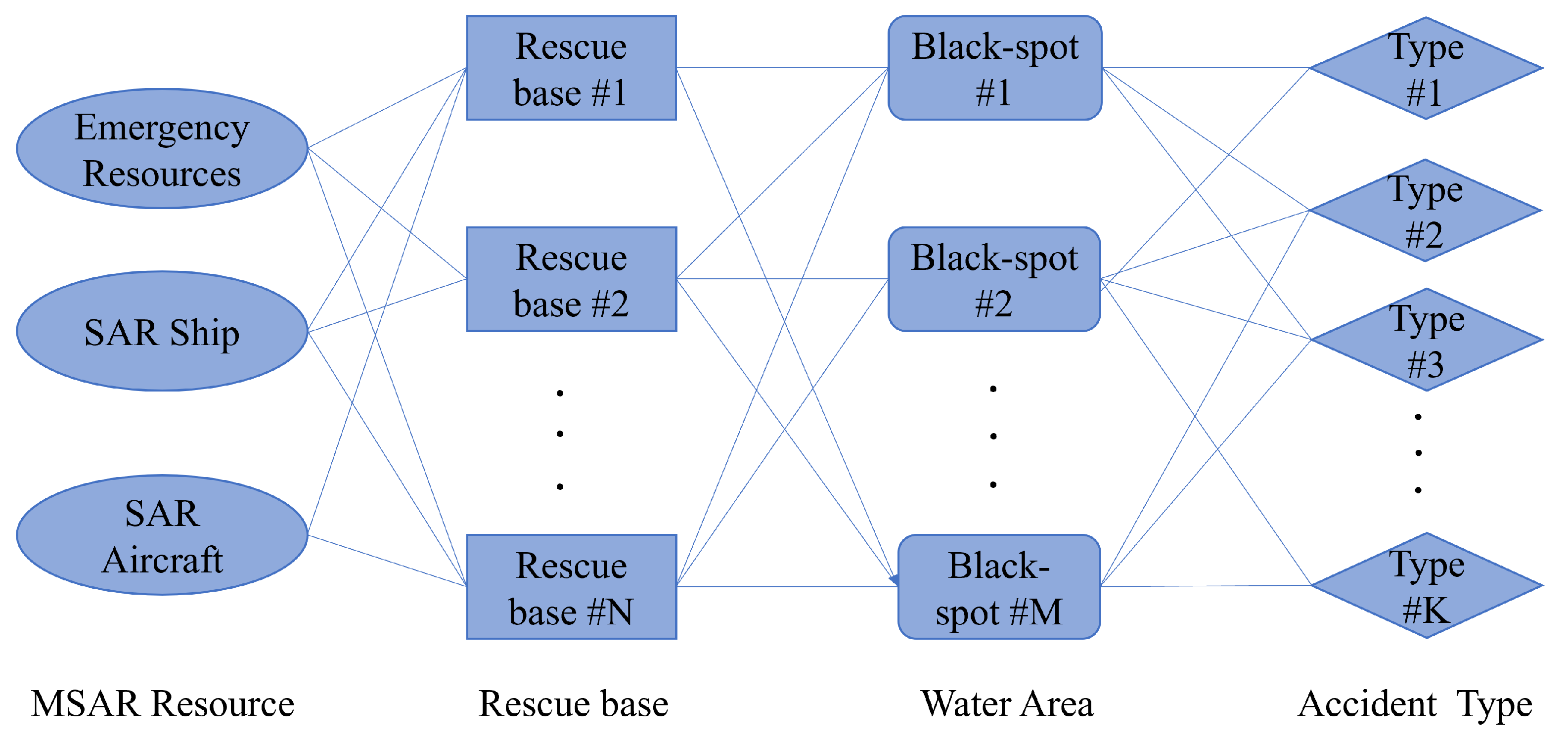
3.2. Multi-Objective Optimization Model

3.2.1. Problem Description

The occurrence of maritime accidents is difficult to predict in advance, often accompanied by challenges such as difficulties in ensuring human survival, marine environmental pollution, and property losses. To initiate emergency rescue operations as early as possible and thereby reduce the impact of the accident, the command center must promptly and efficiently allocate sufficient MSAR resources to the accident area based on the specific circumstances of the accident. Typically, the available rescue equipment includes rescue ships and rescue aircraft. Effective collaboration between these two types of equipment can increase the probability of successful maritime rescue missions. Conversely, inadequate rescue resources at the rescue base can lead to missing the critical window for rescue. There are two core issues related to maritime emergency response support: (1) predicting the numbers and types of accidents in the sea for the next year and determining the locations of potential accident black spots, and (2) efficiently allocating various MSAR resources to multiple rescue bases, considering multiple constraints such as resource limitations, rescue base capacity, and accident demand. The optimized allocation should aim to minimize response time and costs. To deal with such problems, we establish an MSAR resource allocation model in this section.

Figure 3 illustrates the concept of MSAR resource allocation. The emergency resources (e.g., water, life jackets, etc.), rescue ships (e.g., tugboats, fireboats, etc.), and rescue aircraft used in the MSAR process are collectively referred to as MSAR resources. The widely accepted definition of accident black spots was proposed by the authors of [37], who stated that “a location is considered an accident black spot if its expected accident occurrence rate is higher than the accident rate in similar locations”. While this definition is comprehensive in its consideration, it places a greater emphasis on guidance rather than practical application. In this paper, the concept of an accident black spot extends beyond an isolated accident to encompass a point that reflects the distribution characteristics of accidents in the surrounding maritime area [38].

We propose four assumptions for the MSAR resource allocation model:

(1)

Rescue bases are not allowed to borrow rescue resources from each other.

(2)

Rescue aircraft and ships must depart from their respective rescue bases to carry out rescue missions. To ensure the effectiveness of the model, we consider the worst-case scenario where there is no available rescue equipment near the accident black spot.

(3)

Rescue ships and aircraft do not experience malfunctions during rescue missions.

(4)

The rescue mission cannot be interrupted by unexpected factors such as adverse weather conditions or successful self-rescue.

3.2.2. Notations and Definitions

Based on the problem description, we establish a multi-objective optimization model. We provide specific descriptions of the sets and indices, normal parameters, and decision variables. It should be noted that, except for the variables related to the actual allocation of MSAR resources by the rescue bases ($Y{Q}_{ik,c}$, $Y{Q}_{ia,c}$, and $Y{Q}_{ib,c}$) and the actual provision of MSAR resources to accident black spots ($R{Q}_{idk,ct}$, $R{Q}_{ida,ct}$, and $R{Q}_{idb,ct}$), all other parameters can be obtained from historical data and the results of the LSTM network and the K-medoids algorithm.

Sets and indexes:

$a\in A$: Set of MSAR aircraft types.

$b\in B$: Set of MSAR ship types.

$k\in K$: Set of emergency resources.

$e\in E$: Set of accident types.

$d\in D$: Set of accident black spots.

$i\in I$: Set of rescue bases.

Normal parameters:

$S_{de}$: The forecasted number of accidents e in accident black spot d.

$Y_e$: Threshold of the number of accidents e.

$P_{ek}$: The number of emergency resources k required for accident e.

$P_{ea}$: The number of MSAR aircraft a required for accident e.

$P_{eb}$: The number of MSAR ships b required for accident e.

$F{Q}_{dk,c}$: The number of emergency resources k required for black spot d.

$F{Q}_{da,c}$: The number of MSAR aircraft a required for black spot d.

$F{Q}_{dbi,c}$: The number of MSAR ships b required for black spot d.

$M{Q}_{ik}$: The maximum number of emergency resources k that rescue base i can hold.

$M{Q}_{ia}$: The maximum number of MSAR aircraft a that rescue base i can hold.

$M{Q}_{ib}$: The maximum number of MSAR ships b that rescue base i can hold.

$UNA$: Total number of MSAR aircraft.

$UNB$: Total number of MSAR ships.

$V_a$: The speed of MSAR aircraft a.

$V_b$: The speed of MSAR ship b in still water.

${\Omega }_i$: Weight of storage emergency resources at base i.

$L{T}_{id}$: Distance between rescue base i and the location of black spot d.

$T_{id}$: Response time coefficient of rescue base i to black spot d.

$R_a$: The unit transportation cost of MSAR aircraft a.

$R_b$: The unit transportation cost of MSAR ship b.

$C_{ik}$: The maintenance cost of emergency resources k at rescue base i.

$C_{ia}$: The maintenance cost of MSAR aircraft a at rescue base i.

$C_{ib}$: The maintenance cost of MSAR ship b at rescue base i.

$C{S}_i$: Fixed cost of rescue base i.

$YC$: Transportation cost.

$BC$: Storage cost.

$GC$: Fixed cost.

${\theta }_{1-3}$: The function of ${\theta }_{1-3}$ is to unify dimensions.

Decision variables:

${\varphi }_{id,a}$: 1, if MSAR aircraft a at rescue base i provides rescue services to accident black spot d, and 0 otherwise, $i\in I$, $d\in D$.

${\varphi }_{id,b}$: 1, if MSAR ship b at rescue base i provides rescue services to accident black spot d, and 0 otherwise, $i\in I$, $d\in D$.

$R{Q}_{idk,ct}$: The actual number of emergency resources k provided by rescue base i to accident black spot d.

$R{Q}_{ida,ct}$: The actual number of MSAR aircraft a provided by rescue base i to accident black spot d.

$R{Q}_{idb,ct}$: The actual number of MSAR ships b provided by rescue base i to accident black spot d.

$Y{Q}_{ik,c}$: The actual number of emergency resources k equipped at rescue base i.

$Y{Q}_{ia,c}$: The actual number of MSAR aircraft a equipped at rescue base i.

$Y{Q}_{ib,c}$: The actual number of MSAR ships b equipped at rescue base i.

3.2.3. Objective Functions and Constraints of the Multi-Objective Model

In this model, the first objective is to minimize the emergency response time, as expressed in Equation (11). The second objective is to minimize the allocation cost, as expressed in Equations (12)–(15). The constraints are expressed in Equations (16)–(21).

Objective functions:

$$\begin{array}{c}\hfill \min f_1={\theta }_1\sum _{i\in I}^{}\sum _{d\in D}^{}{T}_{id}+{\theta }_2\sum _{i\in I}^{}\sum _{d\in D}^{}\sum _{k\in K}^{}{\alpha }_{id}{T}_{id}Y{Q}_{ik,c}-{\theta }_{3}lg\sum _{i\in I}^{}\sum _{d\in D}^{}{T}_{id}\end{array}$$

(11)

$$\begin{array}{c}\hfill \min f_2=YC+BC+GC\end{array}$$

(12)

$$\begin{array}{c}\hfill YC=\sum _{i\in I}^{}\sum _{d\in D}^{}(\sum _{a\in A}^{}\frac{{\varphi }_{id,a}R{Q}_{ida,ct}L{T}_{id}}{V_a}{R}_a+\sum _{b\in B}^{}\frac{{\varphi }_{id,b}R{Q}_{idb,ct}L{T}_{id}}{V_b}{R}_b)\end{array}$$

(13)

$$\begin{array}{c}\hfill BC=\sum _{i\in I}^{}(\sum _{k\in K}^{}{\Omega }_i{C}_{ik}Y{Q}_{ik,c}+\sum _{a\in A}^{}{C}_{ia}Y{Q}_{ia,c}+\sum _{b\in B}^{}{C}_{ib}Y{Q}_{ib,c})\end{array}$$

(14)

$$\begin{array}{c}\hfill GC=\sum _{i\in I}^{}C{S}_i\end{array}$$

(15)

Constraints:

$$\begin{array}{c}\hfill T_{id}=\max \left\{\max \frac{{\varphi }_{id,a}L{T}_{id}}{V_a},\max \frac{{\varphi }_{id,b}L{T}_{id}}{V_b}\right\},\forall i\in I,d\in D,a\in A,b\in B\end{array}$$

(16)

$$\begin{array}{c}\hfill F{Q}_{dk,c}=\sum _{e\in E}^{}\sum _{k\in K}^{}\left[\frac{S_{de}}{Y_e}\right]P_{ek},F{Q}_{da,c}=\sum _{e\in E}^{}\sum _{a\in A}^{}\left[\frac{S_{de}}{Y_e}\right]P_{ea},F{Q}_{db,c}=\sum _{e\in E}^{}\sum _{b\in B}^{}\left[\frac{S_{de}}{Y_e}\right]P_{eb},\forall i\in I,d\in D,k\in K,a\in A,b\in B\end{array}$$

(17)

$$\begin{array}{c}\hfill 0\le R{Q}_{idk,ct}\le Y{Q}_{ik,c}\le M{Q}_{ik},\forall i\in I,d\in D,k\in K\end{array}$$

(18)

$$\begin{array}{c}\hfill S_d\le R{Q}_{ida,ct}\le Y{Q}_{ia,c}\le MA{Q}_i,S_d\le R{Q}_{idb,ct}\le Y{Q}_{ib,c}\le MB{Q}_i,\forall i\in I,d\in D,a\in A,b\in B\end{array}$$

(19)

$$\begin{array}{c}\hfill F_{dk,c}\le \sum _{i\in I}^{}R{Q}_{idk,ct},F_{da,c}\le \sum _{a\in A}^{}R{Q}_{ida,ct},F_{db,c}\le \sum _{b\in B}^{}R{Q}_{idb,ct},\forall i\in I,d\in D,k\in K,a\in A,b\in B\end{array}$$

(20)

$$\begin{array}{c}\hfill 0\le \sum _{i\in I}^{}\sum _{d\in D}^{}\sum _{a\in A}^{}R{Q}_{ida,ct}\le UNA,0\le \sum _{i\in I}^{}\sum _{d\in D}^{}\sum _{b\in B}^{}R{Q}_{idb,ct}\le UNB,\forall i\in I,d\in D,a\in A,b\in B\end{array}$$

(21)

In the above optimization model, Equation (11) represents the efficiency objective, mainly consisting of three parts. The first part is the response time of the rescue forces. The second part is the response time of the emergency supplies, aiming to minimize response time while meeting the emergency response requirements to accidents. The third part is the safety index of the accident black spot, which is proportional to the shortest response time for the accident black spot. The safety index indicates that the accident black spot with a shorter response time is considered safer.

Equations (12)–(15) represent the economic objective, where the allocation cost consists of three parts. The first part concerns the transportation cost of resources. This cost refers to the expenses involved in transporting MSAR resources from their bases to accident black spots. It can ensure that more rescue forces are allocated to rescue bases closer to accident black spots. The second part is the storage cost of MSAR resources. The third part is the fixed costs required for maintaining the rescue resources at each base. These costs do not include the expenses associated with conducting SAR actions at the accident site once the MSAR resources have arrived.

Equation (16) is used to calculate the response time of rescue base i to accident black spot d. The response time refers to the time it takes for all the rescue equipment dispatched from rescue base i to reach accident black spot d. Equation (17) is used to calculate the type and number of emergency resources, MSAR ships, and MSAR aircraft required for accident black spot d. Equation (18) indicates that the number of emergency resources provided by rescue base i to accident black spot d cannot exceed the amount stored within the rescue base itself, and the stored quantity of emergency supplies within rescue base i cannot surpass its capacity. Equation (19) indicates that when providing MSAR ships and aircraft to accident black spot d, rescue base i needs to consider the different accident types at black spot d. This constraint ensures that suitable rescue equipment is available for each type of accident. Moreover, the number of MSAR ships and aircraft dispatched to black spot d from rescue base i cannot exceed the total amount of rescue equipment stored at rescue base i. In addition, the amount of rescue equipment stored at rescue base i cannot surpass the available berth capacity. Equation (20) indicates that the total number of MSAR resources provided by all rescue bases to each accident black spot cannot be less than the predicted amount of MSAR resources required for that accident black spot. Equation (21) states that the total amount of rescue equipment dispatched by all rescue bases cannot exceed the actual amount of rescue equipment available within the entire maritime area.

3.3. Algorithm Design and Decision Support

3.3.1. DNSGA-II

This paper deals with constrained multi-objective optimization problems. When dealing with multi-objective problems involving complex constraints, the traditional ant colony and particle swarm algorithms often encounter challenges, such as becoming trapped in local optima and exhibiting poor convergence for Pareto solutions. To achieve more reasonable global optimal solutions, we adopt the non-dominated sorting genetic algorithm II (NSGA-II) with Deb’s rules to solve the multi-objective allocation problem of MSAR resources. The NSGA-II is a multi-objective optimization algorithm based on genetic algorithms [39]. It utilizes a global optimal approximation approach to obtain a Pareto-optimal solution set for multiple objectives, providing decision makers with various preference options. The NSGA-II is widely favored for solving bi-objective and tri-objective optimization problems due to its rapid execution and strong convergence properties.

It should be noted that the traditional one-dimensional real-number encoding used in the NSGA-II is inconsistent with the two-dimensional compositional nature of the multi-objective allocation problem for MSAR resources discussed in this paper. In addition, the strict supply–demand constraints defined in Equations (18)–(21) make it easy for individuals in the NSGA-II’s evaluation process to violate these constraints and become infeasible. Therefore, building upon the original algorithm, we have developed a two-dimensional integer vector encoding scheme and integrated Deb’s rules. This enhancement aims to improve the NSGA-II’s performance in solving the allocation problem. The fundamental steps of the proposed DNSGA-II are outlined below:

Step 1: Randomly generate an initial population, where each individual is represented by a two-dimensional integer vector with constraints (18) and (19).

Step 2: Compute the objective function value of each individual in the initial population according to Equations (11)–(15).

Step 3: Utilize a fast, non-dominated ordering mechanism based on the objective function values of each individual to sort the initial population, followed by the computation of crowding distances for each individual.

Step 4: Utilize the roulette wheel selection mechanism; individuals are chosen from the initial population. Subsequently, the selected individuals undergo crossover and mutation using partial matching crossover techniques and random exchange techniques [40], resulting in the generation of the evolved population.

Step 5: Calculate the objective function values for each individual in the evolved population.

Step 6: Combine the initial and evolved populations into a single composite population, and then conduct environmental selection. Utilize the fast, non-dominated sorting mechanism to rank the composite population based on the objective function values and compute the crowding distances for each individual. Subsequently, select a number of the best individuals from the composite population based on their non-dominated ranks and crowding distances to form a new initial population.

Step 7: If the algorithm reaches the termination condition (e.g., maximum iteration count), stop the evolution and output the current initial population. Otherwise, proceed to Step 4 to continue the evolution of the initial population.

Regarding the evolutionary mechanism of the NSGA-II, specific details can be found in the literature [39] and are not reiterated here. To further elucidate the scope of this paper’s work, a detailed explanation is provided below for the two-dimensional integer vector encoding scheme and Deb’s constraint dominance criteria.

Individual coding scheme: The multi-objective allocation problem of MSAR resources discussed in this paper primarily focuses on the allocation of R types of MSAR resources among I rescue bases to meet the emergency needs of D accident black spots. This problem exhibits the typical characteristics of a two-dimensional combinatorial optimization problem. After the combination of the practical aspects of MSAR resource allocation and the encoding characteristics of the NSGA-II, we design a two-dimensional integer vector encoding scheme, represented by Equation (22), to define the candidate solutions.

In individual A, each row represents rescue base $I_i$, and each column represents accident black spot $H_d$. The integer vector $W_{id}$ in row i and column d represents the allocation of MSAR resources from rescue base $I_i$ to black spot $H_d$. If $W_{id}>0$, rescue base $I_i$ is involved in the rescue of black spot $H_d$ and contributes $W_{id}$ units of MSAR resources. Conversely, if $W_{id}=0$, rescue base $I_i$ does not participate in the rescue operation at black spot $H_d$ and does not provide any MSAR resources for $H_d$. When initializing each individual in the population, we apply Equation (23) for $\forall i\in I,d\in D,r\in K\cup A\cup B$.

$$A=\left[\begin{array}{cccc}{W}^{11}& W^{12}& \cdots & W^{1d}\\ W^{21}& W^{22}& \cdots & W^{2d}\\ ⋮& ⋮& \ddots & ⋮\\ W^{i1}& W^{i2}& \cdots & W^{id}\end{array}\right]$$

(22)

$$\left\{\begin{array}{c}{w}_r^{id},\forall r\in K\leftarrow rand(0,\min \left\{Y{Q}_{ik,c},F{Q}_{dk,c}\right\})\\ w_r^{id},\forall r\in A\leftarrow rand(0,\min \left\{Y{Q}_{ia,c},F{Q}_{da,c}\right\})\\ w_r^{id},\forall r\in B\leftarrow rand(0,\min \left\{Y{Q}_{ib,c},F{Q}_{db,c}\right\})\end{array}\right.$$

(23)

It can be observed that each individual generated initially satisfies constraints (18) and (19) but may not necessarily satisfy constraints (20) and (21). Even if some individuals initially satisfy all constraints, they may potentially violate these constraints after undergoing crossover and mutation operations, rendering them infeasible. When a significant number of infeasible individuals appear in the population, the convergence and search efficiency of the algorithm are significantly reduced. Therefore, we employ constraint violation degrees in non-dominated sorting to increase the probability of eliminating infeasible solutions, encouraging each individual to approach the feasible region rapidly and enhancing the capability of the algorithm to explore feasible solutions.

Deb’s constraint dominance criteria: The optimal individuals are chosen based on two types of information: Pareto dominance and constraint violation degree. For feasible solutions, we apply the fast, non-dominated sorting mechanism. For infeasible solutions that violate the constraints, we utilize the constraint violation value ($CV$) to measure the extent of constraint violation quantitatively [41]. Solutions with a higher $CV$ are more likely to be eliminated, whereas solutions with a lower $CV$ are more likely to be retained in the next-generation population. The $CV$ of infeasible solutions is calculated using Equations (24) and (25), where G represents the number of inequality constraints, K represents the number of equality constraints, $g\left(x\right)$ represents the inequality constraints, and $CV\left(x\right)$ represents the equality constraints.

$$C{V}_x=\sum _{g\in G}^{}{g}_g\left(x\right)+\sum _{k\in K}^{}\left|h_k\left(x\right)\right|$$

(24)

$$g_x=\left\{\begin{array}{cc}0& g_x⩾0\\ -g_x& g_x<0\end{array}\right.$$

(25)

3.3.2. Multi-Attribute Decision Optimization-Based Method

In multi-objective optimization problems, decision makers often face a dilemma in selecting the optimal solution because each non-dominated solution corresponds to different optimal values for each objective function. To assist in this decision-making process, we utilize the Technique for Order Preference by Similarity to Ideal Solution (TOPSIS) to rank the optimization solutions. This approach allows decision makers to select the compromise solution from the Pareto solution set. The main steps are as follows:

Step 1: Calculate objective weights $W^o$. Construct a decision matrix $G={\left(g_{ij}\right)}_{m\times n}$, $i\in [1,m],j\in [1,n]$, composed of Pareto-optimal solutions. Normalize the decision matrix $G={\left(g_{ij}\right)}_{m\times n}$ to $G^{{}^{\prime }}={\left(g_{ij}^{{}^{\prime }}\right)}_{m\times n}$ using Equation (26). Compute the entropy value $h_j$ of the j-th optimization objective using Equation (27), and compute the objective weights using Equation (28), where m is the number of Pareto solutions.

$$g_{ij}^{{}^{\prime }}=\frac{\max \left(g_{ij}\right)-g_{ij}}{\max \left(g_{ij}\right)-\max \left(g_{ij}\right)}$$

(26)

$$h_j=-\frac{1}{ln\left(m\right)}\sum _{i=1}^m{y}_{ij}ln\left(y_{ij}\right),y_{ij}=\frac{g_{ij}^{{}^{\prime }}}{{\sum }_{i=1}^m{g}_{ij}^{{}^{\prime }}}$$

(27)

$$W_j^o=-\frac{1-h_j}{m-{\sum }_{i=1}^m{h}_j}$$

(28)

Step 2: Calculate the subjective and objective weight ratio coefficients $u^s$ and $u^o$ using Equation (29), where $k=0.5$ is the equilibrium coefficient.

$$\left\{\begin{array}{c}{u}^s=\exp (-\left[1+\frac{k{\sum }_{i=1}^m{\sum }_{j=1}^n{w}_j^s(1-g_{ij}^{{}^{\prime }})}{(1-k)}\right])\\ u^o=\exp (-\left[1+\frac{k{\sum }_{i=1}^m{\sum }_{j=1}^n{w}_o^s(1-g_{ij}^{{}^{\prime }})}{(1-k)}\right])\end{array}\right.$$

(29)

Step 3: Calculate the combined weight $W=[w_1,w_2,\cdots ,w_j,\cdots ,w_r]$, where the components of W satisfy Equation (30).

$$W_j=\frac{u^s}{u^s+u^o}{W}_j^s+\frac{u^o}{u^s+u^o}{W}_j^o$$

(30)

Step 4: Calculate the normalized weighted matrix $Z_{ij}={\left(z_{ij}\right)}_{m\times n}={(w_j·g_{ij}^{{}^{\prime }})}_{m\times n}$ based on Equations (26) and (30), and obtain the positive ideal solution vector $S^{+}$ and the negative ideal solution vector $S^{-}$ using Equation (31).

$$\left\{\begin{array}{c}{S}^{+}=[z_1^{+},z_2^{+},\cdots ,z_n^{+}]=\min \left(z_{ij}\right)\\ S^{-}=[z_1^{-},z_2^{-},\cdots ,z_n^{-}]=\max \left(z_{ij}\right)\end{array}\right.$$

(31)

Step 5: Calculate the Euclidean distance $d_i^{+}$ and $d_i^{-}$ between the feasible solution and $S^{+}$ and $S_i^{-}$.

$$\left\{\begin{array}{c}{d}_i^{+}=\sqrt{{\sum }_j^n{(z_j^{+}-z_{ij})}^2}\\ d_i^{-}=\sqrt{{\sum }_j^n{(z_j^{-}-z_{ij})}^2}\end{array}\right.$$

(32)

Step 6: Calculate the relative proximity $D_i$ between each optimization solution and the ideal solution.

$$D_i=\frac{d_i^{-}}{d_i^{+}+d_i^{-}}$$

(33)

Step 7: Optimization scheme selection. We rank the feasible solutions in descending order according to their $D_i$. The solution with a larger $D_i$ is closer to the optimal solution. The solution with the maximum $D_i$ represents our selected compromise solution.

4. An Application of the Proposed Methodology

The South China Sea is one of the world’s busiest maritime transportation routes. Its unique natural environment and geographical location contribute to a higher possibility of accidents compared to other maritime regions. Therefore, in this section, we utilize historical maritime accident data and MSAR resource information from the South China Sea to conduct simulation experiments. We aim to validate the model and method presented in this paper through the following experiments.

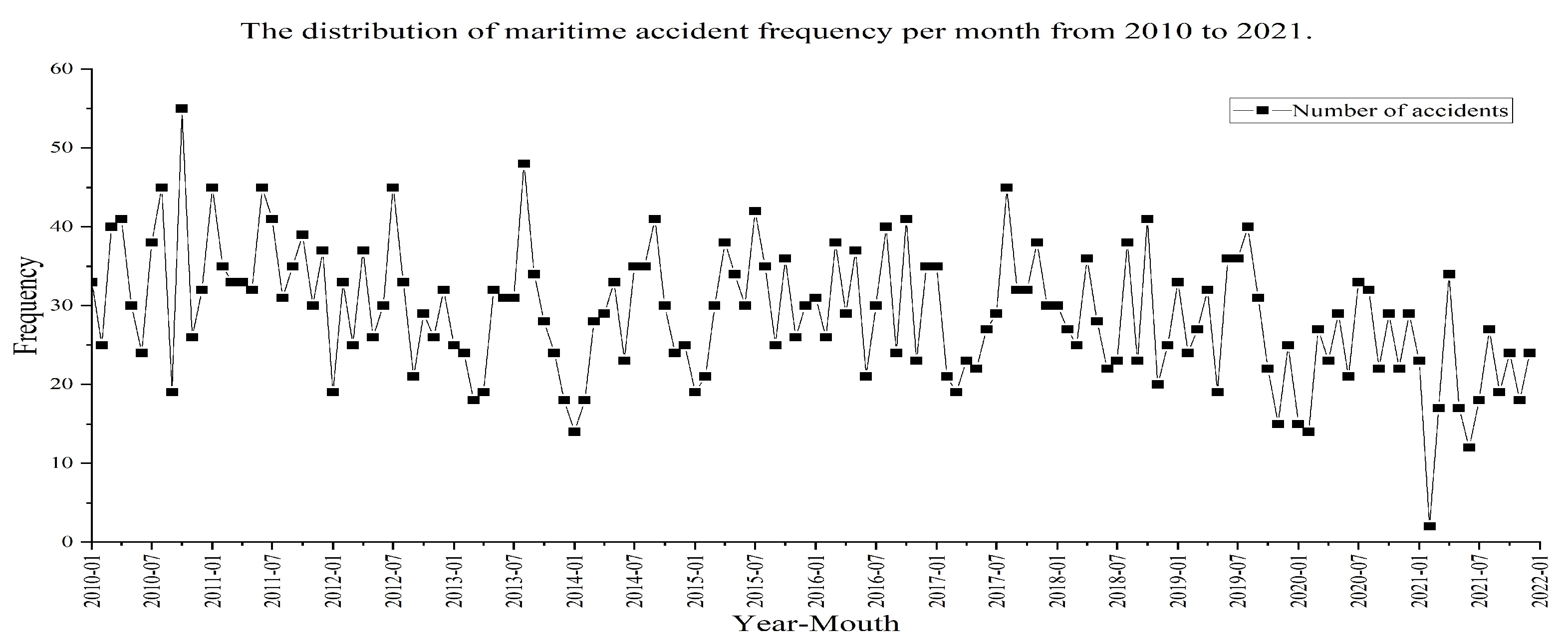
4.1. Prediction of MSAR Resources

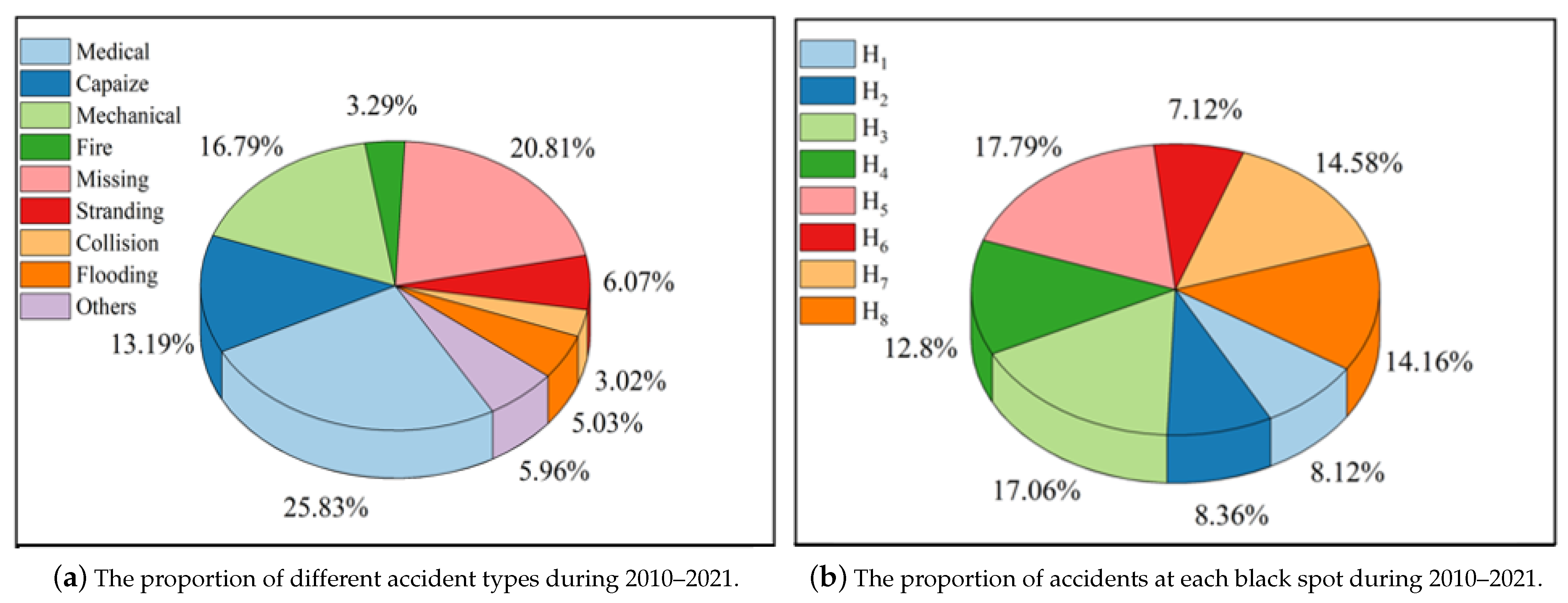
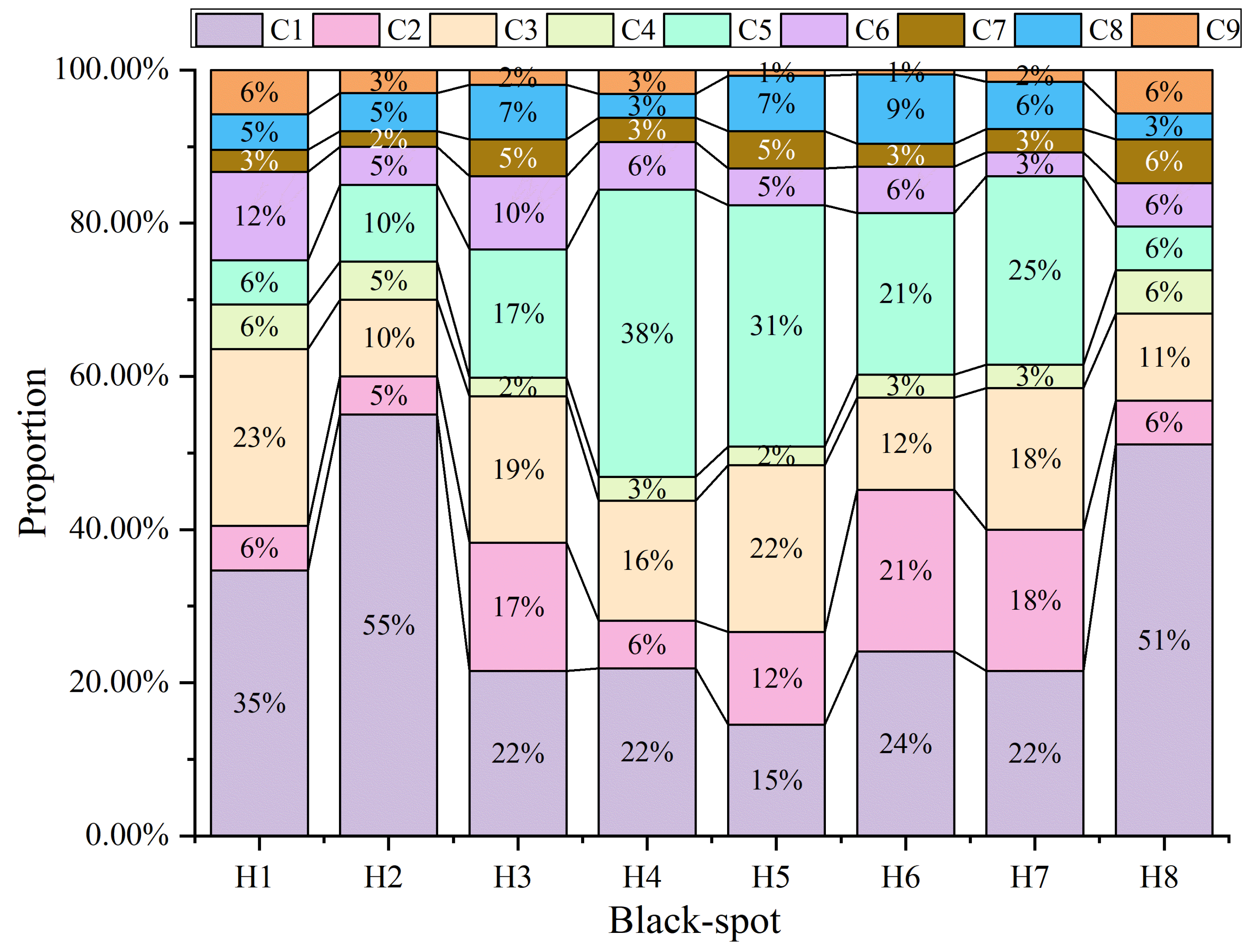
4.1.1. Maritime Accident Prediction

Data Preparation: We collected and organized the frequency of accidents that occurred in the South China Sea every month from 2010 to 2021, as presented in Figure 4. It can be observed that the number of accidents was higher in February, March–April, July–August, and October. These fluctuations were primarily influenced by weather and environmental factors in the South China Sea. For instance, the frequent influence of cold air in February, thick sea fog during March–April, frequent typhoons in July–August, and the dry northeast monsoon in October contributed significantly. In addition, other factors like shallow waters, reefs, and coral reefs also contributed to the increased occurrence of accidents.

Evaluation Criteria for Prediction Performance: The mean absolute percentage error (MAPE) and root-mean-squared error (RMSE) are commonly employed metrics used to evaluate the quality of model predictions [34]. The MAPE measures the relative deviation between predicted and actual values but cannot directly obtain the magnitude of differences between them. In contrast, the RMSE can quantify the absolute error between predicted and actual values, complementing the limitations of the MAPE. The combination of the two evaluation criteria can offer a more comprehensive assessment of a model’s predictive performance. The MAPE and RMSE are expressed in Equations (34) and (35), where N is the sample size, $X_i$ is the i-th actual value, and $Y_i$ is the i-th predicted value:

$$MAPE=\frac{1}{N}\sum _{j=1}^N\left|\frac{X_i-Y_i}{X_i}\right|$$

(34)

$$RMSE=\sqrt{\frac{{\sum }_{j=1}^N{(X_i-Y_i)}^2}{N}}$$

(35)

LSTM training: We divided the collected data into a training set and a test set in a 9:1 ratio, which served as the input for the LSTM model to predict the monthly accident counts in the South China Sea for the year 2022. The learning rate is a crucial parameter for the LSTM model, as it controls the speed of network learning and convergence and significantly influences the prediction results. To achieve the best prediction results, we conducted experiments with different learning rates (ranging from 0.01 to 0.1), keeping the number of iterations (250), input layer nodes (1), and output layer nodes (1) constant. Figure 5 shows the prediction results as the learning rate increased from 0.01 to 0.1.

To intuitively compare the errors of the models, we summarize the MAPE and RMSE values at different learning rates in

Table 2. The prediction errors of LSTM at different learning rates.

No.	1	2	3	4	5	6	7	8	9	10
Learning rate	0.01	0.02	0.03	0.04	0.05	0.06	0.07	0.08	0.09	0.1
MAPE	8.4167	5.4440	3.5315	2.6721	1.5839	4.1607	7.2514	5.3333	8.5214	9.75
RMSE	9.0784	6.0553	4.4064	3.2404	1.9758	4.6904	8.0881	6.0415	9.2195	10.5633

. The table reveals that the prediction error consistently decreased as the learning rate increased from 0.01 to 0.05. However, the error started to rise when the learning rate increased from 0.05 to 0.07. Subsequently, the error decreased at a learning rate of 0.08 and increased again as the learning rate reached 0.1. Consequently, it can be deduced that with learning rates of 0.05 and 0.08, the error reached a local optimization. In contrast, the predictive model with a learning rate of 0.05 achieved fewer errors between the two local optimal solutions. Therefore, we selected the predicted result with a learning rate of 0.05 for further analysis in this paper.

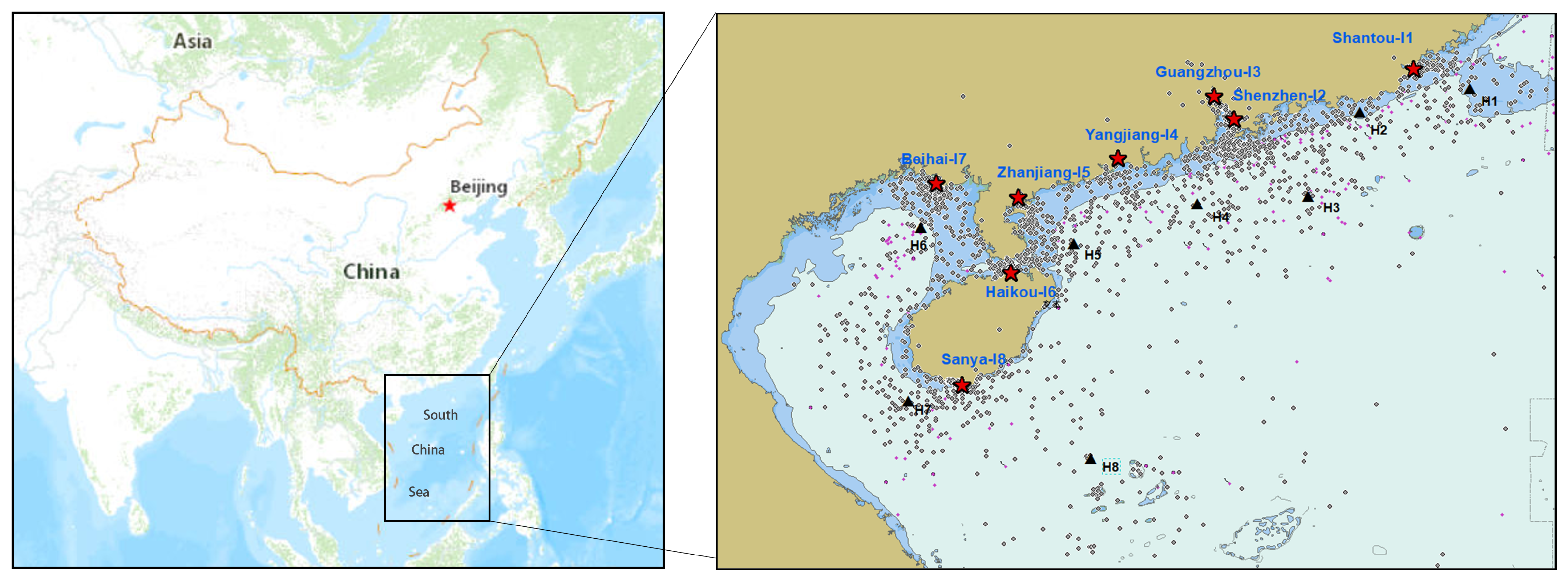
4.1.2. Identification of Maritime Accident Black Spots

We present the historical accident data in the South China Sea from 2010 to 2021 on a nautical chart. In Figure 6, each black point represents an accident; some accidents that occurred in sensitive maritime areas are not shown. It can be observed that the South China Sea features numerous and relatively dispersed islands. Areas near the coastline exhibit a higher frequency of accidents, whereas regions farther from the coastline experience fewer accidents due to the lower shipping traffic.

We utilized the K-medoids algorithm to cluster the accident data, resulting in the identification of eight accident black spots. The black spots in various regions are denoted by black triangles ($H_1$–$H_8$). The rescue bases are the following: Shantou base ($I_1$), Shenzhen base ($I_2$), Guangzhou base ($I_3$), Yangjiang base ($I_4$), Zhanjiang base ($I_5$), Haikou base ($I_8$), Beihai base ($I_7$), and Sanya base ($I_8$). Their locations are represented by red stars.

Figure 7a illustrates the distributions of various types of maritime accidents from 2010 to 2021, including medical rescues ($C_1$), capsizes ($C_2$), mechanical failures ($C_3$), fires ($C_4$), missing persons ($C_5$), ship groundings ($C_6$), collisions ($C_7$), and ship flooding ($C_8$). The proportions of each type of maritime accident are as follows: $C_1$ (25.83%); $C_2$ (13.19%); $C_3$ (16.79%); $C_4$ (3.29%); $C_5$ (20.81%); $C_6$ (6.07%); $C_7$ (3.02%); and $C_8$ (5.03%). Figure 7b shows the proportions of accidents in each accident black spot, whereas Figure 8 displays the distribution of the different types of accidents in each accident black spot. Based on the prediction results, clustering outcomes, and statistical data, we determined the number of each type of accident occurring at each accident black spot for the year 2022, as presented in

Table 3. The number of each different type of accident occurring at each accident black spot for the year 2022.

Black Spot	Number of Predicted Accidents
	${\mathit{C}}_{\mathbf{1}}$	${\mathit{C}}_{\mathbf{2}}$	${\mathit{C}}_{\mathbf{3}}$	${\mathit{C}}_{\mathbf{4}}$	${\mathit{C}}_{\mathbf{5}}$	${\mathit{C}}_{\mathbf{6}}$	${\mathit{C}}_{\mathbf{7}}$	${\mathit{C}}_{\mathbf{8}}$
$H_1$	6	1	4	1	1	2	0	0
$H_2$	11	1	2	1	2	1	0	1
$H_3$	9	7	8	1	7	4	2	3
$H_4$	7	2	5	1	12	2	1	1
$H_5$	6	5	9	1	13	2	2	3
$H_6$	8	7	4	1	7	2	1	3
$H_7$	7	6	6	1	8	1	1	2
$H_8$	9	1	2	1	1	1	1	0

. For example, the numbers of the eight types of accidents at black spot $H_1$ are 6, 1, 4, 1, 1, 2, 0, and 0, respectively.

4.2. MSAR Resource Allocation Optimization

4.2.1. Test Case

We chose the rescue bases and MSAR resource data in the South China Sea as the basis for our simulation experiments.

Table 4. The location of each rescue base and accident black spot.

Rescue Base	Lon. (E)	Lat. (N)	Black Spot	Lon. (E)	Lat. (N)
Shantou ($I_1$)	116.45	23.18	$H_1$	117.41	22.57
Shenzhen ($I_2$)	113.52	22.31	$H_2$	115.54	22.33
Guangzhou ($I_3$)	113.33	22.52	$H_3$	115.01	21.11
Yangjiang ($I_4$)	112.00	21.52	$H_4$	113.18	21.08
Zhanjiang ($I_5$)	110.24	21.15	$H_5$	111.18	20.24
Haikou ($I_6$)	110.16	20.01	$H_6$	108.49	20.43
Beihai ($I_7$)	109.04	21.28	$H_7$	108.38	17.55
Sanya ($I_8$)	109.3	18.13	$H_8$	111.34	17.01

provides the latitude and longitude coordinates for each rescue base and accident black spot. Detailed information on the available rescue equipment at each rescue base is listed in

Table 5. Detailed information on MSAR resources.

No.	MSAR Equipment	Quantity	Speed (km/h)	Transportation Cost (EUR/h)
1	Marine professional rescue ship ($B_1$)	10	34.26	500
2	Medium endurance multitasked ship ($B_2$)	4	51.39	1000
3	MSAR lifeboat ($B_3$)	19	59.62	1000
4	EC225 helicopter ($A_1$)	2	275	1800
5	S-76C helicopter ($A_2$)	3	287	1600

, including the quantities, driving speeds, and transportation costs.

Table 6. Emergency storage quantity of different emergency resources.

	${\mathit{I}}_1$	${\mathit{I}}_2$	${\mathit{I}}_3$	${\mathit{I}}_4$	${\mathit{I}}_5$	${\mathit{I}}_6$	${\mathit{I}}_7$	${\mathit{I}}_8$
$K_1$	125	120	135	119	85	76	124	180
$K_1$	178	154	216	221	168	154	263	336
$K_1$	127	164	186	81	157	120	330	312
$K_1$	108	90	49	80	54	46	111	154
${\Omega }_i$	0.8	0.9	0.85	0.95	1.1	1.25	1.15	1.2
$C{S}_i$	7890	4740	5749	4700	7800	9890	6785	8452

offers insights into the fixed costs, maximum storage capacities, and storage coefficients for the four types of emergency resources allocated to each rescue base. Specifically, water ($K_1$) is 10 gallons/unit, food ($K_2$) is 5 packs/unit, life jackets ($K_4$) are 10/unit, and medical kits ($K_4$) are 1/unit.

Table 7. The amount of MSAR resources required for different types of maritime accidents and the price of MSAR resources.

Accident Type	Emergency Resources				MSAR Equipment
	${\mathit{K}}_{\mathbf{1}}$	${\mathit{K}}_{\mathbf{2}}$	${\mathit{K}}_{\mathbf{3}}$	${\mathit{K}}_{\mathbf{4}}$	${\mathit{A}}_{\mathbf{1}}$	${\mathit{A}}_{\mathbf{2}}$	${\mathit{B}}_{\mathbf{1}}$	${\mathit{B}}_{\mathbf{2}}$	${\mathit{B}}_{\mathbf{3}}$
$C_1$	2	5	1	4	1	0	0	0	0
$C_2$	4	6	15	3	0	1	0	0	1
$C_3$	4	10	10	2	0	0	1	0	0
$C_4$	10	16	2	1	0	0	1	0	0
$C_5$	2	4	5	2	0	1	0	0	1
$C_6$	2	10	10	2	0	0	0	1	0
$C_7$	10	10	12	1	0	0	1	0	0
$C_8$	6	10	15	3	0	0	1	0	0
Maintenance cost	(EUR/unit)				(EUR/year)
	60	60	5	20	2000	2000	1200	1500	1800

presents the resource requirements for the eight accident types and the fixed costs of allocating each MSAR resource, as summarized in [42].

We determined the thresholds for each type of accident based on the recommendations of maritime safety experts. The thresholds for accident categories $C_1$–$C_8$ are as follows: 10, 6, 10, 8, 6, 5, 3, and 8. Typically, accidents involving medical rescue, capsize, and missing persons require urgent aircraft dispatch for support. The thresholds for rescue aircraft for $C_1$, $C_2$, and $C_5$ are 35, 30, and 30, respectively.

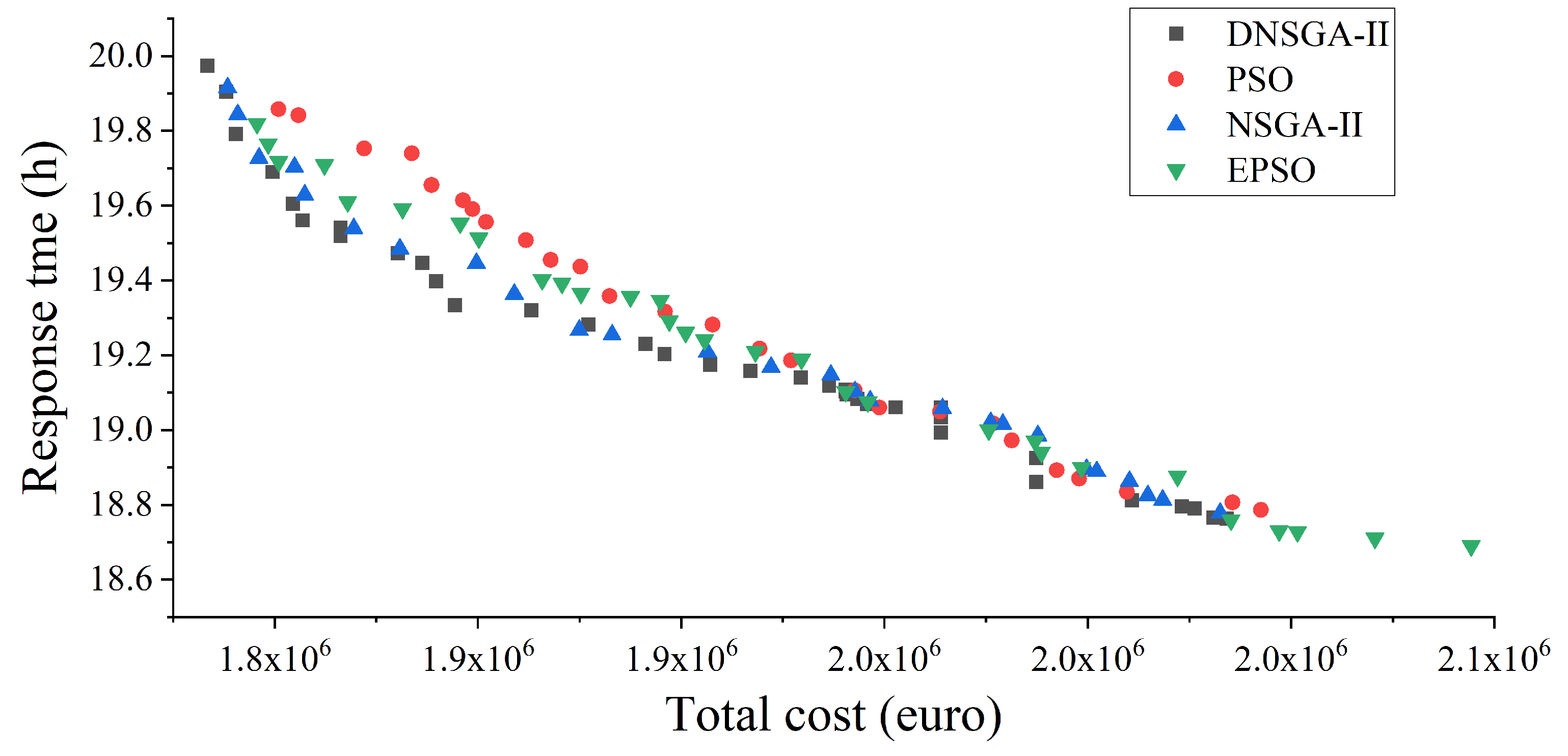
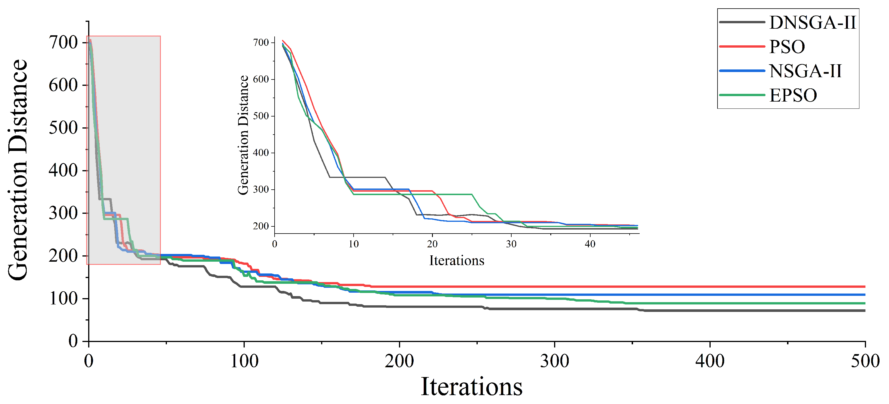
4.2.2. Performance Evaluation

The DNSGA-II described in Section 3.3.1 was programmed using MATLAB 2022b. To verify the efficiency of the DNSGA-II, we also employed the NSGA-II and the particle swarm optimization algorithm to solve the problems discussed in this paper. Furthermore, we compared the existing MSAR allocation algorithm (enhanced particle swarm optimization, EPSO [32]) with our model. For the NSGA-II and DNSGA-II, we set the population size, maximum iterations, crossover rate, and mutation rate to 50, 500, 0.9, and 0.1, respectively. In the PSO algorithm [14], we set the number of particles to 50. The maximum number of iterations was set to 500. The maximum particle velocity was set to 0.15. Both learning factors were set to 2.0. The maximum and minimum values for the inertia weight were set to 0.9 and 0.4, respectively. We adopted the parameter settings for EPSO from [32], with 6000 iterations and 80 particles. The inertia weight, individual learning rate, and group learning rate were set to 0.9, 0.8, and 0.3, respectively.

These numerical experiments were implemented using a computer with an Intel(R) Core(TM) i5-13400FCPU @ 2.50 gigahertz and 16 gigabytes of RAM. To obtain the approximate solutions for the problem, we conducted ten independent runs using the DNSGA-II, NSGA-II, PSO, and EPSO algorithms. The integrated Pareto frontiers resulting from the ten runs are presented in Figure 9.

To further assess and compare the performance of the four algorithms (DNSGA-II, NSGA-II, PSO, and EPSO), we chose the hyper-volume (HV) and quantity metric (QM). The HV was designed to calculate the volume of the region in the objective space enclosed by the non-dominated solution set and a reference point. It reflects the overall performance of an algorithm [43]. Equation (36) is the calculation formula for the HV, where $\sigma$ represents the Lebesgue measure, quantifying the volume of the region in the objective space; $\left|s\right|$ is the number of non-dominated solutions in the set; and $v_c$ represents the hyper-volume formed by the reference point and the c-th solution in the Pareto solution set. The QM measures the number of non-dominated feasible solutions obtained by an algorithm [44]. It represents the count of non-dominated solutions that satisfy all constraints, providing an intuitive measure of an algorithm’s exploration capability.

$$HV=\sigma ·U_{x=1}^{\left|s\right|}\left(v_c\right)$$

(36)

We ran each of the four algorithms ten times and then combined the solutions from the ten runs. Subsequently, we eliminated duplicate and dominated solutions to obtain a Pareto solution set for each algorithm in a single experiment. The performance of the three algorithms was compared using the HV metric (where $\overline{HV}$ is the average HV value, and $\widetilde{HV}$ is the standard deviation of HV), the QM metric, and the required CPU time (in seconds) for each algorithm’s Pareto solution set. The results for each algorithm in the HV metric were obtained by selecting the minimum values of the two objective functions as reference points.

Table 8. Performance comparison of DNSGA-II, PSO, NSGA-II, and EPSO.

No.	DNSGA-II				PSO				NSGA-II				EPSO
	$\overline{\mathit{HV}}$	$\widetilde{\mathit{HV}}$	QM	CPU(s)	$\overline{\mathit{HV}}$	$\widetilde{\mathit{HV}}$	QM	CPU(s)	$\overline{\mathit{HV}}$	$\widetilde{\mathit{HV}}$	QM	CPU(s)	$\overline{\mathit{HV}}$	$\widetilde{\mathit{HV}}$	QM	CPU(s)
1	742.31	22.58	37	384.32	698.23	27.54	28	313.5	716.24	24.83	28	346.60	725.64	23.67	31	326.41
2	743.45	23.21	36	384.94	697.54	26.78	27	312.93	718.43	25.21	29	344.02	715.8	23.58	28	324.57
3	738.42	23.67	33	372.23	697.54	27.41	27	312.93	717.92	24.92	29	348.02	716.58	22.57	31	326.86
4	745.32	22.53	42	383.02	695.32	25.81	27	312.34	721.23	24.31	28	342.93	718.26	24.57	34	326.58
5	743.28	23.51	40	394.28	694.83	28.13	24	314.63	715.92	25.63	25	346.11	725.14	23.54	32	332.15
6	747.26	24.24	41	396.92	695.83	27.62	23	314.02	718.72	24.92	27	345.23	719.68	23.54	32	325.24
7	753.45	24.65	36	384.49	697.38	27.71	23	313.52	715.32	23.51	28	345.42	721.24	24.15	34	329.45
8	745.54	23.16	37	384.76	696.45	27.65	26	313.65	717.10	24.89	28	346.26	724.64	24.61	29	330.15
9	752.62	23.49	35	382.65	697.29	27.16	29	314.31	715.92	24.71	30	348.35	721.54	22.44	31	326.54
10	734.92	21.53	39	386.56	695.24	28.52	27	312.89	719.23	23.96	25	347.32	715.64	23.61	29	324.59
Avg	744.66	23.26	37.67	388.42	695.17	27.43	26.33	313.45	717.60	24.69	27.78	346.16	720.42	23.63	31.1	327.25

presents the comparative results of the three algorithms, and the last row displays the average results (Avg) of the four evaluation metrics after 10 experiments. Specifically, the HV is a commonly used metric to measure the overall quality of a Pareto solution set obtained using multi-objective optimization algorithms. A larger $\overline{HV}$ indicates better quality in the obtained solutions using the algorithm. A smaller $\widetilde{HV}$ implies that the distribution of the solution set in the objective space exhibits relatively low fluctuations, indicating better stability of the algorithm. Regarding the QM, a larger QM value indicates a higher number of feasible solutions obtained, providing more choices for decision makers and signifying superior algorithm performance. In addition, there is no doubt that a smaller CPU value indicates that the algorithm solves the model more quickly.

Table 8 shows that for the multi-objective optimization model established in this paper, the DNSGA-II achieved the highest ($\overline{HV}=744.66$) and the smallest ($\widetilde{HV}=23.26$) values in the HV metric test results. In addition, in the QM metric results, the DNSGA-II achieved the highest QM value (43.67). Compared to the NSGA-II, PSO, and EPSO, the DNSGA-II generated higher-quality, non-dominated solutions with only $10.9$∼$19.3\%$ extra computation. The added time is not substantial and is acceptable relative to the degree of performance enhancement. The above experimental results indicate that under the drive of constraint dominance, the DNSGA-II can significantly reduce individual constraint violations, pushing individuals to evolve rapidly into the feasible region. In addition, the quality of the solutions obtained using the DNSGA-II is far superior to that of the other three algorithms, offering decision makers better and more diversified MSAR resource allocation solutions.

The convergence of algorithms is a crucial criterion for evaluating their performance, aiming to illustrate their capability to approach the optimal or desired solution [45]. We used the generation distance (GD) metric to assess the convergence performance of the algorithms. The GD value is the average Euclidean distance between each solution generated by the algorithm in each iteration and the known optimal solution. A smaller GD value implies that the solutions in the set are closer to the optimal solution. Figure 10 illustrates the iterative processes of the four algorithms. It can be observed that in the initial 40 iterations, all three algorithms converged rapidly. The DNSGA-II exhibited a lower GD than the other three algorithms. After a limited number of iterations, all algorithms tended to reach a stable state. The GD value for PSO stabilized at around 126 after the 182nd iteration, the GD value for the NSGA-II stabilized at around 109 after the 228th iteration, the GD value for EPSO stabilized at around 94 after the 344th iteration, and the GD value for the DNSGA-II stabilized at around 72 after the 355th iteration. The above results demonstrate that the DNSGA-II exhibits good convergence performance.

4.2.3. Computation Results

In Figure 9, it can be observed that, like most multi-objective optimizations, the Pareto solution set obtained using the DNSGA-II consists of multiple non-dominated solutions. Each solution in the Pareto solution set corresponds to an optimization plan and does not directly provide specific decisions for MSAR resource allocation. When the values of both objectives fall within an acceptable range, the optimal solution is selected based on the decision maker’s preference. Due to social responsibility, decision makers typically prioritize response efficiency over cost when making MSAR decisions.

Based on the Pareto-optimal solutions obtained using the DNSGA-II, we constructed a decision matrix of size 36 × 2. The objective weights $W^o=(0.6333,0.3667)$ were calculated using Equations (26)–(29), and subjective weights $W^s=(0.7,0.3)$ were assigned based on the experience of maritime security experts. According to Equation (32), the relative proximity of each individual in the Pareto-optimal solution set was computed.

The solution with the highest relative proximity value ($D_3$ = 0.9087) was chosen as the optimal solution. The optimal allocating scheme is shown in

Table 9. Emergency resource scheduling scheme.

	${\mathit{K}}_1$	${\mathit{K}}_2$	${\mathit{K}}_3$	${\mathit{K}}_4$	${\mathit{A}}_1$	${\mathit{A}}_2$	${\mathit{B}}_1$	${\mathit{B}}_2$	${\mathit{B}}_3$
$I_1$	98	173	125	79	1	0	1	0	1
$I_2$	82	152	133	89	0	1	2	1	3
$I_3$	96	143	129	45	0	0	1	1	2
$I_4$	101	181	69	79	0	1	2	0	2
$I_5$	85	152	145	52	0	0	1	0	0
$I_6$	62	148	137	36	0	0	1	0	1
$I_7$	116	236	248	87	1	0	1	0	1
$I_8$	167	302	306	135	0	1	1	1	3

. The response time value is 19.97 h, and the allocation cost is EUR 1.83 × 10⁶. It was found that the Guangzhou base ($I_2$) was relatively close to black spots $H_1$, $H_2$, and $H_3$, which is a key reason for the higher allocation of emergency resources and rescue forces. Similarly, the Sanya base ($I_8$) was closer to black spots $H_7$ and $H_8$, and given that black spot eight frequently experiences medical rescue ($C_1$) accidents, it also receives a larger allocation of rescue equipment.

To further validate the optimization capabilities of the model and algorithm proposed in this paper, we analyzed and compared the obtained optimal allocation scheme with the existing MSAR resource emergency response system in the South China Sea.

Table 10. The actual number of MSAR resources allocated to each rescue base in the South China Sea.

	${\mathit{K}}_1$	${\mathit{K}}_2$	${\mathit{K}}_3$	${\mathit{K}}_4$	${\mathit{A}}_1$	${\mathit{A}}_2$	${\mathit{B}}_1$	${\mathit{B}}_2$	${\mathit{B}}_3$
$I_1$	118	163	125	99	1	0	2	1	3
$I_2$	102	142	163	89	0	0	0	1	0
$I_3$	125	200	179	47	0	1	3	1	3
$I_4$	115	221	80	75	0	1	2	0	2
$I_5$	80	145	155	55	0	0	1	0	1
$I_6$	70	152	117	36	0	0	2	0	1
$I_7$	115	259	302	91	1	0	2	0	3
$I_8$	180	312	308	141	0	1	1	1	3

lists the actual allocation of MSAR resources to each rescue base in the South China Sea in 2022.

Table 11. Comparison of MSAR resource allocations before and after optimization.

	Before Optimization	After Optimization	Difference Percentage
Response time	22.52	19.97	−11.32%
Allocation cost	$1.95\times {10}^6$	$1.83\times {10}^6$	−6.15%
Number of MSAR ships	33	26	−21.21%
Number of MSAR aircraft	5	5	0
Number of $K_1$	905	807	−10.82%
Number of $K_2$	1594	1487	−6.71%
Number of $K_3$	1429	1292	−10.6%
Number of $K_4$	633	602	−4.90%

compares the costs, response times, and number of MSAR resources used before and after optimization. It can be seen that the allocation cost decreased by $6.15\%$ after optimization. In addition, due to the different allocations of rescue aircraft to rescue bases, the response time decreased by $11.32\%$. Furthermore, except for the quantity of rescue aircraft, the allocation of rescue ships decreased by $21.21\%$, and the amounts of the four types of emergency resources decreased by $10.82\%$, $6.71\%$, $10.6\%$, and $4.90\%$, respectively. The results of the case study validate the effectiveness of the multi-objective optimization method proposed in this paper. Moreover, compared to other methods, the solution obtained in this paper better balances efficiency and cost objectives, providing more effective decision support for MSAR resource allocation.

5. Conclusions

MSAR resource allocation is a fundamental prerequisite for prompt emergency response and rescue operations after maritime accidents. To meet the emergency requirements of maritime accidents, we analyzed and summarized relevant research work and proposed a comprehensive MSAR resource allocation method with the aim of improving timeliness and reducing costs. We employed LSTM to predict the number of maritime accidents and used the K-medoids algorithm to identify accident black spots that reflect the accident distribution characteristics of the sea area to determine the specific resource requirements for rescue. We also established a mathematical model that focuses on the configuration of the locations and quantities of four primary emergency resources, rescue ships, and aircraft for optimization, with the objective of minimizing response times and costs. Subsequently, we solved this model by employing the DNSGA-II. Finally, we proposed a multi-attribute decision optimization-based method for selecting the optimal MSAR equipment allocation. We applied the method to the South China Sea and analyzed MSAR missions in the South China Sea as a case study. The optimization results validate the feasibility and rationality of our method.

Compared to previous research, we incorporated additional content into our analysis: (1) We utilized the gathered raw data in a more sophisticated predictive model to forecast the number and types of future accidents. (2) We expanded the optimization objectives to include the allocation quantities of the four primary emergency resources and rescue equipment, considering multiple working capabilities and additional constraints to establish a comprehensive optimization model. (3) We addressed the problem of selecting an ideal solution that balances response efficiency and cost among the obtained non-dominant solutions. (4) We applied our model and algorithm to MSAR resource allocation in the South China Sea, addressing the issue of low overall emergency efficiency in the region. We compared the DNSGA-II with commonly used methods, such as NSGA-II, PSO, and EPSO, through multiple experiments. The results showed that, although the DNSGA-II has higher computational requirements, it demonstrates better stability and convergence. Furthermore, it can obtain solutions with shorter response times and lower allocation costs. Compared with the existing MSAR resource emergency response system, the optimized response time and allocation cost decreased by $11.32\%$ and $6.15\%$, respectively. The results validate the feasibility and rationality of our model and algorithm.

Although our method considers various real-world constraints and can be applied to maritime search and rescue resource allocation tasks, it also has some limitations. In practical applications, the allocation of MSAR resources is also affected by some other complex constraints, such as the impact of accident grade on demand for search and rescue resources and the influence of the marine environment on navigation speed. These complex constraints make the modeling and solving process challenging. In addition, we did not consider the role of islands in supporting SAR operations when selecting locations for the allocation of MSAR resources. In establishing the allocation model, we did not consider the costs incurred by the equipment involved in rescue operations. Furthermore, in maritime accident prediction, our method is solely based on historical accident data points, without considering the influence of environmental factors and maritime traffic flow. To enhance the applicability and rationality of our model, we plan to conduct further research on optimization problems that involve these constraints, thereby making the MSAR resource allocation plan more complex.

References

1. Baksh, A.A.; Abbassi, R.; Garaniya, V.; Khan, F. Marine transportation risk assessment using Bayesian Network: Application to Arctic waters. Ocean Eng. 2018, 159, 422–436. [Google Scholar] [CrossRef]
2. Knapp, S.; Heij, C. Evaluation of total risk exposure and insurance premiums in the maritime industry. Transp. Res. Part D Transp. Environ. 2017, 54, 321–334. [Google Scholar] [CrossRef]
3. Serra, M.; Sathe, P.; Rypina, I.; Kirincich, A.; Ross, S.D.; Lermusiaux, P.; Allen, A.; Peacock, T.; Haller, G. Search and rescue at sea aided by hidden flow structures. Nat. Commun. 2020, 11, 2525. [Google Scholar] [CrossRef] [PubMed]
4. Chen, J.; Di, Z.; Shi, J.; Shu, Y.; Wan, Z.; Song, L.; Zhang, W. Marine oil spill pollution causes and governance: A case study of Sanchi tanker collision and explosion. J. Clean. Prod. 2020, 273, 122978. [Google Scholar] [CrossRef]
5. Karatas, M. A dynamic multi-objective location-allocation model for search and rescue assets. Eur. J. Oper. Res. 2021, 288, 620–633. [Google Scholar] [CrossRef]
6. Tu, H.; Xia, K.; Mu, L.; Chen, X.; Wang, X. Predicting drift characteristics of life rafts: Case study of field experiments in the South China Sea. Ocean Eng. 2022, 262, 112–158. [Google Scholar] [CrossRef]
7. Cucco, A.; Quattrocchi, G.; Satta, A.; Antognarelli, F.; De Biasio, F.; Cadau, E.; Umgiesser, G.; Zecchetto, S. Predictability of wind-induced sea surface transport in coastal areas. J. Geophys. Res. Ocean. 2016, 121, 5847–5871. [Google Scholar] [CrossRef]
8. Vidan, P.; Hasanspahić, N.; Grbić, T. Comparative analysis of renowned softwares for search and rescue operations. Naše More Znan. časopis Za More I Pomor. 2016, 63, 73–80. [Google Scholar] [CrossRef]
9. Xiong, W.; Van Gelder, P.; Yang, K. A decision support method for design and operationalization of search and rescue in maritime emergency. Ocean Eng. 2020, 207, 107399. [Google Scholar] [CrossRef]
10. Galceran, E.; Carreras, M. A survey on coverage path planning for robotics. Robot. Auton. Syst. 2013, 61, 1258–1276. [Google Scholar] [CrossRef]
11. Bircher, A.; Kamel, M.; Alexis, K.; Burri, M.; Oettershagen, P.; Omari, S.; Mantel, T.; Siegwart, R. Three-dimensional coverage path planning via viewpoint resampling and tour optimization for aerial robots. Auton. Robot. 2016, 40, 1059–1078. [Google Scholar] [CrossRef]
12. Loree, N.; Aros-Vera, F. Points of distribution location and inventory management model for Post-Disaster Humanitarian Logistics. Transp. Res. Part E Logist. Transp. Rev. 2018, 116, 1–24. [Google Scholar] [CrossRef]
13. Choi, H.; Ha, H. The Priority of Supply Chain Designs for Humanitarian Relief with AHP (Analytic Hierarchy Process). Korean J. Logist. 2013, 21, 121–134. [Google Scholar] [CrossRef]
14. Hu, C.; Liu, X.; Hua, Y. A bi-objective robust model for emergency resource allocation under uncertainty. Int. J. Prod. Res. 2016, 54, 7421–7438. [Google Scholar] [CrossRef]
15. Mohammadi, M.; Mirzazadeh, A. MCLP and SQM models for the emergency vehicle districting and location problem. Decis. Sci. Lett. 2014, 3, 479–490. [Google Scholar] [CrossRef]
16. Alem, D.; Bonilla-Londono, H.F.; Barbosa-Povoa, A.P.; Relvas, S.; Ferreira, D.; Moreno, A. Building disaster preparedness and response capacity in humanitarian supply chains using the Social Vulnerability Index. Eur. J. Oper. Res. 2021, 292, 250–275. [Google Scholar] [CrossRef]
17. Liu, K.; Liu, C.; Xiang, X.; Tian, Z. Testing facility location and dynamic capacity planning for pandemics with demand uncertainty. Eur. J. Oper. Res. 2023, 304, 150–168. [Google Scholar] [CrossRef]
18. Sapankevych, N.I.; Sankar, R. Time series prediction using support vector machines: A survey. IEEE Comput. Intell. Mag. 2009, 4, 24–38. [Google Scholar] [CrossRef]
19. Li, O.; Liu, H.; Chen, C.; Rudin, C. Deep learning for case-based reasoning through prototypes: A neural network that explains its predictions. In Proceedings of the AAAI Conference on Artificial Intelligence, New Orleans, LA, USA, 2–7 February 2018; Volume 32. [Google Scholar]
20. Sun, J.; Cao, H.; Geng, B.; Tang, Z.; Li, X. Demand prediction of railway emergency resources based on case-based reasoning. J. Adv. Transp. 2021, 2021, 1–10. [Google Scholar] [CrossRef]
21. Jin, R.; Xia, T.; Liu, X.; Murata, T.; Kim, K.S. Predicting emergency medical service demand with bipartite graph convolutional networks. IEEE Access 2021, 9, 9903–9915. [Google Scholar] [CrossRef]
22. Zhu, X.; Zhang, G.; Sun, B. A comprehensive literature review of the demand forecasting methods of emergency resources from the perspective of artificial intelligence. Nat. Hazards 2019, 97, 65–82. [Google Scholar] [CrossRef]
23. Wagner, M.R.; Radovilsky, Z. Optimizing boat resources at the US Coast Guard: Deterministic and stochastic models. Oper. Res. 2012, 60, 1035–1049. [Google Scholar] [CrossRef]
24. Razi, N.; Karatas, M. A multi-objective model for locating search and rescue boats. Eur. J. Oper. Res. 2016, 254, 279–293. [Google Scholar] [CrossRef]
25. Akbari, A.; Pelot, R.; Eiselt, H.A. A modular capacitated multi-objective model for locating maritime search and rescue vessels. Ann. Oper. Res. 2018, 267, 3–28. [Google Scholar] [CrossRef]
26. Akbari, A.; Eiselt, H.A.; Pelot, R. A maritime search and rescue location analysis considering multiple criteria, with simulated demand. INFOR Inf. Syst. Oper. Res. 2018, 56, 92–114. [Google Scholar] [CrossRef]
27. Ma, Q.; Zhang, D.; Wan, C.; Zhang, J.; Lyu, N. Multi-objective emergency resources allocation optimization for maritime search and rescue considering accident black-spots. Ocean Eng. 2022, 261, 112178. [Google Scholar] [CrossRef]
28. Nelson, C.; Boros, E.; Roberts, F.; Rubio-Herrero, J.; Kantor, P.; McGinity, C.; Nakamura, B.; Ricks, B.; Ball, P.; Conrad, C.; et al. ACCAM global optimization model for the USCG aviation air stations. In Proceedings of the IIE Annual Conference. Proceedings. Institute of Industrial and Systems Engineers (IISE), Montreal, QC, Canada, 31 May–3 June 2014; p. 2761. [Google Scholar]
29. Karatas, M.; Razi, N.; Gunal, M.M. An ILP and simulation model to optimize search and rescue helicopter operations. J. Oper. Res. Soc. 2017, 68, 1335–1351. [Google Scholar] [CrossRef]
30. Ferrari, J.F.; Chen, M. A mathematical model for tactical aerial search and rescue fleet and operation planning. Int. J. Disaster Risk Reduct. 2020, 50, 101680. [Google Scholar] [CrossRef]
31. Guo, Y.; Ye, Y.; Yang, Q.; Yang, K. A multi-objective INLP model of sustainable resource allocation for long-range maritime search and rescue. Sustainability 2019, 11, 929. [Google Scholar] [CrossRef]
32. Sun, Y.; Ling, J.; Chen, X.; Kong, F.; Hu, Q.; Biancardo, S.A. Exploring maritime search and rescue resource allocation via an enhanced particle swarm optimization method. J. Mar. Sci. Eng. 2022, 10, 906. [Google Scholar] [CrossRef]
33. Zhou, X. A comprehensive framework for assessing navigation risk and deploying maritime emergency resources in the South China Sea. Ocean Eng. 2022, 248, 110797. [Google Scholar] [CrossRef]
34. Roondiwala, M.; Patel, H.; Varma, S. Predicting stock prices using LSTM. Int. J. Sci. Res. (IJSR) 2017, 6, 1754–1756. [Google Scholar]
35. Chen, K.; Zhou, Y.; Dai, F. A LSTM-based method for stock returns prediction: A case study of China stock market. In Proceedings of the 2015 IEEE International Conference on Big Data (Big Data), Santa Clara, CA, USA, 29 October–1 November 2015; IEEE: Piscataway, NJ, USA, 2015; pp. 2823–2824. [Google Scholar]
36. Shah, S.; Singh, M. Comparison of a time efficient modified K-mean algorithm with K-mean and K-medoid algorithm. In Proceedings of the 2012 International Conference on Communication Systems and Network Technologies, Rajkot, India, 11–13 May 2012; IEEE: Piscataway, NJ, USA, 2012; pp. 435–437. [Google Scholar]
37. Elvik, R. State-of-the-Art Approaches to Road Accident Black Spot Management and Safety Analysis of Road Networks; Transportøkonomisk Institutt: Oslo, Norway, 2007. [Google Scholar]
38. Zhang, J.; Wan, C.; He, A.; Zhang, D.; Soares, C.G. A two-stage black-spot identification model for inland waterway transportation. Reliab. Eng. Syst. Saf. 2021, 213, 107677. [Google Scholar] [CrossRef]
39. Srinivas, N.; Deb, K. Muiltiobjective optimization using nondominated sorting in genetic algorithms. Evol. Comput. 1994, 2, 221–248. [Google Scholar] [CrossRef]
40. Liu, D.; Yan, P.; Pu, Z.; Wang, Y.; Kaisar, E.I. Hybrid artificial immune algorithm for optimizing a Van-Robot E-grocery delivery system. Transp. Res. Part E Logist. Transp. Rev. 2021, 154, 102466. [Google Scholar] [CrossRef]
41. Babalik, A.; Cinar, A.C.; Kiran, M.S. A modification of tree-seed algorithm using Deb’s rules for constrained optimization. Appl. Soft Comput. 2018, 63, 289–305. [Google Scholar] [CrossRef]
42. Xiaolin, Z.; Changding, C. Multi-objective optimization of marine emergency resource dispatching. Navig. China 2019, 42, 56–62. [Google Scholar]
43. Duan, Y.; Ren, H.; Xu, F.; Yang, X.; Meng, Y. Bi-Objective Integrated Scheduling of Quay Cranes and Automated Guided Vehicles. J. Mar. Sci. Eng. 2023, 11, 1492. [Google Scholar] [CrossRef]
44. Rezaei, M.; Afsahi, M.; Shafiee, M.; Patriksson, M. A bi-objective optimization framework for designing an efficient fuel supply chain network in post-earthquakes. Comput. Ind. Eng. 2020, 147, 106654. [Google Scholar] [CrossRef]
45. Rashidnejad, M.; Ebrahimnejad, S.; Safari, J. A bi-objective model of preventive maintenance planning in distributed systems considering vehicle routing problem. Comput. Ind. Eng. 2018, 120, 360–381. [Google Scholar] [CrossRef]
Figure 1. The framework of the proposed optimized allocation method.
Jmse 12 00184 g001
Figure 2. The structure of LSTM.
Jmse 12 00184 g002
Figure 3. Diagram of MSAR resource allocation concept.
Jmse 12 00184 g003
Figure 4. The number of accidents that occurred in the South China Sea every month from 2010 to 2021.
Jmse 12 00184 g004
Figure 5. The LSTM prediction results at different learning rates.
Jmse 12 00184 g005
Figure 6. Locations of rescue bases and accident black spots.
Jmse 12 00184 g006
Figure 7. The distributions of accident types and accidents at each black spot during 2010–2021.
Jmse 12 00184 g007
Figure 8. Locations of rescue bases and accident black spots.
Jmse 12 00184 g008
Figure 9. Pareto frontier distributions of DNSGA-II, PSO, NSGA-II, and EPSO.
Jmse 12 00184 g009
Figure 10. The convergence processes of the algorithms.
Jmse 12 00184 g010