A Method for Clustering and Analyzing Vessel Sailing Routes Efficiently from AIS Data Using Traffic Density Images

Abstract

A vessel automatic identification system (AIS) provides a large amount of dynamic vessel information over a large coverage area and data volume. The AIS data are a typical type of big geo-data with high dimensionality, large noise, heterogeneous densities, and complex distributions. This poses a challenge for the clustering and analysis of vessel sailing routes. This study proposes an efficient vessel sailing route clustering and analysis method based on AIS data that uses traffic density images to transform the clustering problem of complex AIS trajectories into an image processing problem. First, a traffic density image is constructed based on the statistics of the preprocessed AIS data. Next, the main sea route regions of traffic density images are extracted based on local image features, geometric structures, and spatial features. Finally, the sailing trajectories are clustered using the extracted sailing patterns. Based on actual vessel AIS data, multimethod comparisons and performance analysis experiments are conducted to verify the feasibility and effectiveness of the proposed method. These experimental results reveal that the proposed method displays potential for the clustering task of challenging vessel sailing routes.

1. Introduction

With the continuous development of marine information technology, automatic identification system (AIS) equipment has been applied to ship navigation and has become one of the main navigational aids of ships. AIS is a system that can track and report the sailing status of ships, which is applied to maritime safety and communication between ships and shore and between ships and plays a significant role in maritime traffic management and ship navigation safety [1]. The AIS data contain the objective law of maritime traffic flow and have high application value. However, unlike vehicle trajectories on land, ships have high degrees of freedom when sailing, and AIS data are characterized by a large amount of data, large noise, heterogeneous densities, and complex distributions. This increases the difficulty of AIS data mining technology [2].

Vessel sailing route clustering was performed by analyzing the AIS records of the regions of interest. By clustering sailing routes, traffic flow information and traffic management references can be provided to the marine traffic supervision department. In addition, vessel sailing route clustering and analysis technologies are the foundation of sailing path planning [3,4], vessel trajectory prediction [5,6,7], and detection of abnormal trajectories [8,9].

The practical situation of this study mainly lies in the following aspects: First, the sea routes and the traffic flow characteristics of ships can be revealed, which have attracted wide attention in the shipping industry. Second, the clustered sea routes and their densities that can guide the ships’ navigation safety, which has always been the focus of continuous research in marine engineering. Furthermore, ship traffic monitoring can be performed, since main sea routes and sailing patterns are identified, and this is one of the biggest challenges in maritime law enforcement and emergency management. Hence, acquiring a ship’s route can help understand ship behaviors and reveal ship regular movement patterns, and it is of great significance for ship anomaly detection, route planning, navigation safety, and maritime situation awareness.

Currently, there are two main problems in vessel sailing route clustering. The first problem is the low computational efficiency and the inability to effectively conduct clustering with a large amount of uniform density data. The other problem is the similarity measurement of the trajectories; most measurement methods consider the global features of trajectories and ignore the overall motion trend or local features of ship trajectories.

The main difference between the local and global features of the trajectories is whether the entire trajectory or trajectory segments were used to calculate the similarity measurement. The global features of the trajectories mainly include the overall direction and motion trend, and the similarity measurement is calculated using the entire trajectory. Correspondingly, the local features of trajectories primarily consist of the characteristics (such as density and trend) of local trajectory segments, and the similarity measurement uses similar local features between trajectory segments.

To solve these problems, this study proposes an efficient vessel sailing route clustering and analysis method based on AIS data using traffic density images. The proposed method transforms a complex vessel sailing route clustering problem into an image-processing problem using traffic density images. The proposed method first constructs a traffic density image based on the statistics of preprocessed AIS data. Next, the main sea route regions of traffic density images are extracted based on local image features, geometric structures, and spatial features. Finally, the sailing trajectories are clustered using the extracted sailing patterns. The experimental results show that the proposed method can analyze over 293,868 AIS vessel trajectories with a Mallows score of over 0.81 in 584.1705 s.

The remainder of this paper is organized as follows: Section 2 introduces the existing work related to vessel trajectory clustering. Section 3 describes the proposed research methodology. Section 4 describes the experiments and results, including the experimental conditions, dataset introduction, performance comparison experiment, and time–space domain covering the experiment. Section 5 presents the application details and limitations of the proposed method. Finally, conclusions and future work are discussed in Section 6.

2. Literature Review

Related work on vessel trajectory clustering mainly uses similarity measurements of the trajectories or trajectory segments to perform clustering and analysis. Related methods are introduced as follows:

Currently, research on AIS trajectory clustering methods can be divided into two main categories: point-based clustering and trajectory-based clustering. The difference between the categories lies primarily in the different measurement methods for trajectory similarity or trajectory distance [10]. The point-based clustering method calculates the similarity of each trajectory point, which is easy to conduct but usually ignores the spatiotemporal correlation of vessel track points and is not conducive to the characterization of the overall motion characteristics of vessels [11,12]. The trajectory-based clustering method chooses the entire trajectory, or a trajectory segment composed of continuous trajectory points as the clustering object, and the similarity measure of the overall trajectory or the similarity measure of sub-trajectory segments is calculated [13,14]. The dynamic time warping (DTW) method, Hausdorff distance, and Frechet distance are commonly used to measure the similarities between trajectories. However, the DTW algorithm does not consider the characteristics of local trajectory segments, which may lead to over-stretching and over-compression [15,16]. The Hausdorff distance can identify the trajectory shape but ignores the timing features and direction of the trajectory, which is affected by trajectories near the transportation hub [17,18,19]. The Frechet distance can reflect the temporal characteristics of the trajectory and obtain better clustering results; however, it is not suitable for cluster analysis of long trajectory segments because of its high computational complexity [20].

After calculating the similarity measurement, clustering algorithms are used to determine the vessel sailing routes. Common clustering algorithms can be divided into the following categories: spatial clustering, hierarchical clustering, clustering based on density clustering, grid clustering, and model-based independent clustering algorithms [21]. The k-means method has the advantages of a simple process and fast calculation speed and is suitable for largescale datasets. However, it has poor processing ability for non-spherical clusters and is easily affected by the selection of initial cluster centers and the need to specify the number of clusters in advance [22,23,24]. Some widely used methods, such as the spectral clustering method, have disadvantages similar to those of the k-means method [25].

The density-based spatial clustering of applications with noise (DBSCAN) is one of the most widely used density-based clustering algorithms for analyzing AIS data [26]. The core idea of the DBSCAN algorithm is that a given data point belongs to a cluster if its density reaches a certain threshold; otherwise, it is considered a noise point. The DBSCAN method efficiently discovers clusters of arbitrary shapes and processes noisy data. In addition, it can automatically identify the number of clusters without specifying it in advance. However, DBSCAN faces challenges in terms of parameter sensitivity and time complexity. It has the problems of long clustering convergence time and low accuracy in the case of a large amount of data. Additionally, the clustering effect may be poor for datasets with large density differences. In addition, the hyperparameters of DBSCAN must be adjusted and optimized. To improve clustering performance, several studies have adopted many methods to determine the best parameters. Mohammad et al. proposed an adaptive DBSCAN method to identify clusters with varying densities; however, the number of data clusters must be predetermined, and the algorithm is less generalized [27]. Yang et al. proposed an adaptive semi-supervised method that uses both labeled and unlabeled data [28]. Liu et al. proposed a novel adaptive density trajectory cluster algorithm that computes the cluster radius using the density of the data distribution; however, the problem of time complexity remains [29]. Yaohui et al. introduced the concept of k-nearest neighbors and proposed an adaptive clustering algorithm to overcome the shortcomings of density peak-based clustering algorithms [30]. C Marques et al. proposed a clustered method to automatically perform a robust determination of cluster numbers and distributions; however, noisy data can be recognized [31]. Yang et al. proposed a density-based trajectory clustering of applications with noise (DBTCAN) algorithm to consider the spatiotemporal correlation between neighboring points on the same ship trajectory, which can be applied to pattern recognition of ship behavior in different ranges of waters [32]. Because the Hausdorff distance between every two trajectories is needed, the efficiency of DBTCAN is greatly reduced in large numbers of AIS data. Tang et al. proposed a FOLFST method to solve the problem of ignoring the overall motion trend or local features of ship trajectories [33], which also solved the problems of difficulty in parameter setting and sensitivity to a dataset with uneven density. However, the FOLFST still needs to simultaneously measure the similarity between the overall trajectories and calculate the single sub-trajectory distance, which requires more time. Yan et al. proposed a semantic extraction method for a large-area maritime route based on graph theory [34] that can be effectively used to analyze network characteristics, such as key nodes, edges, and network evolution. Waypoint analysis is important for this method.

In summary, most of the presented algorithms still face problems in that they cannot accurately identify noise and cannot effectively perform clustering with large amounts of uniform density data. To solve these problems, this study proposes an efficient vessel sailing route clustering and analysis method based on AIS data using traffic density images.

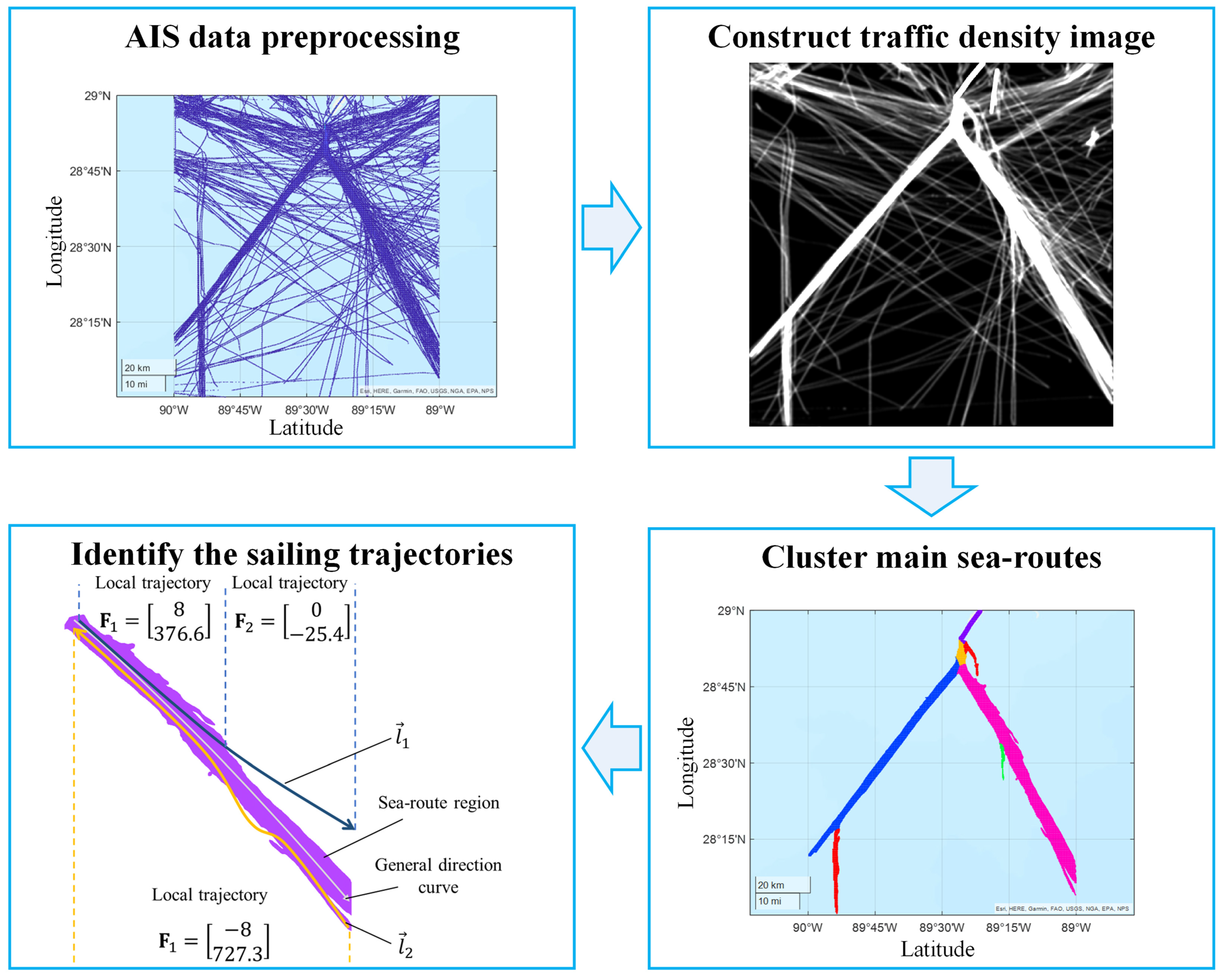
3. Research Methodology

In this section, the general framework of our method is introduced, and detailed descriptions of the key parts of our approach are presented.

The main sea route is defined as the stationary region where more ships sail. The general idea of the proposed traffic density image-based clustering method (TDIBC) is that the main sea routes should have a larger traffic flow density, which can be described using an image. The TDIBC process is shown in Figure 1. AIS data preprocessing consists mainly of data cleaning and interpolation. The traffic density image is constructed to transform the clustering problem of the AIS trajectories into an image processing problem, which can be effectively solved using computer vision methods. The main sea routes are clustered to determine the main sailing patterns in regions of interest. Finally, we can use these sailing patterns to identify sailing trajectories.

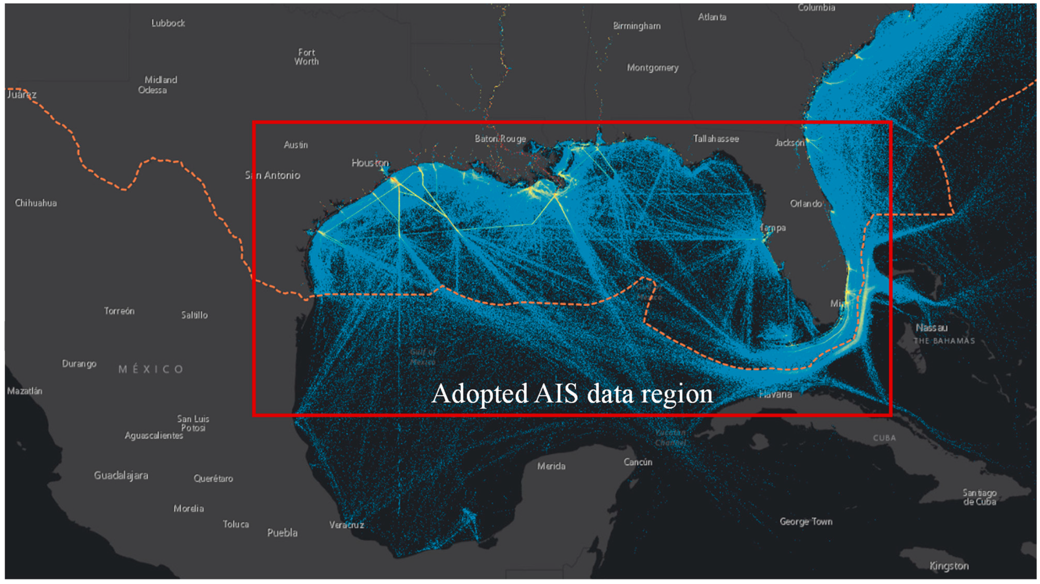
3.1. AIS Data Preprocessing

The AIS data are a typical type of big geodata. Influenced by equipment quality and protocol standards, AIS data have the following characteristics: different reporting frequencies and poor data quality. In general, the AIS data received in engineering practice are incomplete or inaccurate [35], and over 5% of the received AIS data are incorrect [36]. These abnormal AIS data are not conducive to the identification and supervision of a ship’s navigation intention and greatly reduce the application value of AIS data. It is necessary to perform AIS data preprocessing and remove abnormal data before analyzing the AIS data.

We first convert the geographic coordinate system into Mercator projection using Equation (1) as follows [37]:

$$\{\begin{array}{l}{r}_0=\frac{a\times \cos (l{a}_0)}{\sqrt{1-(e_1^2\times {\sin }^2(l{a}_0))}}\\ q=\ln \left(\tan (\frac{\pi }{4}+\frac{la}{2})\times {(\frac{1-e_1\times \sin (l{a}_0)}{1+e_1\times \sin (l{a}_0)})}^{\frac{e_1}{2}}\right)\\ x=r_0\times lo\\ y=r_0\times q\end{array}$$

(1)

Here, $(lo,la)$ represents the longitude and latitude coordinates of the original AIS point, $(x,y)$ is the coordinate after conversion into the Mercator projection, $r_0$ represents the radius of the parallel circles of standard latitude, $l{a}_0$ represents the standard latitude in the Mercator projection, $a$ denotes the equatorial radius of the earth ellipsoid, and $e_1$ is the first eccentricity of the earth ellipsoid.

After the Mercator projection, we cleaned the AIS data according to the maritime mobile service identity (MMSI) code, the vessel’s sailing course, and the vessel’s sailing speed, referring to the methods provided in [38].

To construct the traffic density image, we used the k-means method to cluster the AIS data with low velocity to reduce the influence of docked ships. We also performed linear interpolation of the AIS data to obtain spatially dense data between two adjacent AIS reporting points, and the interpolation interval was chosen as 0.5 times the grid side length to provide continuous trajectories in the traffic density image. Here, the proposed method only removes redundant points that may lead to abnormal density; however, a more precise analysis can be found in [39,40].

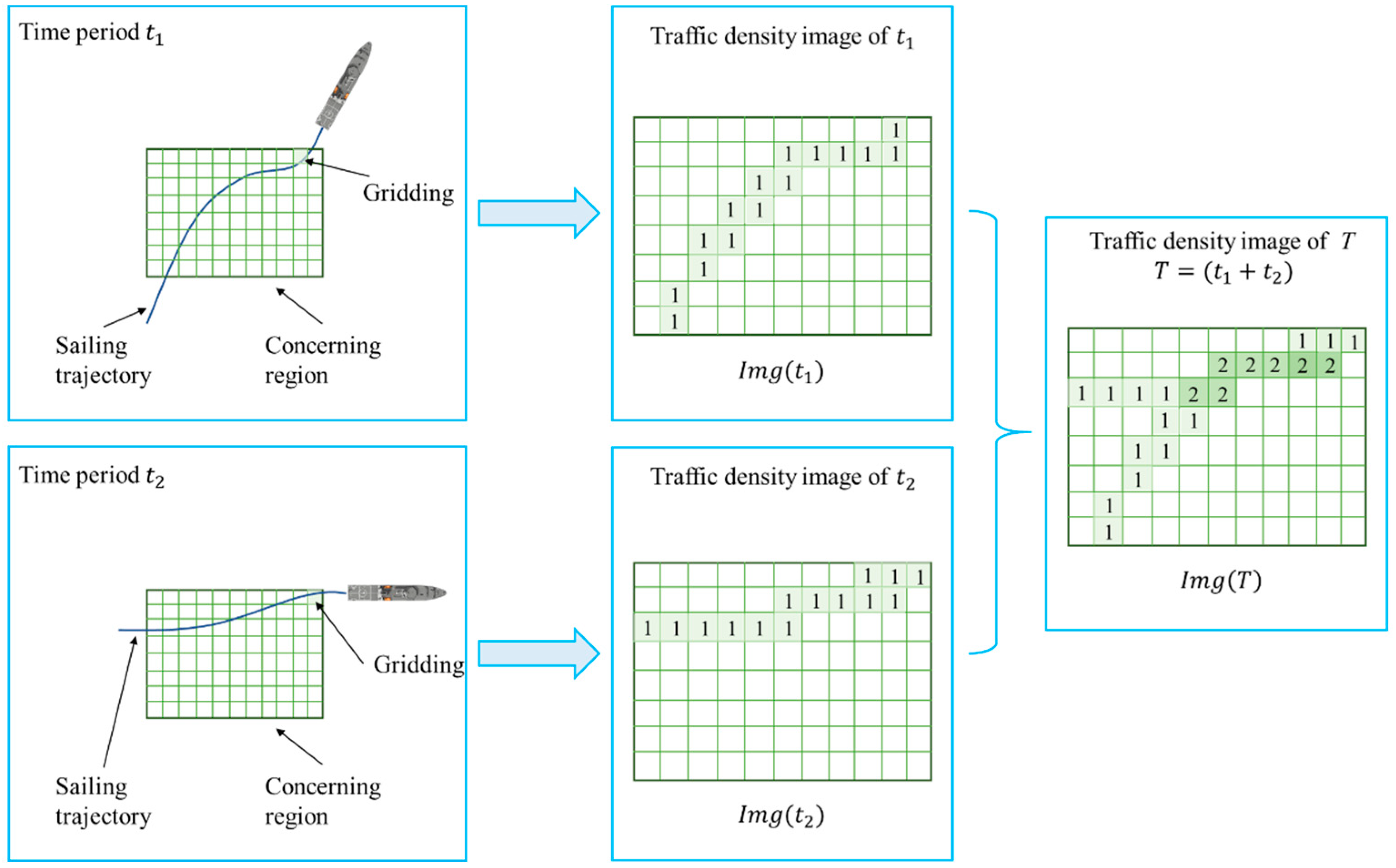
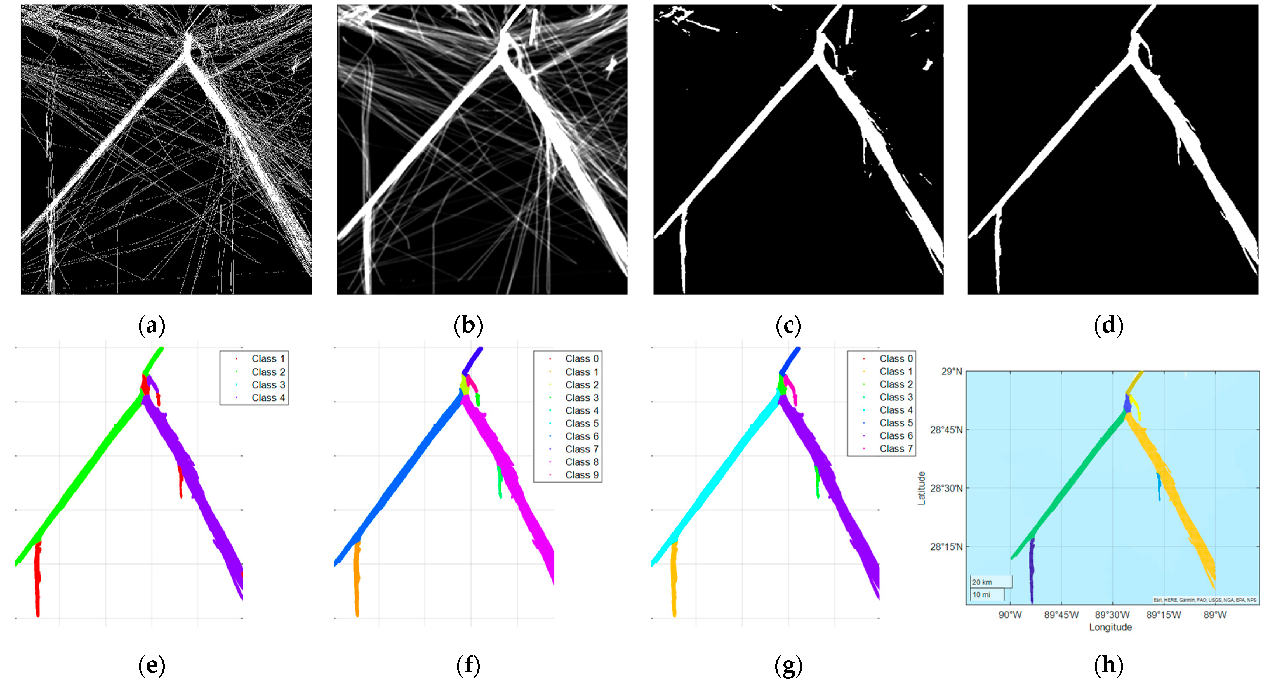
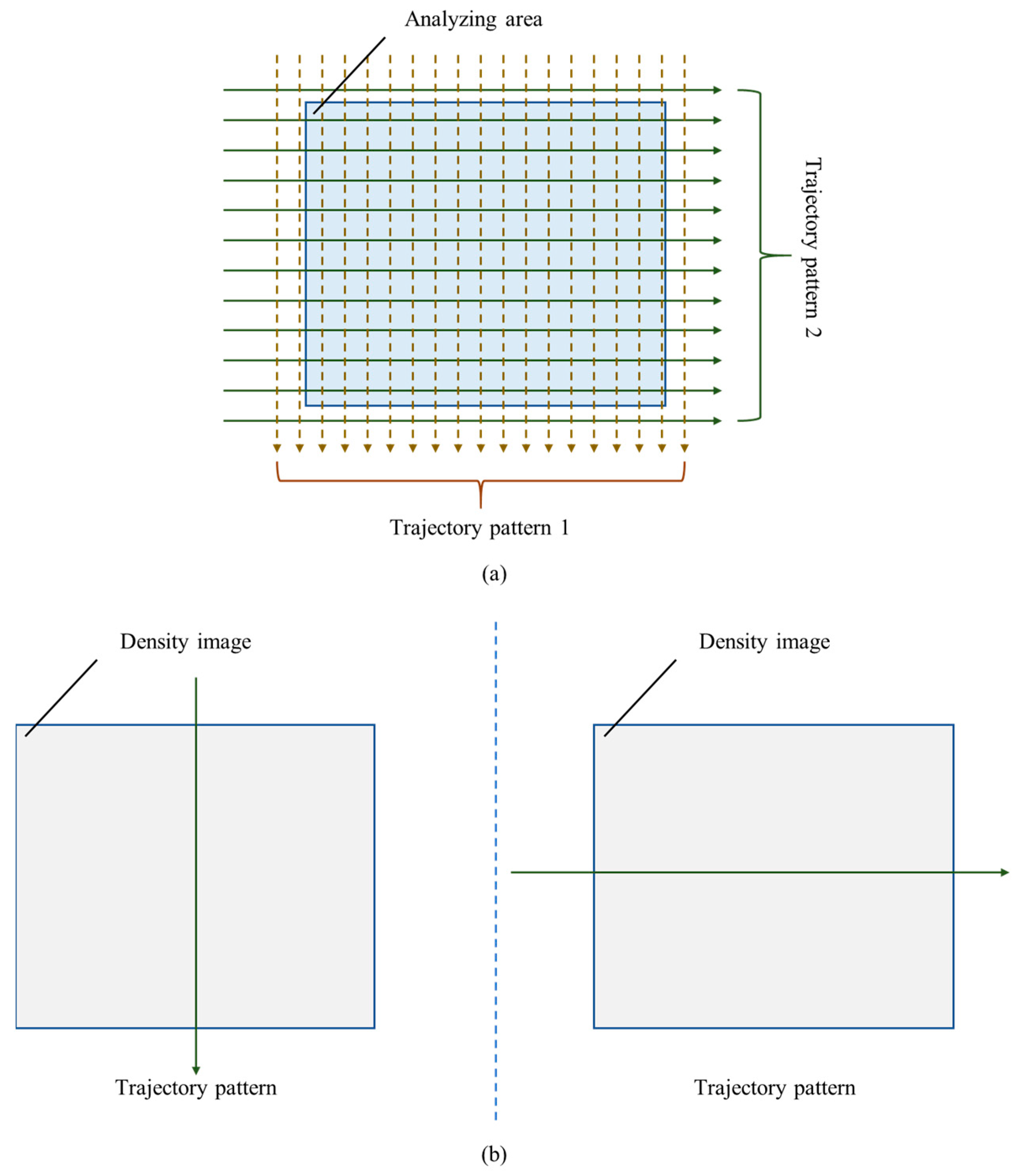
3.2. Construct Traffic Density Image

The traffic density image was constructed by counting the AIS points in each grid, and the pixel value was the number of AIS points. Traffic density is relatively stable and is widely used in trade analysis and ship flows [41]. For a certain region, the constructed traffic density image exhibits the following linear characteristics, as shown in Figure 2:

$$Img(T)={\displaystyle \sum _{i}Img(t_i)},T={\displaystyle \sum _i{t}_i}$$

(2)

where $Img(t)$ is the traffic density image of time period $t$.

Using Equation (2), traffic density images of different time periods can be directly added to obtain the traffic density image of the total period with a fixed dimension, which can effectively solve the curse of dimensionality. The construction process of the traffic density image is shown in Figure 2. In this study, a pixel of the traffic density image represented a 100 m × 100 m region (approximately 0.001° longitude and latitude). Note that the padding data are used to construct a traffic density image; for example, when we want to analyze a region of 28° N~29° N and 89° W~90° W, we need to construct a traffic density image with data of (28 − ∆)° N~(28 + ∆)° N and (89 − ∆)° W~(90 + ∆)° W, and the dimension of padding data depends on the variance of Gaussian filter.

After constructing a traffic density image, an image processing method can be used to analyze sea routes and make decisions.

3.3. Cluster Main Sea Routes

According to the construction process in Figure 2, the brightness of pixel in traffic density image is in direct proportion to the traffic density. The brighter regions indicate more ships sailing, which are more likely to be main sea routes, while the dark regions are less important for analyzing main sea routes. So, in image processing, the main sea routes are brighter regions in the traffic density image, whereas the others can be treated as image noise. First, we used a Gaussian filter to suppress minor sailing trajectories in a traffic density image, as shown in Figure 3a, by using Equation (3).

$$Im{g}_1=G_f(\sigma )\ast Im{g}_0$$

(3)

Here, $Im{g}_1$ is the filtered traffic density image obtained using the gaussian filter $G_f$ with a variance of $\sigma$, and $Im{g}_0$ is the original traffic density image. A filtered traffic density image is shown in Figure 3b.

Based on the concept of constant false alarm rate [42] (CFAR), the main sea routes were extracted using Equation (4):

$$R_L=\{x_L:x_L\ge T_b\},P(T_b)=\alpha$$

(4)

Here, $x_L$ is the pixel value of $Im{g}_1$; $T_b$ is the extraction threshold; $P$ is the empirical cumulative distribution function of $Im{g}_1$; and $\alpha$ is a significant level.

Note that the extracted region may also be the intersection region outside the main sea routes (Figure 3c); therefore, we performed morphological processing and connected component analysis to eliminate these regions.

$$A(x_L)\le A_0 \mathrm{OR} Ec(x_L)\le E{c}_0$$

(5)

Here, $x_L$ is the connected region of $R_L$, $A(x_L)$ and $Ec(x_L)$ is the area and eccentricity of region $x_L$, respectively, and $A_0$ and $E{c}_0$ is the threshold constant. We denote the processed traffic density image using Equation (5) as $Im{g}_M$.

Once we have all the main sea route regions in the traffic density image, as shown in Figure 3d, the next step is to cluster and segment them into different sailing patterns.

• Step 1: cluster regions based on sailing course

In the traffic density image, we can observe that the sailing course of the sea route can be reflected by textural features, indicating that sailing patterns can be classified using the textural features of traffic density images.

A Gabor filter was used to extract the textural features of the traffic density image. The Gabor filter is a linear bandpass filter that is widely used in image processing for edge detection, texture classification, feature extraction, and disparity estimation [43]. The Gabor feature $H_G$ is the sum of the response vectors for the same filter orientation obtained by convolving the image $Im{g}_M$ with the Gabor filter $\{g(x,y|\lambda ,\theta ,\psi ,\sigma ,\gamma )\}$:

$$\begin{array}{l}g(x,y|\lambda ,\theta ,\psi ,\sigma ,\gamma )=\exp (-\frac{{\tilde{x}}^2+{\gamma }^2{\tilde{y}}^2}{2{\sigma }^2})\exp \left[i\left(2\pi \frac{\tilde{x}}{\lambda }+\psi \right)\right],\\ \tilde{x}=x\cos \theta +y\sin \theta ,\tilde{y}=-x\sin \theta +y\cos \theta \end{array}$$

(6)

and using Equation (6), $H_G$ can be obtained in Equation (7),

$$\begin{array}{l}{H}_G=[h_g(1),\dots ,h_g(m)]\\ h_g(i)={\displaystyle \sum _{k}g(x,y|{\lambda }_k,{\theta }_i,\psi ,\sigma ,\gamma )\ast Im{g}_M}\end{array}$$

(7)

Here, $m$ is the dimension of orientations $\theta$.

We used the DBSCAN method to cluster pixels using the Gabor feature. The DBSCAN algorithm constructs the $\epsilon$-neighborhood of the data point as following Equation (8):

$$N_{\epsilon }(p)=\{q\in X^c|dist(p,q)\le \epsilon \}$$

(8)

where $dist$ is the distance function, we choose $L_2$ norm as distance function in our method.

The DBSCAN method uses the neighborhood density threshold $M_{\epsilon }$ to discover the clusters of the dataset that contains at least $M_{\epsilon }$ central points. These parameters can be chosen according to the max value of Gabor response. We note that the DBSCAN used in our method is to find the local features in density image, which is quite different in current clustering methods, that is, to cluster the vessel sailing routes.

• Step 2: check regions based on spatial location and density

After step 1, the sea routes with similar sailing courses are clustered in the same sailing pattern, as shown in Figure 3e. Subsequently, we add the position to the image feature and perform DBSCAN for each sailing pattern to achieve the sea routes isolated in space, as shown in Figure 3f. However, we observed that some adjacent regions exhibited over-segmentation, which can lead to inaccurate clustering results. We then checked these regions based on the spatial location and density of each sailing pattern to achieve more accurate segmentation.

We propose the following criterion to judge whether to merge adjacent sea routes:

$$MI={\displaystyle \prod _{i=1}^n{I}_i^{\frac{w_i}{n}}},MI\in [0,1]$$

(9)

In Equation (9), a larger value $MI$ indicates larger similarity between adjacent sea-routes. Here, $I_i\in [0,1]$ represents the normalized indicator generated by the characteristic of image, and $w_i$ is the weight of corresponding indicator.

In this study, three characteristics are used to calculate the similarity. They are the region distance indicator $I_1$, course similarity $I_2$, and density similarity $I_3$. The region distance indicator $I_1$ uses the maximum–minimum distance to calculate the spatial distance between two adjacent sea routes:

$$\begin{array}{l}{D}_1=\underset{x_i\in A_1}{\max }(\underset{y_j\in A_2}{\min }({\Vert x_i-y_j\Vert }_2))\\ I_1={(1+\exp (a_1(D_1-b_1)))}^{-1}\end{array}$$

(10)

where $A_1$ and $A_2$ are the adjacent sea route regions, $x_i$ and $y_j$ are the spatial coordinates of the pixels, and $a_1$ and $b_1$ are the parameters.

Course similarity $I_2$ uses the mean course of sea routes to prevent sudden course changes in one sea route:

$$\begin{array}{l}{D}_2={\Vert {\overline{\theta }}_1-{\overline{\theta }}_2\Vert }_1\\ {\overline{\theta }}_k={\theta }^T\frac{{\mu }_A(w^T{\overline{h}}_k)}{1^T\cdot {\mu }_A(w^T{\overline{h}}_k)}\\ I_2={(1+\exp (a_2(D_2-b_2)))}^{-1}\end{array}$$

(11)

where $\theta$ is the orientation of the Gabor filter, $m$ is the dimension of $\theta$, ${\overline{h}}_i$ is the mean Gabor feature vector of the sea route region $A_k$, $a_2$ and $b_3$ are the parameters, and ${\mu }_A(w^T{\overline{h}}_i)=[{}^1\mu _A(w^T{\overline{h}}_i),\dots ,{}^m\mu _A(w^T{\overline{h}}_i)]$ is the fuzzy membership vector. The fuzzy membership functions use the following exponential functions:

$${}^n\mu _A(w^T{\overline{h}}_k)=e^{-\alpha {(w^T{\overline{h}}_k-\beta )}^2},n=1,\dots ,m$$

(12)

Here, $\alpha ,\beta$ are the shape parameters of fuzzy membership function.

The density similarity $I_3$ use the mean traffic density of sea routes to imbalance density in one sea route:

$$\begin{array}{l}{D}_3=\frac{{\Vert t_1-t_2\Vert }_1}{\overline{\sigma }}\\ I_3={(1+\exp (a_3(D_3-b_3)))}^{-1}\end{array}$$

(13)

where $t_i$ is the mean traffic density (grayscale) of sea route region $A_i$; $\overline{\sigma }$ is the mean standard deviation of grayscale of sea route regions; $a_3$ and $b_3$ are the parameters.

Using Equations (10)–(13), by choosing the merging threshold $M{I}_0$, we can merge these adjacent sea routes with $MI>M{I}_0$, and the results are shown in Figure 3g,h. The entire process is shown in Figure 3.

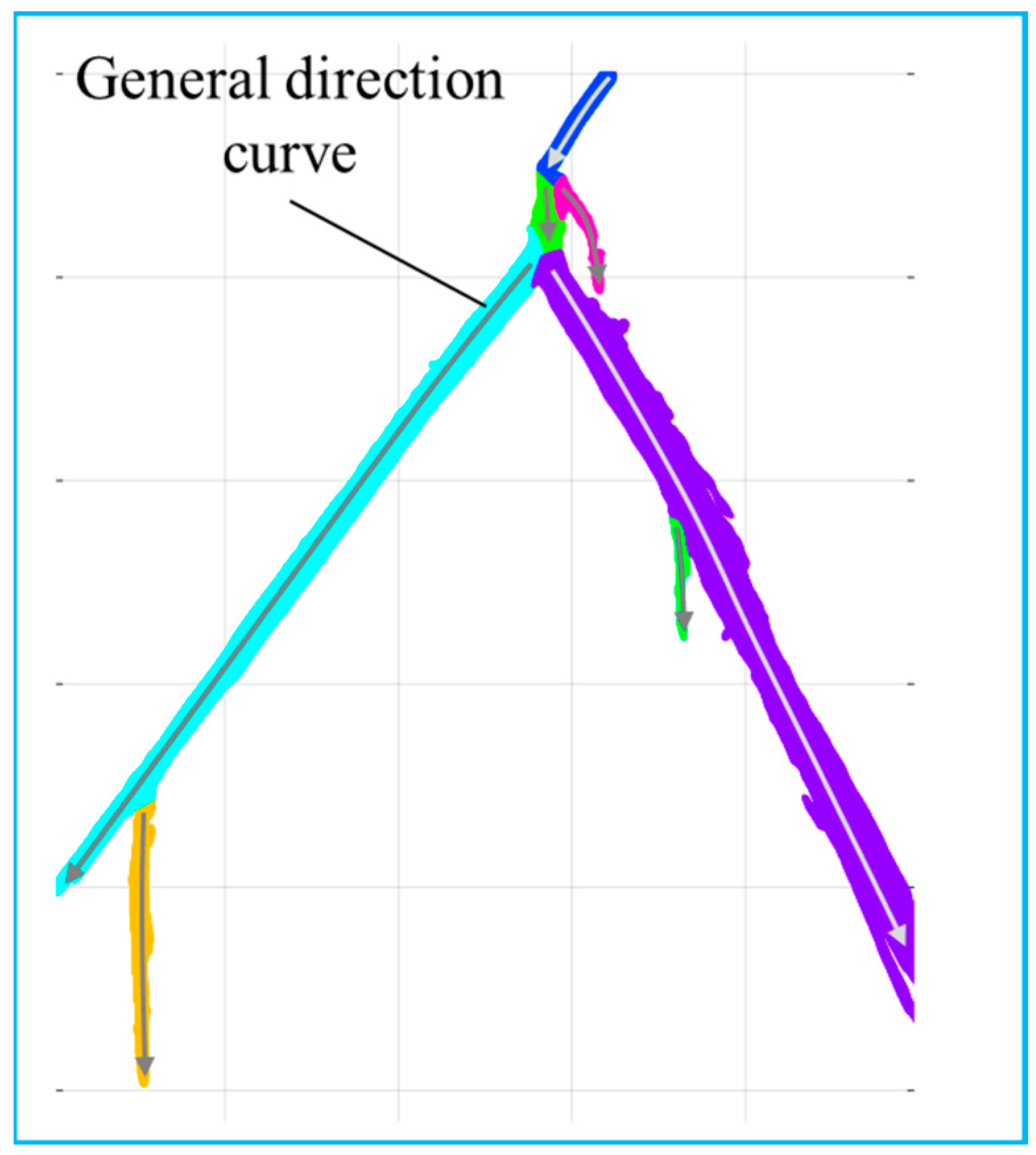
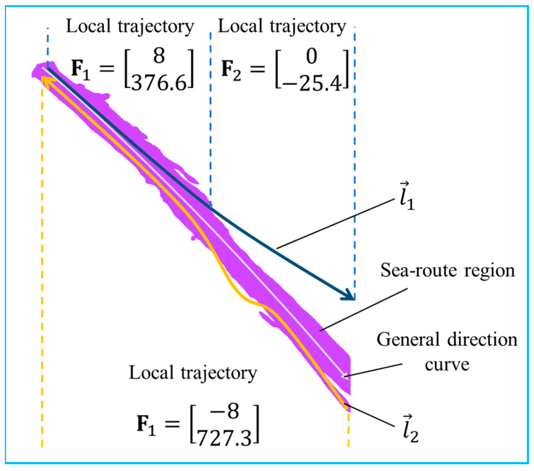
3.4. Identify the Sailing Trajectory

We can now use the main sea routes to identify the given sailing trajectories. We first define the general direction curve of each sea route region based on the direction of the representative AIS trajectory, as shown in Figure 4. The general curve was calculated according to the main centerline of the sea route region using the image skeleton. A representative AIS trajectory is defined as follows:

• The representative AIS trajectory (or trajectory segmentation) of a sea route region should belong to the corresponding sea route region.
• The Hausdorff distance [44] between the representative AIS trajectory and the general direction curve should be less than a given threshold.

Note that the representative AIS trajectory is not unique, and only the general direction is used to classify the AIS trajectories.

Let $\overrightarrow{l}=[x_1,\dots ,x_n]$ denote a certain AIS trajectory, $x_i$ be the chronological ship position, and $\left\{A_i\right\}$ denote the segmented sea route regions; subsequently, we code $\overrightarrow{l}$ as the following feature matrix:

$$F(\overrightarrow{l})=\left[\begin{array}{c}{F}_1\\ F_2\end{array}\right]=\left[\begin{array}{ccc}\pm k_1& \dots & \pm k_m\\ L_1& \dots & L_m\end{array}\right]$$

(14)

where $F_1$ is the pattern feature vector, $F_2$ is the quantity feature vector, and $k_i$ is the pattern of local trajectory. When the ship course has an acute angle between the general direction curve, we choose $+k_i$; otherwise, we choose $-k_i$, and $L_i$ is the length of the local trajectory that belongs to a certain pattern.

The coding process of Equation (14) is shown in Figure 5, where local trajectories with the same pattern are merged when the merged trajectories have over 70% of the length belonging to the pattern. Note that when the local trajectory does not belong to any pattern, $k_i$ is chosen as 0, and $L_i$ is chosen as the mean course relative to the x-direction.

We used the Smith–Waterman algorithm [45] to determine the most suitable local match between the pattern feature vectors of AIS trajectories ${\overrightarrow{l}}_1$ and ${\overrightarrow{l}}_2$, and the scoring criteria are defined as follows:

$$s(a_i,b_i)=\{\begin{array}{l}+1,\hspace{1em}\hspace{1em}{a}_i=b_j\\ -1,\hspace{1em}\hspace{1em}{a}_i\ne b_j \mathrm{and} a_i \& b_j=0\\ -2,\hspace{1em}\hspace{1em}{a}_i\ne b_j \mathrm{and} a_i \& b_j\ne 0\end{array}$$

(15)

where $a_i$ and $b_j$ represents the i-th element and j-th element of $F_1$(${\overrightarrow{l}}_1$) and $F_1$(${\overrightarrow{l}}_2$), respectively, and $F_1^{\ast }$ and $F_2^{\ast }$ denotes the most suitable local match of ${\overrightarrow{l}}_1$ and ${\overrightarrow{l}}_2$.

Using Equation (15), the distance between AIS trajectories ${\overrightarrow{l}}_1$ and ${\overrightarrow{l}}_2$ is calculated using Equation (16):

$$\begin{array}{cc}\hfill DL({\overrightarrow{l}}_1,{\overrightarrow{l}}_2)& ={\displaystyle \sum _k{\alpha }_1{y}_k\frac{\left|L_{1,k}-L_{2,k}\right|}{L_{1,k}+L_{2,k}}}+{\displaystyle \sum _i{\alpha }_2{y}_i\frac{\left|L_{1,i}-L_{2,i}\right|}{\left|L_{1,i}\right|+\left|L_{2,i}\right|}}\hfill \\ & +{\displaystyle \sum _j{\alpha }_3{y}_j}+\frac{\max (L(F_1),L(F_2))}{L(F_1^{\ast })}\hfill \end{array}$$

(16)

where $y_k,y_i,y_j$ are the sign functions representing the different conditions of local match, when $F_1^{\ast }(k)=F_2^{\ast }(k)\ne 0$, $y_k=1$; when $F_1^{\ast }(k)=F_2^{\ast }(k)=0$, $y_i=1$; when $F_1^{\ast }(k)\ne F_2^{\ast }(k)$, $y_j=1$; otherwise, $y_k,y_i,y_j=0$; ${\alpha }_1,{\alpha }_2,{\alpha }_3$ are the weighted factors; and $L(F_1),L(F_2),L(F_1^{\ast })$ represent the length of $F_1,F_2,F_1^{\ast }$, respectively.

Given a threshold $T{h}_0$, we can cluster the AIS trajectories using the between-class distance $DL\le T{h}_0$ as a single sailing cluster. Therefore, the efficient compression of AIS trajectories is accomplished. To solve the problem of dimensionality further, we can use the following Algorithm 1 to construct reference patterns:

Algorithm 1: Reference patterns of main sea routes

Input: Main sea routes ${\mathit{I}\mathit{m}}_{\mathit{s}\mathit{r}}$; Distance matrix of sea routes ${\mathit{D}\mathit{i}\mathit{s}}_{\mathit{s}\mathit{r}}$. Output: Reference patterns ${\mathit{F}}_{\mathit{r}\mathit{e}\mathit{f}}$.

1. Let $k=1$; 2. Choose $k$-th sea route region, let $A_1=k$ and add $A_1$ to ${\mathit{F}}_{\mathit{r}\mathit{e}\mathit{f}}$; 3. Choose sea route regions with the minimum distance between $k$-th sea route region as $\left\{a_m\right\}$;  3.1 When $\left\{a_m\right\}\ne \varnothing$, let $i=1$, else, go to step 4;  3.2 Let $A_2=\{A_1,a_i\}$ and add $A_2$ to ${\mathit{F}}_{\mathit{r}\mathit{e}\mathit{f}}$;  3.3 Choose sea route regions except for $A_2$ with the minimum distance between $a_i$-th sea route region as $\left\{b_n\right\}$;  3.4 When $\left\{b_n\right\}\ne \varnothing$, use the recursive method to analyze the rest of sea route regions until $\varnothing$ is obtained, else, go to step 3.5;  3.5 Let $i=i+1$, go to step 3.2; 4. Let $k=k+1$, go to step 2; 5. For each sequence in ${\mathit{F}}_{\mathit{r}\mathit{e}\mathit{f}}$, successively add 0 to the sequence from beginning to end, obtain ${\mathit{F}}_{\mathit{r}\mathit{e}\mathit{f}}^{\prime }$; 6. Output ${\mathit{F}}_{\mathit{r}\mathit{e}\mathit{f}}=\{{\mathit{F}}_{\mathit{r}\mathit{e}\mathit{f}},{\mathit{F}}_{\mathit{r}\mathit{e}\mathit{f}}^{\prime }\}$;

Note that if some main vessel sailing routes are known as priors, they can be directly added to the reference patterns ${\mathit{F}}_{\mathit{r}\mathit{e}\mathit{f}}$ and replace similar patterns in Algorithm 1. The reference patterns indicate all potential clusters for analyzing the AIS data, which determines the maximum number of clusters in the proposed method.

The contributions of this study can be summarized as follows:

• The proposed method uses the traffic density image to transform the clustering problem of complex AIS trajectories into an image processing problem, and the traffic density images of different time periods can be directly added together to obtain the traffic density image of the total period with a fixed dimension, which can effectively solve the curse of dimensionality.
• The proposed method only calculates the similarity between the given AIS trajectory and the constructed reference patterns. The similarity between trajectories is not required in this method, which significantly shortens the clustering operation time for large-scale AIS data compared to commonly used density-based methods.
• The proposed method can effectively consider local and global features of trajectories and deal with complex AIS data with different vessel densities and sailing patterns. In addition, the noise data can also be eliminated.

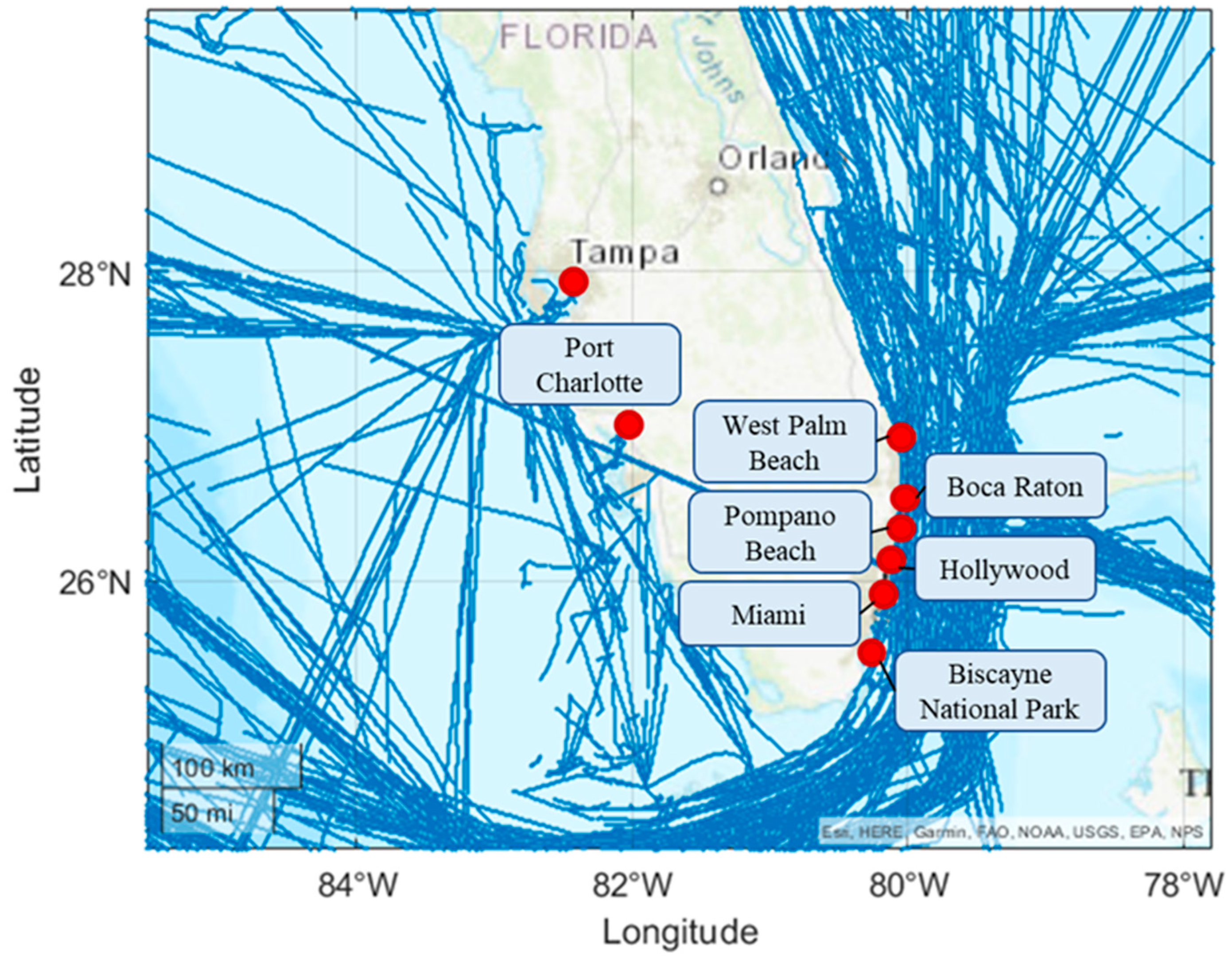
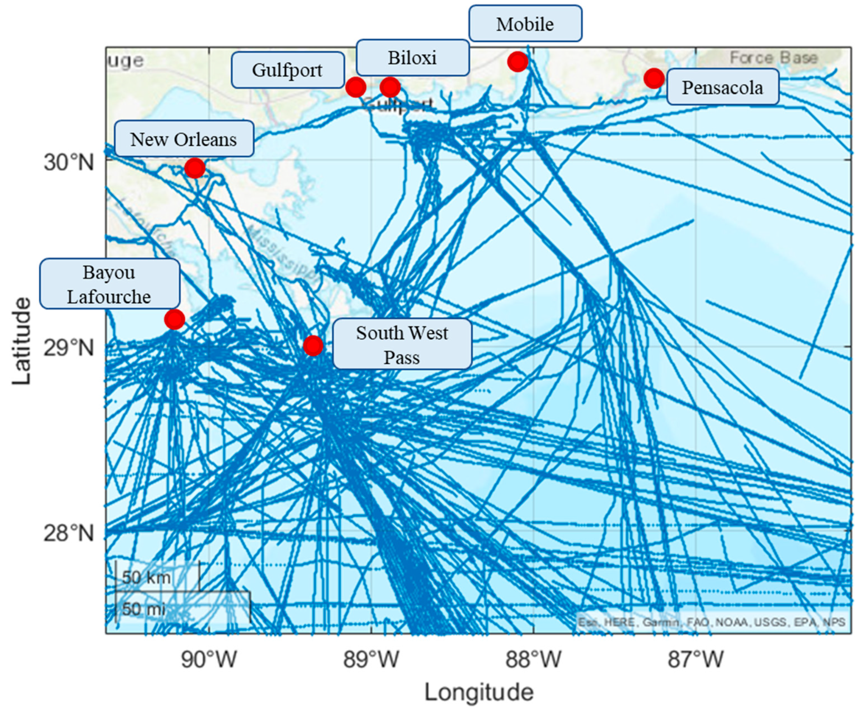
4. Case Studies and Results

In this section, we verify the effectiveness of the proposed method using the AIS data of U.S. coastal waters in January 2022 from the Marine Cadaster, South American Sea (shown in Figure 6). Here, we choose the background of Gulf of Mexico for the following reason: First, the chosen region includes some big port cities like Boca Raton, Hollywood, and Miami, which makes the AIS data complex and large. Second, this gulf area includes various situations like coastal waters and straits, which can better verify the robustness and adaptability of the proposed method. The case studies were divided into a performance comparison experiment and a time–space domain covering experiment.

Performance comparison experiment: Compare the proposed method with several other clustering methods to verify the effectiveness and advancement of the proposed method.

Time–space domain covering experiment: The experiment used different AIS data of regions to show the effectiveness and advancement of the proposed method, which can be difficult to solve using the contrastive methods presented.

All experiments were performed on a computer running 64-bit Windows 11 with a 3.20 GHz AMD Ryzen 7 6800H with a Radeon Graphics CPU and 16 GB of memory. The methods were achieved in Pycharm and basic algorithms were realized using Scikit-Learn, which is a Python library that provides simple and efficient tools for predictive data analysis. The parameters for our method were chosen as follows:

We choose orientations $\theta =[0,\frac{\pi }{6},\frac{\pi }{3},\frac{\pi }{2},\frac{2\pi }{3},\frac{5\pi }{6}]$ and wavelength $\lambda =[2,4,8]$ of the Gabor filter; the DBSCAN parameters in our case can be chosen as $\epsilon =5,M_{\epsilon }=5$.

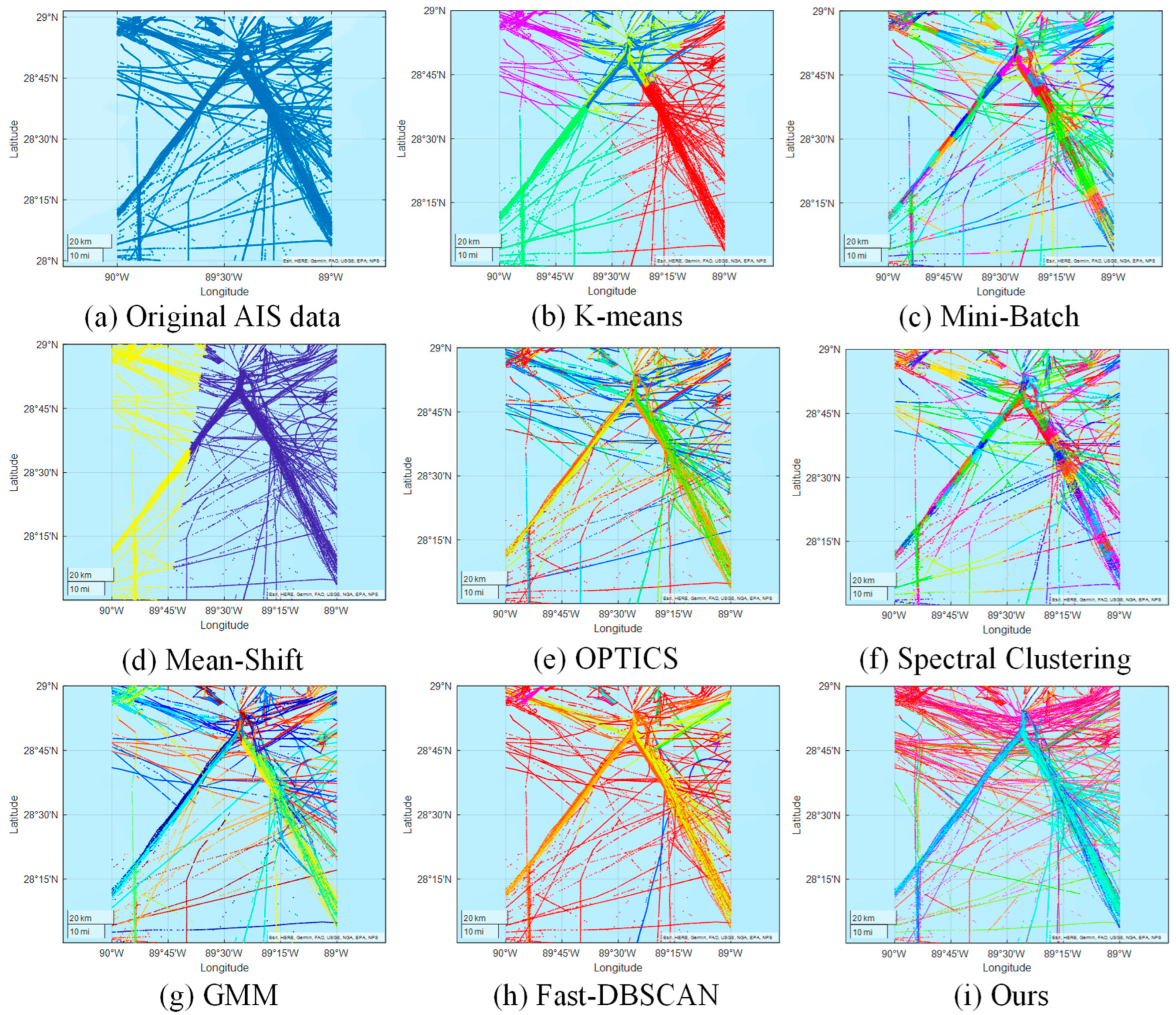
4.1. Performance Comparison Experiment

First, we demonstrated the comparative clustering performance of the proposed method and a group of classical clustering methods. We used the AIS data from 1 January 2022 to 7 January 2022, in a region of 28° N~29° N and 89° W~90° W, Gulf of Mexico, with a total of 30,015 valid AIS vessel trajectories. Seven representative clustering methods were compared. We mainly used the silhouette coefficient, Calinski–Harabasz index, Davies–Bouldin index, adjusted Rand score, adjusted mutual information score, V-measure, and Mallows score to evaluate the performance of the clustering results [46]. The total computing time was also analyzed. The clustering results of the performance comparison experiments are shown in Figure 7.

Figure 7a shows the original distribution of the AIS data, and Figure 7b–i shows the clustering results of different clustering methods, where each color represents a clustering pattern. The original distribution of the AIS data is spatially heterogeneous, and the trajectories are noisy and often intersected, which causes difficulty in clustering the AIS data of the analyzed region. The corresponding performance characteristics were calculated to compare the clustering methods, as listed in

Table 1. Clustering performance characteristics of eight comparative clustering methods.

Methods	Performance
	Clusters	Silhouette Coefficient	Calinski–Harabasz Index	Davies–Bouldin Index	Adjusted Rand Score	Adjusted Mutual Information	V-Measure	Mallows Score	Time Cost
k-means [48] (Affandi et al., 2020)	6	0.4571	26,987.0236	1.0514	0.2300	0.3798	0.3798	0.5354	12.7614 s
Minibatch [49] (Tang and Fong, 2018)	240	0.3815	17,812.3450	0.8272	0.2947	0.4732	0.4732	0.5125	37.5809 s
Mean shift [50] (Chen et al., 2017)	2	0.5666	18,505.3470	1.1534	0.1876	0.2715	0.2715	0.5461	786.6635 s
OPTICS [51] (Rong et al., 2022)	240	−0.4389	1072.4056	1.8995	0.0363	0.2293	0.2293	0.4897	524.7466 s
Spectral clustering [25] (Gao and Shi, 2020)	240	0.3768	4467.0755	1.3781	0.1959	0.4987	0.4987	0.5095	170.5076 s
Gaussian mixture [52] (Yu et al., 2018)	49	−0.0381	3469.1872	2.5320	0.1255	0.4110	0.4110	0.5032	600.3050 s
Fast-DBSCAN [47] (Chen et al., 2023)	203	−0.2005	1705.9510	1.5039	0.3139	0.3880	0.3879	0.5081	309.6005 s
Ours	52	−0.8649	783.2227	24.9302	0.7638	0.8874	0.8875	0.8123	235.7099 s

. Note that the cluster number is not a parameter in the proposed method; the reference patterns indicate all the potential clusters for analyzing the AIS data, and this is the maximum number of clusters in the proposed method. By choosing clusters with large densities (using the quantile or KDE method), the main sailing routes of the analyzed region can finally be acquired. The cluster number of the comparative clustering methods was chosen following the practice in [47].

From Table 1, it can be observed that the k-means method has the fastest calculation speed and is suitable for largescale datasets. It costs about 12.7614 s to accomplish the cluster including determining the number of clusters. However, the conventional k-means method has poor processing ability for non-spherical clusters and attends to convex clustering results. In addition, the k-means method is easily affected by the selection of initial cluster centers and may assign noise data or outliers to incorrect clusters. These disadvantages lead to poor performance for the analyzed AIS data (shown in Figure 7b), and low clustering performance characteristics like adjusted mutual information.

Mean shift clustering is a density-based nonparametric clustering algorithm whose basic idea is to identify clusters in data by finding the location of the highest density of data points. The mean shift does not need to specify the number of clusters and has a positive effect on clusters with complex shapes. However, the mean shift has relatively high computational complexity and is sensitive to the selection of initial parameters, as shown in Figure 7d. Using the conventional bandwidth detection method, we can only have two clusters, which is not accurate.

Both spectral clustering and minibatch methods were developed to achieve the minimum distance from all trajectory points to the set cluster. Because the original distribution of the AIS data was spatially heterogeneous, the distance distribution to each cluster was also different. These factors led to an unsatisfactory clustering performance, as shown in Figure 7c,f.

Both OPTICS and fast-DBSCAN methods use a density-based clustering algorithm that can efficiently discover clusters of arbitrary shapes and process noisy data. Compared to traditional DBSCAN, OPTICS and fast-DBSCAN can automatically determine the number of clusters and are easy to analyze and visualize. However, these algorithms may have a poor clustering effect on datasets with large density differences, and the overall features of the trajectories were not used.

In general, the proposed method exhibited the best clustering performance with regard to rapidity and accuracy. All the adjusted rand scores, adjusted mutual information scores, V-measures, and Mallows scores were better than the others and improved by over 50%. Meanwhile, its computing time is also acceptable at approximately 235.71 s, which is faster than other density-based methods. The detailed performance characteristics are listed in Table 1.

Choosing the clusters with large density, the main sailing routes of the analyzed region acquired by the proposed method are shown in Figure 8, and all the potential sailing routes are manually annotated, as shown in Figure 9.

The proposed TDIBC method can effectively acquire the correct sailing routes and eliminate outlier trajectory noise in complex AIS data without using prior knowledge. In addition, the proposed method can deal with intersecting trajectories by considering both local and global features of the trajectories. The results prove that the proposed method has a strong ability to cluster AIS data with a complex distribution and has good application potential for analyzing real big AIS data.

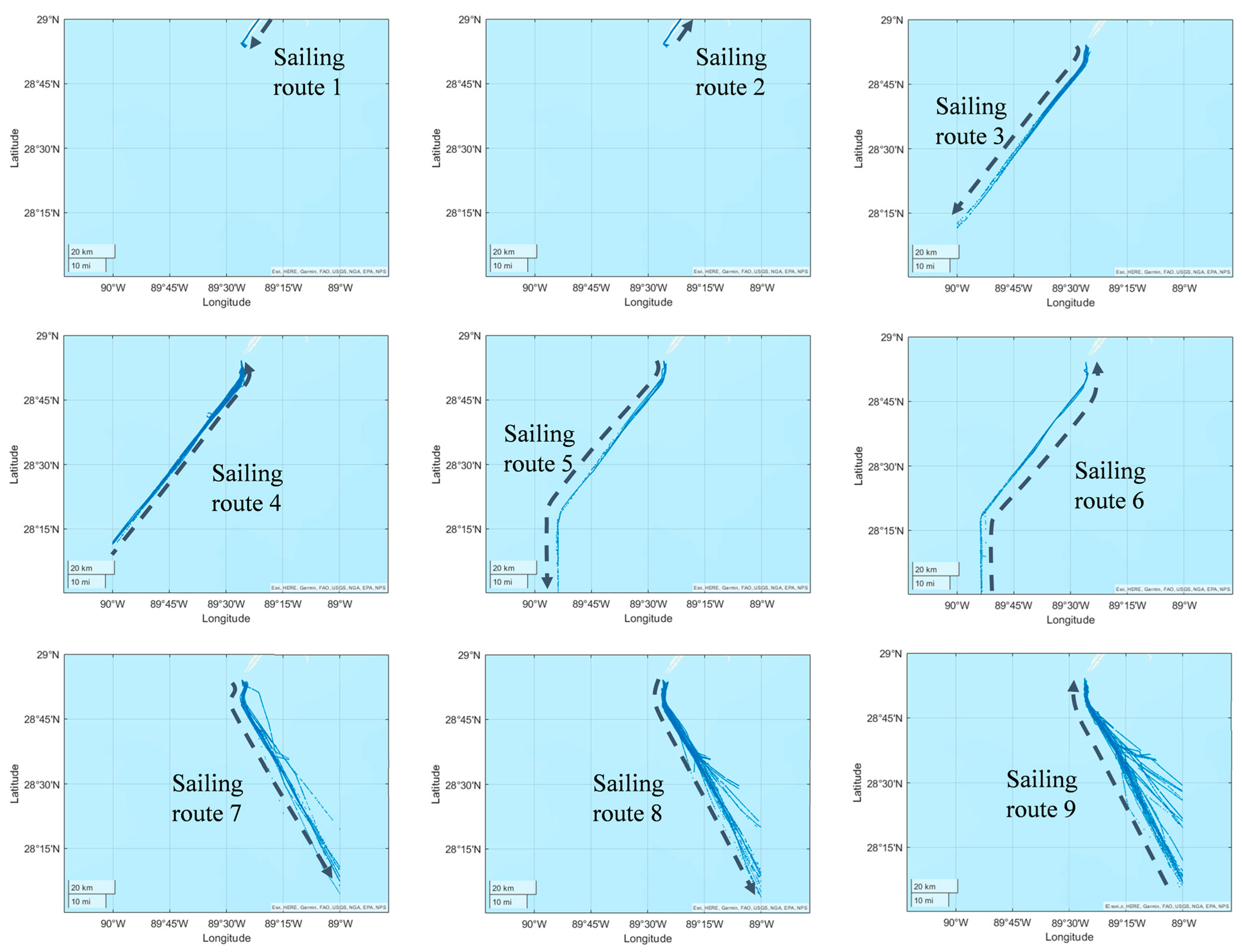
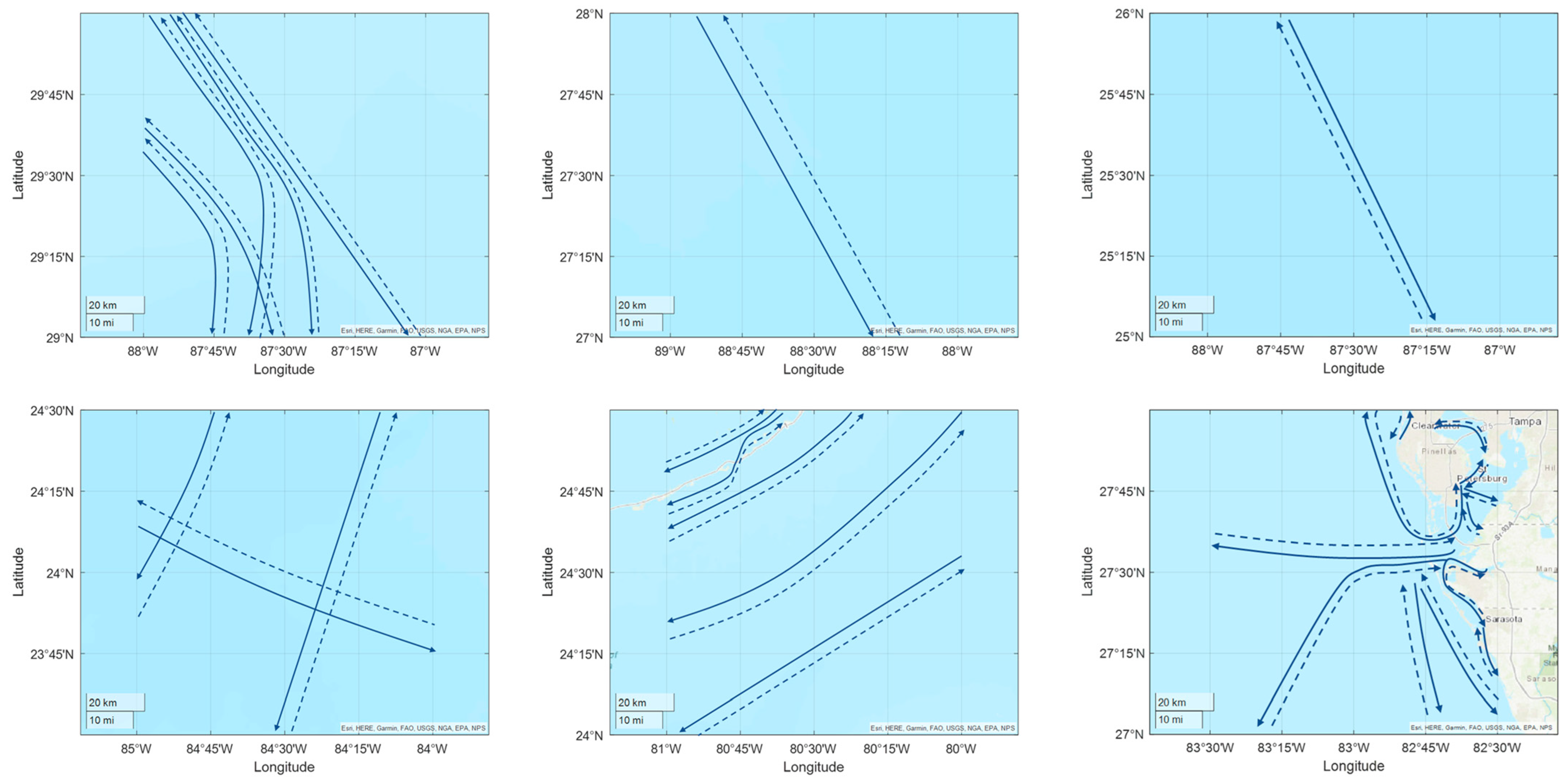
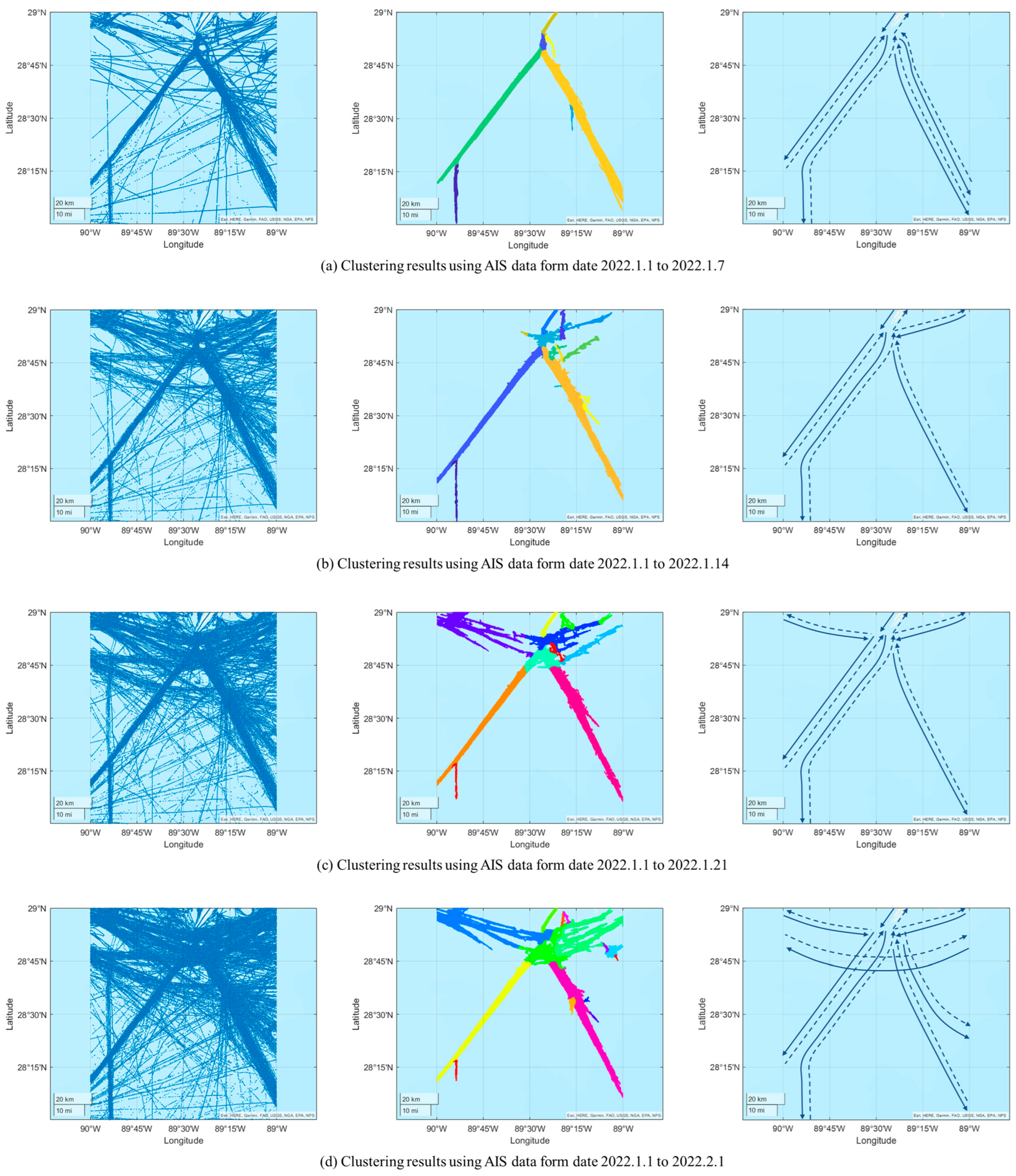
4.2. Time–Space Domain Covering Experiment

In this experiment, we demonstrated the stable performance and the time–space applicability of our method. We first used the AIS data from 1 January 2022 to 7 January 2022 in the following four representative regions: 1. 29° N~30° N and 87° W~88° W, 2. 27° N~28° N and 88° W~89° W, 3. 23.5° N~24.5° N and 84° W~85° W, 4. 24° N~25° N and 80° W~81° W, 25° N~26° N and 87° W~88° W, 27° N~28° N and 82.5° W~83.5° W, Gulf of Mexico. The analyzed regions cover different vessel densities and various sailing patterns, as shown in Figure 10.

The experimental results are shown in Figure 11, Figure 12 and Figure 13. Figure 11 shows the original distribution of the AIS data, Figure 12 shows the corresponding clustering results, and Figure 13 shows the acquired sailing patterns for identifying the AIS trajectories.

As shown in Figure 12 and Figure 13, the proposed method can effectively manage complex AIS data with different vessel densities and sailing patterns. The main sea routes can be extracted regardless of whether the trajectories are isolated or intersecting. By combining the results in Section 4.1, we observe that the proposed TDIBC method applies to various situations, including high seas, coastal waters, and straits, which demonstrates the robustness of the proposed method to the density distribution of data. We can also observe that, although large outliers or isolated points exist, the proposed method can effectively eliminate trajectory noise due to the use of image filters and statistics-based global density information. Based on the above results, the proposed method can effectively acquire reasonable sailing patterns for each analyzed region, and the AIS trajectories can be easily identified and clustered.

These experimental results demonstrate that our method is suitable for clustering largescale spatial AIS data. Furthermore, we demonstrated the stable performance and efficiency of the proposed method in the time domain. For contrastive analysis, we used AIS data from date 1 January 2022 to 1 February 2022 in a region of 28° N–29° N and 89° W–90° W, Gulf of Mexico, with a total of 293,868 valid AIS vessel trajectories.

The experimental results are shown in Figure 14. Figure 14a–d shows the clustering results of the proposed method using the AIS data from 1 January 2022 to 7 January 2022 (total of 30,015 valid AIS vessel trajectories), 1 January 2022 to 14 January 2022 (total of 131,520 valid AIS vessel trajectories), 1 January 2022 to 21 January 2022 (total of 196,811 valid AIS vessel trajectories), and 1 January 2022 to 1 February 2022 (total of 293,868 valid AIS vessel trajectories), respectively. The first column shows the original distribution of the AIS data, the second column shows the clustering results of the sea route regions, and the third column shows the acquired sailing patterns.

As shown in Figure 14, although the amount of AIS data changes significantly, the main sea route regions extracted using the proposed method are relatively stable, and this characteristic provides stable performance and the time–space applicability of the proposed method. As shown in Figure 14a, similar sailing patterns are over-segmented, and in Figure 14b–d, the over-segmented sailing patterns are classified as the same pattern. Comparing the acquired sailing patterns, we also observed that the acquired sailing patterns were more accurate when more AIS data were used to extract the main sea route regions. The time cost of these timescale AIS data using different clustering methods is listed in

Table 2. Time cost of eight comparative clustering methods in different timescale AIS data.

Methods	Time Cost
	AIS Data from 1 January to 7 January	AIS Data from 1 January to 14 January	AIS Data from 1 January to 21 January	AIS Data from 1 January to 1 February
k-means (Affandi et al., 2020 [48])	12.7614 s	13.0473 s	16.9655 s	26.7114 s
Minibatch (Tang and Fong, 2018 [49])	6.9864 s	8.6478 s	12.5502 s	16.8571 s
Mean shift (Chen et al., 2017 [50])	786.6635 s	5377.7543 s	9728.5147 s	15,910.2940 s
OPTICS (Rong et al., 2022 [51])	524.7466 s	765.9809 s	2688.7135 s	9731.3116 s
Spectral clustering (Gao and Shi, 2020 [25])	170.5076 s	/	/	/
Gaussian mixture (Yu et al., 2018 [52])	600.3050 s	909.2754 s	1432.8670 s	1760.0464 s
Fast-DBSCAN (Chen et al., 2023 [47])	309.6005 s	378.3306 s	1317.4696 s	4476.4033 s
Ours	235.7099 s	305.6329 s	427.8843 s	584.1705 s

; the blank data in Table 2 indicate that the method runs out of memory (over 15.2 GB in our environment).

From Table 2, it can be concluded that the calculation time of our method tends toward a stable value because of the relatively stable performance of the acquired main sea route regions and sailing patterns. Because our method only calculates the similarity between the given AIS trajectory and constructed reference patterns, the algorithmic time complexity of our method is approximately O(N_data · N_rp), where $N_{data}$ is the size of the AIS dataset and $N_{rp}$ is the size of the reference patterns. The advantage of the proposed method in terms of efficiency is more evident for clustering more AIS data than for density-based methods. In addition, the size of the array and memory used is limited in our method; therefore, the out-of-memory problem can always be avoided. These experimental results demonstrate that the proposed method is suitable for the clustering requirements of big AIS data.

5. Discussion

In this study, a method for efficiently clustering and analyzing vessel sailing routes from AIS data using traffic density images is proposed to meet the clustering requirements of big AIS data. The proposed method constructs a traffic density image of the AIS data, which transforms the clustering problem of AIS trajectories into an image-processing problem. Certain observations from the results are discussed below.

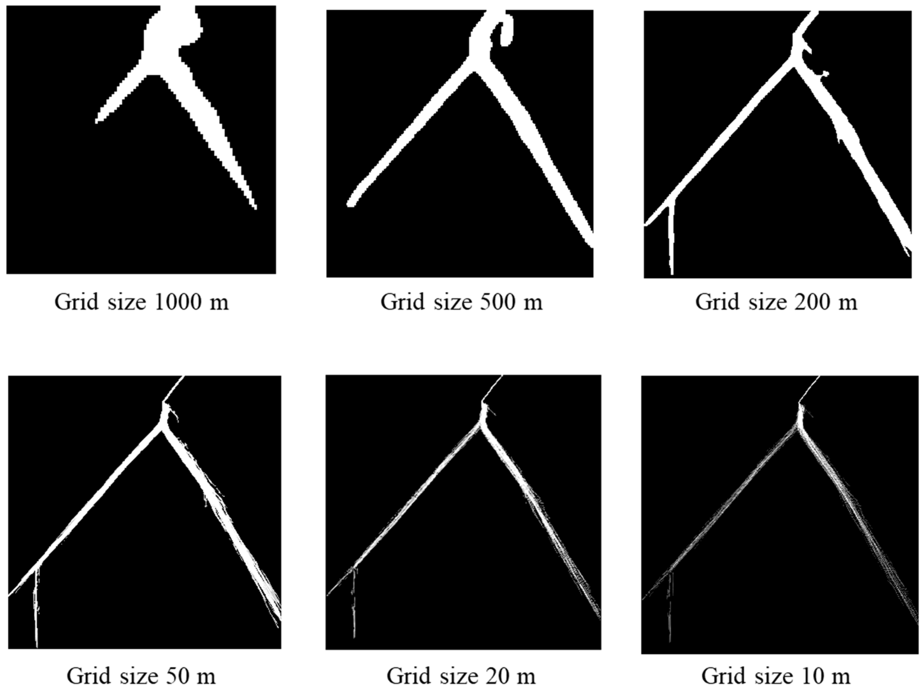
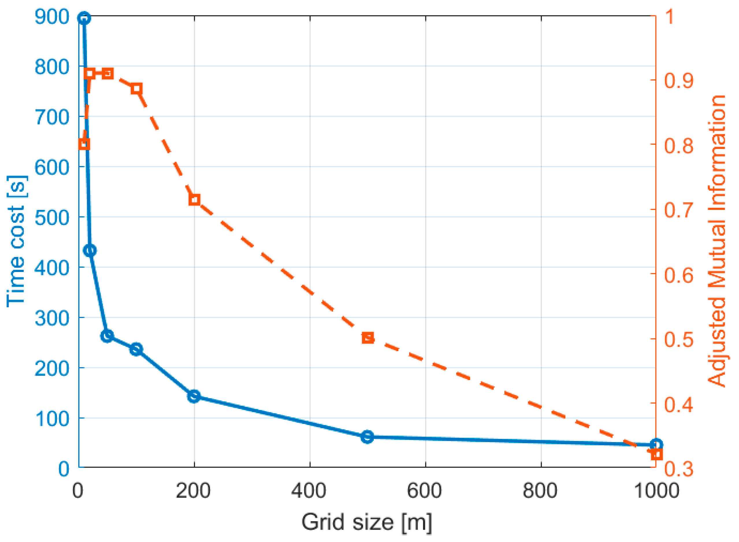
5.1. Parameter Setting

In general, two types of parameters influence the clustering performance of our method. One is the orientation $\theta$ and the wavelength $\lambda$ of the Gabor filter, and the other is the grid size.

The $\theta$ and $\lambda$ of Gabor filter influences the clustering result of main sea routes, and the strongest resolution of sailing direction appears on the corresponding $\theta$. When $\theta$ is chosen as $[0,\frac{\pi }{6},\frac{\pi }{3},\frac{\pi }{2},\frac{2\pi }{3},\frac{5\pi }{6}]$, we can effectively distinguish the sailing pattern every 30 degrees, and the resolution of sailing direction is 15 degrees, which means the mean absolute difference of sailing direction within 15 degrees is classified into one sailing pattern. The $\lambda$ influences the concerns of local features in the density image, and it should be larger than 2 and less than the hypotenuse length of the density image. Therefore, the parameters of Gabor filter are relatively robust to the constructed density image.

The efficiency of a clustering method is mostly dependent on the density of the image. The grid size influences the accuracy and efficiency. The smaller the grid size, the more explicit the segmentation of route regions, and a smaller grid size leads to a larger density image, which decreases the efficiency. Using the case presented in Section 4.1, we next demonstrate the influence of grid size. We chose the grid size as 10 m (approximately 0.0001°), 20 m (approximately 0.0002°), 50 m (approximately 0.005°), 200 m (approximately 0.002°), 500 m (approximately 0.005°), and 1000 m (approximately 0.01°), respectively. The extracted main sea routes are shown in Figure 15.

The clustering performance caused by grid size is shown in Figure 16.

We can observe that the time cost significantly increases when the grid size is less than 50 m because the size of the density image is inversely proportional to the square of the grid size, and the memory cost is proportional to the square of the grid size. The adjusted mutual information of the clustering results decreases significantly when the grid size exceeds 100 m. Clustered sea routes are less reasonable because more local features are lost owing to larger grid sizes. The adjusted mutual information of the clustering results also decreases when the grid size is 10 m because excessive concern for local features leads to over-segmentation of route regions. Therefore, it is ideal to have a grid size ranging from 50 to 100 m, and the accuracy and efficiency can be balanced well.

The influence of time period can be shown in Section 4.2; since empirical distribution can better approximate to real distribution when more data are used, we find the time period of data is suitable to be chosen at larger than one week. The influence of spatial scope is similar to that of the grid size, the lower bound depends on the concerning area, and the upper bound depends on the system memory; in our case, the image size should more than 500 × 500 and less than 10,000 × 10,000.

5.2. Practical Implications

The practical implications of the results are discussed as follows:

First, the accuracy can be improved by using more AIS data; as shown in Section 4.2, the clustering results in one-month AIS data are more accurate than one-week AIS data, since empirical distribution can better approximate to real distribution when more data are used. The prior knowledge of a sailing route is also helpful in improving accuracy; when using prior sailing route, similar constructed reference sailing patterns can be merged to decrease over-segmentation. Using geoinformation can also help the improvement in accuracy, for example, the information of a port city can be used to segment the sailing routes that should be the start- or endpoint of one sailing route. Additionally, the similarity inner class can also be considered in calculations to improve the clustering accuracy.

Second, the traffic density image helps to promote traffic management; the main sea routes can be used in monitoring abnormal encroachment. Furthermore, extreme high density regions in the density image can be extracted as ports or waypoints [34] to express the sea routes. We applied our approach to seas around Florida and the Gulf of Mexico; the experiment is shown in the figures below.

It can be seen from Figure 17 that the distribution of trajectories in the eastern seas of Florida is relatively dense, but the distribution of trajectories in the western seas of Florida is relatively sparse, since West Palm Beach, Boca Raton, Pompano Beach, Hollywood, Biscayne National Park, and Miami are attractive for vessels entering or leaving. Furthermore, this area contains the sea route for vessels entering or leaving the South American Sea; most of them sail parallel to the shoreline. For western seas of Florida, the high density exists only in port cities, such as Tampa and Port Charlotte, and sea routes in this area are usually radially distributed.

As can be seen from Figure 18, the trajectories of vessels in the Gulf of Mexico are mainly concentrated in the southern part of Louisiana and northwestern part of Florida, since New Orleans, Gulfport, Biloxi, Mobile, and Pensacola are important for transportation of different types of vessels. We can also observe two important inland rivers in this area, the Bayou Lafourche and South West Pass. The rivers and seas around these two estuaries have high density, and more vessels choose to enter or leave the Gulf of Mexico via these two estuaries, instead of detouring through the farther ports.

5.3. The Limitations of This Study

Although the proposed TDIBC method exhibits satisfactory advantages in terms of clustering performance and efficiency, the presented study also has certain limitations. First, the proposed method was developed based on the statistics-based main sea routes in traffic density images; a certain amount of AIS data are necessary; however, fewer AIS data may lead to inaccurate results. Second, the proposed method is based on brighter main sea routes, which means that extremely low-density sailing routes may be treated as noise in practice. In addition, the current method only calculates the similarity between the given AIS trajectory and constructed reference patterns (generated from a density image or using prior knowledge) to identify the sailing pattern to improve efficiency. The similarity of the inner class can also be considered in the calculation to improve clustering accuracy. For example, in the case shown in Figure 19, Figure 19a shows the real trajectory data, where trajectory patterns 1 and 2 had equal densities in the analyzed area. Figure 19b shows the clustering results of the proposed method, where only one trajectory pattern was randomly acquired, as shown in the left and right columns. The proposed method fails in theory because it can only acquire one pattern randomly, and this case can be easily solved using the current clustering method. This type of equal density is uncommon in the actual AIS data.

6. Conclusions

This study presents a practical and effective scheme for clustering and analyzing vessel sailing routes based on traffic density images that are suitable for the clustering requirements of big AIS data. The proposed method constructs a traffic density image of the AIS data, which transforms the clustering problem of AIS trajectories into an image-processing problem. We effectively used computer vision methods to acquire the main sea routes in the concerned region and generated sailing patterns to identify the sailing trajectories. The comparative results show that the proposed TDIBC method has the best clustering performance with regard to rapidity and accuracy, and the total process can be realized using only the constructed density image, which can effectively acquire the correct sailing routes and eliminate outlier trajectory noise in complex AIS data without using prior knowledge. In addition, prior knowledge, which is primarily used to achieve reference patterns, can be used to improve the performance of the proposed method. The proposed method considers both the local and global features of trajectories and can manage complicated intersecting trajectories with different vessel densities and sailing patterns. Because a statistics-based traffic density image is used and no similarity between AIS trajectories is needed, the proposed method has satisfactory stable performance and good time–space applicability. Performance analysis experiments demonstrated that our proposed algorithm is effective and applicable for analyzing Big AIS data. Practical applications shows that the proposed method can reveal the sea routes and the traffic flow characteristics of ships, which can be used in maritime situation awareness, navigation safety, and monitoring abnormal encroachment.

However, TDIBC has some limitations. One limitation is that traffic density requires a certain amount of AIS data. Second, a lack of similarity in the inner class may lead to misclassification.

In the future, we will attempt to use more information, such as the similarity of the inner class and secondary sea routes, to improve clustering accuracy and robustness. We will also further study sea route extraction with limited AIS data to reduce over-segmented patterns and reveal more information than the clustering results.

References

1. Yan, R.; Wang, S.; Cao, J.; Sun, D. Shipping Domain Knowledge Informed Prediction and Optimization in Port State Control. Transp. Res. Part B Methodol. 2021, 149, 52–78. [Google Scholar] [CrossRef]
2. Zhang, C.; Bin, J.; Wang, W.; Peng, X.; Wang, R.; Halldearn, R.; Liu, Z. AIS data driven general vessel destination prediction: A random forest based approach. Transp. Res. Part C-Emerg. Technol. 2020, 118, 102729. [Google Scholar] [CrossRef]
3. Shen, C.; Shi, Y.; Buckham, B. Path-Following Control of an AUV: A Multi objective Model Predictive Control Approach. IEEE Trans. Control Syst. Technol. 2019, 27, 1334–1342. [Google Scholar] [CrossRef]
4. Zhang, T.; Fu, M.; Song, W.; Yang, Y.; Wang, M. Trajectory Planning Based on Spatio-Temporal Map With Collision Avoidance Guaranteed by Safety Strip. IEEE Trans. Intell. Transp. Syst. 2022, 23, 1030–1043. [Google Scholar] [CrossRef]
5. Chen, J.; Chen, H.; Zhao, Y.; Li, X. FB-BiGRU: A Deep Learning model for AIS-based vessel trajectory curve fitting and analysis. Ocean Eng. 2022, 266, 112898. [Google Scholar] [CrossRef]
6. Xiao, Z.; Fu, X.; Zhang, L.; Goh, R.S.M. Traffic Pattern Mining and Forecasting Technologies in Maritime Traffic Service Networks: A Comprehensive Survey. IEEE Trans. Intell. Transp. Syst. 2020, 21, 1796–1825. [Google Scholar] [CrossRef]
7. Chen, J.; Zhang, J.; Chen, H.; Zhao, Y.; Wang, H. A TDV attention-based BiGRU network for AIS-based vessel trajectory prediction. iScience 2023, 26, 106383. [Google Scholar] [CrossRef] [PubMed]
8. Anneken, M.; Fischer, Y.; Beyerer, J. Evaluation and comparison of anomaly detection algorithms in annotated datasets from the maritime domain. In Proceedings of the 2015 SAI Intelligent Systems Conference (IntelliSys), London, UK, 10–11 November 2015; pp. 169–178. [Google Scholar]
9. Rong, H.; Teixeira, A.; Soares, C.G. Data mining approach to shipping route characterization and anomaly detection based on AIS data. Ocean Eng. 2020, 198, 106936. [Google Scholar] [CrossRef]
10. Yang, D.; Wu, L.; Wang, S.; Jia, H.; Li, K.X. How big data enriches maritime research—A critical review of Automatic Identification System (AIS) data applications. Transp. Rev. 2019, 39, 755–773. [Google Scholar] [CrossRef]
11. Bo, L.; Souza, E.; Matwin, S.; Sydow, M. Knowledge-based Clustering of Ship Trajectories Using Density-based Approach. In Proceedings of the IEEE International Conference on Big Data, Washington, DC, USA, 27–30 October 2014; IEEE: Piscataway, NJ, USA, 2014; pp. 603–608. [Google Scholar]
12. Yan, W.; Rong, W.; Zhang, A.N.; Yang, D. Vessel Movement Analysis and Pattern Discovery Using Density-based Clustering Approach. In Proceedings of the 2016 IEEE International Conference on Big Data (Big Data), Washington, DC, USA, 5–8 December 2016; IEEE: Piscataway, NJ, USA, 2017; pp. 3798–3806. [Google Scholar]
13. Zhang, G.; Zhang, J. Trajectory Clustering Based on Trajectory Structure and Longest Common Subsequence. DEStech Trans. Comput. Sci. Eng. 2018. [Google Scholar] [CrossRef]
14. Zhao, L.; Shi, G. A trajectory clustering method based on Douglas-Peucker compression and density for marine traffic pattern recognition. Ocean Eng. 2019, 172, 456–467. [Google Scholar] [CrossRef]
15. Zhao, L.; Shi, G. A Novel Similarity Measure for Clustering Vessel Trajectories Based on Dynamic Time Warping. J. Navig. 2018, 72, 290–306. [Google Scholar] [CrossRef]
16. Li, H.; Liu, J.; Yang, Z.; Liu, R.W.; Wu, K.; Wan, Y. Adaptively constrained dynamic time warping for time series classification and clustering. Inf. Sci. 2020, 534, 97–116. [Google Scholar] [CrossRef]
17. Zhen, R.; Jin, Y.; Hu, Q.; Shao, Z.; Nikitakos, N. Maritime Anomaly Detection within Coastal Waters Based on Vessel Trajectory Clustering and Naïve Bayes Classifier. J. Navig. 2017, 70, 648–670. [Google Scholar] [CrossRef]
18. Wang, L.; Chen, P.; Chen, L.; Mou, J. Ship AIS Trajectory Clustering: An HDBSCAN-Based Approach. J. Mar. Sci. Eng. 2021, 9, 566. [Google Scholar] [CrossRef]
19. Wei, Z.; Meng, X.; Li, X.; Zhang, X.; Gao, Y. Vessel manoeuvring hot zone recognition and traffic analysis with AIS data. Ocean Eng. 2022, 266, 112858. [Google Scholar] [CrossRef]
20. Efrat; Guibas; Har-Peled, S.; Mitchell; Murali. New Similarity Measures between Polylines with Applications to Morphing and Polygon Sweeping. Discret. Comput. Geom. 2002, 28, 535–569. [Google Scholar] [CrossRef]
21. Tang, C.; Wang, H.; Wang, Z.; Zeng, X.; Yan, H.; Xiao, Y. An improved OPTICS clustering algorithm for discovering clusters with uneven densities. Intell. Data Anal. 2021, 25, 1453–1471. [Google Scholar] [CrossRef]
22. Zhou, Y.; Daamen, W.; Vellinga, T.; Hoogendoorn, S.P. Ship classification based on ship behavior clustering from AIS data. Ocean Eng. 2019, 175, 176–187. [Google Scholar] [CrossRef]
23. Liu, C.; Liu, J.; Zhou, X.; Zhao, Z.; Wan, C.; Liu, Z. AIS data-driven approach to estimate navigable capacity of busy waterways focusing on ships entering and leaving port. Ocean Eng. 2020, 218, 108215. [Google Scholar] [CrossRef]
24. Zhang, W.; Goerlandt, F.; Montewka, J.; Kujala, P. A method for detecting possible near miss ship collisions from AIS data. Ocean Eng. 2015, 107, 60–69. [Google Scholar] [CrossRef]
25. Gao, M.; Shi, G.Y. Ship-handling behavior pattern recognition using AIS sub-trajectory clustering analysis based on the T-SNE and spectral clustering algorithms. Ocean Eng. 2020, 205, 106919. [Google Scholar] [CrossRef]
26. Ester, M.; Kriegel, H.P.; Sander, J.; Xu, X. A Density-Based Algorithm for Discovering Clusters in Large Spatial Databases with Noise; AAAI Press: Washington, DC, USA, 1996. [Google Scholar]
27. Khan, M.M.R.; Siddique, M.A.B.; Arif, R.B.; Oishe, M.R. ADBSCAN: Adaptive Density-Based Spatial Clustering of Applications with Noise for Identifying Clusters with Varying Densities. In Proceedings of the 2018 4th International Conference on Electrical Engineering and Information & Communication Technology (iCEEiCT), Dhaka, Bangladesh, 13–15 September 2018; pp. 107–111. [Google Scholar]
28. Yang, Y.; Li, Z.; Wang, W.; Tao, D. An adaptive semi-supervised clustering approach via multiple density-based information. Neurocomputing 2017, 257, 193–205. [Google Scholar] [CrossRef]
29. Liu, F.; Zhang, Z. Adaptive density trajectory cluster based on time and space distance. Phys. A Stat. Mech. Its Appl. 2017, 484, 41–56. [Google Scholar] [CrossRef]
30. Liu, Y.; Ma, Z.; Yu, F. Adaptive density peak clustering based on K-nearest neighbors with aggregating strategy. Knowl. Based Syst. 2017, 133, 208–220. [Google Scholar]
31. Marques, J.C.; Orger, M.B. Clusterdv, a simple density-based clustering method that is robust, general and automatic. Bioinformatics 2018, 35, 2125–2132. [Google Scholar] [CrossRef] [PubMed]
32. Yang, J.; Liu, Y.; Ma, L.; Ji, C. Maritime traffic flow clustering analysis by density based trajectory clustering with noise. Ocean Eng. 2022, 249, 111001. [Google Scholar] [CrossRef]
33. Tang, C.; Chen, M.; Zhao, J.; Liu, T.; Liu, K.; Yan, H.; Xiao, Y. A novel ship trajectory clustering method for Finding Overall and Local Features of Ship Trajectories. Ocean Eng. 2021, 241, 110108. [Google Scholar] [CrossRef]
34. Yan, Z.; Xiao, Y.; Cheng, L.; He, R.; Ruan, X.; Zhou, X.; Li, M.; Bin, R. Exploring AIS data for intelligent maritime routes extraction. Appl. Ocean Res. 2020, 101, 102271. [Google Scholar] [CrossRef]
35. Bailey, N. Training, technology and AIS: Looking beyond the box. In Proceedings of the Seafarers International Research Centre’s Fourth International Symposium, Lisboa, Portugal, 6–9 January 2005. [Google Scholar]
36. Paredes-Oliva, I.; Castell-Uroz, I.; Barlet-Ros, P.; Dimitropoulos, X.; Solé-Pareta, J. Practical anomaly detection based on classifying frequent traffic patterns. In Proceedings of the 2012 Proceedings IEEE INFOCOM Workshops, Orlando, FL, USA, 25–30 March 2012; pp. 49–54. [Google Scholar]
37. Fletcher, S.J. Chapter 12–Numerical Modeling on the Sphere. In Data Assimilation for the Geosciences, 2nd ed.; Fletcher, S.J., Ed.; Elsevier: Amsterdam, The Netherlands, 2023; pp. 485–555. [Google Scholar] [CrossRef]
38. Zhao, L.; Shi, G.; Yang, J. Ship Trajectories Pre-processing Based on AIS Data. J. Navig. 2018, 71, 1210–1230. [Google Scholar] [CrossRef]
39. Yan, Z.; Cheng, L.; He, R.; Yang, H. Extracting ship stopping information from AIS data. Ocean Eng. 2022, 250, 111004. [Google Scholar] [CrossRef]
40. Yan, Z.; He, R.; Ruan, X.; Yang, H. Footprints of fishing vessels in Chinese waters based on automatic identification system data. J. Sea Res. 2022, 187, 102255. [Google Scholar] [CrossRef]
41. Yan, Z.; Xiao, Y.; Cheng, L.; Chen, S.; Zhou, X.; Ruan, X.; Li, M.; He, R.; Ran, B. Analysis of Global Marine Oil Trade Based on Automatic Identification System (AIS) Data. J. Transp. Geogr. 2020, 83, 1026–1037. [Google Scholar] [CrossRef]
42. Gahfarrokhi, J.K.; Abolghasemi, M. Fast VI-CFAR Ship Detection in HR SAR Data. In Proceedings of the 2020 28th Iranian Conference on Electrical Engineering (ICEE), Tabriz, Iran, 4–6 August 2020; pp. 1–5. [Google Scholar]
43. Jain, A.K.; Farrokhnia, F. Unsupervised Texture Segmentation Using Gabor Filters. Pattern Recognit. 1991, 24, 1167–1186. [Google Scholar] [CrossRef]
44. Huttenlocher, D.P.; Klanderman, G.A.; Rucklidge, W.J. Comparing images using the Hausdorff distance. IEEE Trans. Pattern Anal. Mach. Intell. 1993, 15, 850–863. [Google Scholar] [CrossRef]
45. Hasan, L.; Al-Ars, Z. Performance Improvement of the Smith-Waterman Algorithm. In Proceedings of the Annual Workshop on Circuits, Systems and Signal Processing, Veldhoven, The Netherlands, 29–30 November 2007. [Google Scholar]
46. Wang, X.; Xu, Y. An Improved Index for Clustering Validation Based on Silhouette Index and Calinski-Harabasz Index; IOP Publishing: Bristol, UK, 2019; p. 052024. [Google Scholar]
47. Chen, J.; Chen, H.; Chen, Q.; Song, X.; Wang, H. Vessel sailing route extraction and analysis from satellite-based AIS data using density clustering and probability algorithms. Ocean Eng. 2023, 280, 114627. [Google Scholar] [CrossRef]
48. Sunarmo, A.A.; Sumpeno, S. Clustering Spatial Temporal Distribution of Fishing Vessel Based lOn VMS Data Using K-Means. In Proceedings of the 2020 3rd International Conference on Information and Communications Technology (ICOIACT), Yogyakarta, Indonesia, 24–25 November 2020. [Google Scholar]
49. Tang, R.; Fong, S. Clustering big IoT data by metaheuristic optimized mini-batch and parallel partition-based DGC in Hadoop. Future Gener. Comput. Syst. 2018, 86, 1395–1412. [Google Scholar] [CrossRef]
50. Chen, Z.; Li, B.; Tian, L.F.; Chao, D. Automatic detection and tracking of ship based on mean shift in corrected video sequences. In Proceedings of the 2017 2nd International Conference on Image, Vision and Computing (ICIVC), Chengdu, China, 2–4 June 2017. [Google Scholar]
51. Rong, H.; Teixeira, A.P.; Soares, C.G. Maritime traffic probabilistic prediction based on ship motion pattern extraction. Reliab. Eng. Syst. Saf. 2022, 217, 108061. [Google Scholar] [CrossRef]
52. Yu, J.; Wan, Q.; Liu, Q.; Chen, X.; Li, Z. A Novel Ship Detector Based on Gaussian Mixture Model and K-Means Algorithm. In International Conference on Applications and Techniques in Cyber Security and Intelligence ATCI 2018: Applications and Techniques in Cyber Security and Intelligence; Springer International Publishing: Cham, Switzerland, 2019. [Google Scholar]
Figure 1. General process of TDIBC proposed in this paper.
Jmse 12 00075 g001
Figure 2. Illustration of constructing traffic density image.
Jmse 12 00075 g002
Figure 3. General process of clustering main sea routes. (a) shows the constructed traffic density image; (b) shows the filtered traffic density image; (c) shows the extracted significant regions; (d) shows the extracted main sea routes; (e) shows clustering result based on sailing course; (f) shows further clustering result based on spatial location; (g,h) show the final clustering sea routes.
Jmse 12 00075 g003
Figure 4. General direction curve of sea routes.
Jmse 12 00075 g004
Figure 5. General coding process of AIS trajectories.
Jmse 12 00075 g005
Figure 6. Actual AIS data used for case studies.
Jmse 12 00075 g006
Figure 7. Clustering results of Gulf of Mexico.
Jmse 12 00075 g007
Figure 8. Clustering sailing routes of our method.
Jmse 12 00075 g008
Figure 9. Manually annotated sailing routes of analyzed region. Here, each arrow represents one sailing route.
Jmse 12 00075 g009
Figure 10. Analyzed regions and original AIS data of Gulf of Mexico. Here, each red box represents one analyzed region.
Jmse 12 00075 g010
Figure 11. Original AIS data of analyzed regions.
Jmse 12 00075 g011
Figure 12. Clustering main sea routes of analyzed regions.
Jmse 12 00075 g012
Figure 13. Acquired sailing patterns of analyzed regions.
Jmse 12 00075 g013
Figure 14. Clustering experimental result diagram of different timescale AIS data.
Jmse 12 00075 g014
Figure 15. Extracted main sea routes for different grid sizes.
Jmse 12 00075 g015
Figure 16. Clustering performance caused by grid size.
Jmse 12 00075 g016
Figure 17. Distribution map of vessel sailing routes around Florida.
Jmse 12 00075 g017
Figure 18. Distribution map of vessel sailing routes around Gulf of Mexico.
Jmse 12 00075 g018
Figure 19. Failure case of clustering in our method. (a) shows the actual trajectory patterns in the analyzing area, (b) shows the acquired trajectory pattern by our method.
Jmse 12 00075 g019