

Acceleration of Morphodynamic Simulations Based on Local Trends in the Bed Evolution

School of Engineering, Faculty of Engineering and Physical Sciences, University of Southampton, Southampton SO16 7QF, UK
*
Author to whom correspondence should be addressed.
J. Mar. Sci. Eng. 2023, 11(12), 2314; https://doi.org/10.3390/jmse11122314
Submission received: 19 October 2023
/
Revised: 25 November 2023
/
Accepted: 3 December 2023
/
Published: 7 December 2023
(This article belongs to the Special Issue Hydrodynamic Modeling of Waves, Currents, and Transport in Coastal Areas)
Abstract
:Due to the significant mismatch in timescales associated with morphological and hydrodynamic processes in coastal environments, modellers typically resort to various techniques for speeding up the bed evolution in morphodynamic simulations. In this paper, we propose a novel method that differs from existing ones in several aspects. For example, unlike previous approaches that apply a global measure (such as a constant acceleration factor that uniformly amplifies the bed evolution everywhere), we track and extrapolate local trends in morphological changes. The present algorithm requires the setting of four different parameters, values for which we set through an extensive calibration process. The proposed method is compared against the simple acceleration technique built into the popular software XBeach (wherein it is called morfac) for eight different beach profiles (including linear, Dean, and measured profiles). While the accuracy of both methods is generally similar, the proposed algorithm consistently shows a greater reduction in computational time relative to morfac, with our algorithm-accelerated simulations being on average 2.6 times faster than morfac. In light of these results, and considering the algorithm’s potential for easy generalisation to address arbitrary coastal morphodynamic problems, we believe that this method represents an important addition to the toolbox available to the community interested in coastal modelling.
1. Introduction
Morphodynamic modelling is used to understand and predict the evolution of coastal features such as beaches, dunes and sandbars. This is important for a range of coastal engineering applications, including assessment of damage during extreme events, mitigation of coastal erosion, the design of coastal structures, assessment of different protection strategies, and the generation of possible future scenarios to use in coastal zone management (see, e.g., [1,2,3,4,5]). In addition, beach morphology is influenced by rivers and streams beyond the coastal area, forming what has been referred to as the Watershed–Coast System [6], the integrated modelling of which is becoming increasingly important in the context of climate change [7].
A good predictive model should contain relevant physical features and obtain a stable numerical solution while expending a reasonable amount of computational effort. Ideally, all temporal and spatial scales should be included; however, limits on computational resources mean that in practice compromises have to be made between what is desirable and what is possible [8]. This is particularly important for engineering applications, as several iterations of a planned intervention may be necessary before further decisions by policy makers and stakeholders can be made (see, e.g., [9]). The problem of large computational effort in morphodynamic modelling is compounded by the fact that there is a significant mismatch between the characteristic timescales associated with the relevant hydrodynamic and morphological changes, which are the two main physical mechanisms involved. While the hydrodynamics of short waves, for example, are associated with time scales of a few seconds, changes in beach morphology are typically only appreciable after a few hours [10,11,12]. Morphodynamic models commonly consist of a coupled system of equations representing the hydrodynamic and morphological evolution (see below). Therefore, when these equations are solved numerically, many computations need to be performed (numerical time integration) in order to produce a limited effect on the morphology, making morphodynamic simulations long and inefficient [10]. While this may not be particularly problematic for short-term simulations (e.g., a short storm event), long-term predictions can easily become unfeasible without adoption of morphological acceleration strategies that bridge the timescale gap between hydrodynamic and morphological processes [11,12,13].
Conventional morphodynamic models consist of a coupled system of equations for the evolution of hydrodynamic quantities (e.g., the Shallow Water Equations) and bed morphology (e.g., the Exner equation), with the coupling between these two taking place via sediment transport formulae, typically empirical expressions relating hydrodynamic variables to sediment transport rates. An example of a popular morphodynamic model within the coastal engineering community is XBeach [14,15], which is employed to simulate nearshore hydrodynamic and morphodynamic processes and has been extensively validated (see, e.g., [16,17,18,19,20]). As with most morphodynamic models, XBeach solves the hydrodynamic and bed-update equations sequentially, either updating the bed at every numerical time step (no acceleration) or only after a certain number of time integration steps have been performed on the hydrodynamic equations, which allows the simulated morphological evolution to be accelerated. Another popular software package employed in hydro-morphodynamic simulations is Delft3d-FLOW, which treats morphological evolution in a very similar manner to XBeach [21]. Next, various strategies for morphodynamic acceleration are discussed in detail.
Latteux [13] has described several methods for reducing computational cost in tide-dominated morphodynamic problems. These simple yet pragmatic methods include: input reduction, whereby a series of tides are replaced by a smaller set of representative tides (which would ideally cause the same morphological changes as the actual tidal cycles being considered), thereby saving the computational cost of recomputing the hydrodynamics; schematisation of flow perturbations induced by bed changes, where, e.g., the effects of bed evolution on the hydrodynamics may be simply disregarded; and various techniques for increasing the morphological time step, which vary from, e.g., extrapolating the bed changes observed during one tidal cycle to N number of tides, to artificially lengthening a tide by a factor of N in order to model the effect of N tides, thereby yielding slower-varying hydrodynamics that enable larger numerical time steps. These methods and variations of them have been further discussed by Roelvink [12]; for example, the use of a ‘continuity correction’ within a tide-average method, which reduces the number of hydrodynamic computations by considering flow patterns (though not necessarily the values of hydrodynamic quantities) that can be held constant despite the bathymetry continuing to evolve. Another similar technique is the so-called Rapid Assessment of Morphology [22,23]. All of these methods are underpinned by the presence of a clear periodic pattern in the driving hydrodynamics, i.e., tides; however, they cannot be easily generalised to arbitrary morphodynamic problems. This is partly remedied by the ‘parallel online’ approach proposed by Roelvink [12], which accounts for intra-tidal changes to conditions such as waves and wind by carrying out parallel computations subject to different hydrodynamic drivers, then updating the bed based on a weighted average of all the scenarios. A more general approach is the use of a ‘morphological factor’ [2], which simply amplifies the rate of change in the bed () by a constant factor , i.e., . This method avoids the need to store and average the data, a feature common to several methods discussed above, and enables the simultaneous computation of the hydrodynamics, sediment transport, and bed evolution equations. Due to its simplicity and robustness, this method is widely used (see, e.g., [2,10,24,25]) and is the technique built into XBeach and Delft3d-FLOW for accelerating morphodynamic simulations; in the latter case, the ‘morphological factor’ may be prescribed as a time-varying parameter.
The use of a morphological acceleration factor presents several advantages with respect to the other techniques discussed above. For example, the lack of ‘continuity correction’ means that processes in shallow water, where flow behaviour is particularly sensitive to topographic and frictional effects, can be modelled more accurately. Furthermore, the bed is evolved in relatively small time steps even when large values of are used, which in turn can significantly reduce the computational time required to perform a long-term simulation. The use of relatively small morphological time steps means that the results tend to be more accurate than in other approaches, provided that the bed evolution does not deviate too far from a linear trend [12]. Naturally, the maximum value of to be used should be established through a sensitivity analysis [2,11]. Previous works on tide-dominated morphodynamics [2,10] have concluded that values of of up to 100 may be employed without significantly impacting the quality of the results. This conclusion partly reflects the well-known fact that morphological timescales are typically much larger than hydrodynamic ones. Limitations of the constant morphological acceleration factor approach include the requirement for a linear trend in the bed evolution [25] and the condition that hydrodynamic processes must occur on a significantly shorter timescale than morphological changes [24], with the latter being a common limitation of morphological acceleration methods.
While the computational power available to coastal scientists and engineers continues to increase, the fundamental issue with morphodynamic simulations arising from the significant mismatch in hydrodynamic and morphological timescales continues to pose a major limitation for long-term predictions. We note that prominent techniques for morphological acceleration have remained virtually unchanged for decades. Therefore, we revisit this topic and propose a new method for accelerating morphological simulations. Rather than imposing a global measure for acceleration, such as , the proposed method treats different points on the bed (in this case, a beach profile) independently. By tracking local instantaneous trends in changes to the bed level, these changes can be accelerated via extrapolation of the observed trends. The criteria used for such extrapolation are arrived at through a sensitivity analysis within a parameter space spanning realistic values of the relevant variables. In this paper, these criteria are fine tuned for the specific case of wave forcing; however, generalisation or adaptation to other hydrodynamic drivers is possible. The proposed algorithm is employed here to accelerate simulations produced via XBeach (chosen due to its robustness and popularity), with its inbuilt acceleration method (the constant morphological factor, or morfac) employed as a reference for comparison.
The rest of the paper is organised as follows: Section 2.1 describes the proposed algorithm; the beach profiles used to test the acceleration algorithm and the iterative process used to fine tune the relevant parameters are discussed in Section 2.2 and Section 2.3, respectively; the results and associated discussions are presented in Section 3 and Section 4, respectively; and final remarks are provided in Section 5.
2. Materials and Methods
2.1. The Acceleration Algorithm
2.1.1. Overview
In an arbitrary coastal bed of uniform sediment distribution, morphological change is a highly variable process, with areas subject to fast flow (typically shallow regions) being more susceptible to fast evolution than other parts of the bed. This motivates us to propose a technique for morphological acceleration that, unlike previous methods, does not adopt a global approach. Instead, local changes in the bed are tracked and these trends are extrapolated in time to speed up the simulation. This is best exemplified in the evolution of a beach profile subject to waves, although in Section 4 we discuss how this technique can be modified for use in different types of hydro-morphodynamic problems, e.g., tidal inlets.
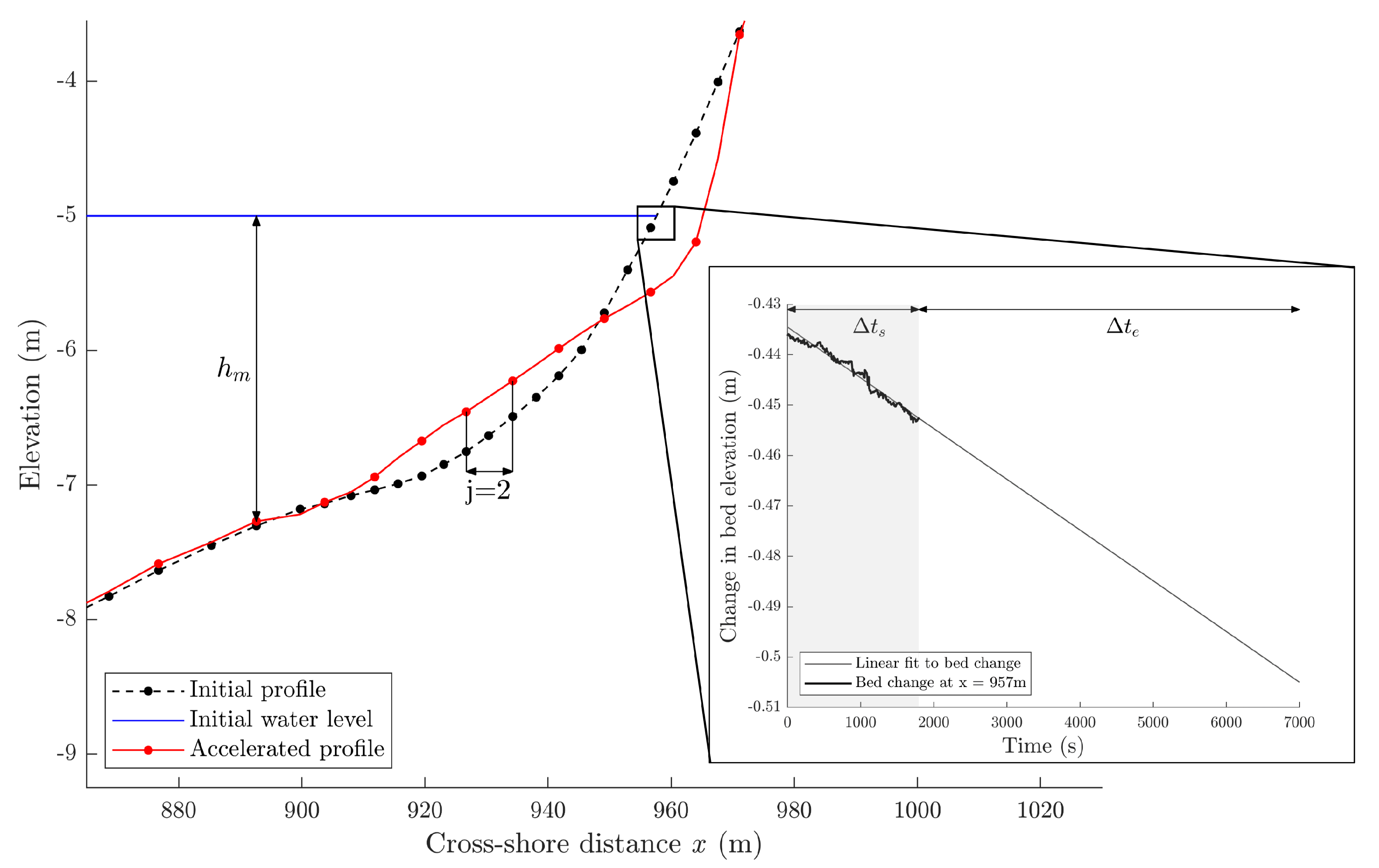
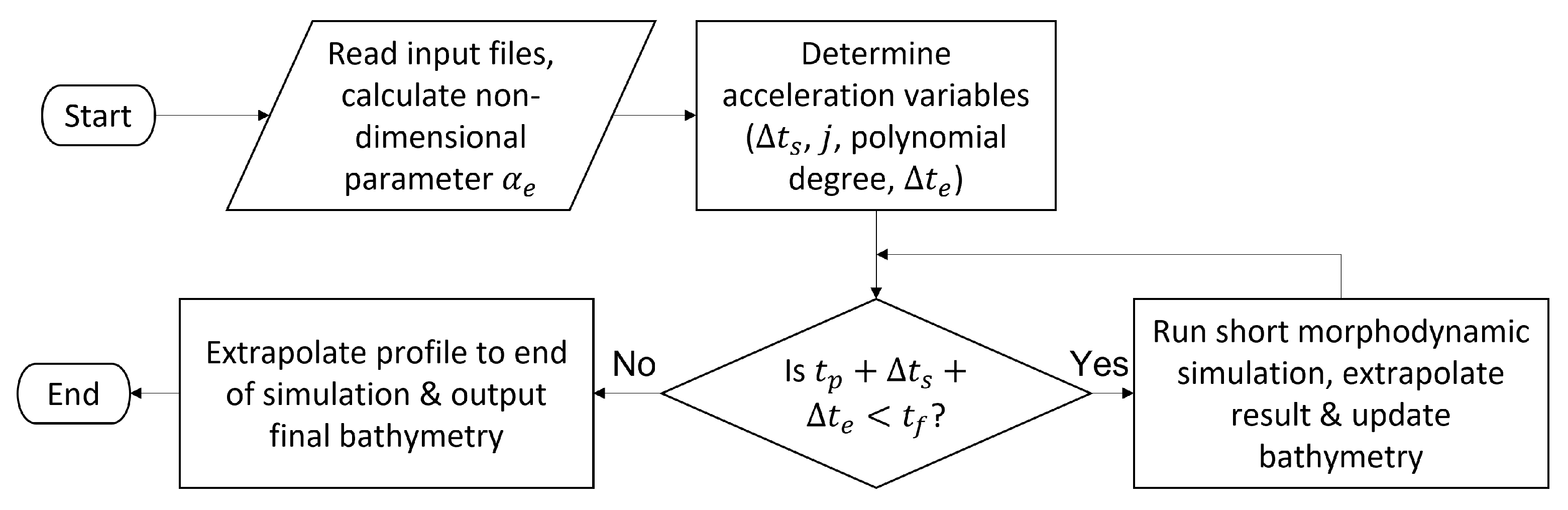
The proposed algorithm breaks up a full simulation of time length (where and are the final and initial times, respectively; typically ) into a series of cycles of fully coupled hydro-morphodynamic simulations, followed by extrapolation of the observed local trends. In each cycle, hydrodynamic and morphological processes are simulated in full (no acceleration) over a ‘simulation time’ interval . The results of this ‘mini-simulation’ are then processed, i.e., local evolution trends of the bed level are tracked for various points along x, where x is the cross-shore distance, then extrapolated for a time interval , i.e., the ‘extrapolation time’. The result is the predicted bed profile at time with respect to the beginning of the cycle, which is then fed into the hydro-morphodynamic solver; the cycle is repeated until the final time is reached or exceeded (see Figure 1). A detailed description of the extrapolation procedure and relevant criteria is provided next.
2.1.2. Detailed Description
Consider a time during the entire simulation (thus, ). Any hydro-morphodynamic numerical solver requires that the bed be discretised into n points (). At the beginning of the acceleration cycle, the bed is evolved using the same numerical time step for the hydrodynamic and bed-update equations, yielding the updated bed at . The next step is the selection of a subset of ; we set a sampling interval j (an integer) and then select every point in the whole set. Therefore, setting means using all of the original points , while , i.e., sampling every second point, reduces the number of original points by half. Our reason for introducing this variable is twofold: a value of can help to further accelerate the simulation, and it contributes to the removal of spurious oscillations that may otherwise potentially arise during the bed evolution. After setting a value of j, we are now working with the revised data , where , except if , in which case the last boundary point is appended to the array.
Figure 1 illustrates the sampling procedure for the particular case of . We then track the time evolution of every point , as illustrated in the inset of Figure 1, and all points are independently best-fitted with a curve using least-squares regression. For the curve fits, two options are assessed, namely, linear and quadratic polynomials (additional tests demonstrated that higher-order polynomials tended to decrease the quality of the final predictions). The fitted curves are evaluated at time ; in practice, can always be taken as zero within each acceleration cycle. For , the predicted (accelerated) bed is a smaller data array than the original bed vector; thus, to recover the original size, linear interpolation between points and is carried out, yielding a predicted bed at (the red curve in Figure 1). This beach profile is fed back into the hydro-morphodynamic solver and the cycle repeats until reaching the final simulation time . For stability purposes, the onshore and offshore boundaries of the profile should be selected such that their bed levels do not change during the whole simulation. It is expected that the proposed algorithm will reduce the number of numerical time steps in the hydro-morphodynamic solver by approximately a factor of .
The acceleration algorithm described above requires the setting of four different variables: (i) the time over which the hydro-morphodynamic solver evolves the full bed ; (ii) the sampling interval j, which leads to the (potentially reduced) bed profile vector ; (iii) the degree of the polynomial to be fitted to each point , which may be 1 (linear) or 2 (quadratic); and (iv) the extrapolation time . Ultimately, these variables depend on how erodible a given bed is for the hydrodynamic forcing under consideration; for example, we anticipate that a slow-evolving profile may require a larger value of in order to extract a meaningful evolution trend. Therefore, we introduce a non-dimensional variable related to the erodibility of a beach profile subject to wave forcing:
where is the median sediment grain diameter, is the median water depth (relative to the still water level, i.e., no tides are considered), and is the significant wave height. Thus, the (non-)erodibility parameter is defined such that larger values represent a reduced tendency towards erosion, e.g., coarse sediment and small waves propagating over a deep profile, and vice versa. In Section 2.3, we systematically arrive at the ‘optimal’ combination of the algorithm-defining variables (, , j and the degree of the fitted polynomial) as a function of . In Section 4, we discuss how may be modified in order to use this algorithm in other hydro-morphological conditions, such as the evolution of tidal inlets. Here, we employ XBeach as the hydro-morphodynamic solver and carry out the proposed algorithm externally via MATLAB. The structure of the algorithm implementation is shown in Figure 2.
2.2. Algorithm Calibration—Test Profiles
A series of beach profiles were used to calibrate the variables employed in the acceleration algorithm, which was then tested under a variety of conditions. Different beach slopes, wave energies, and sediment sizes were utilised, including idealised and real beach profiles.
2.2.1. Test Profile Shapes
Three types of test beach profile were modelled: linear, Dean, and measured (field) profiles. Linear and Dean profiles are described by mathematical functions, whereas measured profiles use data collected from real beaches in the UK. For the linear profiles, two slopes were modelled: a mild slope (1:100) and a steep slope (1:10). These values were based on profile slopes reported in [26], representing profiles across the southern and eastern coasts of the UK. Dean profiles are described by the function , where A is a constant (which depends, among other things, on the sediment size) and h is the local water depth [27]. For the sake of comparability, A was set by fitting a Dean profile to the measured profiles that we considered. Three sites along the South Coast of the UK were selected as measured test profiles: St. Ives, on the North Cornish coast; Christchurch Bay, on the Dorset coast; and Camber Sands, on the East Sussex coast. These selections were based on data from the Channel Coastal Observatory [28], and were extended offshore with a linear slope to avoid wave interaction with the offshore boundary.
2.2.2. Wave Forcing
The significant wave height () and peak wave period () for each measured profile site were taken from the Channel Coastal Observatory survey reports [28]. A JONSWAP (Joint North Sea Wave Analysis Project) spectrum was employed to describe the shape of the distribution used to generate the random wave time series at the offshore boundary, as this is the most commonly used wave spectrum in XBeach simulations [15]. The measured profile simulations used their respective wave characteristics, while the linear and Dean profile simulations used the most energetic of these (St. Ives) in order to induce the greatest morphological change.
The Linear Mild and Dean profiles were modelled with median sediment grain diameters representative of fine and coarse sand, i.e., 0.063 mm and 2.00 mm, respectively [29]. The Linear Steep profile was modelled with coarse sand only, as fine sand does not typically form a steep profile due to the asymmetry in the intensity of the wave–swash uprush and the returning backwash [30]. The median grain diameters used for the measured profiles were taken from the literature: 0.33 mm, 0.67 mm, and 1.00 mm for Camber Sands, St. Ives, and Christchurch Bay, respectively [26,31,32]. A full list of the profile characteristics and simulation parameters is provided in Table 1.
2.3. Algorithm Calibration—Tuning of Algorithm Variables
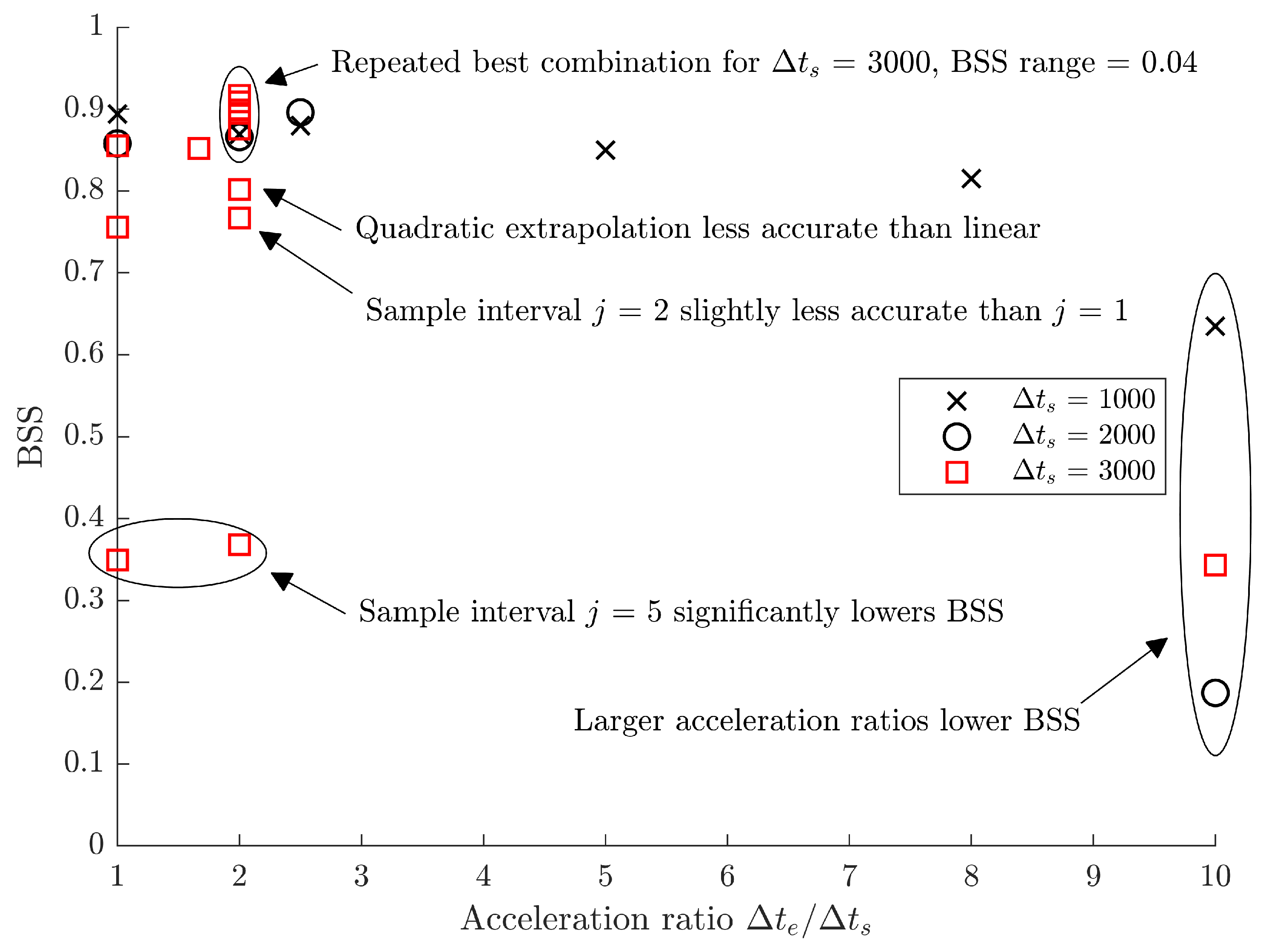
There are four tuning parameters in the algorithm, and we expect their optimal values to depend on . To calibrate the algorithm variables, we employed the following heuristic method. For a given beach profile and hydrodynamic forcing conditions, i.e., for a given value of , beginning with sensible arbitrary values of the algorithm variables ( s, ) and a linear extrapolation, we explored different ratios of acceleration to simulation times in the range . When the most promising value of was identified (for more on the performance evaluation, see below), we varied in the range of 1000 to 3000 s. As before, the most promising values of were identified, allowing us to assess the influence of changing the sample interval j in the range . The order of the extrapolation polynomial was investigated, although not exhaustively, as the preliminary tests showed that a linear extrapolation was almost always better than a quadratic one. A similar rationale was applied to all other profiles (values of ). To make the iteration process more efficient, results from profiles with similar values of were used to guide the iterations; for example, if it was clear for a given value of that a certain sample interval should be used, only this value was tested for other profiles with a similar value.
The performance of any given combination of the tuning parameters was evaluated by means of the Brier Skill Score (BSS), defined as follows:
where represents the predicted profile from the reference (non-accelerated) simulation, is the predicted profile from the accelerated simulation, and is the initial profile. To be more precise, , , and are vectors representing the discretised bed elevation profiles. Higher values of BSS (which has an upper limit of 1) represent better predictions. This metric has been used in similar sensitivity analyses (e.g., [17,33]). According to Ranasinghe et al. [33], a BSS value of 0.5 may be considered sufficiently accurate in complex engineering applications. Note that while the BSS has a theoretical upper limit of 1, this value would be difficult to achieve even for a non-accelerated profile due to the random nature of the boundary conditions (wave forcing), since repeating a simulation with the exact same parameters will yield slightly different results.
Figure 3 illustrates the calibration method employed for the Dean profile with coarse sediment (Dean Coarse). To enhance clarity, not all combinations of the tuning variables that we tested are included in this figure; the full information is available as part of the Supplementary Materials. Figure 3 evidences the heuristic nature of our calibration method, which by definition does not guarantee optimal results. However, clear patterns emerge, such as a decreasing performance of the algorithm for larger values of . All results are shown for a total simulation time of 24 h, which is consistent with a standard storm event and allows time for appreciable morphological change to occur while remaining within reasonable levels of computational cost. We additionally tested the BSS variation due to the probabilistic nature of the employed wave forcing conditions. After running a given scenario five times with no changes made to any parameters, the maximum (minimum) variation in BSS among all profiles was 0.18 (0.03), with an average variation of 0.08. For comparison, the same was done for XBeach’s built-in acceleration method (morfac), leading to maximum (minimum) variations in the BSS of 0.28 (0.05), with an average variation of 0.15.
Based on our extensive calibration method including more than 150 different combinations of the algorithm parameters (see Supplementary Materials), Table 2 provides a set of recommended values of the tuning parameters as a function of . While we acknowledge that these values are by no means optimal, we believe that they represent a good guide for practical applications of the proposed algorithm as well as a starting point for further refinements.
3. Results
In this section, the results of morphodynamic simulations accelerated via the proposed algorithm while using the recommended values of the -dependent variables shown in Table 2 are compared against simulations accelerated using XBeach morfac. The value of morfac for each scenario is set equal to the ratio of used in our acceleration algorithm; for example, as the Linear Steep test profile has an value greater than , we use s and . Therefore, we compare this profile against a morfac value of 2. The accuracy of both acceleration techniques is assessed relative to the full (non-accelerated) morphodynamic simulation, as detailed next.
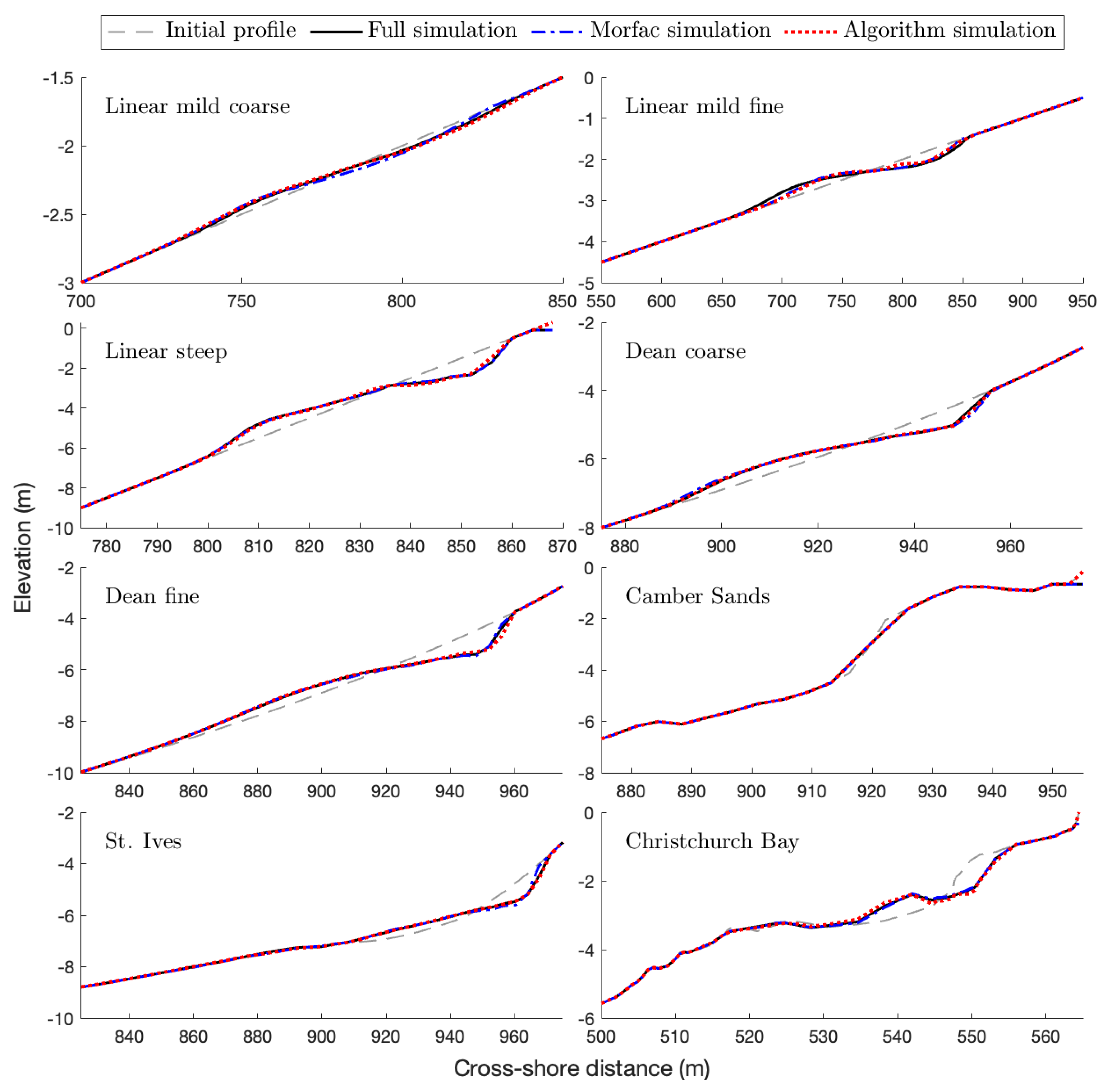
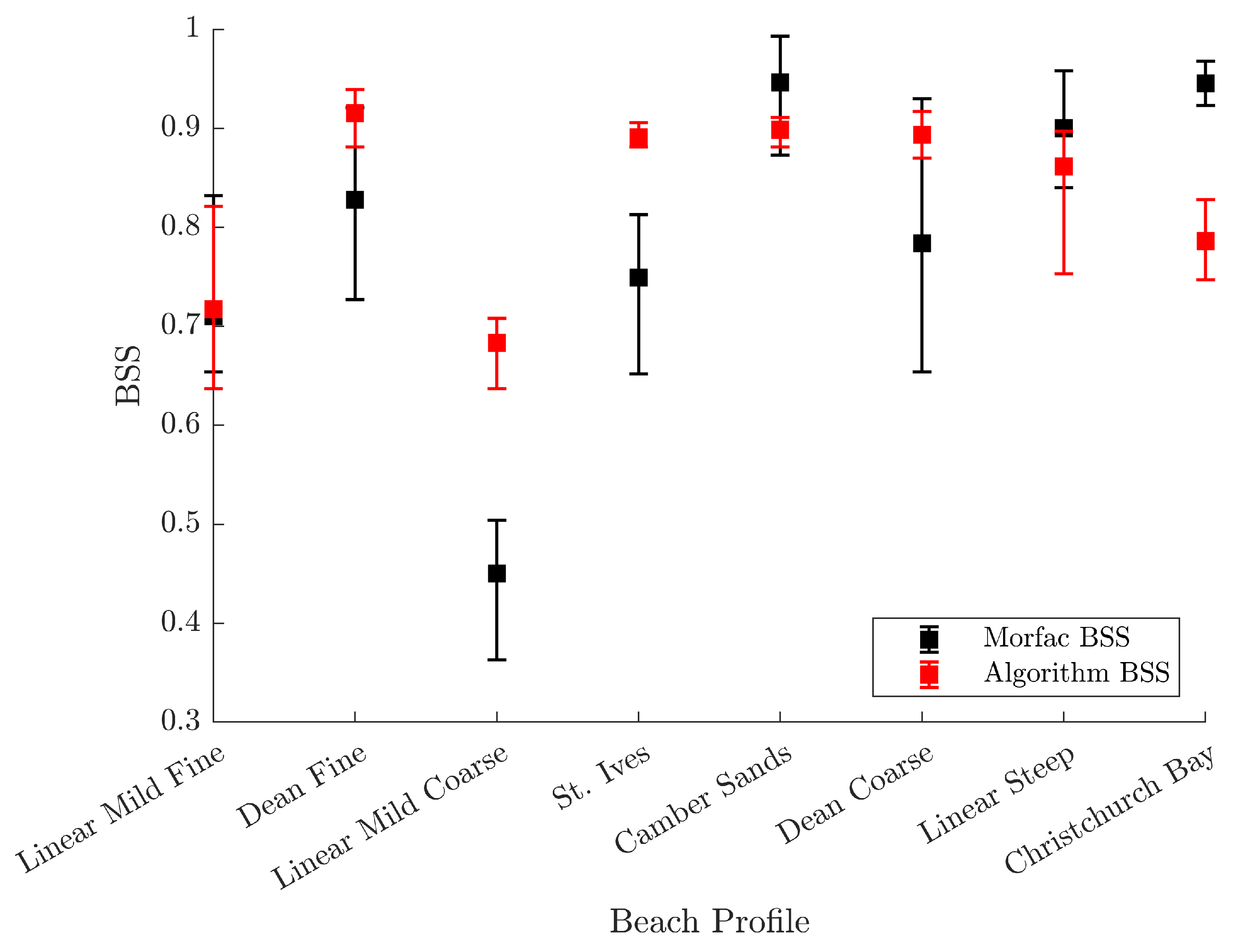
Figure 4, Figure 5, Figure 6 and Figure 7 illustrate the comparison between acceleration approaches from different perspectives. Figure 4 shows the predictions by both methods for all eight profiles considered. To enhance clarity, Figure 5 provides a qualitative comparison for the St. Ives and Linear Mild Coarse test profiles only, illustrating that while both approaches yield good predictions, the algorithm proposed here outperforms morfac in these two cases. A more quantitative comparison is shown in Figure 6, where only the difference between the accelerated profiles and the non-accelerated one for the Linear Mild and Dean profiles with coarse sediment is presented. A comprehensive comparison including all profiles is shown in Figure 7, which depicts the BSS for both methods and all profiles considered. From this figure it can be concluded that the proposed algorithm generally outperforms morfac. However, when considering the error bars representing the maximum and minimum BSS arising from five repetitions of each simulation, the performance of both methods can be said to be similar (for more details, see Section 4). While it is difficult to formulate an explanation of why morfac performs better for certain profiles, two potential reasons are worth exploring. First, this could be due to the heuristic calibration of the propsed algorithm, which is more refined for smaller values of , while morfac seems to perform better for larger values of . Second, morfac outperforms our algorithm in profiles where the onshore boundary shows a clear mismatch with the reference profile, such as Camber Sands and Christchurch Bay in Figure 4, which has an impact in terms of the BSS. This is a consequence of the requirement to fix this point. This problem has a simple practical solution: the onshore boundary can always be selected to be far enough to ensure that there is no influence of the waves on the morphology of this boundary. In fact, doing this is generally recommended in order to avoid numerical issues arising from the boundary conditions employed.
In addition to yielding accurate predictions, an acceleration approach must of course be evaluated based on its reduction of computational demands. We do this via two metrics. The first one is the total computational time, or computer elapsed time. This metric has an important caveat, in that morfac is built into the XBeach hydro-morphodynamic solver, while the proposed algorithm was programmed externally in MATLAB. Thus, the total computational cost includes the time required by XBeach to print the files, the time needed to communicate between XBeach and MATLAB, etc. This could make the total computational time favourably biased towards morfac. Thus, we introduce the total number of numerical time steps reported by XBeach, which is a more computer-independent proxy for the total computational cost of the simulation. Both metrics are normalised using the computational cost of the full simulation; for reference, we used a standard laptop with an Intel Core i5 processor and 8 GB of RAM. The results are shown in Figure 8. The proposed algorithm consistently outperforms morfac in terms of computational cost savings, with reductions in computational costs of up to 3.7 times larger than morfac (see Christchurch Bay). The reduction in numerical time steps provided by the algorithm is on average about 30% less than the approximate prediction presented in Section 2.1.2, i.e., a predicted reduction by a factor of approximately .
4. Discussion
On average, the algorithm-accelerated simulations were 9% more accurate, required 61% fewer time steps, and were 38% faster than the simulations accelerated using morfac. For the profiles where the algorithm was less accurate than morfac, the BSS of the algorithm was very high (greater than 0.8). Furthermore, the time saving of the algorithm shows less dependence on the profile (or more specifically, on the erodibility of the profile) than morfac. These metrics indicate that, for the profiles tested here, the algorithm proposed in this paper provides an improvement over a widely used method to accelerate morphodynamic simulations.
While it cannot be claimed that the proposed algorithm is always more accurate than the simple and popular technique morfac employed by XBeach, we believe that there are several arguments to put forward this algorithm as a promising alternative for accelerating morphodynamic simulations. First, while the accuracy of predictions as measured by the BSS is generally similar between both approaches, the algorithm consistently shows a larger reduction in computational time, a key feature that any acceleration method must present. This potential for computational time reduction is expected to become significantly more important for 2D problems. Second, the accuracy of the proposed algorithm shows less dependence on the profile under consideration (or rather the erodibility, as defined herein) compared to morfac, presenting larger promise for generalisation to arbitrary morphodynamic problems. Third, while the algorithm parameters have been carefully tuned as described in Section 2.3, this tuning is only heuristic; i.e., there is no guarantee that the recommended values are (anywhere near) optimal and the process is ultimately dependent of the set of profiles selected. In future work, this may be remedied by carrying out a more exhaustive exploration of the parameter space spanned by all relevant variables, perhaps making use of machine learning techniques. This could further improve the performance of the algorithm. Evidently, the conclusions obtained herein are the result of a limited (though diverse) set of beach profiles and forcing conditions; in the future, a more comprehensive comparison might include a larger set of beach profiles, event durations, and hydrodynamic conditions.
A disadvantage of our algorithm with respect to the simple morfac method is its relative complexity of implementation. However, to mitigate this potential weakness, we have made the codes freely available at https://github.com/sergio-maldonado/morpho_accelerate, and invite the community to use and further optimise them. The present paper has focused on the specific problem of beach profile evolution due to waves. This has been used as a way to introduce and illustrate the acceleration algorithm. However, the algorithm can be easily adapted to other morphodynamic problems by following the steps described here: first, define an erodibility parameter related to the problem at hand (e.g., for tidal inlets, in Equation (1) can be replaced by the tidal amplitude), then carry out a variable tuning procedure such as the one described in Section 2.3. Naturally, the actual values of the variables may vary widely depending on the morphodynamic problem under consideration; for example, for very slowly varying morphologies, much larger values of than those presented here may be achievable. Similarly, the algorithm may in principle be adapted to account for nature-based solutions, e.g., by accounting for the presence of vegetation in the definition of ; for example, in keeping with the present definition, variables whose increasing values tend to reduce erosion within the model employed, such as vegetation drag coefficient or canopy density, could be included in the numerator.
In the context of coastal adaptation to inherently uncertain future scenarios due to climate change and sea level rise, approaches that can rapidly explore long-term predictions of beach evolution (often of around 50 years; see, e.g., [34,35,36]) are crucial, especially because several scenarios must typically be considered [37]. The same is true for the modelling of larger spheres beyond the coast, e.g., the watershed–coast system, the integrated modelling of which is expected to become particularly important in the context of climate change [7]. This is because of the pressure that climate change can place on such systems, potentially leading to consequences extending beyond coastal morphology and into the fields of socio-economics or cultural heritage [38,39]. Noting that methods for speeding up morphodynamic simulations have remained virtually unchanged for decades, we propose a novel algorithm that represents a refreshing addition to the toolbox available to coastal scientists and engineers. The proposed algorithm represents a versatile tool that may in principle be generalised to arbitrary morphodynamic problems. It shows the potential to yield predictions with similar accuracy to those of the popular morfac method while consistently demonstrating superior capabilities in terms of computational time reduction.
5. Conclusions
There exists a very large gap between the timescales associated with hydrodynamic and morphological processes in the coastal environment. Because of this, coastal morphodynamic simulations tend to be computationally costly. This has motivated researchers to propose various methods of accelerating the morphological evolution process in order to reduce the computational cost of simulations. Most of these methods, which have not been revised for decades, rely on the presence of a clear periodic pattern in the hydrodynamics, e.g., tides, and apply a global measure to the bed, as is the case in XBeach’s morfac. In this paper, we propose a novel method for speeding up coastal morphodynamic simulations. Our proposed algorithm breaks up a simulation into a series of cycles, wherein a non-accelerated simulation stage is followed by an extrapolation stage. During the first non-accelerated simulation stage, the algorithm tracks local changes to the bed; then, during the second stage, it extrapolates the observed trends in time, feeding the extrapolated bed profile back to the hydro-morphodynamic solver. These cycles repeat until the final simulation time is reached. The algorithm requires the setting of four different parameters. Through an extensive calibration process, we obtained recommended (though not necessarily optimal) values of these parameters as a function of a non-dimensional variable defined in relation to the bed’s erodibility (; see Equation (1)). We tested the proposed algorithm on eight different beach profiles, including linear, Dean, and measured field profiles, and compared its performance against that of the popular morfac acceleration method built into XBeach. While both the proposed algorithm and morfac yield accelerated profiles with comparable accuracy, the former consistently shows a greater reduction in computational time as assessed by two different metrics. What is more, the proposed method can be further optimised by carrying out more comprehensive calibration of the algorithm parameters, and can in principle be adapted to various other coastal morphodynamic problems, including the use of nature-based solutions, via appropriate redefinition of . In light of the continued need for rapid simulations of coastal evolution for long-term predictions, particularly in the context of adaptation to uncertain climate change scenarios, we believe that the proposed method represents a promising addition to the toolbox employed by the community of coastal scientists, engineers, and policy makers.
Supplementary Materials
The following supporting information can be downloaded at: https://www.mdpi.com/article/10.3390/jmse11122314/s1.
Author Contributions
Conceptualization, E.N. and S.M.; methodology, E.N. and S.M.; software, E.N.; formal analysis, E.N. and S.M.; investigation, E.N.; resources, S.M.; writing E.N. and S.M.; visualization, E.N.; supervision, S.M. All authors have read and agreed to the published version of the manuscript.
Funding
This research received no external funding.
Institutional Review Board Statement
Not applicable.
Informed Consent Statement
Not applicable.
Data Availability Statement
The codes developed for this research are freely available at https://github.com/sergio-maldonado/morpho_accelerate. The data that support the findings of this study are available in the Supplementary Materials.
Acknowledgments
The authors wish to thank the three anonymous referees, whose insightful feedback led to significant improvement of this paper.
Conflicts of Interest
The authors declare no conflict of interest.
Abbreviations
The following abbreviations are used in this manuscript:
| JONSWAP | Joint North Sea Wave Analysis Project |
| BSS | Brier Skill Score |
References
- Roelvink, J.; Walstra, D.J.R.; van der Wegen, M.; Ranasinghe, R. Modeling of coastal morphological processes. In Springer Handbook of Ocean Engineering; Springer: Berlin/Heidelberg, Germany, 2016; pp. 611–634. [Google Scholar]
- Lesser, G.R.; Roelvink, J.V.; van Kester, J.T.M.; Stelling, G. Development and validation of a three-dimensional morphological model. Coast. Eng. 2004, 51, 883–915. [Google Scholar] [CrossRef]
- Dissanayake, P.; Brown, J.; Sibbertsen, P.; Winter, C. Using a two-step framework for the investigation of storm impacted beach/dune erosion. Coast. Eng. 2021, 168, 103939. [Google Scholar] [CrossRef]
- Simmons, J.A.; Harley, M.D.; Marshall, L.A.; Turner, I.L.; Splinter, K.D.; Cox, R.J. Calibrating and assessing uncertainty in coastal numerical models. Coast. Eng. 2017, 125, 28–41. [Google Scholar] [CrossRef]
- Karunarathna, H.; Brown, J.; Chatzirodou, A.; Dissanayake, P.; Wisse, P. Multi-timescale morphological modelling of a dune-fronted sandy beach. Coast. Eng. 2018, 136, 161–171. [Google Scholar] [CrossRef]
- Samaras, A.G.; Koutitas, C.G. The impact of watershed management on coastal morphology: A case study using an integrated approach and numerical modeling. Geomorphology 2014, 211, 52–63. [Google Scholar] [CrossRef]
- Samaras, A.G. Towards integrated modelling of Watershed-Coast System morphodynamics in a changing climate: A critical review and the path forward. Sci. Total Environ. 2023, 82, 163625. [Google Scholar] [CrossRef]
- Teeter, A.M.; Johnson, B.H.; Berger, C.; Stelling, G.; Scheffner, N.W.; Garcia, M.H.; Parchure, T. Hydrodynamic and sediment transport modeling with emphasis on shallow-water, vegetated areas (lakes, reservoirs, estuaries and lagoons). Hydrobiologia 2001, 444, 1–23. [Google Scholar] [CrossRef]
- Silver, J.M.; Arkema, K.K.; Griffin, R.M.; Lashley, B.; Lemay, M.; Maldonado, S.; Moultrie, S.H.; Ruckelshaus, M.; Schill, S.; Thomas, A.; et al. Advancing coastal risk reduction science and implementation by accounting for climate, ecosystems, and people. Front. Mar. Sci. 2019, 6, 556. [Google Scholar] [CrossRef]
- Dissanayake, D.; Roelvink, J.; Van der Wegen, M. Modelled channel patterns in a schematized tidal inlet. Coast. Eng. 2009, 56, 1069–1083. [Google Scholar] [CrossRef]
- Grunnet, N.M.; Walstra, D.J.R.; Ruessink, B. Process-based modelling of a shoreface nourishment. Coast. Eng. 2004, 51, 581–607. [Google Scholar] [CrossRef]
- Roelvink, J. Coastal morphodynamic evolution techniques. Coast. Eng. 2006, 53, 277–287. [Google Scholar] [CrossRef]
- Latteux, B. Techniques for long-term morphological simulation under tidal action. Mar. Geol. 1995, 126, 129–141. [Google Scholar] [CrossRef]
- Roelvink, D.; Reniers, A.; Van Dongeren, A.; De Vries, J.V.T.; McCall, R.; Lescinski, J. Modelling storm impacts on beaches, dunes and barrier islands. Coast. Eng. 2009, 56, 1133–1152. [Google Scholar] [CrossRef]
- Deltares. XBeach User Manual. 2020. Available online: https://xbeach.readthedocs.io/en/latest/user_manual.html (accessed on 13 August 2020).
- McCall, R.T.; De Vries, J.V.T.; Plant, N.; Van Dongeren, A.; Roelvink, J.; Thompson, D.; Reniers, A. Two-dimensional time dependent hurricane overwash and erosion modeling at Santa Rosa Island. Coast. Eng. 2010, 57, 668–683. [Google Scholar] [CrossRef]
- Vousdoukas, M.I.; Ferreira, Ó.; Almeida, L.P.; Pacheco, A. Toward reliable storm-hazard forecasts: XBeach calibration and its potential application in an operational early-warning system. Ocean Dyn. 2012, 62, 1001–1015. [Google Scholar] [CrossRef]
- Zimmermann, N.; Trouw, K.; De Maerschalck, B.; Toro, F.; Delgado, R.; Verwaest, T.; Mostaert, F. Scientific support regarding hydrodynamics and sand transport in the coastal zone: Evaluation of XBeach for long term cross-shore modelling. In WL Rapporten; WL-Publicaties: Antwerpen, Belgium, 2015. [Google Scholar]
- Van Rooijen, A.; McCall, R.; Van Thiel de Vries, J.; Van Dongeren, A.; Reniers, A.; Roelvink, J. Modeling the effect of wave-vegetation interaction on wave setup. J. Geophys. Res. Ocean. 2016, 121, 4341–4359. [Google Scholar] [CrossRef]
- Ruffini, G.; Briganti, R.; Alsina, J.M.; Brocchini, M.; Dodd, N.; McCall, R. Numerical modeling of flow and bed evolution of bichromatic wave groups on an intermediate beach using nonhydrostatic XBeach. J. Waterw. Port Coast. Ocean Eng. 2020, 146, 04019034. [Google Scholar] [CrossRef]
- Deltares. Delft3d-FLOW User Manual. 2023. Available online: https://content.oss.deltares.nl/delft3d4/Delft3D-FLOW_User_Manual.pdf (accessed on 25 November 2023).
- Roelvink, D.; Boutmy, A.; Stam, J.M. A simple method to predict long-term morphological changes. In Coastal Engineering 1998; American Society of Civil Engineers: Reston, VA, USA, 1999; pp. 3224–3237. [Google Scholar]
- Roelvink, J.; Jeuken, M.; Van Holland, G.; Aarninkhof, S.; Stam, J. Long-term, process-based modelling of complex areas. In Proceedings of the Coastal Dynamics’ 01, Lund, Sweden, 11–15 June 2001; pp. 383–392. [Google Scholar]
- O’Shea, M.; Murphy, J. Developing a Process Driven Morphological Model for Long Term Evolution of a Dynamic Coastal Embayment. Open J. Mar. Sci. 2020, 10, 93–109. [Google Scholar] [CrossRef]
- Carraro, F.; Vanzo, D.; Caleffi, V.; Valiani, A.; Siviglia, A. Mathematical study of linear morphodynamic acceleration and derivation of the MASSPEED approach. Adv. Water Resour. 2018, 117, 40–52. [Google Scholar] [CrossRef]
- Billson, O.; Russell, P.; Davidson, M. Storm waves at the shoreline: When and where are infragravity waves important? J. Mar. Sci. Eng. 2019, 7, 139. [Google Scholar] [CrossRef]
- Dean, R.G. Equilibrium beach profiles: Characteristics and applications. J. Coast. Res. 1991, 7, 53–84. [Google Scholar]
- Channel Coastal Observatory. Regional Coastal Monitoring Programmes. 2020. Available online: https://www.channelcoast.org/ (accessed on 7 January 2021).
- Cobb, F. Structural Engineer’s Pocket Book; CRC Press: Boca Raton, FL, USA, 2020. [Google Scholar]
- Komar, P. Beach Processes and Sedimentation; Prentice Hall: Hoboken, NJ, USA, 1998. [Google Scholar]
- Oyedotun, T. Sediment characterisation in an Estuary-beach system. J. Coast Zone Manag. 2016, 19, 2. [Google Scholar]
- Karunarathna, H.; Horrillo-Caraballo, J.M.; Ranasinghe, R.; Short, A.D.; Reeve, D.E. An analysis of the cross-shore beach morphodynamics of a sandy and a composite gravel beach. Mar. Geol. 2012, 299, 33–42. [Google Scholar] [CrossRef]
- Ranasinghe, R.; Swinkels, C.; Luijendijk, A.; Roelvink, D.; Bosboom, J.; Stive, M.; Walstra, D. Morphodynamic upscaling with the MORFAC approach: Dependencies and sensitivities. Coast. Eng. 2011, 58, 806–811. [Google Scholar] [CrossRef]
- Powell, E.J.; Tyrrell, M.C.; Milliken, A.; Tirpak, J.M.; Staudinger, M.D. A review of coastal management approaches to support the integration of ecological and human community planning for climate change. J. Coast. Conserv. 2019, 23, 1–18. [Google Scholar] [CrossRef]
- World Bank. Implementing Nature Based Flood Protection: Principles and Implementation Guidance; World Bank: Washington, DC, USA, 2017. [Google Scholar]
- Baustian, M.M.; Jung, H.; Bienn, H.C.; Barra, M.; Hemmerling, S.A.; Wang, Y.; White, E.; Meselhe, E. Engaging coastal community members about natural and nature-based solutions to assess their ecosystem function. Ecol. Eng. 2020, 143, 100015. [Google Scholar] [CrossRef]
- Schueler, K. Nature-Based Solutions to Enhance Coastal Resilience. 2017. Available online: https://publications.iadb.org/en/nature-based-solutions-enhance-coastal-resilience (accessed on 7 January 2021).
- Metcalf, S.J.; van Putten, E.I.; Frusher, S.; Marshall, N.A.; Tull, M.; Caputi, N.; Haward, M.; Hobday, A.J.; Holbrook, N.J.; Jennings, S.M.; et al. Measuring the vulnerability of marine social-ecological systems: A prerequisite for the identification of climate change adaptations. Ecol. Soc. 2015, 20, 35. [Google Scholar] [CrossRef]
- Reeder-Myers, L.A. Cultural heritage at risk in the twenty-first century: A vulnerability assessment of coastal archaeological sites in the United States. J. Isl. Coast. Archaeol. 2015, 10, 436–445. [Google Scholar] [CrossRef]
Figure 1.
Illustration of the proposed acceleration algorithm. The original profile (black dashed line) is evolved for ∼2000 s by simultaneously solving the hydrodynamic and bed update equations with the same numerical time step. The bed is then re-sampled (in this case, as , every other point is considered) and the local morphological changes are tracked. The inset shows the simulated evolution of the bed at m. The algorithm then extrapolates the observed trend (linearly, in this case) and predicts a bed change of approximately m at s. This is repeated for all other points in the profile, yielding the accelerated profile (the red curve), which is interpolated to recover the original resolution and then fed back into the hydro-morphodynamic solver. This cycle is repeated until reaching .

Figure 2.
Flowchart of the proposed acceleration algorithm.

Figure 3.
BSS performance metric vs. acceleration ratio for different values of the other algorithm parameters (, sampling interval j, and degree of polynomial fit); see annotations. For illustration purposes, only the Dean profile with coarse sediment () is shown here.
Figure 3.
BSS performance metric vs. acceleration ratio for different values of the other algorithm parameters (, sampling interval j, and degree of polynomial fit); see annotations. For illustration purposes, only the Dean profile with coarse sediment () is shown here.

Figure 4.
Comparison of profile predictions by the present algorithm and morfac for all beach profiles considered.
Figure 4.
Comparison of profile predictions by the present algorithm and morfac for all beach profiles considered.

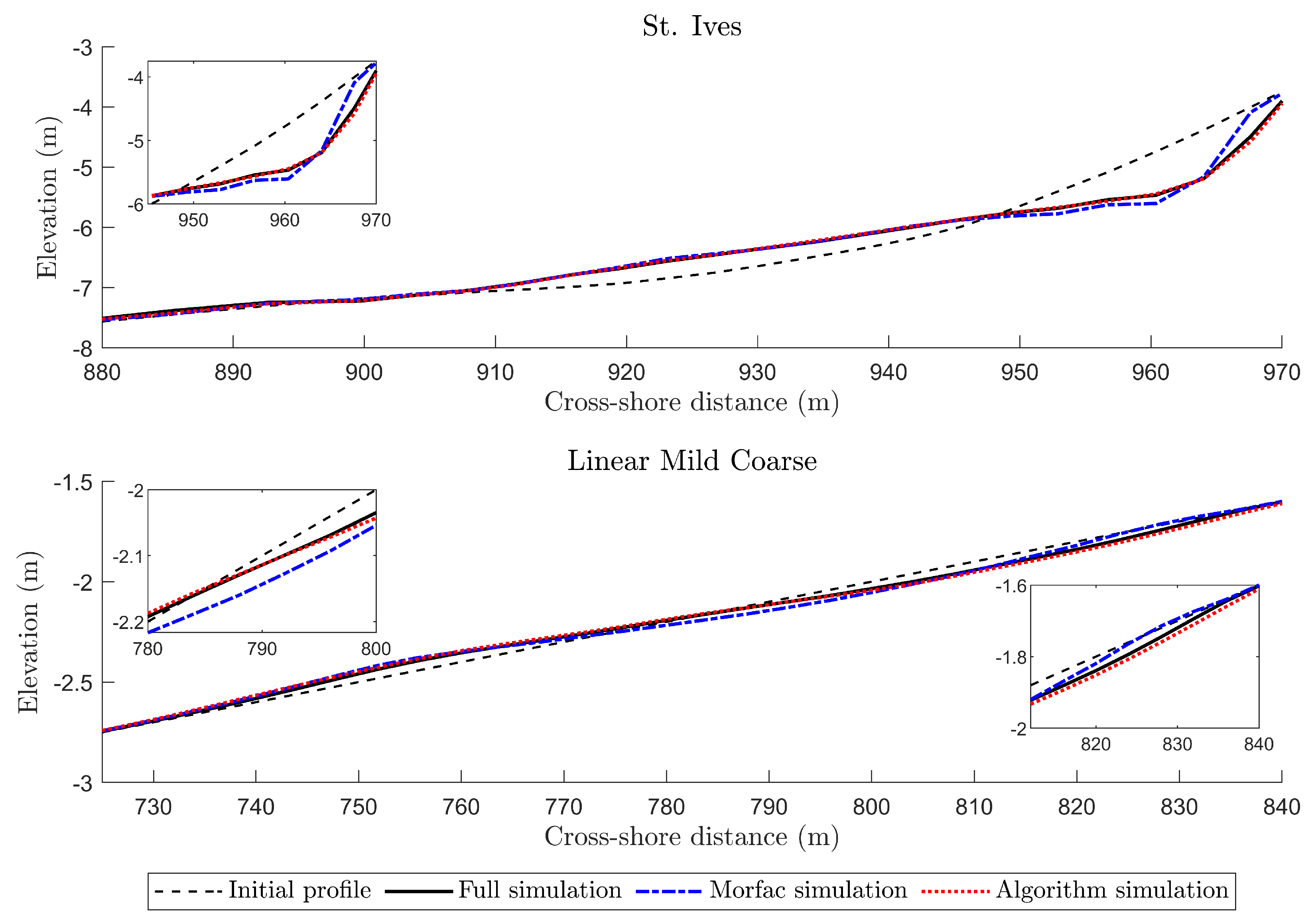
Figure 5.
Comparison of profile predictions for St. Ives and Linear Mild Coarse profiles, showing that the proposed algorithm-accelerated simulation agrees better with the full simulation prediction than the morfac-accelerated simulation.
Figure 5.
Comparison of profile predictions for St. Ives and Linear Mild Coarse profiles, showing that the proposed algorithm-accelerated simulation agrees better with the full simulation prediction than the morfac-accelerated simulation.

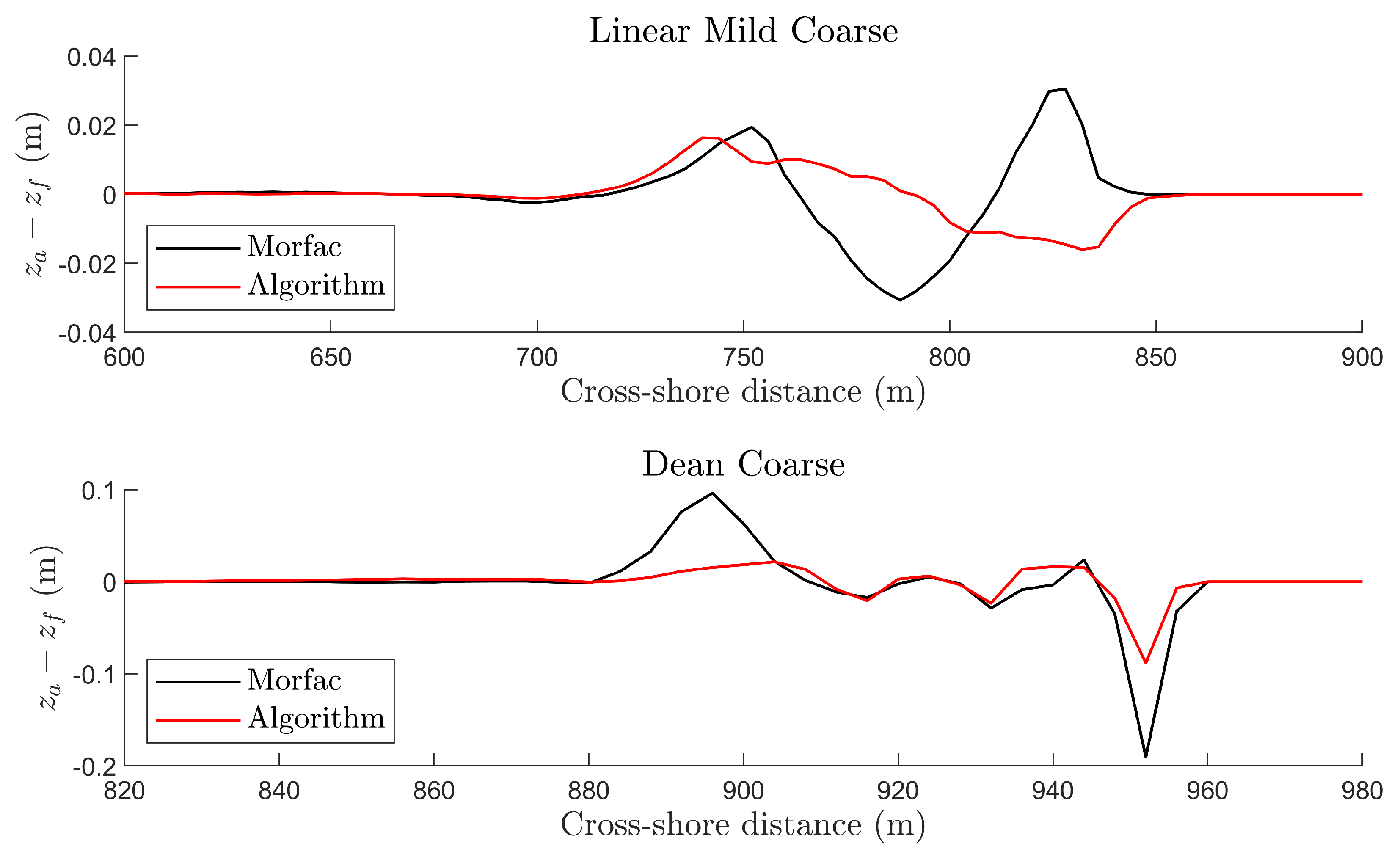
Figure 6.
Difference between the accelerated simulations using both morfac and the proposed algorithm and the non-accelerated simulation (results shown for the Linear Mild Coarse and Dean Coarse profiles only).
Figure 6.
Difference between the accelerated simulations using both morfac and the proposed algorithm and the non-accelerated simulation (results shown for the Linear Mild Coarse and Dean Coarse profiles only).

Figure 7.
BSS accuracy metric for morfac and the proposed algorithm for all test profiles. The error bars represent the maximum and minimum from five repetitions of each simulation, while the squares represent the average values. The erodibility of the profiles decreases from left to right, i.e., increases from left to right.

Figure 8.
Computational cost for morfac and the proposed algorithm normalised by that of the full simulation, employing two different metrics: computer elapsed time and number of numerical time steps reported by XBeach. Error bars are not shown, as the variation between repetitions of each simulation was minimal.


Table 1.
Morphological and hydrodynamic parameters of the test profiles.
| Test Profile | (m) | (s) | (mm) | (m) | |
|---|---|---|---|---|---|
| Linear Mild Fine | 1.58 | 10.55 | 0.063 | 3.00 | |
| Linear Mild Coarse | 1.58 | 10.55 | 2.000 | 3.00 | |
| Linear Steep | 1.58 | 10.55 | 2.000 | 41.10 | |
| Dean Fine | 1.58 | 10.55 | 0.063 | 15.16 | |
| Dean Coarse | 1.58 | 10.55 | 2.000 | 15.16 | |
| St. Ives | 1.58 | 10.55 | 0.670 | 9.44 | |
| Christchurch Bay | 0.64 | 9.03 | 1.000 | 16.98 | |
| Camber Sands | 0.75 | 5.63 | 0.330 | 12.04 |
Table 2.
Summary of recommended values for the algorithm parameters as a function of .
| Range | (s) | (s) | j | Polynomial Fit |
|---|---|---|---|---|
| 3000 | 5000 | 5 | Linear | |
| 3000 | 5000 | 1 | Linear | |
| 2000 | 5000 | 1 | Linear | |
| 3000 | 6000 | 1 | Linear |
Disclaimer/Publisher’s Note: The statements, opinions and data contained in all publications are solely those of the individual author(s) and contributor(s) and not of MDPI and/or the editor(s). MDPI and/or the editor(s) disclaim responsibility for any injury to people or property resulting from any ideas, methods, instructions or products referred to in the content. |
© 2023 by the authors. Licensee MDPI, Basel, Switzerland. This article is an open access article distributed under the terms and conditions of the Creative Commons Attribution (CC BY) license (https://creativecommons.org/licenses/by/4.0/).
Share and Cite
MDPI and ACS Style
Newell, E.; Maldonado, S. Acceleration of Morphodynamic Simulations Based on Local Trends in the Bed Evolution. J. Mar. Sci. Eng. 2023, 11, 2314. https://doi.org/10.3390/jmse11122314
AMA Style
Newell E, Maldonado S. Acceleration of Morphodynamic Simulations Based on Local Trends in the Bed Evolution. Journal of Marine Science and Engineering. 2023; 11(12):2314. https://doi.org/10.3390/jmse11122314
Chicago/Turabian StyleNewell, Ellie, and Sergio Maldonado. 2023. "Acceleration of Morphodynamic Simulations Based on Local Trends in the Bed Evolution" Journal of Marine Science and Engineering 11, no. 12: 2314. https://doi.org/10.3390/jmse11122314
Note that from the first issue of 2016, this journal uses article numbers instead of page numbers. See further details here.