Article

Sea Ice as a Factor of Primary Production in the European Arctic: Phytoplankton Size Classes and Carbon Fluxes

1
Shirshov Institute of Oceanology, Russian Academy of Sciences, 36 Nakhimovsky Prospect, 117997 Moscow, Russia
2
Winogradsky Institute of Microbiology, Research Center of Biotechnology, Russian Academy of Sciences, Leninsky Prospect, 33, Build. 2, 119071 Moscow, Russia
3
Moscow Institute of Physics and Technology, 9 Institutskiy per., 141701 Dolgoprudny, Russia
*
Author to whom correspondence should be addressed.
J. Mar. Sci. Eng. 2023, 11(11), 2131; https://doi.org/10.3390/jmse11112131
Submission received: 29 May 2023 / Revised: 27 October 2023 / Accepted: 31 October 2023 / Published: 8 November 2023
(This article belongs to the Special Issue Phytoplankton Dynamics and Biogeochemistry of Marine Ecosystems)

Abstract

:
The seasonally ice-covered marine region of the European Arctic has experienced warming and sea ice loss in the last two decades. During expeditions in August 2020 and 2021, new data on size-fractioned primary production (PP), chlorophyll a concentration, phytoplankton biomass and composition and carbon fixation rates in the dark were obtained in the marginal ice zone (MIZ) of the Barents Sea, Nansen Basin and Greenland Sea to better understand the response of Arctic ecosystems to ongoing climate changes. Four different situations were observed in the study region: (i) a bloom of the large-cell diatom Podosira glacialis, whose biomass was trapped in a strong halocline at the edge of a dense ice cover; (ii) a bloom of the chain-like colonies of Thalassiosira diatoms on the shelf in mixed waters in fields of shallow ice that could be supported by “fresh” elements in the polynya condition, as well as by terrestrial run-off and drifting ices; at the late stage, this bloom was accompanied by intensive growth of Phaeocystis pouchetti; (iii) dominance of small-cell phytoplankton under weakened stratification and the significant influence of the Atlantic water, depleted of microelements and silicates; (iv) dominance of dinoflagellates of eutrophic water in the contact zone between the water masses of Arctic origin and Atlantic origin in clear water under conditions of increased light intensity. The >10 µm phytoplankton cell size group increased its relative contribution to PP as a response to stratification, light and nutrient load associated with sea ice conditions. Small phytoplankton with sizes < 2 µm formed the basis of total PP in the MIZ regardless of the state of the sea ice.

1. Introduction

In the Arctic Ocean (AO), the area and thickness of the ice cover have been decreasing during the last two decades [1,2]. Positive trends for the primary production (PP), registered from satellite-based estimates [3,4,5,6], have been found for almost all seas of the AO. A significant effect from the expansion of ice-free areas is observed in the seas exposed to the strong influence of river runoff—the Kara, Laptev and East Siberian Seas (56%)—and to a lesser extent in the seas influenced by the North Atlantic—the Barents Sea (24%) and the Greenland Sea (10%).
The triggering factor for phytoplankton blooms in the Arctic Basin is the spring increase in solar activity. Exceeding the threshold values of photosynthetically active radiation (PAR) under optically transparent annual ice causes a local increase in phytoplankton biomass (PB), which is observed up to ~84–86° N (Amundsen and Nansen basins) [7,8]. Here, the phytoplankton growth rate increases from February (at ~71° N, Baffin Sea) and reaches its maximum in April–May under conditions of the solid ice cover, i.e., two months before its melting and destruction [9].
Spring phytoplankton blooms are observed during the seasonal ice breakup in the European Arctic. Blooms develop in the marginal ice zone (MIZ) as a result of meltwater entering the surface mixed layer (SML) and increasing water column stability, leading to PB accumulation [5,10]. Phytoplankton bloom in summer and continue into the spring bloom, which begins under ice cover in lenses of brackish water [11].
The high spatial heterogeneity of the hydrophysical characteristics of the MIZ leads to redistribution of the light regime due to drifting ice fields, biomass and nutrients under the influence of sporadic phenomena (mixing, eddies, etc.) [12]. Thus, the temporal development of blooms does not follow a smooth curve (growth, peak, decline, post-bloom) within the MIZ but is characterized by spatial patchiness in eddy structures [13]. Nevertheless, all stages of the seasonal succession of phytoplankton can be simultaneously observed in this zone [14].
Phytoplankton blooms with different compositions of dominant species that leave different biogeochemical “footprints” in the water column and affect element fluxes and ecosystem functioning. An approach based on estimating the contribution of phytoplankton of different sizes to biomass and PP allows the characterization of the food web, the carbon fixation rate and the amount of matter exported to the deep ocean [15]. In particular, the predominance of picophytoplankton (<2 μm) and nanophytoplankton (2–20 μm) indicates the regeneration of organic matter through the microbial food web and its accumulation in the euphotic zone (Zeu) due to the low sedimentation of small cells. In contrast, the dominance of microphytoplankton (>20 μm) implies the high sedimentation rate of recently assimilated carbon to the bottom. According to Falkowsky et al. [16], when light conditions improve at the end of winter in seas with pronounced seasonal phenomena or due to nutrient pulsation in the Zeu, the ecosystem is perturbed, which causes an outbreak of large phytoplankton development. After resource depletion, the ecosystem returns to an equilibrium state where regenerated PP prevails and that is dominated by small phytoplankton.
In the European Arctic, diatom and haptophyte populations develop during the spring bloom in response to system-wide environmental shifts and the increasing influence of intermediate water of Atlantic origin (AW) on the productive layer observed since the 1990s [7,11,17]. Among haptophytes, Phaeocystis pouchetti dominates, inhabiting single cells of ~5 µm size and colonies of cells of up to 2 mm. The successful development of this species may be related to its adaptation to the rapid change in the light regime under the conditions of drifting ice fields, low concentrations of nutrients and weak stratification [7,11]. Regional diatoms belong to the microphytoplankton and, in contrast, are sensitive to the reduction in both the ice cover area and ice thickness. It has been shown [18] that silicates may decrease due to the increasing influence of AW. Picophytoplankton consists of endemic Arctic picoeukaryotes and picocyanobacteria associated with both AW and Polar-origin water (PW) [19,20,21].
There are limited estimates for PP and the contribution of different size groups of phytoplankton in the MIZ at high latitudes. However, these studies are rather significant under the conditions of the “atlantification” of the Eurasian Basin for understanding the carbon cycle changes in the recent ocean. Therefore, our work aimed to study the contribution of different size groups of phytoplankton to PP and chlorophyll a (Chl a) concentration in the MIZ of the European Arctic seas.
The following questions are addressed in this study:
(i)
How does the contribution of phytoplankton of different sizes to PP change at high and low sea ice concentrations in the European Arctic in summer?
(ii)
What environmental factors influence the species and size structure of phytoplankton in the European Arctic in summer?

2. Materials and Methods

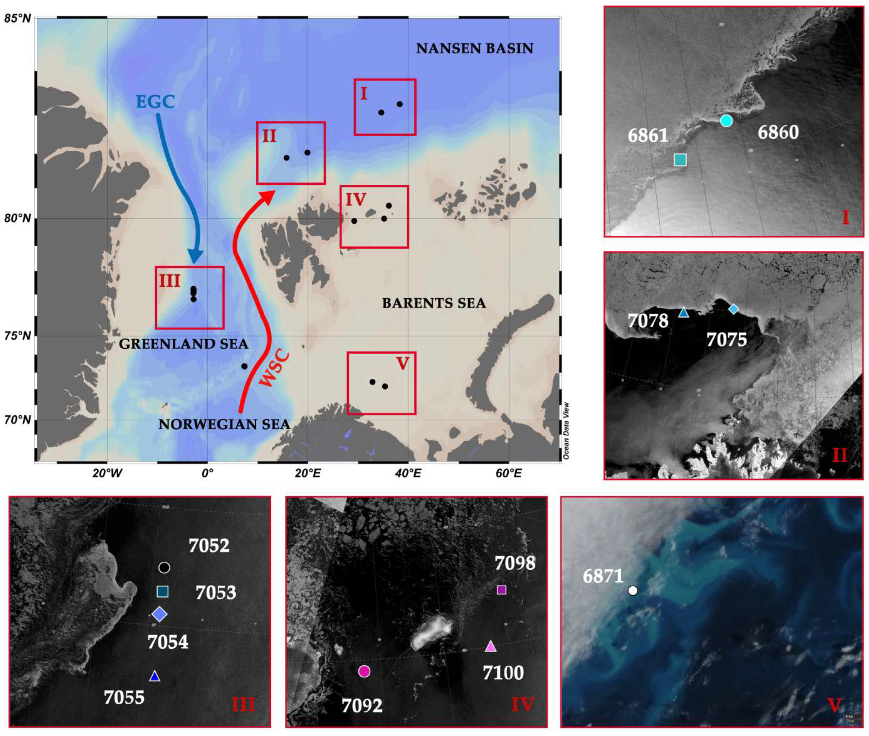
2.1. Study Area and Fieldwork Description

The studied region is located in the area of interaction between two major water masses, namely AW and PW. The data were obtained in the European Arctic during two research cruises of the RV Akademik Mstislav Keldysh (the 80th in August 2020 and the 84th in July–August 2021) [22,23]. The cruises covered the Norwegian, Greenland and Barents Seas and Nansen Basin (Figure 1). Here, we report the results of the size-fractionated structure of Chl a, phytoplankton and PP collected at ten stations located in the MIZ of the study region. In the Nansen Basin, the stations (sts.) 6860 and 6861 were sampled on August, 17th and 18th, 2020, respectively; sts. 7075 and 7078 on August, 11 and 12, 2021. The results for the Greenland Sea (sts. 7052–7055) and the northern Barents Sea (sts. 7092, 7098, 7100) were obtained in 2021 on August, 2nd and 3rd in the first area and on August, 18th and 19th in the second one. In addition, four sampling stations were located in contrasting areas of the southern Barents Sea (st. 6871 in 2020 and st. 7106 in 2021; both stations were sampled on 22 August) and Norwegian Sea (st. 6838 on 8 August 2020 and st. 7048 on 30 July 2021), free of seasonal ice cover, where the samples were also divided into fractions.

2.2. Sampling, Hydrography, Light Conditions and Chemical Analyses

At all stations, CTD (conductivity–temperature–depth) casts were conducted. A SBE9 + CTD underwater system (Sea-Bird Electronics Inc., Bellevue, WA, USA) was used, interfaced with a sampling carousel of 24 Niskin bottles (10 L volume of each bottle). For biological and chemical analysis, seawater samples were usually collected to at least 300 m. Each sampling depth was determined in order to cover the SML, depth of maximum change in the density of the water column, pycnocline, depth where the pycnocline ends, fluorescence maximum and depth of Zeu. The SML was defined based on the value of 0.03 kg∙m−3 deference in water density at the depth from the surface density (Δσ).
Incident PAR was continuously recorded using a LI–190SA planar sensor (LI-COR Environmental, Lincoln, NE, USA) mounted on the foredeck high above a vessel’s deck. The two LI-192SA sensors were used to measure the underwater irradiance before hydrocasts. Each sensor measures the PAR from all angles in one hemisphere. The results of the measurements were cosine corrected and expressed as photosynthetic photon flux density.
The PAR level for each sampling depth in the MIZ was calculated with the model:
PAR(z) = PAR(0)exp(−Kdz),
where PAR(0) is the PAR just below the surface and Kd is the averaged vertical attenuation coefficient of planar downwelling irradiance for the layer of 1% PAR depth. In the MIZ, the ponded ice albedo (0.2) was used to obtain estimates of the surface layer scattering.
As a rule, the samples for hydrochemical analyses were collected at the same depths as those chosen for measuring the biological parameters. Analyses of dissolved mineral phosphorous (PO4), silicate (Si(OH)4), nitrate (NO3) and nitrite (NO2) nitrogen were carried out according to standard methods [24] on board the vessel using a UV-VIS spectrophotometer HACH DR6000 (HACH-LANGE GmbH, Düsseldorf, Germany). The nitrate and nitrite concentrations were summarized and presented as NO3. Total phosphorous weas analysed as dissolved mineral phosphorous following mineralization (detected in 2021 only). The detection limits for NO3, NO2 and PO4 were <0.02 μM and for NH4 and Si(OH)4 were ~0.05 μM.

2.3. Standing Stock of Phytoplankton

A 500 mL sample for the phytoplankton study was collected from each depth and fixed with 40% neutralized formaldehyde to a final concentration of 1%. The phytoplankton cells were concentrated by the twofold method. Initially, they were concentrated in vials by settling for at least two weeks and decanted to a volume of 10 mL. Then, the precipitate was poured into a test tube and, after settling for several days and decanting, the volume was adjusted to 2–3 mL. The abundance of phytoplankton was determined by using an Ergoval light microscope (Karl Zeiss, Jena, Germany) with 16 × 10 to 16 × 40 magnifications. Cells with linear dimensions < 20 μm were counted using a Naujotte chamber (0.05 mL); the large cells were counted using a Naumann chamber (1 mL). The cells were counted in 2–3 replicates depending on the concentration of cells. Unidentified species of the size group 4–10 μm were assigned to the small flagellate group. Phytoplankton ≤ 2 µm is size was assigned to the picoplankton group.
Cell volumes were calculated from cell geometry after measuring the size [25,26]. To obtain estimates of the carbon biomass, we applied the allometric equations of Menden-Deuer and Lessard [27]. Species identification was based on morphology and was conducted following references [28,29] and the World Register of Marine Species (accessed on 1 March 2023 http://www.marinespecies.org). The trophic status of the identified species was determined using the Northern European Microalgae database (accessed on 4 March 2023 http://nordicmicroalgae.org/) and other web sites (or links to individual species).
Samples for Chl a determination were collected from 8–12 depths ranging from 0 to 150 m. A 300 mL water sample was serially filtered through a 10 μm polycarbonate filter by gravity filtration, a 2 µm polycarbonate filter (Millipore, Burlington, MA, USA) and a GF/F filter of 0.7 μm nominal pore size (Whatman, GB, Maidstone, UK). A filtration vacuum of ≤200 mbar was used for 0.2 and 2 μm filters. The Chl a concentration was determined fluorometrically in 90% acetone overnight extracts using a Trilogy Laboratory Fluorometer model # 7200-000 (Turner Designs, San Jose, CA, USA), as described by Holm-Hansen [30].

2.4. Primary Production

PP was measured via the 14C uptake technique [31]. For each sampling depth, we collected seawater and poured it into 3 borosilicate glass bottles of 310 mL in volume (2 light and 1 dark). A total of 5–10 µCi of labeled bicarbonate solution (Amersham, GB) was added to these. The samples were incubated in an on-deck-type incubator in the neutral density aluminum screens that simulated the attenuation of PAR in the range from 90 to 1% of the surface flux. We tested the irradiation scattering of the screens using BIC-2104Z1041 (Biospherical Instruments, San Diego, CA, USA) at four wavelengths (443, 490, 555 and 625 nm). The maximum irradiance transmission was a blue-green light spectrum (peak at 490 nm) that is close to the depth-related changes in the light spectrum for clear ocean [32]. The water was continuously pumped through the incubator to maintain the temperature at an in situ value with an aquarium chiller TECO TK 1000 (TECO s.r.l., Ravenna, Italy). The period of incubation was 24 h. At stations 6860 and 7054, the samples were incubated for 8–l0 h in the sea, suspended at depths corresponding to their depth of sampling. In situ incubations allow for exposing the samples to the natural temperatures and light levels [33,34,35]. After incubation, the samples were filtered sequentially through 10 µm and 2 µm polycarbonate filters (Millipore, Burlington, MA, USA) and 0.2 µm nylon filters (Technofilter RME, Vladimir, Russia) under a low-pressure vacuum ≤ 200 mbar. All filters were cleansed with 1% v/v hydrochloric acid to remove non-fixed inorganic 14C and then transferred to glass scintillation vials to which 10 mL of scintillation cocktail (EcoLume, MP Biomedicals, Santa Ana, CA, USA, or Ultima Gold XR, PerkinElmer, Inc., Waltham, MA, USA) was added. The incorporated 14C was determined with a scintillation counter (TRI-Carb TR, Packard, Detroit, MI, USA). The samples were counted 2 to 3 times until the counts were close in number. DPM values were converted to daily productivity rates, assuming 5% isotope discrimination. For 2 stations where in situ incubations were performed, PP was corrected by the daily PAR data.
Based on the PP measurements, the following further calculations were made:
(i)
PChl—the particulate PP rate normalized to Chl a at individual depths that follow a saturating function of daily light availability;
(ii)
PC—the particulate PP rate normalized to the phytoplankton carbon biomass and equivalent to a biomass grow rate = turnover rate [36,37].

2.5. Analysis of the Relationship between Phytoplankton and Environmental Factors

To assess the relationship between phytoplankton abundance indicators and various environmental factors, single linear regression analysis was used, and the least squares method was used to obtain model parameters. The p-value was established as less than 0.05. The Fisher–Snedecor test was applied to determine the model’s significance.

3. Results

3.1. Sea Ice Cover in August 2020 and 2021

Based on averaged data retrieved from the Sentinel-1A/B spaceborne synthetic aperture radars for August 2020 and 2021, the sea ice conditions in the MIZ of the study region differed significantly. In 2020 at stations 6860 and 6861 located in the Nansen Basin (~82° N), a northward shift of the compact ice cover edge was observed (Figure 1 (area I)). The edge of the compact ice cover retained its quasi-stationary position at stations 7075 and 7078, whereas in general, the basin was free of dense ice cover (Figure 1 (area II)). The transport of broken ice in a southwestern direction was observed in the northern part of the Barents Sea (Figure 1 (area IV)), where the stations were located in the Kvitøya Trough (st. 7092) and east of Kvitøya Island at the branch of the inflow from the Franz Victoria Trough (sts. 7097 and 7100). In the Greenland Sea (Figure 1 (area III)), sts. 7052–7055 were located ~10 km from floating ice in highly dynamic turbulent waters at the periphery of the East Greenland Current.

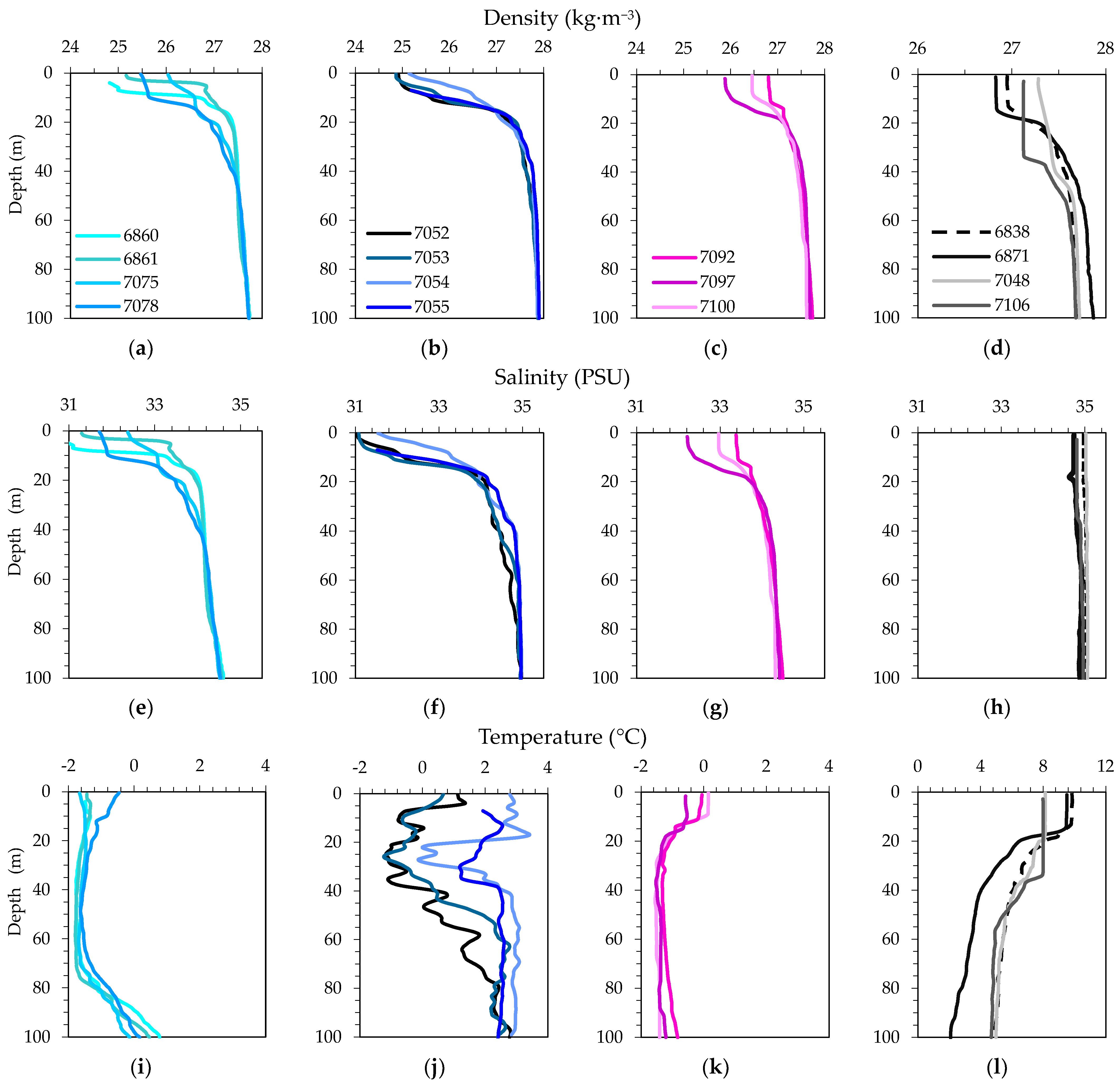
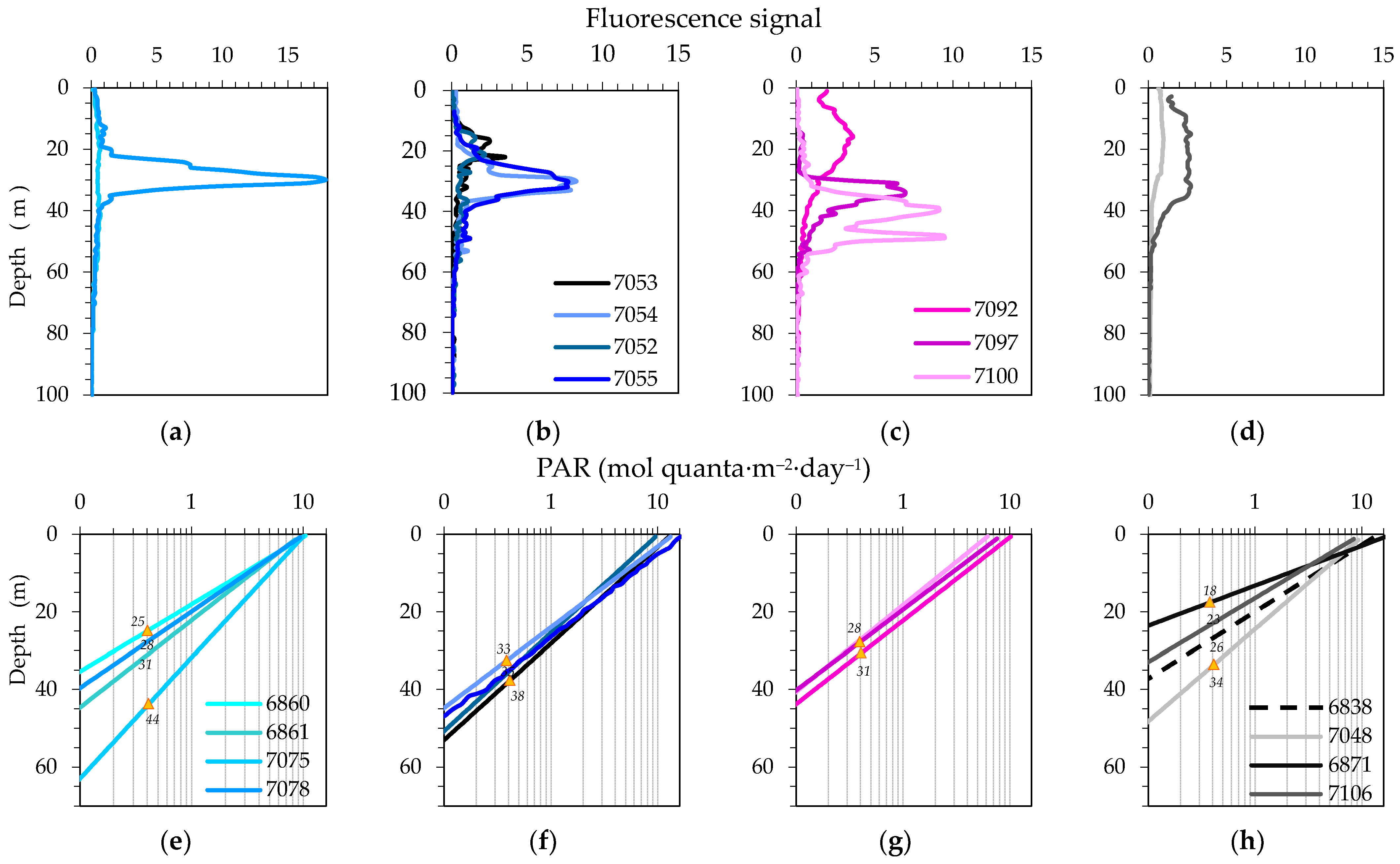
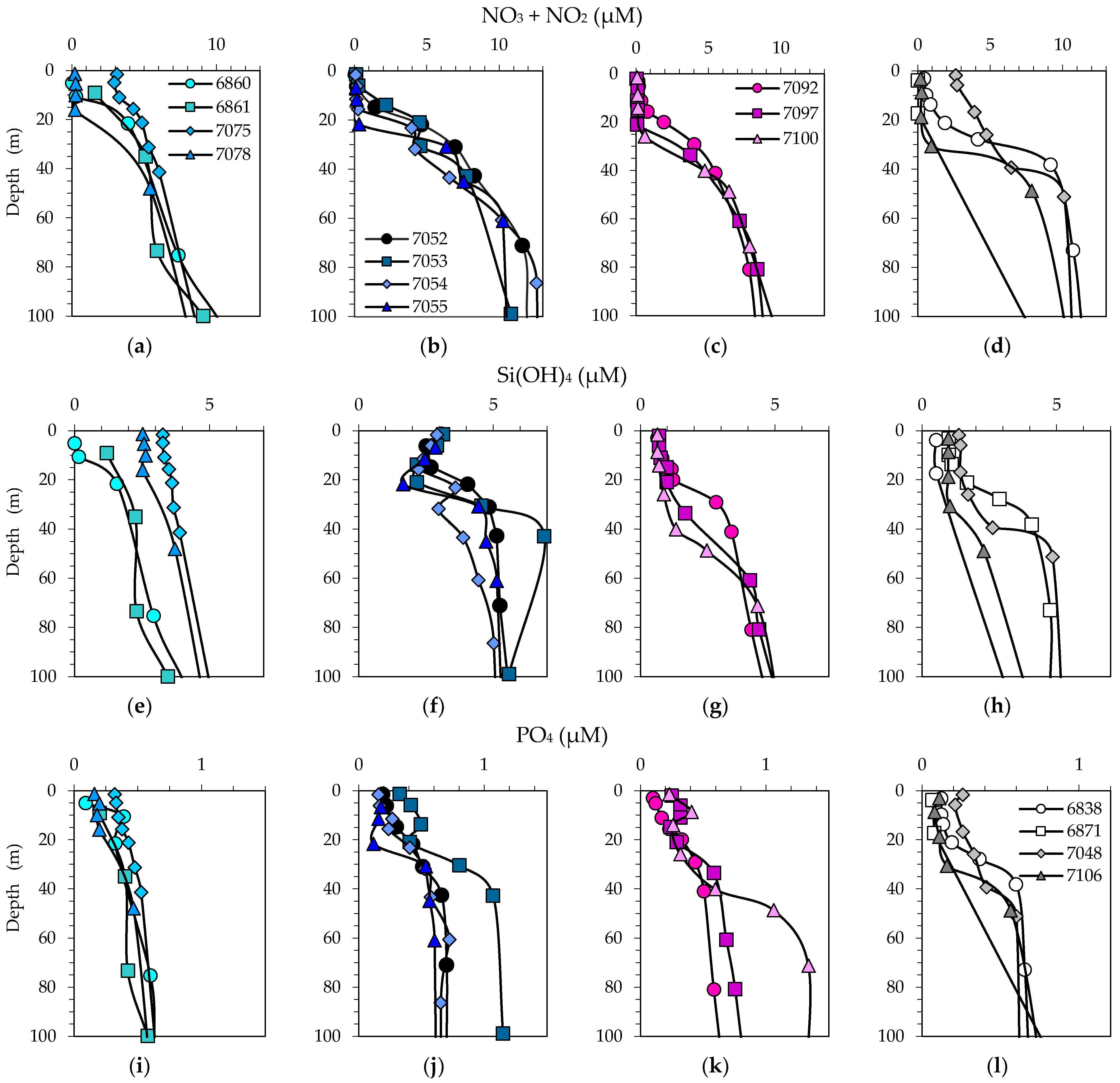
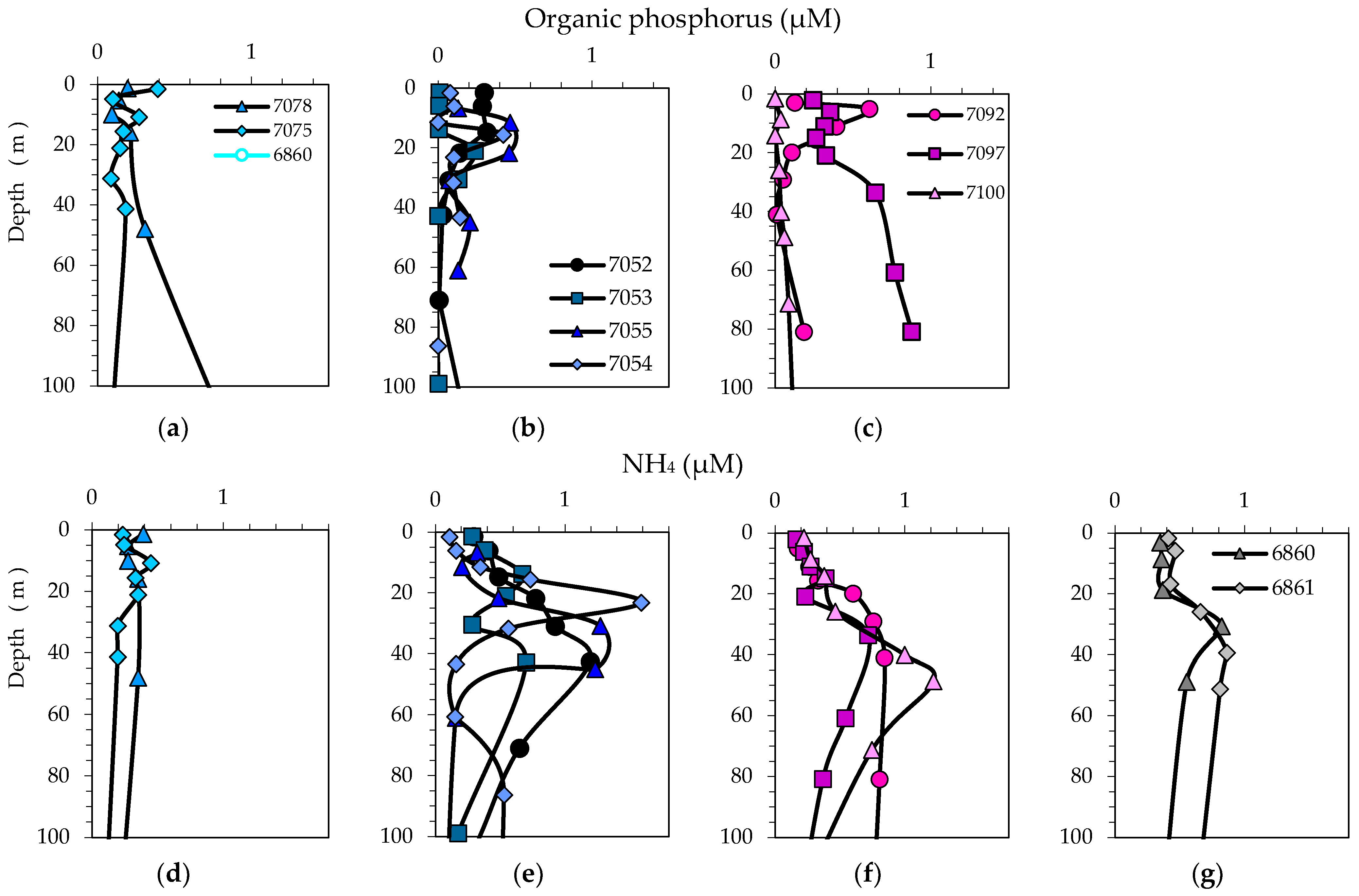
3.2. Physical, Optical and Chemical Conditions

The depth of the SML in the MIZ varied from 1 to 4 m in the Nansen Basin and in the Greenland Sea, from 7 to 11 m in the Barents Sea and reached 15–16 m at stations remote from the MIZ in the Norwegian and Barents Seas. At st. 7106 only, the SML extended by 35 m. In the Greenland Sea, the intrusion of PW into warmer AW created specific hydrological conditions in which “fingers” of PW were detected at different depths: a narrower cold core at depths of 15–40 m at sts. 7054 and 7055 (Figure 2). In the northern Barents Sea (Kvitøya Trough), the salinity stratification at st. 7092 was relatively weak (Δσ 0.9 kg∙m−3), allowing mixing. This corresponds to the low sea ice concentration in satellite images (Figure 1 (area IV)). Near the Mohns Ridge (Norwegian Sea), thermal stratification was disrupted (Δσ 0.4 kg∙m−3 in 2021). In 2020, the SML warmed more: TSML 9.8 vs. 8.1 °C in the Norwegian Sea and 9.4 vs. 8.0 °C in the southern Barents Sea.
The underwater light level was highest in the Nansen Basen at st. 7075, where the compensation irradiance (0.4 mol quanta∙m−2∙day−1 [7,9,38,39]) reached a depth of 44 m (Figure 3). The EGC contained water of polar origin and the zone of net phytoplankton growth was also much deeper (33–38 m). At other stations located in the MIZ, this boundary varied at depths from 25 to 31 m. The light conditions for photosynthesis were least favorable at st. 6871 (18 m) in the southern Barents Sea, where the thermal stratification was stronger (Δσ 1.1 kg∙m−3) than at st. 7106 (Δσ 0.6 kg∙m−3). The most transparent waters among the southern areas were at st. 7048 (34 m) in the Norwegian Sea.
A distinctive feature at the stations during the tests carried out in August 2021 in the MIZ of the Nansen Basin and Greenland Sea was the high concentrations of Si(OH)4 (>2 μM) in the SML, indicating non-intensive diatom growth (Figure 4). In 2020, low levels of Si(OH)4 corresponded the growth of silicate-consuming phytoplankton within the Zeu. 43% of PP variability and 41% of the Chl a concentration in the >10 μm phytoplankton group were explained by Si(OH)4 (Table S1). NO3 concentrations were substantially depleted (<0.5 μM) within the MIZ during both study periods, with the exception of st. 6861 and st. 7075 (1–3 μM). The PO4 concentration varied from 0.1 to 0.4 μM. In the Norwegian Sea, nitrogen supply to the Zeu (NO3 ~3 μM at st. 6838) may be a result of the interaction of currents over the underwater ridge area. In the southern Barents Sea (st. 6871), under the influence of relatively strong thermal stratification, the NO3 concentration reached analytical zero and the PO4 concentration decreased below the limit value (0.06 μM). The deep maximum of the NH4 concentrations was observed at different depths below the halocline and was present in all seas except for at st. 7075 in the Nansen Basin (Figure 5). The highest concentrations were measured in the MIZ of the Greenland and Barents Seas (1.2–1.6 μM). These NH4 concentrations corresponded to the maximum of the fluorescence signal (R2 = 0.36). In contrast, organic phosphorus was mainly concentrated in the SML (up to 0.4–0.6 μM). The Barents Sea MIZ was distinguished by a local increase in phosphorus concentration at the Zeu boundary: organic at st. 7097 (up to 0.9 μM) and inorganic at st. 7100 (up to 1.3 μM).

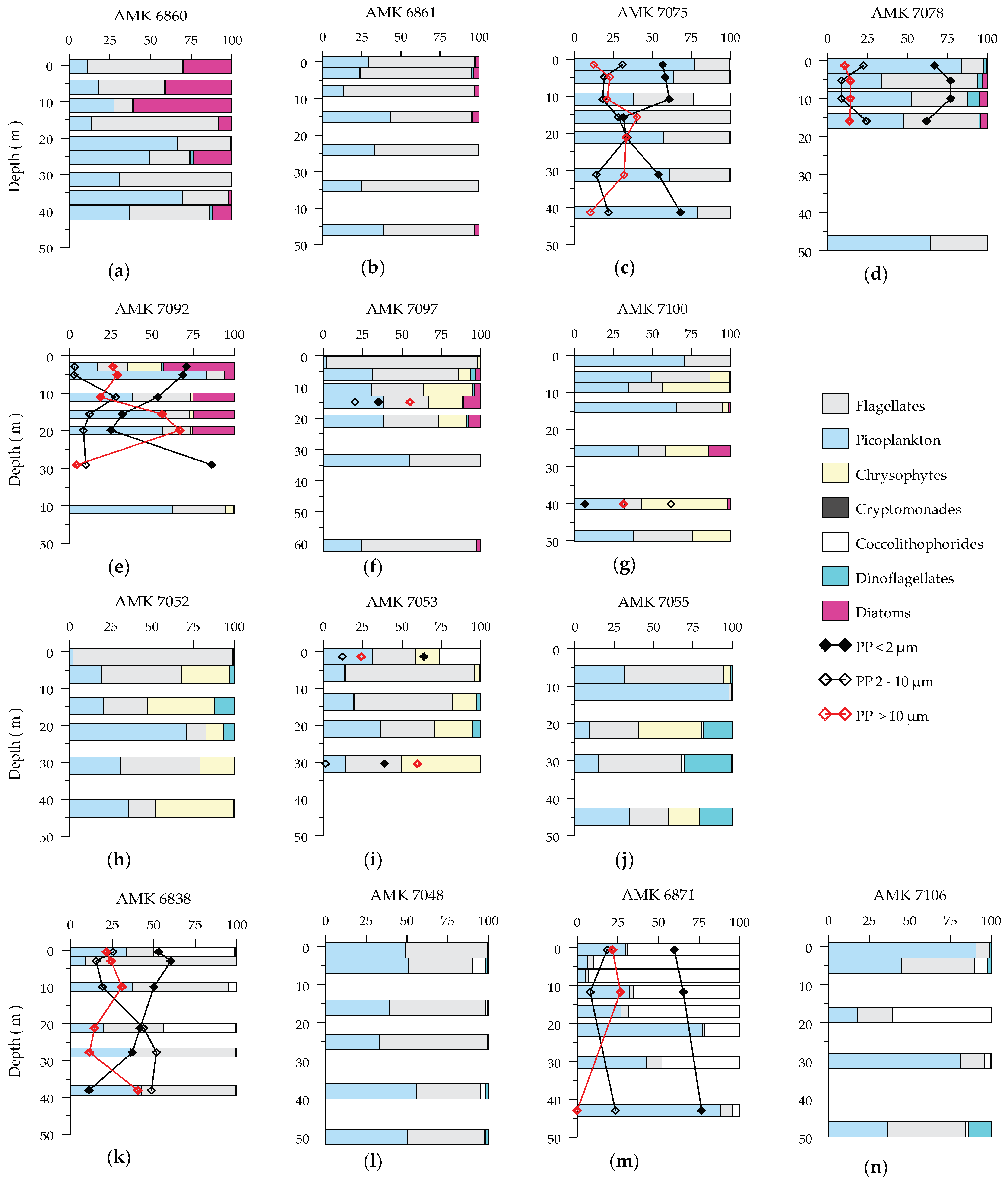
3.3. Phytoplankton Composition

The composition of diatoms at stations within the MIZ varied; low concentrations of Si(OH)4 were observed in the Zeu (Table S2). In the Nansen Basin, the large diatom Porosira glacialis accounted for the majority of PB above the halocline at the stage of peak bloom [40,41]. The Thalassiosira spp. T. gravida, T. nordenskioeldii and T. rotula were dominant at most depths in the Kvitøya Trough in the northern Barents Sea (Figure 6). P. glacialis and Fossulaphycus arcticus (previously known as Fosulla arctica) also made up a considerable share of the PB and could indicate the presence of nutrients from local upwelling. East of Kvitøya Island, Thalassiosira cells were abundant at depths below 15–20 m, where nutrient availability was higher (Figure 4). Large heterotrophic dinoflagellates (Gyrodinium lacryma, Protoperidinium brevipes and P. islandicum) dominated in the SML, whereas small flagellates (4–8 µm; st. 7097) and P. pouchetti (st. 7100) reached high abundance at the base of Zeu. A feature of these two stations was also the presence of vegetative cells of Dictyocha speculum and Dictyocha speculum below the halocline. At all other stations, only chrysophyte spores were found.
At stations with relatively high concentrations of Si(OH)4 in the Nansen Basin, Rhizosolenia hebetata, a diatom living in symbiosis with diazotrophic cyanobacteria in the tropics, contributed significantly to the biomass [42,43,44,45,46]. Thalassiosira spp. were found only at the early stage of bloom. The composition of heterotrophic dinoflagellates in the SML was less diverse (Gyrodinium spp. and Gymnodinium wulffii). In the Greenland Sea, the halocline was dominated by the genus Gyrodinium and the mixotrophic Prorocentrum minimum. Large diatoms (Eucampia groenlandica, Fragilariopsis cylindrus, Thalassiosira spp., Rhizosolenia spp. and P. glacialis), numerous spores and cysts in single amounts were found in cold water intrusions.
During the bloom of Emiliania huxleyi (>106 cells·L−1) in the southern Barents Sea, the high species diversity of dinoflagellates (28 species) was observed in both 2020 and 2021 (sts. 6871 and 7106). However, in 2021, the bloom area of E. huxleyi was characterized by a low density of detached coccoliths (104–105 cells·L−1). Very low phytoplankton abundance was observed in the Norwegian Sea (sts. 6838 and 7048). In 2020, the coccolithophores Coccolithus pelagicus and E. huxleyi, the diatoms Chaetoceros borealis, R. styliformis and R. hebetata and the dinoflagellates Dinophysis spp., Gymnodinium spp. and G. lacryma were represented in the samples. In 2021, cells of C. pelagicus, C. borealis, Tripos spp. and Gymnodinium spp. were found.

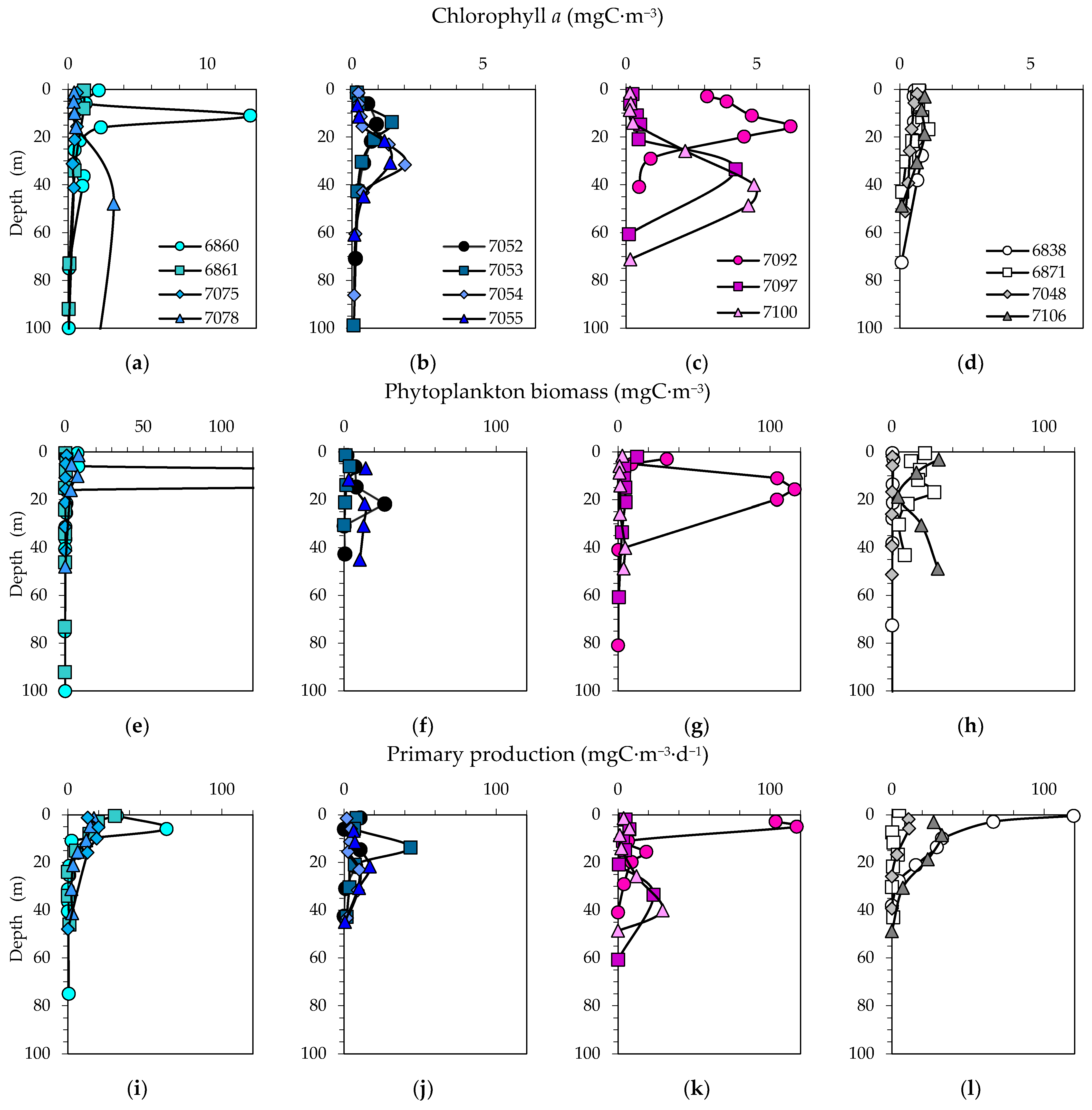
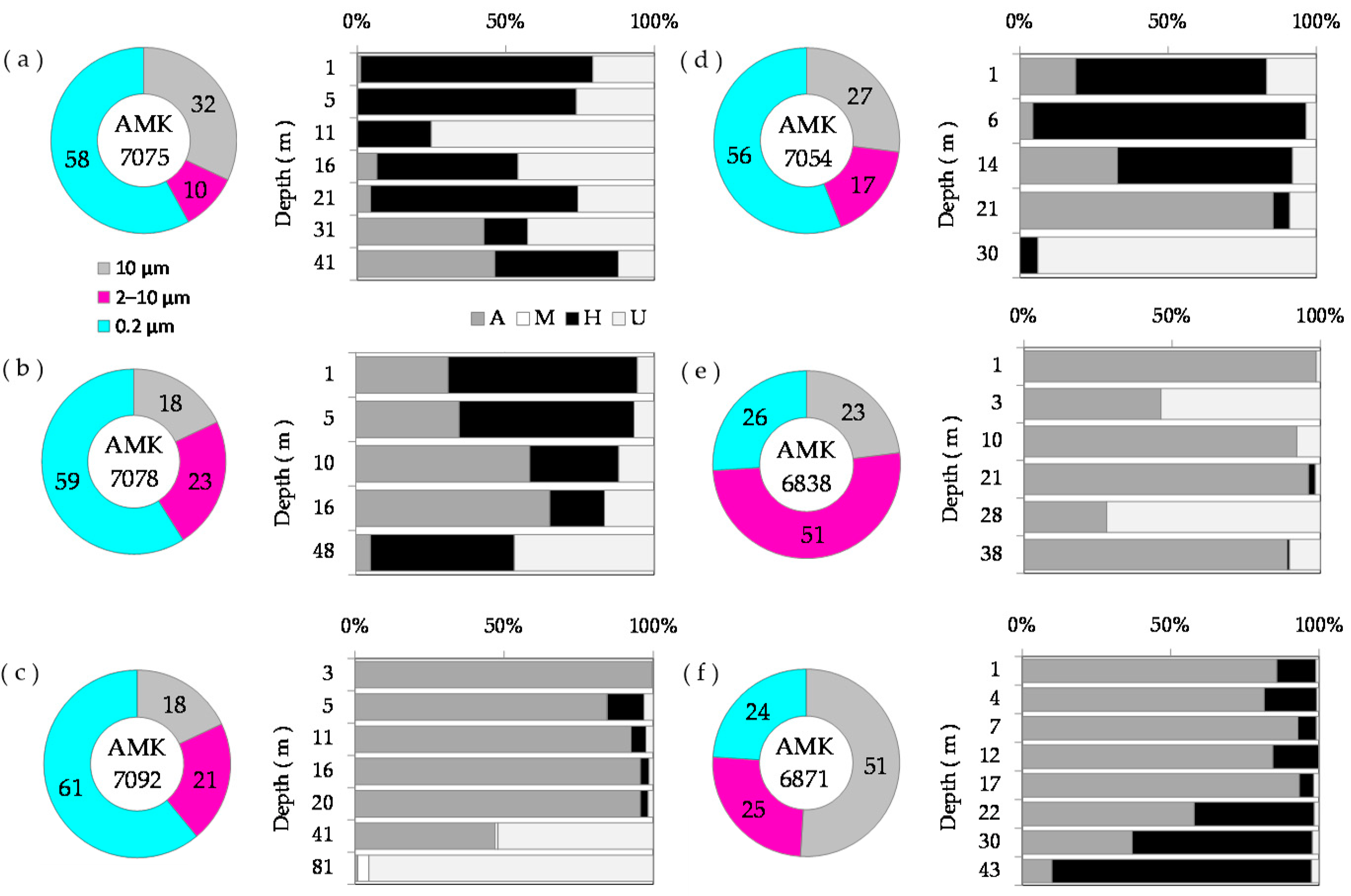
3.4. Size Distribution of Phytoplankton Carbon Biomass and Chlorophyll a

Phytoplankton of sizes > 10 µm contributed 80 ± 26% of the total PB in the MIZ but was less significant in the southern regions at different stages of the summer bloom (56 ± 30%). The maximum PB values were observed within the SML in the Kvitøya Trough (up to 112 mgC·m−3) and in the Nansen Basin (up to 799 mgC·m−3) near the edge of dense ice cover, as well as in the halocline layer (up to 27·mgC m−3) in the Greenland Sea (Figure 7). In other cases, the distribution of biomass across the Zeu was relatively constant (2.7 ± 4.8 mgC·m−3). In the southern Barents Sea, the PB was high (17 ± 9.3 and 20.2 ± 11.0 mgC·m−3 in 2020 and 2021, respectively), in contrast to the Norwegian Sea, where the PB was very low (0.5 ± 0.2 and 0.2 ± 0.1 mgC·m−3 in 2020 and 2021, respectively).
Analysis of the relationships between phytoplankton and environmental factors showed that their abundance influenced the organic phosphorus concentration and fluorescence signal. For both relationships the coefficient of determination was 0.36. Similar positive relationships with the indicated environmental factors were found for phytoplankton < 2 µm (R2 = 0.34 and R2 = 0.15, respectively). Diatom biomass explained 99% of the variation in autotrophic and total PB. Dinoflagellates were positively correlated with water temperature (R2 = 0.28) and NH4 concentration (R2 = 0.32). Chrysophyte abundance tended to increase with the concentrations of PO4 (R2 = 0.29) and NH4 (R2 = 0.29).
The biomass of heterotrophic species (mainly dinoflagellates) has always been high in the SML. In the Greenland Sea, this value reached 13 mgC·m−3. The biomass of these species increased with a decreasing NO3 concentration (R2 = 0.22).
Areas free of seasonal ice cover were also characterized by a relatively constant Chl a concentration of 0.6 ± 0.3 mg·m−3 in the Zeu. Within the MIZ, the maximum PB at depth was accompanied by a 2–8-fold increase in the Ch a concentration relative to the Chl a concentration in the surface layer. The deep maximum was observed in the Nansen Basin, with a peak value of 13.1 mg·m−3 (st. 6860). In the Kvitøya Trough, the deep Chl a maximum was less noticeable (st. 7092; peak value 6.3 mg·m−3). In the Greenland Sea, this maximus had a small magnitude (up to 2.2 mg·m−3).
To the east of Kvitøya Island (sts. 7097 and 7100) at the base of Zeu, the deep maximum of PB was not observed. However, the Chl a concentration increased from 17 to 32 times (up to 4.2–4.9 mg·m−3) in comparison with the surface value; 74 ± 19% of this concentration was Chl a in the > 10 µm phytoplankton group. In the Greenland Sea, the contribution of phytoplankton > 10 µm to Chl a was clearly low in PW “tongues” in the absence of settled diatom cells (the Chl a peak value is relatively low). In the Nansen Basin in 2021, more than half of the Chl a (61 ± 11%) was found in cells < 2 µm in size. Thus, the total Chl a content was higher in the Zeu at stations dominated by diatoms (42–118 mg·m−2) and relatively low (19–29 to 17–21 mg·m−2) in the MIZ and in regions free of seasonal ice cover where their share was low.
In general, the share of phaeophytin a in the total concentration of Chl a and the amount of phaeophytin a increases with increasing depth, as the passage of Chl a through the digestive tract of zooplankton favors the formation of pheophytin a. Similar profiles in the Greenland Sea indicate a similar phenomenon at these stations.
Within the MIZ, the deep fluorescence signal increased more strongly than the increase in Chl a concentration at the depth of its concentration maximum (up to 100–170 times), which is associated with a change in the pigment composition. The strongest relationships between the fluorescence and Chl a concentration were obtained for the <2 and 2–10 µm groups. The strong relationship (R2 = 0.52) between fluorescence and chrysophyte abundance is most likely a coincidence, as this group was represented predominantly by spores. On the other hand, the strongest signal peaks were observed in the northern Barents Sea, where chrysophytes were active. The signal intensity increased by 28% with increasing temperature and by 27% with increasing salinity.

3.5. Primary Production and Grouping of Stations in Relation to Bloom Study

Regarding nutrient depletion, the sts. 7075 (TSML −1.62 °C) and 6861 (TSML −1.44 °C) represented the early bloom stage due to the elevated NO3 concentrations. Among the remaining stations in the MIZ, the conditions at three of them (sts. 6860, 7078 and 7092; TSML from −1.49 °C to −0.11 °C) corresponded to the bloom peak stage due to the high values of PP and Chl a above the halocline, whereas the conditions at the rest of the stations (sts. 7052–7055, 7097, 7100; 0.51–2.82 °C) corresponded to the advanced phase of the bloom or the late stage of the bloom due to the occurrence of deep Chl a maximums and PP at depths from 25 to 40 m. The conditions in the areas free of seasonal ice cover corresponded to different stages of the summer phytoplankton bloom: bloom peak with high PP (sts. 6838 and 7106) and pre-bloom (st. 7048) or bloom end with extremely low PP (st. 6871).
Surprisingly, similar values for integrated PP at the peak bloom stage in 2020 and 2021 were observed in the Nansen Basin: 462 and 469 mgC·m−2·d−1. In the Greenland Sea, PP reached 618 mgC·m−2·d−1. In the northern Barents Sea (st. 7092), at the peak bloom stage, the PP was much higher than in the Nansen Basin (1109 mgC·m−2·d−1). This value was comparable with the PP of the summer maximum in the Norwegian Sea (1002 mgC·m−2·d−1). In 2021, the PP at this station was an order of magnitude lower (160 mgC·m−2·d−1). In the southern Barents Sea, despite the high PB, the PP did not exceed 45 mgC·m−2·d−1 in 2020 and reached 679 mgC·m−2·d−1 in 2021. This corresponded to a very strong nutrient depletion in the Zeu in 2020.

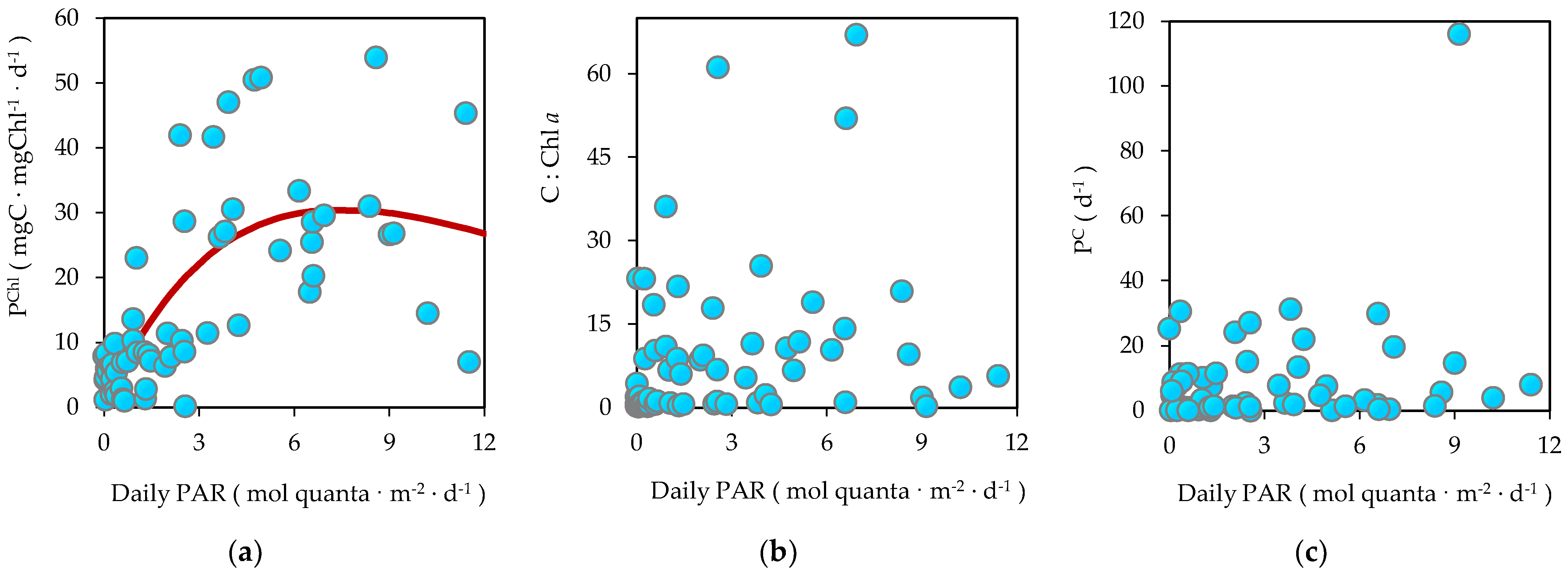
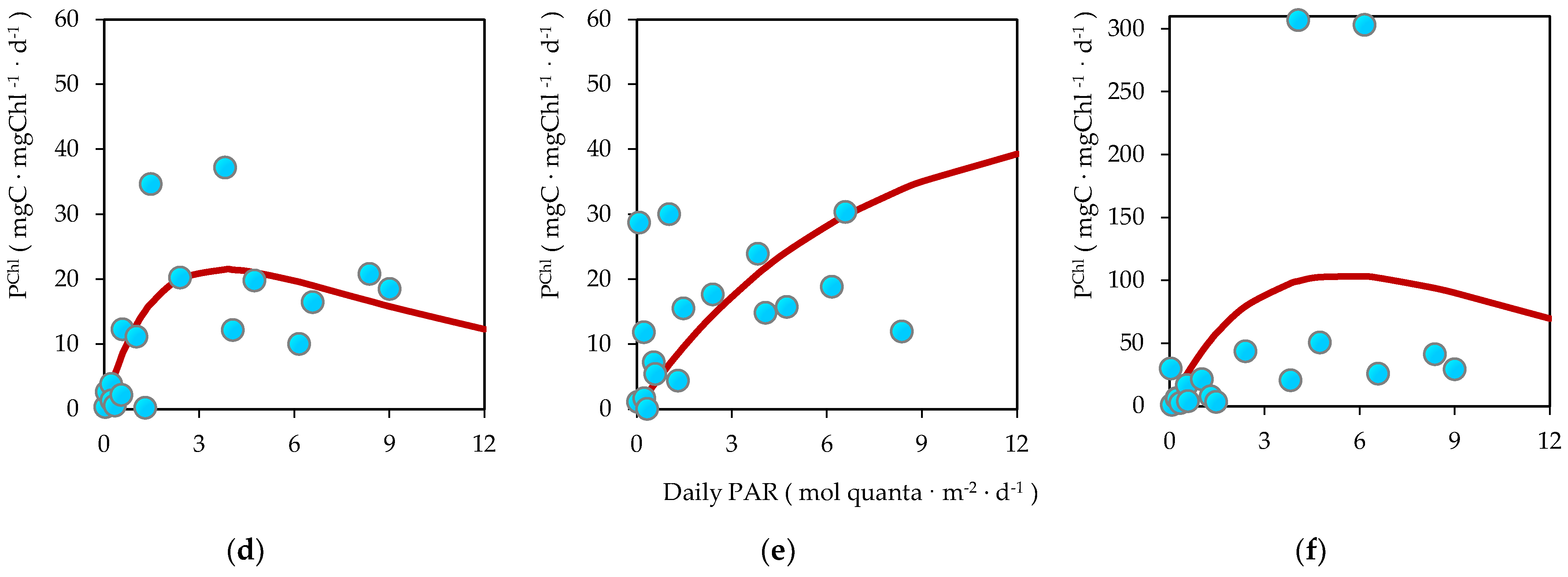
3.6. Biomass-Specific Carbon Assimilation

The acclimation of phytoplankton to different light conditions explains the weak relationship of the ratio of carbon (C) biomass to Chl a concentration (C:Chl a) with PAR within the MIZ (Figure 8). During the bloom peak stage, the C:Chl a ratio (up to 22–61) increased as a result of PB accumulation over the halocline. At the stage of bloom decline, high values of the ratio (up to 52–67) were observed in the SML. The highest C:Chl a ratio (21 ± 31, up to 101–126 in the SML) was observed in the > 10 µm phytoplankton group. Extremely low ratio values (0.4 ± 0.3) for phytoplankton acclimated to low light were observed at the early bloom stage. In addition to the light conditions, the C:Chl a ratio is sensitive to nutrient concentrations. In the southern regions of the European Arctic, the average C:Chl a ratio was 0.9 ± 0.5 and 33 ± 24 in the Norwegian and Barents Seas, respectively, which have a good supply of nutrients and severe resource deficiency, respectively.
The rates of biomass turnover in the MIZ were also independent of the daily PAR. The PC values ranged from 0.1 to 31 (8 ± 9) d−1 in the SML and appeared to increase with early-stage blooms. Unrealistically high PC values (13–14282 d−1) were obtained for phytoplankton < 2 µm in size. The PC of phytoplankton > 10 µm in size averaged 5 ± 12 d−1 in Zeu, whereas phytoplankton 2–10 µm in size averaged 12 ± 11 d−1. In contrast, the PChl was strongly dependent on irradiance, the nature of which was described by a non-linear photosynthesis–irradiance model in the presence of photoinhibition. For the data set from all stations in the MIZ plotted together, the maximum for photosynthesis reached 30 mgC·mgChl−1·d−1. Phytoplankton < 2 µm in size had the highest maximum PChl value (104 mgC·mgChl−1·d−1), and the lowest value was obtained for phytoplankton > 10 µm in size (22 mgC·mgChl−1·d−1). The corresponding daily irradiance optimum for these groups was 3.8 and 5.5 mol quanta·m−2·d−1, respectively. The lowest saturating light intensity was obtained for phytoplankton < 2 µm in size (1.2 mol quanta·m−2·d−1). Photoinhibition in this group potentially started at a high light intensity of 11.5 mol quanta·m−2·d−1, which was only achieved in the Greenland Sea on some days of the study.
The maximal value of PChl for total PB varied with the bloom phase: at the early stage the PChl was up to 29 mgC·mg·chl−1·d−1 and reached 47–51 mgC·mg·chl−1·d−1 at the peak and late stages of the bloom. This may reflect the increase in regenerated PP during the ice melt period. For example, the maximum value of PChl increased from 30 mgC·mg·chl−1·d−1 at the early stage to 51 mgC·mg·chl−1·d−1 at the stage of peak bloom in the Nansen Basin and to 307 mgC·mg·chl−1·d−1 during the peak bloom at the station in the Kvitøya Trough. Conversely, the maximum value of PChl for phytoplankton > 10 µm in size decreased from 37 mgC·mg·chl−1·d−1 at the early stage to 12 mgC·mg·chl−1·d−1 at the stages of peak bloom, which was consistent with increased nutrient limitation. In the southern regions studied in 2020, a high maximum value of PChl was recorded during the period of maximum activity of the ecosystem in the Norwegian Sea (125 mgC·mg·chl−1·d−1), and a very low PChl value (9 mgC·mg·chl−1·d−1) was observed in the Barents Sea during the termination of E. huxleyi growth. In 2021, the photosynthetic rates were 20 and 40 mgC·mg·chl−1·d−1, respectively.

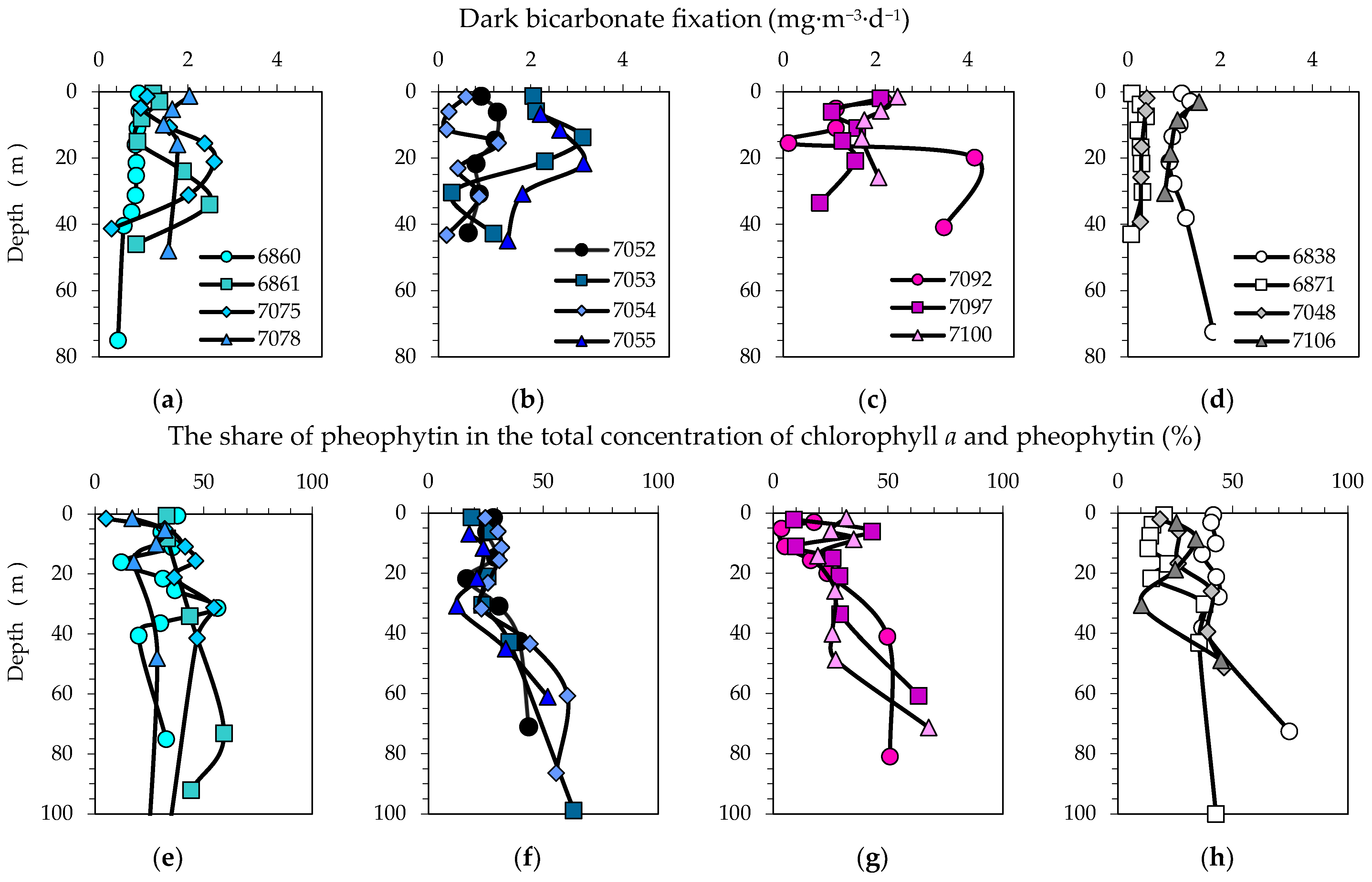
3.7. Bicarbonate Uptake in the Dark

Dark carbon fixation (DCF) is relevant to a wide range of metabolic groups (heterotrophs, chemoautotrophs and phototrophs capable of maintaining C fixation in the dark). Using data from the size-fractioned samples, we compared the share of inorganic C fixed by different size groups of microorganisms with the total assimilated C in the dark. In the MIZ, the share of plankton < 2 µm in size in DCF was relatively constant, ranging from 56 to 61% (Figure 9). This means that bicarbonate uptake in the dark may be dominated by chemotrophs or heterotrophic bacteria. This is consistent with the low availability of labile C in the MIZ. The share of nanoplankton (2–10 µm in size) in DCF tended to increase as it approached the peak-bloom in the MIZ, as well as in the southern regions where the peak-bloom situation was observed. In contrast, the content of the >10 µm group in DCF was increased at the early bloom stage and at the late bloom stage. This may reflect the high share of heterotrophs in the >10 µm group (36–76%) during these periods or other factors related to the phase of the phytoplankton bloom.
To avoid the potential effect of phototrophs as much as possible, we applied a correction to the measured rates by using the share of plankton < 2 µm in size in DCF (if the fractionalization of sample was not performed). The calculated rates of DCF ranged from 0.09 to 4.17 mgC·m−2·d−1. Two peaks characterized the vertical profiles of DCF—at the surface and in the halocline in the Barents Sea (Figure 10). In the Greenland Sea, the peaks were observed at or slightly below the halocline. However, at the peak-bloom stations in the Nansen Basin, the DCF values were distributed monotonically with depth. The temperature did not explain the variability in bicarbonate uptake in the dark with depth.
A relationship between both PP and dissolved organic phosphorous and DCF was not found. Comparing the rates of DCF above and below the halocline with biotic and abiotic factors, we found only a weak relationship between DCF and dissolved organic phosphorous in samples from the overlying halocline. Here, the dissolved organic phosphorous concentrations explained 27% of the DCF variability. The coefficients of determination in different fractions were highest for almost all biological parameters calculated for the 2–10 µm group (Table S1). This can be interpreted as the active feeding of bacteria and small phytoplankton in this group.

4. Discussion

4.1. Size Distribution of Phytoplankton Chlorophyll a, Biomass and Primary Production Relative to Previous Studies

The data obtained are close to the available published data for the northern Barents Sea and the Nansen Basin (from 75°30′ to 82°25′ N), where in May–July 2003–2005 the integrated PP reached 1475 mgC·m−2·d−1 and the maximum concentration of Chl a was 13 mgC·m−3 [48]. Our estimates of the total Chl a concentrations were lower than in the cited paper (up to 588 mg·m−2), partly because the authors performed calculations for a greater depth, which exceeded the real depth of Zeu. Other studies [49,50,51] report values for the Chl a concentration of < 200 mg·m−2, which also exceed the above estimates. In the northern Greenland Sea (the Fram Strait area) during May–July 1984–1985, the mean PP value was 426 mg·m−2 and the Chl a concentrations ranged from 87 to 185 mg·m−2. All these studies were conducted until early August and occurred during the start of the first phytoplankton bloom of the year in the MIZ dominated by diatom algae.
In previous periods, the contribution of phytoplankton > 10 μm in size to the total Chl a concentration was as high as 81% and the contribution to the integrated PP was 69% [48]. Our estimates of group contributions to the Chl a concentration (61.1–84.3%) at diatom bloom stations in the MIZ are consistent with the published data. However, in contrast to previous studies, the contribution of phytoplankton > 10 μm in size to the integrated PP did not exceed 34%. These differences reflect the higher Chl a concentrations in the cells, which is characteristic of phytoplankton adapted to low light levels, primarily diatoms [52].
The dominance of phytoplankton > 10 µm in size during the spring bloom is due to the high growth rate of diatoms. The concentration of nutrients allows them to grow faster than other cells in the environment [53,54,55]. When diatom growth is limited by NO3 and Si(OH)4, sufficient nutrients are maintained in the Zeu to allow dinoflagellates to grow successfully [56]. During our studies in the Greenland Sea, the conditions were favorable for this phenomenon: a stratified layer with low salinity, where cysts had more time for proliferation. The most abundant species, P. minimum, is usually dominant in brackish eutrophic estuaries [57,58]. This species develops when cells encounter high nutrient concentrations and increased light. The dominant phytoplankton groups were found to be more affected by meltwater input than by temperature in this area [59].
In situ measurements of PP samples deployed on a on buoy at sts. 6860 and 7054 allowed us to confirm the accuracy of the vertical distributions obtained at other stations by simulating the in situ conditions. In combination with synchronous measurements of the Chl a concentration and phytoplankton cell size, this also allowed us to understand the adequacy of the measured PP and hence of the biomass growth rates specific to Chl a and C. The latter reached very high values (up to 7.8 d−1) in situ, significantly exceeding the theoretical growth rates for low water temperatures [60,61]. A possible source of these discrepancies in our 14C uptake experiments may be an underestimation of the biomass of autotrophs < 2 µm in size, since we consider their production (biomass) and Chl a to be fully accounted for on filters with a pore size of 0.2 µm. When the PB growth rates of autotrophs > 10 μm in size are taken into account, it is still highly underestimated, up to 4–5 d−1 at advanced bloom stages and up to 51 d−1 at the early bloom stage in the Nansen Basin.
In terms of nutrient availability, this suggests that interaction with sharply contrasting meltwater in the MIZ leads to increased phytoplankton growth rates near the halocline. Permafrost meltwater, glacier outflows, coastal erosion and river runoff with elevated concentrations of micronutrients, silicates and stocks of organic matter containing element-binding ligands are thought to be the source of their input to lower latitudes through the “gateway to the Arctic” [62,63,64,65]. Macro- and microelement additions in the Arctic–Atlantic matter exchange zone in the Fram Strait increased phytoplankton growth intensity near Svalbard [66]. North of Svalbard, a tendency for a decrease in Si(OH)4 concentration was found [67]. Thus, high concentrations of sea ice in 2020 in the Nansen Basin could contribute not only to the accumulation of biomass in the halocline but also to the intensification of diatom blooms that provide phytoplankton with deficient elements [40,41]. In the area of Kvitøya Island, the content of terrigenous matter should have been higher, which could support the Thalassiosira bloom on the Barents Sea shelf as their bioavailability increased [63,68,69,70].
The strong dependence of chrysophytes on the environmental conditions and biological variables revealed in our studies forces us to pay attention to the dominant species in this group—autotrophic silicoflagellates Dictyocha speculum that are ~30 μm in size and mixotrophic Dinobryon balticum that are ~40 μm in size. They often form blooms in the spring in transactional areas, where an interaction between brackish and saline waters occurs [71,72]. The optimum temperature for their development is above 10 °C. Thus, the intensive growth in the MIZ may be a sign of ongoing climate change.
A two-dimensional vertical model cannot be assumed to account for all phytoplankton growth factors within the MIZ, where the meltwater layer is highly displaced relative to the underlying layer. In 2020, based on the concentration of Si(OH)4 at a 100 m depth (where biological consumption is low), the biomass of P. glacialis could be about 221 mgC·m−3 and the calculated PP (442 mgC·m−3·d−1) was comparable to the measured value [73]. The detection of E. huxleyi cells in appreciable concentrations in the halocline in the Nansen Basin in 2021 (where the PC reached 51 d−1) indicates a dramatic change in the biomass in the Zeu due to advection. In the Western Spitsbergen Current, in situ production of biomass can be 5–50 times lower than the advective production [74]. Thus, our data confirm the published data showing that the contribution of advective PB is very large. Obviously, this is why we obtained such high estimates for the growth rates at halocline depth in the MIZ.

4.2. Phytoplankton Bloom Dominated by Small Phytoplankton in the MIZ

The dominance of small cells at the highest latitudes is confirmed by the results of optical observations at autonomous stations [8,9,75,76]. In the central AO (~83–88 N), which received meltwater in August 2010, the abundance of phytoplankton < 2 μm in size varied from 1.58 × 10⁶ to 9.47 × 10⁶ cells·L−1 and the contribution to the total chlorophyll a concentration ranged from 44 to 80% [77]. Our data on the contribution of phytoplankton < 2 μm in size to the Chl a concentration in the Nansen Basin in 2021 are in good agreement with the results of the published data. The measured abundance values were much lower (about 104–105 cells·L−1) because we did not use methods that allow counting the number of small cells in the total volume (flow cytometry or counting in an epifluorescence microscope).
Small cells are characterized by a low ratio of cell surface area to cell volume and an increased microcellular nitrogen content, which is an advantage under conditions of nutrient limitation [55,78,79]. They account for up to 90% of phototrophic biomass in oligotrophic areas. However, at the early bloom stage, nutrients do not limit phytoplankton growth. Therefore, a possible reason for the dominance of small cells in the Nansen Basin in August 2021 could be the variable light regime under conditions of weakened ice cover and intense mixing, as evidenced by either the complete absence or deep location of the Chl a maximum. At critical PAR levels, the high photosynthetic efficiency of phytoplankton < 2 μm in size is facilitated by the large light absorption capacity of the Chl a unit in the cell (in the absence of the “package effect”) [80,81]. Arctic diatoms require time to adapt to the changing light conditions, which occurs faster with gradual increases in light than with rapid transitions from a strong to weak light level [7,52,82]. Therefore, a variable light regime among drifting ice is less favorable for them.
According to Zhang et al. [77], all major taxonomic divisions of phytoplankton were represented in the < 2 μm group in the North Pole area. This distinguishes this group from large phytoplankton, where Chlorophyta and Phaeocystis dominate in terms of cell number. Diatoms (Chaetoceros, Thalassiosira, Actinocyclus, Pleurosigma and Navicula) accounted for 2 to 80% of the total Chl a concentration. It is possible that in the Nansen Basin in 2021, diatoms < 2 μm in size dominated, for which the growth limiting factors of large cells were irrelevant. Silicate production (= silicate depletion rate) was more dependent on cell volume than the growth rate or frustule thickness. However, on the scale of days, the influential role of the growth rate increases [83]. Diatoms with smaller cells are expected to have slower growth rates than diatoms with larger cells because they develop in diatom-inhospitable conditions where silicate uptake is reduced [67].
Finally, the different ecology of species largely explains the wide range of light levels that are optimal for photosynthesis in phytoplankton < 2 μm in size, which we revealed by fitting field measurements to the theoretical model. It can be assumed that the low threshold of photosynthetic light saturation is related to diatoms (1.2 mol quanta·m−2·d−1), which, like the large species, contributed to the formation of the deep Chl a maximum at the base of the Zeu. In contrast, the lack of photoinhibition at PAR > 5.6 mol quanta·m−2·d−1 obtained for phytoplankton > 10 µm in size was associated with a change in the composition of the community of small cells and the occurrence of species inhabiting environments with high light intensities, such as the unicellular green algae Micromonas (group Mamiellophyceae) or Arctic endemic cyanobacteria [19,21,84,85]. It has recently been shown that these algae can be adapted to a variety of ecological niches [86].

4.3. The Contribution Mixotrophs and Zooplankton to Ecosystem Dynamic

Nanophytoplankton is the most effective primary producer because it combines the advantages of both larger and smaller phytoplankton [55,87]. This group appears to have compromised on cell size and nutrient availability.
Phaeocystis is a representative of cold-water communities living at temperatures < 6 °C [88]. Some reviews consider Phaeocystis blooms as the second annual maximum of phytoplankton development in the Arctic. However, simultaneous co-dominance of diatoms is also often reported [7,49,50]. This is consistent with data from the northern Barents Sea, where we observed co-dominance with diatoms in cold water at temperatures of around −1 °C. Haptophytes are often mixotrophic and dominate the microbial food web. Phaeocystis phagotrophy was proved only for some species, although previously viable cells of P. pouchetii were found under polar night conditions [88]. According to indirect data, heterotroph activity increases in depths where Phaeocystis vegetated during our studies.
The coexistence of classical and microbial food webs was observed in the Kongsfjord of the Svalbard all year round and in the MIZ of the central Barents Sea in summer [89,90]. In the northernmost regions, similar conditions seem to occur. Calanus glacialis is widely distributed in cold PW of the northern Barents Sea and probably has a two-year life cycle in ice-covered PW [91,92]. During our studies, the abundance of Chaetoceros spp. could be controlled by zooplankton at stations of bloom decline, where signs of heterotrophic activity were obtained. Thalassiosira can resist grazing and sedimentation by forming chains [93,94]. In a previous study [17], the high particulate silica content in the trapped samples was explained by the presence of chain-forming species of Thalassiosira in the northwestern Barents Sea.
Many researchers have highlighted the significant role of nanoflagellates in the PP of Arctic seas [89,95]. The reduced and comparable concentrations of Chl a in phytoplankton of 2–10 μm in size within the MIZ indicate a high share of heterotrophs in nanoplankton and explain the low biomass and high level of PP and DCF of the 2–10 μm group in our studies. A high abundance of mixotrophic ciliates may also be responsible for the reduced Chl a concentration in phytoplankton 2–10 μm in size. Ciliates, such as Mesodinium rubrum (Myrionecta rubra), Laboea strobila and various Pseudotontonia, Spirotontonia and Strombidium use plastids sequestered from chlorophytes, cryptophytes, haptophytes and stramenopiles to obtain energy and metabolic products from photosynthesis [96,97,98,99].
In both years at the studied stations in the Barents and Norwegian Seas, located at approximately the same latitude (72.4 and 73.4° N), the PP differed by two times and the PB by two–three orders of magnitude. At similar temperatures in the SML during each study period, the initial supply of nutrients and zooplankton grazing may influence the PP within the Zeu. The physical, chemical and biological data from the stations in the Norwegian Sea obviously indicate upwelling of water from the deepest layers under the fluctuation of currents responding to underwater rise. Cyclonic eddies also prevail on the eastern slope of the ridge and can contribute to the supply of nutrients to the Zeu [100]. This may lead to increased PP level, which is consistent with previous estimates of PP in the area [101]. According to research carried out by the Working Group on Integrated Ecosystem Assessments for the Norwegian Sea, the summertime biomass of zooplankton is relatively high in the northeastern area of the Mohns Ridge [102] and has reached 12–14 g∙m−2 in recent years [103]. Export production in the summer period is nearly absent. Fluxes of organic matter to the seabed only increase in the autumn [104,105,106]. This means that zooplankton from the upper water layer was a potential active feeder and controlled the PB in the ridge area and in the Norwegian Sea as a whole [107].
The poleward expansion of E. huxleyi in the European Arctic is one of the most pronounced traces of ongoing climate changes [108,109,110]. The expansion of E. huxleyi is limited by a water temperature of 4 °C. Low salinity is also an unfavorable factor for the development of coccolithophores. Thus, in the Baltic Sea, their abundance decreases rapidly along the salinity gradient and the ecological niche is occupied by other haptophytes in the summer [33,111,112]. The reasons for the wide distribution of E. huxleyi in the southern Barents Sea have not been fully elucidated [108,109]. Low NO3 concentrations in the North Sea have been found to be associated with bloom formation rather than PO4 [113]. It has also been reported [113,114] that E. huxleyi blooms occur at shallow SML depths and high surface PAR levels. In the bloom area, E. huxleyi can provide >30% of the organic carbon fixation [115]. In mixed communities, their cells usually account for 5–40% of the PB. Our results are consistent with the data, according to which a decrease in the PP and Chl a values was observed in bloom patches compared with the surrounding waters (three-fold decrease in PP) [113]. The high irradiance level affects carbon fixation in organic compounds and the biochemical composition of organic matter newly synthesized by coccolithophores. The low values of PP measured in 2020 in the advanced bloom stage may be characteristic of the study area of the southern Barents Sea. Their low values were a result of an atypically high contribution to the PB (from 22 to 90% of the PB within Zeu) (st. 6871). In 2021, st. 7016, contrary to our predictions, was outside the E. huxleyi bloom area due to a cloudy sky during the sampling period (actual satellite data not available). The remaining species indicated in this area were the primary producers that resulted in the high PP level. Among the > 10 µm phytoplankton group, autotrophic dinoflagellates prevailed in the area in 2021. In contrast, heterotrophic dinoflagellates were the most abundant in the E. huxleyi bloom area in 2020.
According to long-term observations during the period 1986–2020 [90], the zooplankton biomass was lower in the coastal and shallow bank waters of the Barents Sea. In the southern areas of the AW inflow in the west, zooplankton biomasses increased due to the growth of the second summer generation of Calanus finmarchicus. The presence of coccoliths may limit zooplankton grazing, which causes the relatively high PB in the southern Barents Sea [116,117]. However, recent mesocosm-based experiments have shown that the possession of coccoliths does not provide E. huxleyi effective protection from grazing [118]. In our analysis, when calculating the post-incubation carbon biomass, we considered phytoplankton cells that could potentially be consumed by zooplankton during incubation, as we did not remove zooplankton from the samples. In communities dominated by coccolithophorids, the PB was increased, which may indicate less intensive zooplankton feeding (compared with the Norwegian Sea).

4.4. Dark Bicarbonate Fixation as a Bacterial Heterotrophic Production Indicator

In this study, we found high rates of DCF corresponding to the same range as the bacterial heterotrophic production rates (0.09–153 mgC·m−3·d−1) commonly reported for the various freshwater and marine ecosystems [119,120,121,122,123]. It is the integrated DCF values within the MIZ (25–104 mgC·m−2·d−1) that are consistent with estimates of the integrated bacterial heterotrophic production (<30–170 mgC·m−2·d−1) in Kongsfjord (Western Svalbard) [87], where a combination of local glacial and freshwater runoff and AW inflow drives the environmental conditions.
Recent data show [37,87,119,120,121,122,123] that photosynthetic production of organic matter and bacterial heterotrophic production under oligotrophic conditions can be temporally disconnected at daily to seasonal scales. This may explain the weak correlation of DCF with most of the marine indices considered and the poor correspondence of DCF to the bloom stage in the MIZ. This is clearly demonstrated in the Nansen Basin, where the rates of DCF increased at the early-bloom stage when the opposite would be expected. In contrast, we obtained a weak correlation between DCF and dissolved organic phosphorous in the MIZ of the Barents Sea, where the rates of DCF increased. The observed differences can be explained by the fact that the dark uptake of bicarbonate is noticeably different among the Arctic heterotrophs, whose composition depends on many factors, including the quality and quantity of labile organic C [70,124]. Combining measurements of the incorporation of bicarbonate, leucine and thymidine into the bacterial biomass with data on the composition of microorganisms can provide a better understanding of the biogeochemical role of bacteria in the MIZ.

5. Conclusions

We observed different situations in the MIZ in August 2020 and 2021. In 2020, the bloom of the centric diatom P. glacialis developed on the halocline in the Nansen Basin where there was dense ice cover with a high total PB in the Zeu (2.1 gC·m−2). In 2021, when ice cover was sparse, low-gradient stratification favored the rapid sedimentation of large cells of Rhizosolenia (0.2 gC·m−2). The phytoplankton was dominated by a fraction of small phytoplankton < 2 µm in size. In the northern Barents Sea, the fields of shallow ice were dominated by Thalassiosira, which was capable of resisting a rapid sinking (1.9 gC·m−2). Phaeocystis and small flagellates were important in this bloom. Under increased light intensity conditions in the Greenland Sea, the ecosystem of the MIZ was based on mixotrophic–heterotrophic dinoflagellates dominated by the eutrophic water dinoflagellate P. minimum (0.4 gC·m−2).
In all conditions considered, phytoplankton < 2 µm in size formed the basis of the particulate PP (47–69%) and phytoplankton > 10 μm in size prevailed in the total PB (88–99%). The trophic interactions between classical and microbial food webs in MIZ seems to be weakened, and the sites of growth and accumulation of phytoplankton > 10 µm in size were highly spatially disconnected. From the early stage to the late stage of the bloom, the biomass-specific carbon fixation rate decreased, whereas the chlorophyll-specific carbon fixation rate increased. These rates reached their maximum values at depths with irradiance in the range of 3.5–5 mol quanta·m−2·d−1, which is optimal for the phytoplankton photosynthesis with sizes > 10 µm and <2 µm. In the late stage of the bloom, diatoms increased the Chl a content in cells at the base of the Zeu, where the biomass and activity of phytoplankton < 10 µm was also high (74% of the PB and 60% of the PP). In this case, the microbial food web, in addition to increasing nutrient concentrations, contributed to an increase in diatom production.
We found that the saturating light intensity for phytoplankton < 2 µm in size was the lowest among the selected size groups (1.2 mol quanta·m−2·d−1) and photoinhibition began at high light intensities (11.5 mol quanta·m−2·d−1). This means that the PP by small phytoplankton formed the basis of the total PP in the MIZ irrespective of the sea ice cover state. In contrast, phytoplankton > 10 µm in size responded to the light, stratification, and macro- and micronutrient concentrations that were related to the sea ice cover conditions.
At the stage of the peak bloom in the Nansen Basin, the remarkably close PP levels indicated the ecological flexibility of pelagic ecosystems in the European Arctic during global climate change; this flexibility allowed the PP to be maintained at maximum level. However, transformation of phytoplankton-based carbon cycle occurs as a result of adaptation of primary producers to changes in environmental conditions, the consequences of which are still poorly understood. Ice cover serves as one of the most important factors in switching the PP regime from the dominance of large phytoplankton to the dominance of small phytoplankton and the transition from the perturbed state to the balanced state under the influence of water column stratification and light conditions. In the Norwegian Sea and southern Barents Sea, we emphasized two possible summer scenarios for the northern parts of the European Arctic in case of continued ice cover reduction and surface water layer warming.

Supplementary Materials

The following supporting information can be downloaded at: https://www.mdpi.com/article/10.3390/jmse11112131/s1. Table S1: Linear regression analysis of the relationship between phytoplankton and environmental factors and the biological variables in the MIZ of the Nansen Basin and Barents and Greenland Seas; Table S2: Complex of dominant phytoplankton species.

Author Contributions

Conceptualization, E.K.; Methodology, E.K. and M.K.; Formal Analysis, E.K., M.K., L.P., I.R., D.G.; N.T., A.C., N.P., A.S. (Alexander Shchuka) and I.Z.; Data Curation, M.K. and D.G.; Writing—Original Draft Preparation, E.K.; Writing—Review and Editing, E.K., M.K. and I.R.; Visualization, E.K.; Supervision, N.P. and A.S. (Alexander Savvichev); Project Administration, M.K.; Funding Acquisition, M.K. All authors have read and agreed to the published version of the manuscript.

Funding

This research was carried out within the framework of the state assignment of Shirshov Institute of Oceanology, Russian Academy of Science (theme no. FMWE-2021-0006). Radiotracer studies were supported by the state assignment of the Winogradsky Institute of Microbiology, Research Center of Biotechnology of the Russian Academy of Sciences. PAR measurements and data processing were funded by the Russian Science Foundation (project no. 21-77-10059). The research cruise was carried out with the financial support of the Ministry of Science and Higher Education of the Russian Federation.

Institutional Review Board Statement

Not applicable.

Informed Consent Statement

Not applicable.

Data Availability Statement

The original material presented in the study is included in the manuscript and Supplementary Material; additional enquiries may be directed to the corresponding author.

Acknowledgments

We would like to thank the crew of the RV Akademik Mstislav Keldysh, Alexey Klyuvitkin, Alexander Novigatsky, Vladimir Artemiev, Anton Bulokhov, and Georgy Malafeev for the help with in situ measurements of primary production. We are also grateful to Alexander Khrapko for helping acquire the PAR data, Olga Netzvetaeva for the assistance in hydrochemical analyses processing. We acknowledge Vladimir Silkin for his help during the cruise and for valuable suggestions and feedback on the manuscript. We appreciate the constructive and insightful comments of the reviewers.

Conflicts of Interest

The authors declare no conflict of interest.

Nomenclature

AMKAkademik Mstislav Keldysh
Chl achlorophyll a
C:Chl acarbon-to-chlorophyll a ratio
CTDconductivity–temperature–depth
DCFdark carbon fixation rate
DPMdisintegrations per minute
MIZmarginal ice zone
PARphotosynthetically active radiation
PBphytoplankton carbon biomass
PChlchlorophyll-specific particulate primary production rate at individual depths
PCcarbon-specific particulate primary production rate at individual depths
PPparticulate primary production at individual depths
PSUpractical salinity unit
SMLsurface mixed layer depth
Zeueuphotic zone

References

  1. Kwok, R.; Rothrock, D.A. Decline in Arctic Sea ice thickness from submarine and ICES at records: 1958–2008. Geophys. Res. Lett. 2009, 36, L15501. [Google Scholar] [CrossRef]
  2. Polyakov, I.V.; Pnyushkov, A.V.; Alkire, M.B.; Ashik, I.M.; Baumann, T.M.; Carmack, E.C.; Goszczko, I.; Guthrie, J.; Ivanov, V.V.; Kanzow, T.; et al. Greater role for Atlantic inflows on sea-ice loss in the Eurasian Basin of the Arctic Ocean. Science 2017, 536, 285–291. [Google Scholar] [CrossRef] [PubMed]
  3. Arrigo, K.R.; van Dijken, G.L. Continued increases in Arctic Ocean primary production. Prog. Oceanogr. 2015, 136, 60–70. [Google Scholar] [CrossRef]
  4. Hill, V.; Ardyna, M.; Lee, S.H.; Varela, D.E. Decadal trends in phytoplankton production in the Pacific Arctic Region from 1950 to 2012. Deep. Sea Res. Pt. II 2018, 152, 82–94. [Google Scholar] [CrossRef]
  5. Dalpadado, P.; Arrigo, K.R.; van Dijken, G.L.; Skjoldal, H.R.; Bagøien, E.; Dolgov, A.V.; Prokopchuk, I.P.; Sperfeld, E. Climate effects on temporal and spatial dynamics of phytoplankton and zooplankton in the Barents Sea. Prog. Oceanogr. 2020, 185, 102320. [Google Scholar] [CrossRef]
  6. Lewis, K.M.; van Dijken, G.L.; Arrigo, K.R. Changes in phytoplankton concentration now drive increased Arctic Ocean primary production. Science 2020, 369, 198–202. [Google Scholar] [CrossRef]
  7. Ardyna, M.; Mundy, C.J.; Mayot, N.; Matthes, L.C.; Oziel, L.; Horvat, C.; Leu, E.; Assmy, P.; Hill, V.; Matrai, P.; et al. Under-Ice Phytoplankton Blooms: Shedding Light on the “Invisible” Part of Arctic Primary Production. Front. Mar. Sci. 2020, 7, 985. [Google Scholar] [CrossRef]
  8. Boles, E.; Provost, C.; Garçon, V.; Bertosio, C.; Athanase, M.; Koenig, Z.; Sennéchael, N. Under-ice phytoplankton blooms in the central Arctic Ocean: Insights from the first biogeochemical IAOOS platform drift in 2017. J. Geophys. Res. Oceans. 2020, 125, e2019JC015608. [Google Scholar] [CrossRef]
  9. Randelhoff, A.; Lacour, L.; Marec, C.; Leymarie, E.; Lagunas, J.; Xing, X.; Darnis, G.; Penkerc’h, C.; Sampei, M.; Fortier, L.; et al. Arctic mid-winter phytoplankton growth revealed by autonomous profilers. Sci. Adv. 2020, 6, eabc2678. [Google Scholar] [CrossRef]
  10. Falk-Petersen, S.; Hop, H.; Budgell, W.P.; Hegseth, E.N.; Korsnes, R.; Løyning, T.B.; Ørbæk, T.K.; Kawamura, T.; Shirasawa, K. Physical and ecological processes in the marginal ice zone of the northern Barents Sea during the summer melt periods. J. Mar. Syst. 2000, 27, 131–159. [Google Scholar] [CrossRef]
  11. Assmy, P.; Fernández-Méndez, M.; Duarte, P.; Meyer, A.; Randelhoff, A.; Mundy, C.J.; Olsen, L.M.; Kauko, H.M.; Bailey, A.; Chierici, M.; et al. Leads in Arctic pack ice enable early phytoplankton blooms below snow-covered sea ice. Sci. Rep. 2017, 7, 40850. [Google Scholar] [CrossRef]
  12. Strass, V.H.; Nöthig, E.M. Seasonal shifts in ice edge phytoplankton blooms in the Barents Sea related to the water column stability. Polar Biol. 1996, 16, 409–422. [Google Scholar] [CrossRef]
  13. Castellani, G.; Schaafsma, F.L.; Arndt, S.; Lange, B.A.; Peeken, I.; Ehrlich, J.; David, C.; Ricker, R.; Krumpen, T.; Hendricks, S.; et al. Large-scale variability of physical and biological sea-ice properties in polar oceans. Front. Mar. Sci. 2020, 7, 536. [Google Scholar] [CrossRef]
  14. Sakshaug, E.; Skjoldal, H.R. Life at the ice edge. Ambio 1989, 18, 60–67. [Google Scholar]
  15. Margalef, R. Life-forms of phytoplankton as survival alternatives in an unstable environment. Oceanol. Acta 1978, 1, 493–509. [Google Scholar]
  16. Falkowski, P.G.; Laws, E.A.; Barber, R.T.; Murray, J.W. Phytoplankton and their role in primary, new, and export production. In Ocean Biogeochemistry. Global Change—The IGBP Series; Fasham, M.J.R., Ed.; Springer: Berlin/Heidelberg, Germany, 2003; pp. 99–121. [Google Scholar]
  17. Krause, J.W.; Duarte, D.M.; Marquez, I.A.; Assmy, P.; Fernández-Méndez, M.; Wiedmann, I.; Wassman, P.; Kristiansen, S.; Agusty, S. Biogenic silica production and diatom dynamics in the Svalbard region during spring. Biogeosciences 2018, 15, 6503–6517. [Google Scholar] [CrossRef]
  18. Hátún, H.; Azetsu-Scott, K.; Somavilla, R.; Rey, F.; Johnson, C.; Mathis, M.; Mikolajewicz, U.; Coupel, P.; Tremblay, J.E.; Hartman, S.; et al. The subpolar gyre regulates silicate concentrations in the North Atlantic. Sci. Rep. 2017, 7, 14576. [Google Scholar] [CrossRef] [PubMed]
  19. Metfies, K.; von Appen, W.-J.; Kilias, E.; Nicolaus, A.; Nöthig, E.-M. Biogeography and Photosynthetic Biomass of Arctic Marine Pico-Eukaroytes during Summer of the Record Sea Ice Minimum. PLoS ONE 2012, 11, e0148512. [Google Scholar]
  20. Prashant, S.; Naresh, K.; Sagarika, P. Cyanobacteria in the polar regions: Diversity, adaptation, and taxonomic problems. In Understanding Present and Past Arctic Environments; Khare, N., Ed.; Elsevier: Amsterdam, The Netherlands, 2021; pp. 189–212. [Google Scholar]
  21. Belevich, T.A.; Milyutina, I.A.; Abyzova, G.A.; Troitsky, A.V. The pico-sized Mamiellophyceae and a novel Bathycoccus clade from the summer plankton of Russian Arctic Seas and adjacent waters. FEMS Microbiol. Ecol. 2021, 97, fiaa251. [Google Scholar] [CrossRef]
  22. Klyuvitkin, A.A.; Politova, N.V.; Novigatsky, A.N.; Kravchishina, M.D. Studies of the European Arctic on cruise 80 of the RV Akademik Mstislav Keldysh. Oceanology 2021, 61, 139–141. [Google Scholar] [CrossRef]
  23. Kravchishina, M.D.; Klyuvitkin, A.A.; Volodin, V.D.; Glukhovets, D.I.; Dubinina, E.O.; Kruglinskii, I.A.; Kudryavtseva, E.A.; Matul, A.G.; Novichkova, E.A.; Politova, N.V.; et al. Systems Research of Sedimentation in European Arctic in the 84th Cruise of the Research Vessel Akademik Mstislav Keldysh. Oceanology 2022, 62, 572–574. [Google Scholar] [CrossRef]
  24. Grashoff, K.; Kremling, K.; Ehrhard, M. Methods of seawater analysis; Wiley-VCH Verlag GmbH: Weinheim, Germany; New York, NY, USA; Chichester, UK; Brisbane, Australia; Singapore; Toronto, ON, Canada, 1999; p. 420. [Google Scholar]
  25. Hillebrand, H.; Durselen, C.; Kirschtel, D.; Pollingher, U.; Zohary, T. Biovolume calculation for pelagic and benthic microalgae. J. Phycol. 1999, 35, 403–424. [Google Scholar] [CrossRef]
  26. Olenina, I.; Hajdu, S.; Edler, L.; Andersson, A.; Wasmund, N.; Busch, S.; Göbel, J.; Gromisz, S.; Huseby, S.; Huttunen, M.; et al. Biovolumes and size-classes of phytoplankton in the Baltic Sea. Hels. Comm. Balt. Mar. Environ. Prot. Comm. 2000, 106, 144. [Google Scholar]
  27. Menden-Deuer, S.; Lessard, E.J. Carbon to volume relationship for dinoflagellates, diatom, and other protist plahkton. Limnol. Oceanogr. 2000, 45, 569–579. [Google Scholar] [CrossRef]
  28. Tomas, C.R. (Ed.) Identifying Marine Phytoplankton; Academic Press: San Diego, CA, USA, 1997; p. 858. [Google Scholar]
  29. Throndsen, J.; Hasle, G.R.; Tangen, K. Norsk Kystplankton Flora; Almater Forlag AS (Norwegian): Oslo, Norway, 2003; p. 341. [Google Scholar]
  30. Holm-Hansen, O.; Riemann, B. Chlorophyll a determination: Improvements in methodology. Oikos 1978, 30, 438–447. [Google Scholar] [CrossRef]
  31. Steemann-Nielsen, E. The use of radio-active carbon (14C) for measuring organic production in the sea. J. Du Cons. Cons. Perm. Int. Pour L’exploration De La Mer 1952, 18, 117–140. [Google Scholar] [CrossRef]
  32. Jerlov, N.G. Marine Optics; Elsevier: Amsterdam, The Netherlands, 1976. [Google Scholar]
  33. Kudryavtseva, E.; Aleksandrov, S.; Bukanova, T.; Dmitrieva, O.; Rusanov, I. Relationship between Seasonal Variations of Primary Production, Abiotic Factors and Phytoplankton Composition in the Coastal Zone of the South-eastern part of the Baltic Sea. Reg. Stud. Mar. Sci. 2019, 32, 100862. [Google Scholar] [CrossRef]
  34. Zdun, A.; Stoń-Egiert, J.; Ficek, D.; Ostrowska, M. Seasonal and Spatial Changes of Primary Production in the Baltic Sea (Europe) Based on in situ Measurements in the Period of 1993–2018. Front. Mar. Sci. 2021, 7, 604532. [Google Scholar] [CrossRef]
  35. Kudryavtseva, E.A.; Bukanova, T.V. Estimation of primary production for the southeastern Baltic Sea from chlorophyll a concentration and water column photosynthetic parameters. In Proceedings of the 28th International Symposium on Atmospheric and Ocean Optics: Atmospheric Physics, Tomsk, Russia, 4–8 July 2022; p. 123414R. [Google Scholar]
  36. Kirchman, D.L. Calculating microbial growth rates from data on production and standing stocks. Mar. Ecol. Prog. Ser. 2002, 233, 303–306. [Google Scholar] [CrossRef]
  37. Marañón, E.; Van Wambeke, F.; Uitz, J.; Boss, E.S.; Pérez-Lorenzo, M.; Dinasquet, J.; Haëntjens, N.; Dimier, C.; Taillandier, V. Deep maxima of phytoplankton biomass, primary production and bacterial production in the Mediterranean Sea during late spring. Biogeosciences 2021, 18, 1749–1767. [Google Scholar] [CrossRef]
  38. Boss, E.; Behrenfeld, M. In situ evaluation of the initiation of the North Atlantic phytoplankton bloom. Geophys. Res. Lett. 2010, 37, L18603. [Google Scholar] [CrossRef]
  39. Horvat, C.; Jones, D.R.; Iams, S.; Schroeder, D.; Flocco, D.; Feltham, D. The frequency and extent of sub-ice phytoplankton blooms in the Arctic Ocean. Sci. Adv. 2017, 3, e1601191. [Google Scholar] [CrossRef]
  40. Kudryavtseva, E.A.; Kravchishina, M.D.; Pautova, L.A.; Rusanov, I.I.; Silkin, V.A.; Glukhovets, D.I.; Torgunova, N.I.; Netsvetaeva, O.P.; Politova, N.V.; Klyuvitkin, A.A.; et al. Size Structure of Primary Producers in the Marginal Ice Zone of the European Arctic in Summer. Dokl. Earth Sci. 2022, 507, S313–S318. [Google Scholar] [CrossRef]
  41. Pautova, L.; Silkin, V.; Kravchishina, M.; Klyuvitkin, A.; Kudryavtseva, E.; Glukhovets, D.; Chultsova, A.; Politova, N. Phytoplankton of the High-Latitude Arctic: Intensive Growth Large Diatoms Porosira glacialis in the Nansen Basin. J. Mar. Sci. Eng. 2023, 11, 453. [Google Scholar] [CrossRef]
  42. Sundström, B.G. Observations on Rhizosolenia clevei Ostenfeld (Bacillariophyceae) and Richelia intracellularis Schmidt (Cyanophyceae). Bot. Mar. 1984, 27, 345–355. [Google Scholar] [CrossRef]
  43. Sundström, B.G. The Masrine Genus Rhizosolenia. Ph.D. Thesis, Lund University, Lund, Sweden, 1986; p. 117.
  44. Padmakumar, K.B.; Menon, N.R.; Sanjeevan, V.N. Occurrence of endosymbiont Richelia intracellularis (Cyanophyta) within the diatom Rhizosolenia hebetata in Northern Arabian Sea. Int. J. Biodivers. Conserv. 2010, 2, 70–74. [Google Scholar]
  45. Jabir, T.; Dhanya, V.; Jesmi, Y.; Prabhakaran, M.P.; Saravanane, N.; Gupta, G.V.M.; Hatha, A.A.M. Occurrence and Distribution of a Diatom-Diazotrophic Cyanobacteria Association during a Trichodesmium Bloom in the Southeastern Arabian Sea. Int. J. Oceanogr. 2013, 2013, 350594. [Google Scholar] [CrossRef]
  46. Madhu, N.V.; Meenu, P.; Ullas, N.; Ashwini, R.; Rehitha, T.V. Occurrence of cyanobacteria (Richelia intracellularis)-diatom (Rhizosolenia hebetata) consortium in the Palk Bay, southeast coast of India. Indian J. Geo Mar. Sci. 2013, 42, 453–457. [Google Scholar]
  47. Platt, T.; Gallegos, C.L. Modelling primary production. In Primary Productivity in the Sea; Falkowski, P.G., Ed.; Plenum Press: New York, NY, USA, 1980; pp. 339–351. [Google Scholar]
  48. Hodal, H.; Kristiansen, S. The importance of small-celled phytoplankton in spring blooms at the marginal ice zone in the northern Barents Sea. Deep Sea Res. II 2008, 55, 2176–2185. [Google Scholar] [CrossRef]
  49. Smith, W.O.; Bauman, M.E.M.; Wilson, D.L.; Aletsee, L. Phytoplankton biomass and productivity in the Marginal Ice Zone of the Fram Strait during Summer 1984. J. Geophys. Res. 1987, 92, 6777–6786. [Google Scholar] [CrossRef]
  50. Vernet, M.; Matrai, P.A.; Andreassen, I. Synthesis of particulate and extracellular carbon by phytoplankton at the marginal ice zone in the Barents Sea. J. Geophys. Res. Ocean. 1999, 103, 1023–1037. [Google Scholar] [CrossRef]
  51. Makarevich, P.R.; Larionov, V.V.; Vodopyanova, V.V.; Bulavina, A.S.; Ishkulova, T.G.; Venger, M.P.; Pastukhov, I.A.; Vashchenko, A.V. Phytoplankton of the Barents Sea at the Polar Front in Spring. Oceanology 2021, 61, 930–943. [Google Scholar] [CrossRef]
  52. Croteau, D.; Guérin, S.; Bruyant, F.; Ferland, J.; Campbell, D.A.; Babin, M.; Lavaud, J. Contrasting nonphotochemical quenching patterns under high light and darkness aligns with light niche occupancy in Arctic diatoms. Limnol. Oceanogr. 2020, 66, S231–S245. [Google Scholar] [CrossRef]
  53. Mei, Z.P.; Legendre, L.; Gratton, Y.; Tremblay, J.E.; LeBlanc, B.; Klein, B.; Gosselin, M. Phytoplankton production in the North Water Polynya: Size-fractions and carbon fluxes, April–July 1998. Mar. Ecol. Prog. Ser. 2003, 256, 13–27. [Google Scholar] [CrossRef]
  54. Spilling, K.; Markager, S. Ecophysiological growth characteristics and modeling of the onset of the spring bloom in the Baltic Sea. J. Mar. Syst. 2008, 73, 323–337. [Google Scholar] [CrossRef]
  55. Marañón, E. Cell Size as a Key Determinant of Phytoplankton Metabolism and Community Structure. Annu. Rev. Mar. Sci. 2015, 7, 241–264. [Google Scholar] [CrossRef]
  56. Okolodkov, Y. An ice-bound planktonic dinoflagellate Peridiniella catenata (Levander) Balech: Morphology, ecology and distribution. Bot. Mar. 1999, 42, 333–341. [Google Scholar] [CrossRef]
  57. Stoecker, D.K.; Li, A.; Coats, D.W.; Gustafson, D.E.; Nannen, M.K. Mixotrophy in the dinoflagellate Prorocentrum minimum. Mar. Ecol. Prog. Ser. 1997, 152, 1–12. [Google Scholar] [CrossRef]
  58. Zhang, F.; Li, M.; Glibert, P.M.; Ahn, S.H.S. A three-dimensional mechanistic model of Prorocentrum minimum blooms in eutrophic Chesapeake Bay. Sci. Total Environ. 2021, 769, 144528. [Google Scholar] [CrossRef]
  59. Ahme, A.; Von Jackowski, A.; McPherson, R.A.; Wolf, K.K.E.; Hoppmann, M.; Neuhaus, S.; John, U. Winners and Losers of Atlantification: The Degree of Ocean Warming Affects the Structure of Arctic Microbial Communities. Genes 2023, 14, 623. [Google Scholar] [CrossRef]
  60. Eppley, R.W. Temperature and phytoplankton growth in the sea. Fish. Bull. 1972, 70, 41063–41085. [Google Scholar]
  61. Gillooly, J.F.; Brown, J.H.; West, G.B.; Savage, V.M.; Charnov, E.L. Effects of size and temperature on metabolic rate. Science 2001, 293, 2248–2251. [Google Scholar] [CrossRef]
  62. Krisch, S.; Hopwood, M.J.; Roig, S.; Gerringa, L.J.A.; Middag, R.; Rutgers van der Loeff, M.M.; Petrova, M.V.; Lodeiro, P.; Colombo, M.; Cullen, J.N.; et al. Arctic—Atlantic Exchange of the Dissolved Micronutrients Iron, Manganese, Cobalt, Nickel, Copper and Zinc with a Focus on Fram Strait. Glob. Biogeochem. Cycles 2022, 36, e2021GB007191. [Google Scholar] [CrossRef]
  63. Krause, J.; Hopwood, M.J.; Höfer, J.; Krisch, S.; Achterberg, E.P.; Alarcón, E.; Carroll, D.; González, H.E.; Juul-Pedersen, T.; Liu, T.; et al. Trace Element (Fe, Co, Ni and Cu) Dynamics across the Salinity Gradient in Arctic and Antarctic Glacier Fjords. Front. Earth Sci. 2012, 9, 725279. [Google Scholar] [CrossRef]
  64. Joli, N.; Ardyna, M. Need for focus on microbial species following ice melt and changing freshwater regimes in a Janus Arctic Gateway. Sci. Rep. 2018, 8, 9405. [Google Scholar] [CrossRef]
  65. Brzezinski, M.A.; Closset, I.; Jones, J.L.; de Souza, G.F.; Maden, C. New Constraints on the Physical and Biological Controls on the Silicon Isotopic Composition of the Arctic Ocean. Front. Mar. Sci. 2021, 8, 699762. [Google Scholar] [CrossRef]
  66. Krisch, S.; Browning, T.G.; Graeve, M.; Ludwichowski, K.U.; Lodeiro, P.; Hopwood, M.J.; Roig, S.; Yong, J.C.; Kanzow, T.; Achterberg, E.P. The influence of Arctic Fe and Atlantic fixed N on summertime primary production in Fram Strait, North Greenland Sea. Sci. Rep. 2020, 10, 15230. [Google Scholar] [CrossRef]
  67. Duarte, P.; Meyer, A.; Moreau, S. Nutrients in water masses in the Atlantic sector of the Arctic Ocean: Temporal trends, mixing and links with primary production. J. Geophys. Res. Ocean. 2021, 126, e2021JC017413. [Google Scholar] [CrossRef]
  68. Chappell, P.; Whitney, L.A.; Haddock, T.; Menden-Deuer, S.; Roy, E.; Wells, M.; Jenkins, B. Thalassiosira, Iron, temperature, Haida Eddy, community composition, ARISA. Front. Microbiol. 2013, 4, 273. [Google Scholar]
  69. Polukhin, A.; Makkaveev, P.; Miroshnikov, A.; Borisenko, G.; Khlebopashev, P. Leaching of inorganic carbon and nutrients from rocks of the Arctic archipelagos (Novaya Zemlya and Svalbard), Russ. J. Earth. Sci. 2021, 21, ES4002. [Google Scholar] [CrossRef]
  70. Marson, J.M.; Myers, P.G.; Hu, X.; Le Sommer, J. Using vertically integrated ocean fields to characterize Greenland icebergs’ distribution and lifetime. Geophys. Res. Lett. 2018, 45, 4208–4217. [Google Scholar] [CrossRef]
  71. Moestrup, Ø.; Thomsen, H. Dictyocha speculum (Silicoflagellata, Dictyochophyceae), studies on armoured and unarmoured stages. Biol. Ski. 1990, 37, 1–56. [Google Scholar]
  72. Henriksen, P.; Knipschildt, F.; Moestrup, Ø.; Thomsen, H. Autecology, life history and toxicology of the silicoflagellate Dictyocha speculum (Silicoflagellata, Dictyochophyceae). Artic. Phycol. 1993, 32, 29–39. [Google Scholar] [CrossRef]
  73. Grill, E.V.; Richards, F.A. Nutrient regeneration from phytoplankton decomposing in seawater. J. Mar. Res. 1964, 22, 51–69. [Google Scholar]
  74. Vernet, M.; Ellingsen, I.H.; Seuthe, L.; Slagstad, D.; Cape, M.R.; Matrai, P.A. Influence of Phytoplankton Advection on the Productivity along the Atlantic Water Inflow to the Arctic Ocean. Front. Mar. Sci. 2019, 6, 583. [Google Scholar] [CrossRef]
  75. Wietz, M.; Bienhold, C.; Metfies, K.; Torres-Valdés, S.; von Appen, W.J.; Salter, I.; Boetius, A. The polar night shift: Seasonal dynamics and drivers of Arctic Ocean microbiomes revealed by autonomous sampling. ISME Commun. 2021, 1, 76. [Google Scholar] [CrossRef]
  76. Orkney, A.; Davidson, K.; Mitchell, E.; Henley, S.F.; Bouman, H.A. Different Observational Methods and the Detection of Seasonal and Atlantic Influence upon Phytoplankton Communities in the Western Barents Sea. Front. Mar. Sci. 2022, 9, 860773. [Google Scholar] [CrossRef]
  77. Zhang, F.; He, J.; Lin, L.; Jin, H. Dominance of picophytoplankton in the newly open surface water of the central Arctic Ocean. Polar Biol. 2015, 38, 1081–1089. [Google Scholar] [CrossRef]
  78. Reynolds, C. The Ecology of Phytoplankton (Ecology, Biodiversity and Conservation); Cambridge University Press: New York, NY, USA, 2006. [Google Scholar]
  79. Spilling, K.; Fuentes-Lema, A.; Quemaliños, D.; Klais, R.; Sobrino, K. Primary production, carbon release, and respiration during spring bloom in the Baltic Sea. Limnol. Oceanogr. 2019, 64, 1779–1789. [Google Scholar] [CrossRef]
  80. Morel, A.; Bricaud, A. Theoretical results concerning light-absorption in a discrete medium, and application to specific absorption of phytoplankton. Deep. Sea Res. I 1981, 28, 1375–1393. [Google Scholar] [CrossRef]
  81. Glover, H.E.; Keller, M.D.; Guillard, R.R.L. Light quality and oceanic ultraphytoplankters. Nature 1986, 319, 142–143. [Google Scholar] [CrossRef]
  82. Hegseth, E.N. Photoadaptation in marine arctic diatoms. Polar Biol. 1989, 9, 479–486. [Google Scholar] [CrossRef]
  83. McNair, H.M.; Brzezinski, M.A.; Till, C.P.; Krause, J.W. Taxon-specific contributions to silica production in natural diatom assemblages. Limnol. Oceanogr. 2018, 63, 1056–1075. [Google Scholar] [CrossRef] [PubMed]
  84. Freyria, N.J.; Joli, N.; Lovejoy, C. A decadal perspective on north water microbial eukaryotes as Arctic Ocean sentinels. Sci. Rep. 2021, 11, 8413. [Google Scholar] [CrossRef]
  85. Bachy, C.; López-García, P.; Vereshchaka, A.; Moreira, D. Diversity and vertical distribution of microbial eukaryotes in the snow, sea ice and seawater near the North Pole at the end of the polar night. Front. Microbiol. 2011, 2, 106. [Google Scholar] [CrossRef]
  86. Tragin, M.; Vaulot, D. Novel diversity within marine Mamiellophyceae (Chlorophyta) unveiled by metabarcoding. Sci. Rep. 2019, 9, 5190. [Google Scholar] [CrossRef]
  87. Hillebrand, H.; Acevedo-Trejos, E.; Moorthi, S.D.; Ryabov, A.; Striebel, M.; Thomas, P.K.; Schneider, M.-L. Cell size as driver and sentinel of phytoplankton community structure and functioning. Funct. Ecol. 2022, 36, 276–293. [Google Scholar] [CrossRef]
  88. Dabrowska, A.M.; Wiktor, J.M., Jr.; Merchel, M.; Wiktor, J.M. Planktonic Protists of the Eastern Nordic Seas and the Fram Strait: Spatial Changes Related to Hydrography during Early Summer. Front. Mar. Sci. 2020, 7, 557. [Google Scholar] [CrossRef]
  89. Iversen, K.; Seuthe, L. Seasonal microbial processes in a high-latitude fjord (Kongsfjorden, Svalbard): I. Heterotrophic bacteria, picoplankton and nanofagellates. Polar Biol. 2011, 34, 731–749. [Google Scholar] [CrossRef]
  90. Hodal, H.; Falk-Petersen, S.; Hop, H.; Kristiansen, S. Marit Reigstad Spring bloom dynamics in Kongsfjorden, Svalbard: Nutrients, phytoplankton, protozoans and primary production. Polar Biol. 2012, 35, 191–203. [Google Scholar] [CrossRef]
  91. Verity, P.G.; Wassmann, P.; Frischer, M.E.; Howard-Jones, M.H.; Allen, A.E. Grazing of phytoplankton by microzooplankton in the Barents Sea during early summer. J. Mar. Syst. 2002, 38, 109–123. [Google Scholar] [CrossRef]
  92. Skjoldal, H.R.; Eriksen, E.; Gjøsæter, H. Size-fractioned zooplankton biomass in the Barents Sea: Spatial patterns and temporal variations during three decades of warming and strong fluctuations of the capelin stock (1989–2020). Prog. Oceanogr. 2022, 206, 102852. [Google Scholar] [CrossRef]
  93. Hasle, G.R. Some Thalassiosira species with one central process (Bacillariophyceae). Norw. J. Bot. 1978, 25, 77–110. [Google Scholar]
  94. Sar, E.A.; Sunesen, I.; Lavigne, A.S.; Lofeudo, S. Thalassiosira rotula, a heterotypic synonym of Thalassiosira gravida: Morphological evidence. Diatom Res. 2011, 26, 109. [Google Scholar] [CrossRef]
  95. Druzhkova, E.I.; Ishkulova, T.G.; Pastukhov, I.A. Features of summer ice-edge bloom in the Barents Sea. In IOP Conference Series: Earth and Environmental Science; IOP Publishing: Bristol, UK, 2020; Volume 539, p. 012186. [Google Scholar]
  96. Crawford, D.W. Mesodinium rubrum: The phytoplankter that wasn’t. In Marine Ecology Progress Series; Oldendorff Carriers: Lübeck, Germany, 1989; Volume 58, pp. 161–174. [Google Scholar]
  97. Trudnowska, E.; Dąbrowska, A.M.; Boehnke, R.; Zajączkowski, M.; Blachowiak-Samolyk, K. Particles, protists, and zooplankton in glacier-influenced coastal Svalbard waters. Estuar. Coast. Shelf Sci. 2020, 242, 106842. [Google Scholar] [CrossRef]
  98. Johnson, M.D.; Beaudoin, D.J. The genetic diversity of plastids associated with mixotrophic oligotrich ciliates. Limnol. Oceanogr. 2019, 64, 2187–2201. [Google Scholar] [CrossRef]
  99. Johnson, M.D.; Tengs, T.; Oldach, D.; Stoecker, D.K. Sequestration, performance and functional control of cryptophyte plastids in the ciliate Myrionecta rubra (CILIOPHORA). J. Phycol. 2006, 42, 1235–1246. [Google Scholar] [CrossRef]
  100. Raj, R.P.; Johannessen, J.A.; Eldevik, T.; Nilsen, J.E.Ø.; Halo, I. Quantifying mesoscale eddies in the Lofoten Basin. J. Geophys. Res. Ocean. 2016, 121, 4503–4521. [Google Scholar] [CrossRef]
  101. Skogen, M.D.; Budgell, W.P.; Rey, F. Interannual variability in Nordic seas primary production. ICES J. Mar. Sci. 2007, 64, 889–898. [Google Scholar] [CrossRef]
  102. Wiborg, K.F. Zooplankton in relation to hydrography in the Norwegian Sea. Rep. Norw. Fish. Mar. Investig. 1955, 11, 66. [Google Scholar]
  103. ICES. Working Group on the Integrated Assessments of the Norwegian Sea (WGINOR, Outputs from 2022 Meeting); ICES Scientific Reports; ICES: Copenhagen, Denmark, 2023; Volume 5, 57p, p. 15. [Google Scholar]
  104. Von Bodungen, B.; Antia, A.; Bauerfeind, E.; Haupt, O.; Koeve, W.; Machado, E.; Peeken, I.; Peinert, R.; Reitmeier, S.; Thomsen, C.; et al. Pelagic processes and vertical flux of particles: An overview of a long-term comparative study in the Norwegian Sea and Greenland Sea. Geol. Rundsch. 1995, 84, 11–27. [Google Scholar] [CrossRef]
  105. Drits, A.V.; Klyuvitkin, A.A.; Kravchishina, M.D.; Novigatsky, A.N.; Karmanov, V.A. Fluxes of sedimentary material in the Lofoten Basin of the Norwegian Sea: Seasonal dynamics and the role of zooplankton. Oceanology 2020, 60, 501–517. [Google Scholar] [CrossRef]
  106. Klyuvitkin, A.A.; Kravchishina, M.D.; Novigatsky, A.N.; Politova, N.V.; Bulokhov, A.V.; Gulev, S.K. First Data on Vertical Particle Fluxes and Environmental Conditions in the Northern Segment of the Mohns Ridge, Norwegian Sea. In Doklady Earth Sciences; 2023; Available online: https://link.springer.com/article/10.1134/S1028334X23601840 (accessed on 30 October 2023).
  107. Planque, B.; Favreau, A.; Husson, B.; Mousing, E.A.; Hansen, C.; Broms, C.; Lindstrøm, U.; Sivel, E. Quantification of trophic interactions in the Norwegian Sea pelagic food-web over multiple decades. ICES J. Mar. Sci. 2022, 79, 1815–1830. [Google Scholar] [CrossRef]
  108. Oziel, L.; Baudena, A.; Ardyna, M.; Massicotte, M.; Randelhoff, A.; Sallée, J.-B.; Ingvaldsen, R.B.; Devred, E.; Babin, M. Faster Atlantic currents drive poleward expansion of temperate phytoplankton in the Arctic Ocean. Nat. Commun. 2020, 11, 1705. [Google Scholar] [CrossRef] [PubMed]
  109. Silkin, V.; Pautova, L.; Giordano, M.; Kravchishina, M.; Artemiev, V. Interannual variability of Emiliania huxleyi blooms in the Barents Sea: In situ data 2014–2018. Mar. Poll. Bull. 2020, 158, 111392. [Google Scholar] [CrossRef] [PubMed]
  110. Dylmer, C.V.; Giraudeau, J.; Hanquiez, V.; Husum, K. The coccolithophores Emiliania huxleyi and Coccolithus pelagicus: Extant populations from the Norwegian–Iceland Seas and Fram Strait. Deep Sea Res. I 2015, 98, 1–9. [Google Scholar] [CrossRef]
  111. Piwosz, K. Weekly dynamics of abundance and size structure of specific nanophytoplankton lineages in coastal waters (Baltic Sea). Limnol. Oceanogr. 2019, 64, 2172–2186. [Google Scholar] [CrossRef]
  112. Orlova, T.Y.; Efimova, K.V.; Stonik, I.V. Morphology and molecular phylogeny of Pseudohaptolina sorokinii sp. nov. (Prymnesiales, Haptophyta) from the Sea of Japan, Russia. Phycologia 2016, 55, 506–514. [Google Scholar] [CrossRef]
  113. Marañón, E.; Gonzalez, N. Primary production, calcification and macromolecular synthesis in a bloom of the coccolithophore Emiliania huxleyi in the North Sea. Mar. Ecol. Progr. Ser. 1997, 157, 61–77. [Google Scholar] [CrossRef]
  114. Nanninga, H.J.; Tyrrell, T. Importance of light for the formation of algal blooms of Emiliania huxleyi. Mar. Ecol. Prog. Ser. 1996, 136, 195–203. [Google Scholar] [CrossRef]
  115. Poulton, A.J.; Painter, S.C.; Young, J.R.; Bates, N.R.; Bowler, B.; Drapeau, D.; Lyczsckowski, E.; Balch, W.M. The 2008 Emiliania huxleyi bloom along the patagonian shelf: Ecology, biogeochemistry, and cellular calcification. Glob. Biogeochem. Cycles 2013, 27, 1023–1033. [Google Scholar] [CrossRef]
  116. Harris, R.P. Zooplankton grazing on the coccolithophore Emiliania huxleyi and its role in inorganic carbon flux. Mar. Biol. 1994, 119, 431–439. [Google Scholar] [CrossRef]
  117. Mayers, K.M.J.; Poulton, A.J.; Bidle, K.; Thamatrakoln, K.; Schieler, B.; Giering, S.L.C.; Wells, S.R.; Tarran, G.A.; Widdicombe, C.E.; Mayor, D.J.; et al. Growth and mortality of coccolithophores during spring in a temperate Shelf Sea (Celtic Sea, April 2015). Prog. Oceanogr. 2019, 177, 101928. [Google Scholar] [CrossRef]
  118. Mayor, D.; Johnson, M.; Riebesell, U.; Larsen, A.; Vardi, A.; Harvey, E.L. The Possession of Coccoliths Fails to Deter Microzooplankton. Grazers. Front. Mar. Sci. 2020, 7, 569896. [Google Scholar]
  119. Cole, J.J.; Findlay, S.; Pace, M.L. Bacterial production in fresh and saltwater ecosystems: A cross-system overview. Mar. Ecol. Prog. Ser. 1988, 43, 1–10. [Google Scholar] [CrossRef]
  120. Alonso-Sáez, L.; Galand, P.E.; Casamayor, E.O.; Alio, C.P.; Bertilsson, S. High bicarbonate assimilation in the dark by Arctic bacteria. ISME J. 2010, 4, 1581–1590. [Google Scholar] [CrossRef]
  121. Viviani, D.A.; Church, M.J. Decoupling between bacterial production and primary production over multiple time scales in the North Pacific Subtropical Gyre. Deep Sea Res. Part I Oceanogr. Res. Pap. 2017, 121, 132–142. [Google Scholar] [CrossRef]
  122. Savvichev, A.S.; Rusanov, I.I.; Pimenov, N.V.; Mitskevich, I.N.; Bairamov, I.T.; Lein, A.Y.; Ivanov, M.V. Microbiological explorations in the northern part of the Barents Sea in early winter. Microbiology 2000, 6, 698–708. [Google Scholar] [CrossRef]
  123. Cota, G.F.; Kottmeier, S.T.; Robinson, D.H.; Smith, W.O.; Sullivan, C.W. Bacterioplankton in the marginal ice zone of the Weddell Sea: Biomass, production and metabolic activities during austral autumn. Deep. Sea Res. Part A Oceanogr. Res. Pap. 1990, 37, 1145–1167. [Google Scholar] [CrossRef]
  124. Spilling, K.; Camarena-Gómez, M.T.; Lipsewers, T.; Martínez, A.; Díaz, F.; Eronen-Rasimus, E.; Silva, N.; von Dassow, P.; Montecino, V. Impacts of reduced inorganic N:P ratio on three distinct plankton communities in the Humboldt upwelling system. Mar. Biol. 2019, 166, 114. [Google Scholar] [CrossRef]
Figure 1. Location of stations sampled in the marginal ice zone and southern areas of the European Arctic seas in August 2020 and 2021. Schematic of main current flow—the East Greenland current (EGC) and the West Spitsbergen current (WSC). Fragments of Sentinel-1A/B quasi-synchronous radar images retrieved for days of sampling in the MIZ (areas I, II, III and IV). No satellite imagery for the Emiliania huxleyi bloom area (V) for days of sampling in 2021.
Jmse 11 02131 g001
Figure 2. Vertical profiles of density (kg∙m−3), salinity (PSU) and temperature (°C) in the five areas: Nansen Basin (a,e,i), Greenland Sea (b,f,j), Barents Sea (c,g,k) and the southern areas of the Norwegian and Barents Seas (d,h,l). The color of each profile shows the sampling station as at Figure 1. The stratification was salinity dependent within the marginal ice zone and defined by warming in the southern areas.
Jmse 11 02131 g002
Figure 3. Vertical profiles of fluorescence signal and daily PAR (mol quanta∙m−2∙day−1) in the five areas: Nansen Basin (a,e), Greenland Sea (b,f), Barents Sea (c,g), and the southern areas of the Norwegian and Barents Seas (d,h). There are no fluorescence signal data from sts. 6838, 6860, 6861 and 6871 as the fluorimeter was broken in 2020. The red dots denote the depth of the compensation PAR value.
Jmse 11 02131 g003
Figure 4. Vertical profiles of the sum of nitrate and nitrite nitrogen, dissolved silicate and dissolved inorganic phosphorus (µM) in the five sampling areas: Nansen Basin (a,e,i), Greenland Sea (b,f,j), Barents Sea (c,g,k), and the southern areas of the Norwegian and Barents Seas (d,h,l).
Jmse 11 02131 g004
Figure 5. Vertical profiles of dark bicarbonate fixation (mg·m−3·d−1), dissolved organic phosphorus and ammonium nitrogen (µM), the share of pheophytin in the total concentration of chlorophyll a and pheophytin (%) in the five areas: Nansen Basin (a,d), Greenland Sea (b,e), Barents Sea (c,f), and the southern areas of the Norwegian and Barents Seas (g).
Jmse 11 02131 g005
Figure 6. Phytoplankton abundance (%) and primary production by various phytoplankton size groups (%) in the Nansen Basin (ad), the northern (eg) and southern parts of the Barents Sea (m,n) and the Greenland (hj) and Norwegian Seas (k,l). Taxonomy information is absent for st. 7054, as sampling was not performed; thus, data on size-fractioned primary production for this station was compared with taxonomy information for st. 7053, which was the most similar one for most other parameters.
Jmse 11 02131 g006
Figure 7. Vertical profiles of chlorophyll a concentration (mgC·m−3), phytoplankton biomass (mgC·m−3) and primary production (mgC·m−3·d−1) in the sampling locations: Nansen Basin (a,e,i), Greenland Sea (b,f,j), Barents Sea (c,g,k), and southern areas of Norwegian and Barents Seas (d,h,l).
Jmse 11 02131 g007
Figure 8. Relationship between PAR and chlorophyll-a-specific primary production (a), size-fractioned primary production of phytoplankton < 2 µm in size (d), phytoplankton 2–10 µm in size (e) and phytoplankton > 10 µm in size (f) in the marginal ice zone of the Nansen Basin and the Greenland and Barents Seas. Data were fitted to Platt and Gallegos hyperbola y = A(1 − e−αPAR/A/eβPAR/A), where A, α and β are the parameters of the model [47]. In (f), removing the two maximum values from the data set did not change the fit. No dependences for phytoplankton carbon biomass to chlorophyll a ratio (b) and biomass turnover rate (c) on PAR were obtained.
Jmse 11 02131 g008aJmse 11 02131 g008b
Figure 9. Percent distribution for the various fractions of the dark carbon fixation rate that were determined in the plankton < 2 μm in size (blue-colored section of diagram), plankton of 2–10 µm in size (pink-colored section) and plankton > 10 µm in size (grey-colored section) at the early-bloom (a) and peak-bloom (b) stages in the Nansen Basin and at the bloom stage in the northern Barents Sea (c), Greenland Sea (d), Norwegian Sea (e) and the coccolithophorides late-bloom stage in the southern part of the Barents Sea (f). Histograms show vertical variations in the percentage contribution to the phytoplankton biomass of autotrophic (A), heterotrophic (H) and mixotrophic (M) species and species of unknown trophic type (U).
Jmse 11 02131 g009
Figure 10. Vertical profiles of dark bicarbonate fixation (mg·m−3·d−1) and the share of pheophytin in the total concentration of chlorophyll a and pheophytin (%) in the five areas: Nansen Basin (a,e), Greenland Sea (b,f), Barents Sea (c,g), and the southern areas of Norwegian and Barents Seas (d,h).
Jmse 11 02131 g010
Disclaimer/Publisher’s Note: The statements, opinions and data contained in all publications are solely those of the individual author(s) and contributor(s) and not of MDPI and/or the editor(s). MDPI and/or the editor(s) disclaim responsibility for any injury to people or property resulting from any ideas, methods, instructions or products referred to in the content.

