Article

Relationship between Large-Scale Variability of North Pacific Waves and El Niño-Southern Oscillation

1
College of Oceanic and Atmospheric Sciences, Ocean University of China, 238 Songling Road, Qingdao 266100, China
2
Department of Infrastructure Engineering, University of Melbourne, Melbourne, VIC 3010, Australia
3
Operational Observation Section, Gongyi the Yellow River Bureau, Zhengzhou 451200, China
4
Miami College, Henan University, Kaifeng 475001, China
*
Author to whom correspondence should be addressed.
J. Mar. Sci. Eng. 2023, 11(10), 1848; https://doi.org/10.3390/jmse11101848
Submission received: 9 August 2023 / Revised: 14 September 2023 / Accepted: 19 September 2023 / Published: 22 September 2023
(This article belongs to the Section Ocean and Global Climate)

Abstract

:
Ocean waves are crucial for driving various oceanic processes. In this study, the spatial and temporal distribution of significant wave height (SWH) in the North Pacific (NP) is analyzed using the 42-year ERA5 reanalysis dataset from European Centre for Medium-Range Weather Forecasts (ECMWF). The presence of an ENSO signal is confirmed in wave fields of the North Pacific. Furthermore, the spatial distributions of swells and wind waves are analyzed using the Empirical Orthogonal Function (EOF) method, revealing that waves can transport large-scale signals from the NP to lower latitudes through swells. In addition, our research reveals a relationship between ENSO and Stokes drift in the NP. Stokes drift contributes positively to the maintenance of stable sea surface temperatures (SSTs) by transporting more (less) water towards the equatorial Pacific during El Niño (La Niña year) years. It is further noted that during strong ENSO events, the strength of the Stokes drift anomaly intensifies accordingly, which implies a strong link between wave-induced transport and ENSO.

1. Introduction

The effects of small-scale waves on large-scale climate are beginning to attract attention. Advances have been made by prior research, including the wave-driven effects on ocean currents [1], the input of energy from the Ekman layer [2,3,4], and the ocean heat redistribution induced by wave transport [5,6]. What is more, waves play a crucial role in sea–air momentum and heat exchange by influencing the upper mixed layer [7].
The high wave heights in the NP are concentrated in large-scale low-pressure systems, which have extensive wave energy. Previous studies have found that swells originating from the mid-latitude of the NP can be transported southeastwards to the equatorial eastern Pacific [8]. In terms of the South Pacific, waves originating from the Southern Ocean (SO) could carry the Antarctic Circumpolar Wave (ACW) signal through the swell to the low-latitude equatorial region, contributing to the cooling of El Niño [9]. Therefore, swells originating in the NP may carry signals southward to lower-latitude equatorial regions and would have an impact on the SST.
Previous works investigated the connection between ocean waves and ENSO by wave climate such as SWH, wave period and wave direction [10,11,12,13,14]. Numerous research investigations have demonstrated a robust association between Pacific waves and ENSO [9,15,16]. However, whether the NP waves have an effect on ocean climate has not been studied.
Stokes drift (SD) has a crucial role in the upper ocean momentum balance [6], and the wave transport induced by SD can affect the ocean state [17]. In mid- and high-latitude oceans, the magnitude of SD-induced water transport is comparable to wind-induced water transport [1,17,18]. Geostrophic flows typically dominate the high-latitude and equatorial western boundary currents and play an important role in energy- and mass-transport and in the regulation of global climate [19,20,21]. However, Carrasco [22] proposed that the surface SD magnitude is the same or even greater than that of geostrophic flow. Therefore, the wave transport induced by SD would have an impact on SST that cannot be ignored.
The variability of SST in the equatorial Pacific Ocean holds significant importance in the global climate. However, the mechanism of El Niño is still not fully explained so far [23]. Some studies have shown that the onset and termination of the ENSO event is linked to the development of Rossby waves and the reflection of Kelvin waves. Kelvin waves from the western Pacific eroded the thermocline structure in the central Pacific. Kelvin waves in the far-western Pacific serve as an initiation mechanism of ENSO, and also cause the termination of existing ENSO conditions in the central and eastern Pacific [24,25]. Several studies have explored variations in ENSO and its warm and cold phase changes, with particular emphasis on the analysis of climatic variables such as wind speed, temperature, pressure, and others [26,27]. However, small-scale waves have received limited attention on large-scale ocean climate [28]. Therefore, it is meaningful to establish the connection between the NP waves and ENSO from the wave perspective.
The present paper is organized as follows. Section 2 provides a concise overview of the data and methodologies employed in our study. In Section 3, the spatial and temporal characteristics of the NP wave field are revealed. Section 4 presents the relationship between the SD and ENSO, accompanied by discussions and explanations based on case studies. Section 5 and Section 6 gives a discussion and a summary.

2. Methods

The dataset utilized in this study is the European Reanalysis Project 5 (ERA5) dataset, which is obtained from the ECMWF. This dataset is the fifth-generation ECMWF reanalysis for global climate and is the most up-to-date product currently available. ERA5 is an extensive reanalysis dataset that covers the period from 1940 to the present. Its primary goal is to incorporate a wide range of upper-air and near-surface observations. Notably, it has shown remarkable improvements compared to the ERA-Interim dataset [29], as demonstrated in a recent study [30].
This research utilizes a dataset of ERA5 data spanning a period of 42 years, from 1979 to 2020, with monthly resolution. The wave parameters used in this paper from the ERA5 dataset including total swell direction, wind waves direction, total wave direction, total wave height, swell height, wind waves height, total wave period, wind wave period, swell period, zonal surface Stokes drift, meridional surface Stokes drift, zonal wind speed and meridional wind speed. The process involves collecting the average daily measurements of ocean wave data to calculate the monthly means. In our previous study [9], we employed the CERA-20C dataset at a resolution of 0.75° × 0.75° and found that modifying the spatial resolution did not affect the results. Additionally, considering the examination of global large-scale effects, the spatial resolution of 0.5° × 0.5° sufficiently accommodates our research. Thus, in this paper, the wave parameters are measured at a spatial resolution of 0.50° × 0.50°, while the wind measurements have a resolution of 0.25° × 0.25°. The method employed to distinguish between wind waves and swell is as follows [31]. To a reasonable degree of accuracy, spectral components are deemed to be influenced by wind when 1.2 × 28 u * / c cos θ > 1 , the equation provided can be expressed as follows:
In the given equation, u * represents the friction velocity, c = c ( f ) represents the phase speed, f represents the mean frequency, and θ represent the directions of wind and waves. Wind wave-induced transport and swell-induced transport can be calculated by bulk wave parameters. It can be expressed as follows [32]:
U p = 0 v s d z = π H s 2 8 T ,
where HS is wave height, T is mean wave period, z is the water depth, v s   is surface Stokes drift velocity,   U p   is wave-induced water transport.
In addition to the parametric method, the directional spectrum can be used to obtain the surface SD. To calculate the surface SD, ERA5 offers users both the meridional and zonal components. The surface SD u s can be defined using the following formula:
u s = 2 g k ω t a n h 2 k z k F ( f , θ ) d f d θ ,
where g represents the gravitational acceleration, F ( f , θ ) represents the directional spectrum, k represents the wave number, ω represents the angular frequency. For the wave motion that is horizontally uniform and nonrotating in a vertical plane, the mathematical formulas for both the pseudo-momentum and the SD velocity are identical:
u z = u S * exp ( z / d ) ,
when d = 1/2k is the e-folding depth scale. The calculation of the depth-integrated water transport can be determined using the following equation:
U s = d 0 u ( z ) d z .
The Fast Fourier Transform (FFT) is a classical sequence transform, a mathematical form that correlates a sequence sampled by time with the same sequence sampled by frequency, revealing the frequency component of the time series [33]. The EOF analysis method is widely used for large-scale climate data analysis, which can effectively obtain spatial and temporal characteristics [34,35,36]. The principal components (PCs) are the time series of the Empirical Orthogonal Functions (EOFs). These PCs are standardized to have a variance of one, which means that the associated EOFs represent the typical variability of the data in their original units [37].

3. North Pacific Wave Field

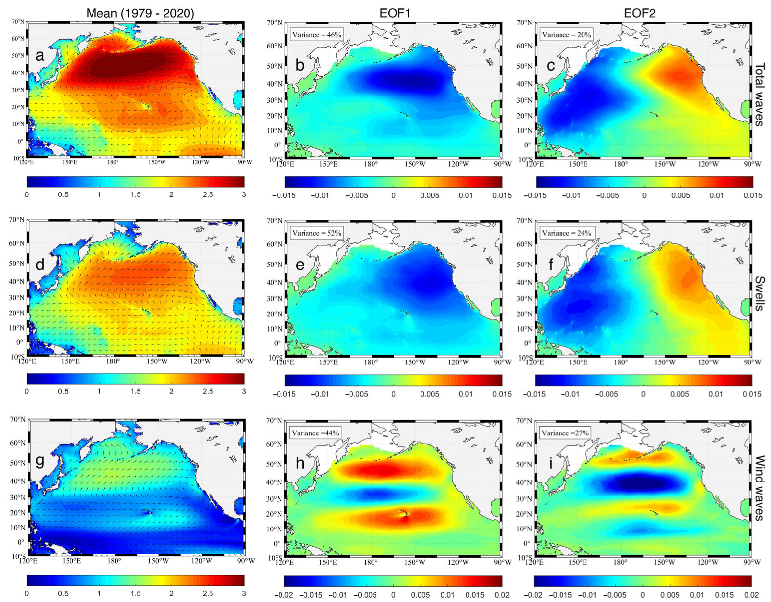
3.1. Spatial and Temporal Distribution of Wave Height

The high wave heights in the NP, influenced by low-pressure systems, concentrate in the mid-latitudes of the NP as shown in Figure 1a. In the NP, wave direction typically exhibits northeastward propagation at middle and high latitudes, while low latitudes are characterized by southwestward propagation. Nonetheless, it is worth noting that a northward-propagating component can be observed in the equatorial eastern Pacific. To explore the relationship between NP waves and large-scale climate phenomena, our study focused on analyzing the long-term variation of the SWH. Different latitudes have similar main periods, consisting of 10.5, 6.0, 4.7, and 3.0 years periods by using the FFT method as shown in Figure 2. Table 1 also shows the results. Notably, the main period of ENSO is 2–7 years. It is plausible that the cycles of 3.0, 4.7, and 6.0 years could be linked to ENSO signals. This finding suggests that the ENSO signal may be present in the NP wave field.
To further comprehend the spatial and temporal characteristics of the SWH field in the NP, we analyze the abnormal monthly total wave heights in the NP using the EOF method. Figure 1b,c presents the first two spatial modes of EOF separately. The variance contribution of the first mode of EOF (EOF1) is 46% and is dominated by negative anomalies, with the center of negative anomalies extending southeastward from the west coast of North America to the mid-latitudes of the NP. The spatial distribution of EOF2 is dominated by the east–west inverse phase distribution, with the center of positive anomalies dominating in the east Pacific and the center of negative anomalies dominating in the west Pacific. Additionally, the FFT of PC1 indicates the main periods are 6.0 years, 4.7 years, and 3.0 years, as shown in Table 2. This corresponds to the period of ENSO and that of abnormal monthly SWH. These findings further support the existence of ENSO signals within the wave field of the NP.
Previous studies have confirmed that ENSO events are accompanied with SST anomalies and SWH anomalies in the NP [28]. Therefore, we conduct a case analysis of the years with ENSO events. Figure 3 illustrates the distribution of the anomalous SWH in 1989 (La Niña year) and 1998 (El Niño year). In 1989, the Niño3 index was −0.66 and was 2.34 in 1998. These two years are chosen because 1989 is the strongest year of the La Niña event in the time frame of this paper, and 1998 is the strongest year of the El Niño event in the time frame of this paper. The spatial distribution of wave fields for El Niño and La Niña years demonstrates opposing phases, and the center of SWH anomalies is situated near the west coast of North America. During El Niño events, negative anomalies of Aleutian low pressure are observed, accompanied by an increase in the abnormality of sea surface wind speeds, resulting in enhanced wave heights [38]. Therefore, a positive anomaly of wave heights occurred in the North Pacific in 1998. During El Niño years, the equatorial eastern Pacific experiences an increase in SST anomaly, whereas the northeastern Pacific presents an increase in SWH anomaly, which is reversed during La Niña years.

3.2. Spatial and Temporal Distribution of Swells and Wind Waves

Ocean waves can be divided into swells and wind waves. To discern the significant impacts of wind waves and swells on a larger scale, it is imperative to acquire a comprehensive comprehension of their distinct spatial dispersion.
Wind waves originating in the mid-latitudes of the NP spread eastward as shown in Figure 1g. Part of swells propagates southward into the lower latitudes of the NP. North of 30° N, Pacific swells exhibit a northeastward propagation pattern, while manifesting a northwestward trend in the western NP. Conversely, the swells south of 30° N demonstrate a southwestern trajectory, with a northward component observed in low latitudes of the eastern NP, as depicted in Figure 1d. Generally, the SWH of swells in the NP is higher than the SWH of wind waves. This means that the overall energy of swells in the NP is greater than that of wind waves.
To understand the spatial distribution of swells and wind waves, we calculate the time series of abnormal monthly wind waves and swells in different latitudes, as illustrated in Figure 4. The anomalies of swells and wind waves are primarily concentrated within the range from −0.2 m to 0.2 m. Figure 4 show that the extreme anomalies correspond to the years 1989 and 1998, which are marked by typical La Niña and El Niño events, respectively. However, the wind wave height anomaly in 20° N latitude is not obvious in 1998. Comparison of the time series of wind waves and swell anomalies and the Niño3 index reveals that both show a positive correlation with the Niño3 index, especially the swell anomalies. Therefore, the swell height anomaly is more closely related to El Niño. This observation leads us to speculate that there could be a connection between swells and wind waves and El Niño, as well as between the NP wave field and El Niño. Then, we intend to undertake a case study of these special years to validate our hypothesis.
The northeastern Pacific swells are observed to possess a southward component as shown in Figure 1d. To gain a deeper understanding of its pattern of variation, we perform an EOF analysis of the swells and wind wave anomalies. Figure 1e,f,h,i illustrate the first two EOF spatial modes (EOF1 and EOF2) of wind waves and swells SWH anomalies. The variance contribution of EOF1 is 52% and 24%, respectively. The spatial distribution of EOF1 in Figure 1e shows that the anomalous signal of the swells could be transported southward in the NP. There is a negative anomaly center in the northeastern part of the NP, and previous studies have shown the existence of a swell pool here [38], so the southward propagation of the swell along the west coast of the United States can reach the equatorial region. EOF2 demonstrates an east–west inverse phase distribution. The center of the positive anomaly in the eastern NP increases from north to south in a meridional direction.
The wind waves’ EOF1 modes alternate with positive and negative anomalies from north to south as shown in Figure 1h. The same spatial distribution is observed in the wind wave field shown in Figure 1g. The distribution of wind wave EOF2 in space is the same as that of wind wave EOF1 as depicted in Figure 1i.

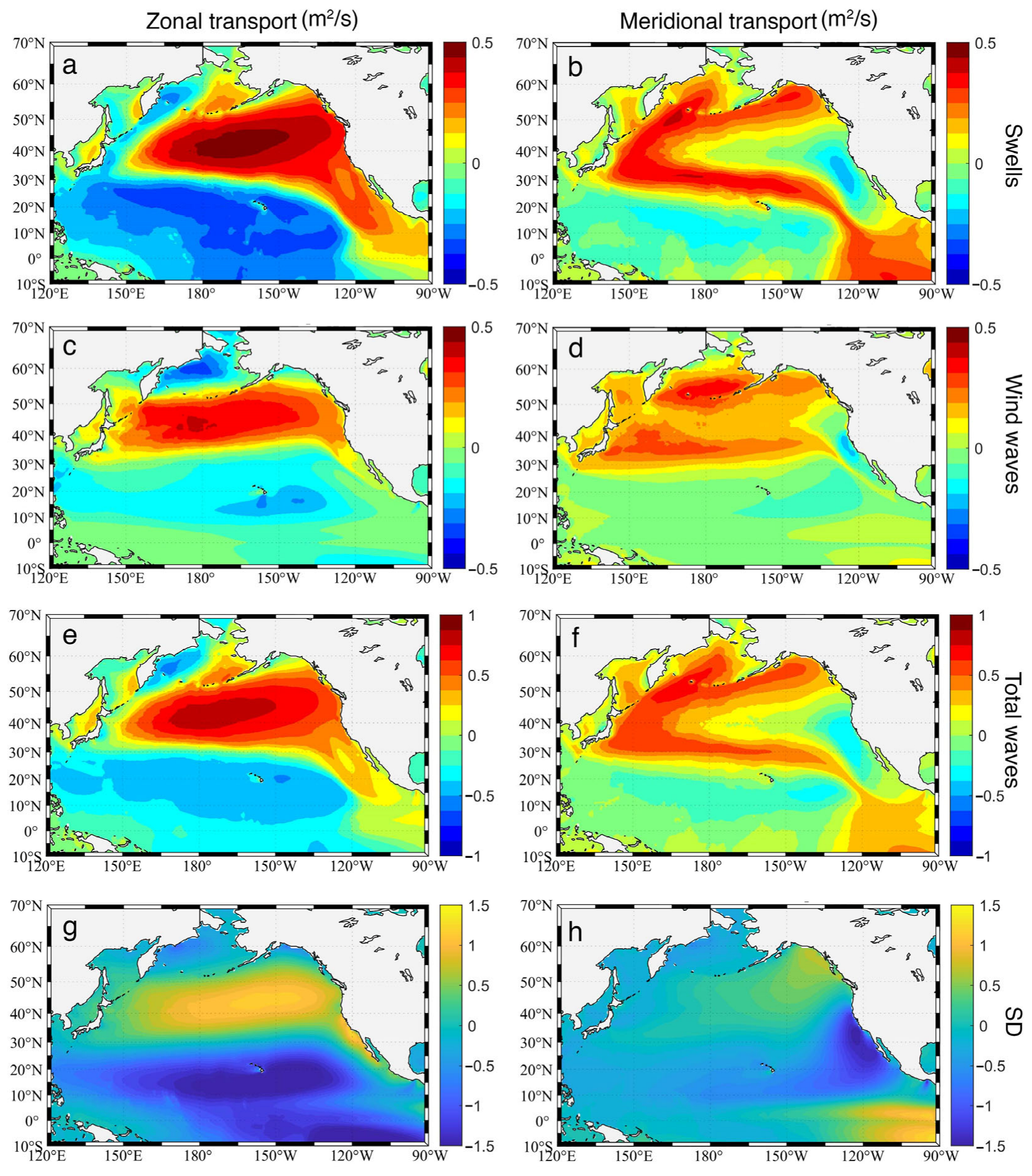
3.3. Wave-Induced Water Transport

The predominant methods of calculating wave-induced transport are currently parametric method and spectral method. In this paper, the calculation of wind wave-induced transport and swell-induced transport use the parametric method, while the spectral method uses the surface SD to calculate wave transport.
The spatial distribution of swells and wind waves, as evidenced by Figure 1d,g, reveals that their directions and height are not identical. Therefore, the wave transport induced by each also differs. With Equation (1), we calculate the meridional and zonal wave transport induced by wind waves and swells through the parametric method, as shown in Figure 5a–d. From the spatial distribution, the zonal wave transport induced by wind waves generally propagates eastward at mid-latitudes and westward at low latitudes, which is consistent with the direction of wind waves. The results indicate that the values of wave transport at mid-latitudes surpass low latitudes. The spatial distribution of the zonal wave transportation caused by swells and wind waves is roughly the same. It is worth noting that in the eastern boundary of the NP, swell-induced eastward wave transport from mid-latitudes extends to the equatorial region.
The wind wave-induced meridional wave transport propagates northward in the middle and high latitudes, and the transport values are smaller in the low latitudes, as shown in Figure 5d. Swell-induced meridional wave transport exhibits a “C”-shaped northward propagation in the north of 25° N. Swell-induced wave transport at the eastern boundary of the Pacific Ocean can be transported from the mid-latitudes of the NP to the low-latitude region. This result is consistent with that of Figure 1f. So, it would transport the cold water from higher latitudes to lower latitudes and would decrease the SST in tropical latitudes.
The total wave-induced meridional and zonal wave transport in the NP is obtained using the parameter method, as depicted in Figure 5e,f. The spatial distribution indicates that the zonal direction aligns with the wind wave-induced zonal wave transport in Figure 5c, while the meridional direction aligns with the swell-induced meridional wave transport. Based on the available data and analysis, it can be inferred that in the northern hemisphere, the zonal wind wave-induced wave transport prevails, whereas the meridional swell-induced wave transport is dominant.
The utilization of surface SD for calculating wave transport is regarded as a more precise method compared to the parametric approach [39,40]. The spatial distribution of SD-induced wave transport in the zonal and meridional surfaces of the NP, calculated by the spectral method using Equation (4), is shown in Figure 5g,h. The large values of zonal surface SD transport are located near 15° N and 45° N, with mean values greater than 1.5 m²/s. Meridionally, the overall surface SD-induced wave transport is northward north of 30° N and southward south of 30° N. Along the southern North American coast, the southward transport can extend to 40° N. This indicates that waves from higher latitudes of the NP can induce wave transport to equatorial areas.
Comparing the two methods of calculating wave transport in Figure 5e–h, the wave transport calculated by the spectral method is larger than that calculated by the parametric method. The spatial distribution of the zonal wave transport calculated by the parametric and spectral methods is basically the same, while the spatial distribution of the meridional direction has a little different. The parametric method yields large values of meridional wave transport that are mainly focused on the western NP, whereas the spectral method yields extreme values of meridional wave transport that are predominantly concentrated in the western coastline of North America.
The meridional and zonal surface SD transport anomalies are further examined through the application of the EOF method. As shown in Figure 6a,c, the positive and negative anomaly centers of EOF1 and EOF2 in the zonal SD transport alternate along the meridional direction. Conversely, the meridional SD transport anomalies alternate along the zonal direction as shown in Figure 6b,d. In the NP, the zonal SD transport anomalies are prominent in the mid-latitudes. This is similar to the distribution of wind waves anomalous EOF in Figure 1h,i. As for the EOFs with meridional SD transport, there is an anomaly center in the northeast NP, with the corresponding anomalies expanding southward. From the variance contribution shown in Figure 6, it is determined that the first two EOFs of both meridional SD transport and zonal SD transport can effectively describe their primary features, accounting for 99.9% of the total variance.

4. The Relationship between Surface Stokes Drift and ENSO

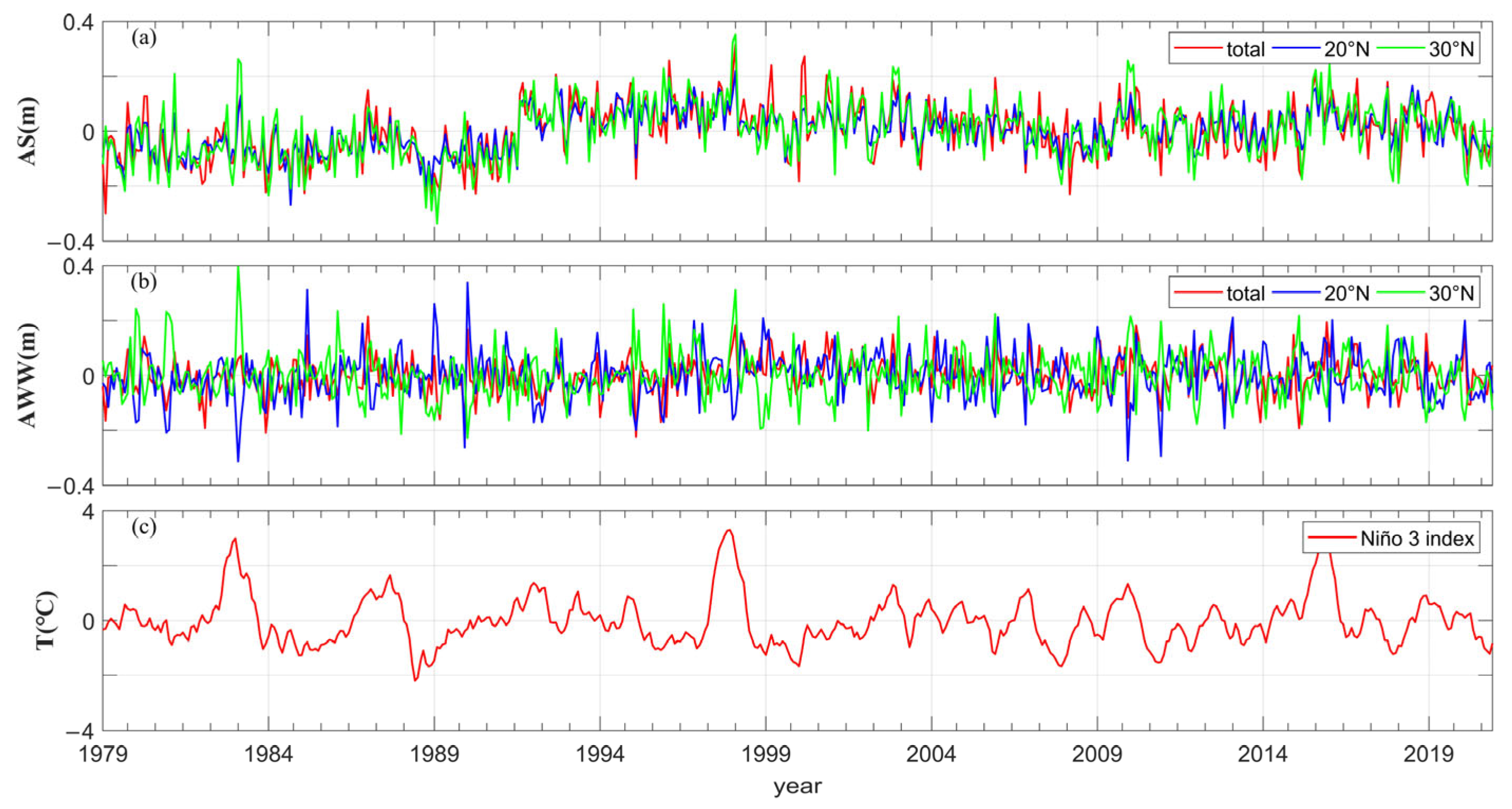
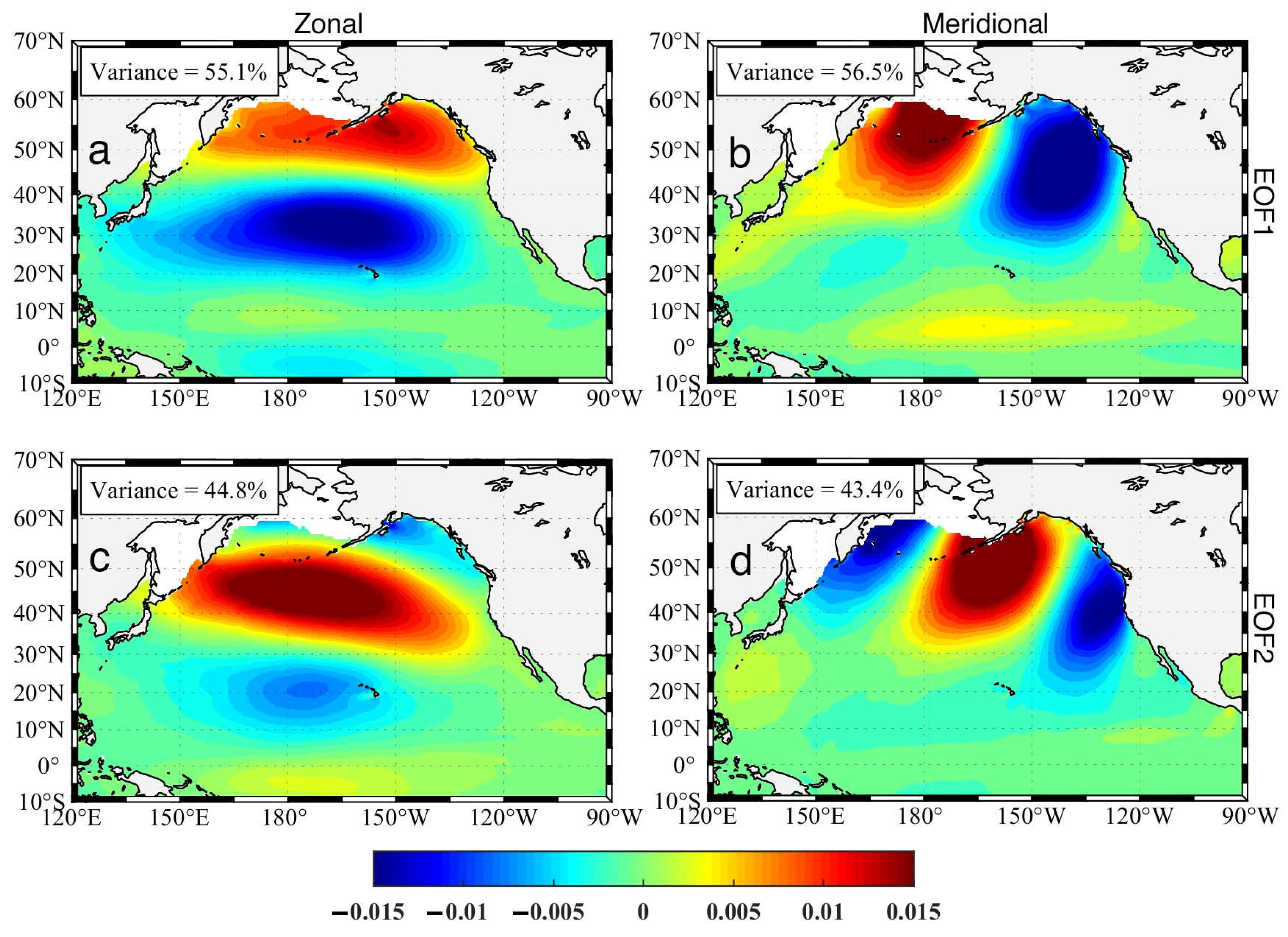
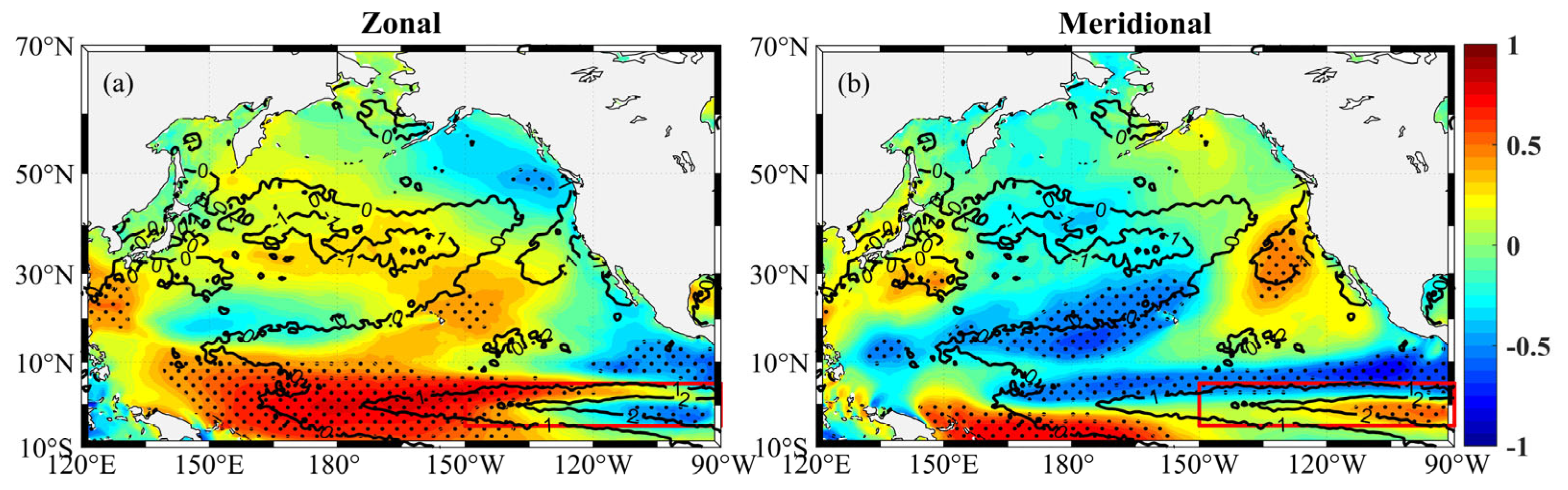
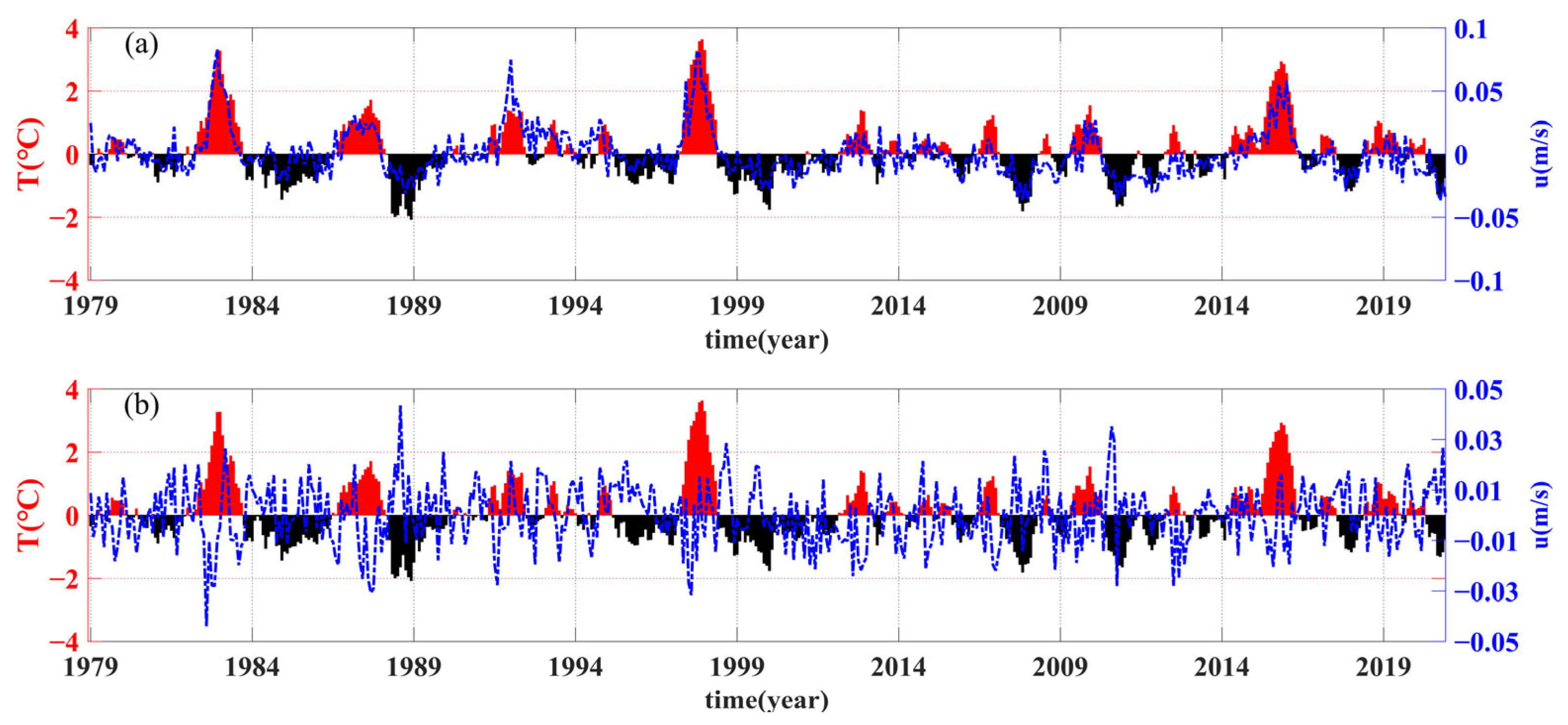
4.1. Correlation between Surface Stokes Drift and ENSO
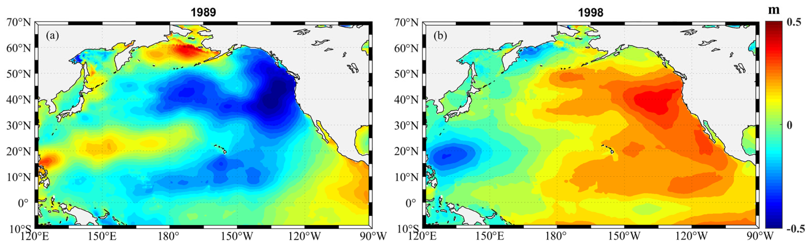
The meridional wave transport in the South Pacific exhibits a robust association with the ENSO, while the northward wave transport originating from the South Pacific contributes favorably to the attenuation of El Niño [9,41]. Therefore, we hypothesize that the NP waves also affect El Niño during the southward propagation. We conducted a direct analysis of the relationship between SD and the Niño3 index since SD is the primary factor influencing wave transport. The Niño3 SST anomaly index is an indicator of eastern tropical Pacific El Niño conditions. It is calculated with SSTs in the box 150° W–90° W, 5° S–5 °N. The Niño3 index can be obtained from: (https://climatedataguide.ucar.edu/climate-data/nino-sst-indices-nino-12-3-34-4-oni-and-tni, accessed on 1 September 2023) [42]. Figure 7 presents the spatial distribution of the correlation coefficient between the abnormal surface SD and the Niño3 index. From the spatial distribution, the correlation coefficients of the meridional and zonal directions in the Niño3 region show an overall opposite trend, with the absolute values of the correlation coefficients being over 0.6. The results obtained from the correlation coefficient distribution of the zonal and meridional SD anomalies indicate that significant correlations exist between the wave transport anomalies and SST anomalies in the eastern equatorial Pacific. During the occurrence of El Niño, the trade winds near the equator become weaker, resulting in a decrease in the westward wave. Consequently, this leads to a positive anomaly in zonal transport. Furthermore, as depicted in Figure 7b, the meridional SD propagates towards the equator at both low latitudes in the North and South Pacific.
The correlation coefficient between the eastward and northward surface SD anomalies and the Niño3 index is 0.82 and −0.72, respectively. To further understand the correlation between ENSO and the surface SD anomaly, we select the western interface of the Niño3 region (150° W, 5° S–5° N) and compare the time series of the surface SD abnormal monthly average through this interface with the Niño3 index in the past 42 years. As shown in Figure 8a, the two variables show a high positive correlation change. When El Niño events occur, the interface is often accompanied by positive surface SD anomalies. So, there is an increase in wave transport anomalies in the eastward direction through this interface. During the period of the El Niño event, the anomalous increase in temperature was concentrated in the east–central equatorial Pacific, and the temperature change in the western equatorial Pacific was not significant. As a result, there is no anomalous change in temperature in the western Pacific, even though it is a warm pool. Thus, wave-induced transport from the western Pacific to the eastern Pacific is colder water compared with the abnormal temperature in the eastern Pacific. The SD moves eastward in the equatorial west Pacific, leading to the transportation of abnormal cold water from the equatorial western Pacific. Consequently, this movement results in a reduction of SST in the equatorial eastern Pacific, which contributes positively to the restoration of the normal SST of the equatorial eastern Pacific. The zonal wave transport may play a moderating role in the SST anomaly in the equatorial eastern Pacific. Similarly, the opposite process occurs in a La Niña year, where wave transport typically moves westward.
Then, we select the northern interface of the Niño3 region (150° W–90° W, 5° N) and compare the surface SD abnormal monthly average through this interface with the Niño3 index over the past 42 years, as shown in Figure 8b. The surface SD anomalies and the Niño3 index show a negative correlation. When El Niño years occur, the SST is abnormally high in the equatorial eastern Pacific, which causes more waves to propagate southward in the North Pacific. Then, SD transports more cold water to propagate to the equatorial region to restore the SST to normal, so the interface is often accompanied by the appearance of negative surface SD anomalies. A positive SST anomaly in the equatorial eastern Pacific results in increased southward propagation of cold water by the SD from the middle and high latitudes of the NP. This, in turn, leads to a stronger suppression of SST warming in the equatorial eastern Pacific region. Therefore, the meridional wave transport also plays a moderating role on the SST anomaly in the equatorial eastern Pacific. Similarly, during La Niña years, it usually results in a reduction of the southward cold wave transport.

4.2. Case Study

As mentioned above, the correlation between the ENSO events and the SD anomalies is evident. So, we choose two typical ENSO event years (La Niña event in 1989 and El Niño event in 1998) and the average of all ENSO events (El Niño events and La Niña events) over the study time frame and show the distribution of anomalous SD in the zonal and meridional directions in Figure 9, respectively. The spatial distribution corresponding to the La Niña events and the El Niño events shows an inverse phase distribution pattern. During an El Niño occurrence, there is a significant increase in SST within the equatorial eastern Pacific Ocean. Propagation of water transport southward along the eastern boundary of the NP occurs from the mid-latitudes and brings cold water to the equatorial region. This process would have a cooling effect on El Niño. In La Niña years, the zonal transport is westward in the mid-latitudes and eastward in the low latitudes of the NP; in El Niño years, the transport is eastward in the mid-latitudes and westward in the low latitudes. To regulate SST anomaly, waves facilitate the transportation of cold water from the equatorial western Pacific Ocean towards the east, resulting in a faster restoration of the SST to its normal temperature.

5. Discussion

In previous research [9], we discovered the presence of the ACW signal in the south Pacific Ocean wave field, which occurs within a 5-year period. This signal originates in the Southern Ocean and propagates to the lower equatorial latitudes through northward swell. Following El Niño events, there is an abnormal increase in northward wave transport in the South Pacific region. Wave transport also plays a positive role in maintaining the stability of low-latitude SST in the South Pacific by transporting more or less cold water to the tropical oceans. This paper, in combination with our previous results, highlights the occurrence of El Niño events with wave-induced cold water movement from the North Pacific towards the equator. The main focus of this paper is on the effects of meridional wave transport. In our study of the relationship between IOD and wave transport in the Indian Ocean [43], we concentrate on zonal transport. Zonal wave transport can also significantly impact the IOD. Furthermore, in the Pacific Ocean, zonal wave transport may influence different types of El Niño, such as the central and eastern types. This will be the focus of our future research plan.

6. Summary

Using the 42 years of ECMWF ERA5 reanalysis data, we find that signals of the same period as ENSO exist in the wave field in the NP. By analyzing the spatial distribution of waves in the NP, our findings indicate that waves could transport wave signals from the mid- and high-latitude regions to the low-latitude regions. This paper also investigates the relationship between SD transport and the Niño3 index. The results reveal a significant correlation between the Niño3 index and SD in the low latitudes, with absolute values of correlation coefficients >0.6. Zonally, in El Niño years (La Niña years), SD may play a significant role in transportation of water towards the western (eastern) Pacific, contributing to the regulation of SST in the equatorial region. Meridionally, in El Niño years (La Niña years), SD transports more (less) cold water southward from the mid-latitudes of the NP to regulate SST in the equatorial region.
The interaction between atmosphere and ocean is influenced by waves, which hold a significant place in affecting climate at a large scale. During the El Niño (La Niña) periods, waves can contribute positively to the preservation of sea surface temperature (SST) stability in low latitudes by facilitating the transport of increased (decreased) quantities of cold water to the tropical ocean. This phenomenon can be regarded as an essential component of the self-regulating nature of the ocean–atmosphere system. This paper undertakes a discussion and analysis of specific years, with the understanding that this exploration is preliminary in nature. Furthermore, it is important to acknowledge that the global climate represents a complex and multifaceted system, where waves constitute only a fraction of the larger framework. Describing the physical mechanisms of global climate solely based on the influence of waves is insufficient and segmentary. It is necessary to conduct detailed research from multiple perspectives to better refine and explain it. Moreover, considering the potential impacts of climate change, it is expected that both ocean waves [43] and the ENSO will undergo changes [44,45]. Understanding how their relationship will evolve in response to these changes presents an intriguing area for future research.

Author Contributions

Conceptualization, X.Z. and R.L.; formal analysis, K.W.; funding acquisition, K.W.; investigation, S.Z.; methodology, S.Z.; project administration, R.L.; resources, K.W.; validation, K.W. and X.Z.; Visualization, R.L. and J.L.; writing—original draft, X.Z. and R.Z.; writing—review and editing, A.V.B., X.Z. and R.L. All authors have read and agreed to the published version of the manuscript.

Funding

This research was funded by the National Natural Science Foundation of China under grant numbers 42176018.

Data Availability Statement

The data used in this study are all provided by European Centre for Medium-Range Weather Forecasts (ECMWF) (https://cds.climate.copernicus.eu/cdsapp#!/dataset/reanalysisera5-single-levels monthly-means?tab=form, accessed on 1 September 2023).

Acknowledgments

The authors thank the researchers who obtained and published the data and schemes used in this study. R.L. acknowledges the fellowship provided by the China Scholarship Council (CSC:202206330001).

Conflicts of Interest

The authors declare that the research was conducted in the absence of any commercial or financial relationships that could be construed as a potential conflict of interest.

References

  1. Mcwilliams, J.C.; Restrepo, J.M. The wave-driven ocean circulation. J. Phys. Oceanogr. 1999, 29, 2523–2540. [Google Scholar] [CrossRef]
  2. Wu, K.; Liu, B. Stokes drift–induced and direct wind energy inputs into the Ekman layer within the Antarctic Circumpolar Current. J. Geophys. Res. Oceans 2008, 113. [Google Scholar] [CrossRef]
  3. Liu, B.; Wu, K.; Guan, C. Global estimates of wind energy input to subinertial motions in the Ekman-Stokes layer. J. Oceanogr. 2007, 63, 457–466. [Google Scholar] [CrossRef]
  4. Polton, J.A.; Lewis, D.M.; Belcher, S.E. The role of wave-induced Coriolis-Stokes forcing on the wind-driven mixed layer. J. Phys. Oceanogr. 2005, 35, 444–457. [Google Scholar] [CrossRef]
  5. Hill, R.H. Laboratory measurement of heat transfer and thermal structure near an Air-Water interface. J. Phys. Oceanogr. 1972, 2, 190–198. [Google Scholar] [CrossRef]
  6. Tamura, H.; Miyazawa, Y.; Oey, L.Y. The Stokes drift and wave induced-mass flux in the North Pacific. J. Geophys. Res. Oceans 2012, 117. [Google Scholar] [CrossRef]
  7. Janssen, P.A.E.M.; Breivik, Ø.; Mogensen, K.; Vitart, F.; Balmaseda, M.; Bidlot, J.-R.; Keeley, S.; Leutbecher, M.; Magnusson, L.; Molteni, F. Air-Sea Interaction and Surface Waves; European Centre for Medium-Range Weather Forecasts: Reading, UK, 2013. [Google Scholar]
  8. Zheng, C.; Wu, D.; Wu, H.; Guo, J.; Shen, C.; Tian, C.; Tian, X.; Xiao, Z.; Zhou, W.; Li, C. Propagation and attenuation of swell energy in the Pacific Ocean. Renew. Energ. 2022, 188, 750–764. [Google Scholar] [CrossRef]
  9. Li, R.; Wu, K.; Li, J.; Akhter, S.; Dong, X.; Sun, J.; Cao, T. Large-scale signals in the south pacific wave fields related to ENSO. J. Geophys. Res. Oceans 2021, 126, e2021JC017643. [Google Scholar] [CrossRef]
  10. Bromirski, P.D.; Flick, R.E.; Graham, N. Ocean wave height determined from inland seismometer data; Implications for investigating wave climate changes in the NE Pacific. J. Geophys. Res. Oceans 1999, 104, 20753–20766. [Google Scholar] [CrossRef]
  11. Allan, J.; Komar, P. Are ocean wave heights increasing in the eastern North Pacific? Eos Trans. Amer. Geophys. Union. 2000, 81, 561. [Google Scholar] [CrossRef]
  12. Ruggiero, P.; Komar, P.D.; Allan, J.C. Increasing wave heights and extreme value projections: The wave climate of the U.S. Pacific Northwest. Coast. Eng. 2010, 57, 539–552. [Google Scholar] [CrossRef]
  13. Hemer, M.A.; Church, J.A.; Hunter, J.R. Variability and trends in the directional wave climate of the Southern Hemisphere. Int. J. Climatol. 2010, 30, 475–491. [Google Scholar] [CrossRef]
  14. Sasaki, W. Changes in the North Pacific wave climate since the mid-1990s. Geophys. Res. Lett. 2014, 41, 7854–7860. [Google Scholar] [CrossRef]
  15. Gulev, S.K.; Grigorieva, V. Last century changes in ocean wind wave height from global visual wave data. Geophys. Res. Lett. 2004, 31. [Google Scholar] [CrossRef]
  16. Kako, S.; Kubota, M. Relationship between an El niño event and the interannual variability of significant wave heights in the north pacific. Atmos. Ocean 2006, 44, 377–395. [Google Scholar] [CrossRef]
  17. Hasselmann, K. On the mass and momentum transfer between short gravity waves and larger-scale motions. J. Fluid Mech. 1971, 50, 189–205. [Google Scholar] [CrossRef]
  18. Shi, Y.; Wu, K.; Zhu, X.; Yang, F.; Zhang, Y. Study of relationship between wave transport and sea surface temperature anomaly (SSTA)in the tropical Pacific. Acta Oceanol. Sin. 2016, 35, 58–66. [Google Scholar] [CrossRef]
  19. Lukas, R.; Yamagata, T.; Mccreary, J.P. Pacific low-latitude western boundary currents and the Indonesian throughflow. J. Geophys. Res. Oceans 1996, 101, 11867–12488. [Google Scholar] [CrossRef]
  20. Wu, L.; Cai, W.; Zhang, L.; Nakamura, H.; Timmermann, A.; Joyce, T.; Mcphaden, M.J.; Alexander, M.; Qiu, B.; Visbeck, M.; et al. Enhanced warming over the global subtropical western boundary currents. Nat. Clim. Chang. 2012, 2, 161–166. [Google Scholar] [CrossRef]
  21. Sun, X.; Wu, R. Spatial scale dependence of the relationship between turbulent surface heat flux and SST. Clim. Dynam. 2022, 58, 1127–1145. [Google Scholar] [CrossRef]
  22. Carrasco, A.; Semedo, A.; Isachsen, P.E.; Christensen, K.H.; Saetra, Ø. Global surface wave drift climate from ERA-40: The contributions from wind-sea and swell. Ocean Dynam. 2014, 64, 1815–1829. [Google Scholar] [CrossRef]
  23. Li, X.; Hu, Z.; Huang, B. Contributions of Atmosphere–Ocean Interaction and Low-Frequency Variation to Intensity of Strong El Niño Events since 1979. J. Clim. 2019, 32, 1381–1394. [Google Scholar] [CrossRef]
  24. Kang, I.; An, S. Kelvin and rossby wave contributions to the SST oscillation of ENSO. J. Clim. 1998, 11, 2461–2469. [Google Scholar] [CrossRef]
  25. Kim, K.Y.; Kim, Y.Y. Mechanism of Kelvin and Rossby waves during ENSO events. Meteorol. Atmos. Phys. 2002, 81, 169–189. [Google Scholar] [CrossRef]
  26. Park, J.; Sung, M.; Yang, Y.; Zhao, J.; An, S.; Kug, J. Role of the climatological intertropical convergence zone in the seasonal footprinting mechanism of the El Niño-Southern Oscillation. J. Clim. 2021, 5243–5256. [Google Scholar] [CrossRef]
  27. Aramburo, D.; Montoya, R.D.; Osorio, A.F. Impact of the ENSO phenomenon on wave variability in the Pacific Ocean for wind sea and swell waves. Dynam. Atmos. Oceans 2022, 100, 101328. [Google Scholar] [CrossRef]
  28. Izaguirre, C.; Méndez, F.J.; Menéndez, M.; Losada, I.J. Global extreme wave height variability based on satellite data. Geophys. Res. Lett. 2011, 38. [Google Scholar] [CrossRef]
  29. Dee, D.P.; Uppala, S.M.; Simmons, A.J.; Berrisford, P.; Poli, P.; Kobayashi, S.; Andrae, U.; Balmaseda, M.A.; Balsamo, G.; Bauer, P.; et al. The ERA-Interim reanalysis: Configuration and performance of the data assimilation system. Q. J. Roy. Meteor. Soc. 2011, 137, 553–597. [Google Scholar] [CrossRef]
  30. Hersbach, H.; Bell, B.; Berrisford, P.; Hirahara, S.; Horányi, A.; Muñoz Sabater, J.; Nicolas, J.; Peubey, C.; Radu, R.; Schepers, D.; et al. The ERA5 global reanalysis. Q. J. Roy. Meteor. Soc. 2020, 146, 1999–2049. [Google Scholar] [CrossRef]
  31. Semedo, A.K.S.A. Variability of Wind Sea and Swell Waves in the North Atlantic Based on ERA-40 Re-analysis. In Proceedings of the 8th European Wave and Tidal Energy, Uppsala, Sweden, 7–10 September 2009; pp. 119–129. [Google Scholar]
  32. Breivik, Ø.; Janssen, P.A.E.M.; Bidlot, J. Approximate stokes drift profiles in deep water. J. Phys. Oceanogr. 2014, 44, 2433–2445. [Google Scholar] [CrossRef]
  33. Brenner, N.; Rader, C. A New Principle for Fast Fourier Transformation. IEEE Acoust. Speech Signal Process. 1976, 24, 264–266. [Google Scholar]
  34. Lorenz, E.N. Empirical Orthogonal Functions, and Statistical Weather Prediction; Massachusetts Institute of Technology, Department of Meteorology: Cambridge, MA, USA, 1956. [Google Scholar]
  35. Liu, J.; Wang, Y.; Yuan, Y.; Xu, D. The response of surface chlorophyll to mesoscale eddies generated in the eastern South China Sea. J. Oceanogr. 2020, 76, 211–226. [Google Scholar] [CrossRef]
  36. Wang, Y.; Liu, J.; Liu, H.; Lin, P.; Yuan, Y.; Chai, F. Seasonal and interannual variability in the sea surface temperature front in the eastern Pacific Ocean. J. Geophys. Res. Oceans 2021, 126, e2020JC016356. [Google Scholar] [CrossRef]
  37. Sreelakshmi, S.; Bhaskaran, P.K. Regional wise characteristic study of significant wave height for the Indian Ocean. Clim. Dynam. 2020, 54, 3405–3423. [Google Scholar] [CrossRef]
  38. Liu, J.; Meucci, A.; Young, I.R. A comparison of multiple approaches to study the modulation of ocean waves due to climate variability. J. Geophys. Res. Oceans 2023, 1489, e2023JC019843. [Google Scholar] [CrossRef]
  39. Alves, J.G.M. Numerical modeling of ocean swell contributions to the global wind-wave climate. Ocean Model. 2006, 11, 98–122. [Google Scholar] [CrossRef]
  40. Cavaleri, L.; Fox-Kemper, B.; Hemer, M. Wind waves in the coupled climate system. B. Am. Meteorol. Soc. 2012, 93, 1651–1661. [Google Scholar] [CrossRef]
  41. Babanin, A.V.; Onorato, M.; Qiao, F. Surface waves and wave-coupled effects in lower atmosphere and upper ocean. J. Geophys. Res. Oceans 2012, 117. [Google Scholar] [CrossRef]
  42. Trenberth, K.; National Center for Atmospheric Research Staff. The Climate Data Guide: Nino SST Indices (Nino 1+2, 3, 3.4, 4; ONI and TNI). Available online: https://climatedataguide.ucar.edu/climate-data/nino-sst-indices-nino-12-3-34-4-oni-and-tni (accessed on 25 July 2023).
  43. Li, R.; Wu, K.; Li, J.; Dong, X.; Sun, J.; Zhang, W.; Liu, Q. Relating a large-scale variation of waves in the indian ocean to the IOD. J. Geophys. Res. Oceans 2022, 127. [Google Scholar] [CrossRef]
  44. Liu, J.; Meucci, A.; Young, I.R. Projected wave climate of Bass Strait and south-east Australia by the end of the twenty-first century. Clim. Dyn. 2022, 60, 393–407. [Google Scholar] [CrossRef]
  45. Liu, J.; Meucci, A.; Young, I.R. Projected 21st century wind-wave climate of Bass Strait and south-east Australia: Comparison of EC-Earth3 and ACCESS-CM2 climate model forcing. J. Geophys. Res. Oceans 2023, 128, e2022JC018996. [Google Scholar] [CrossRef]
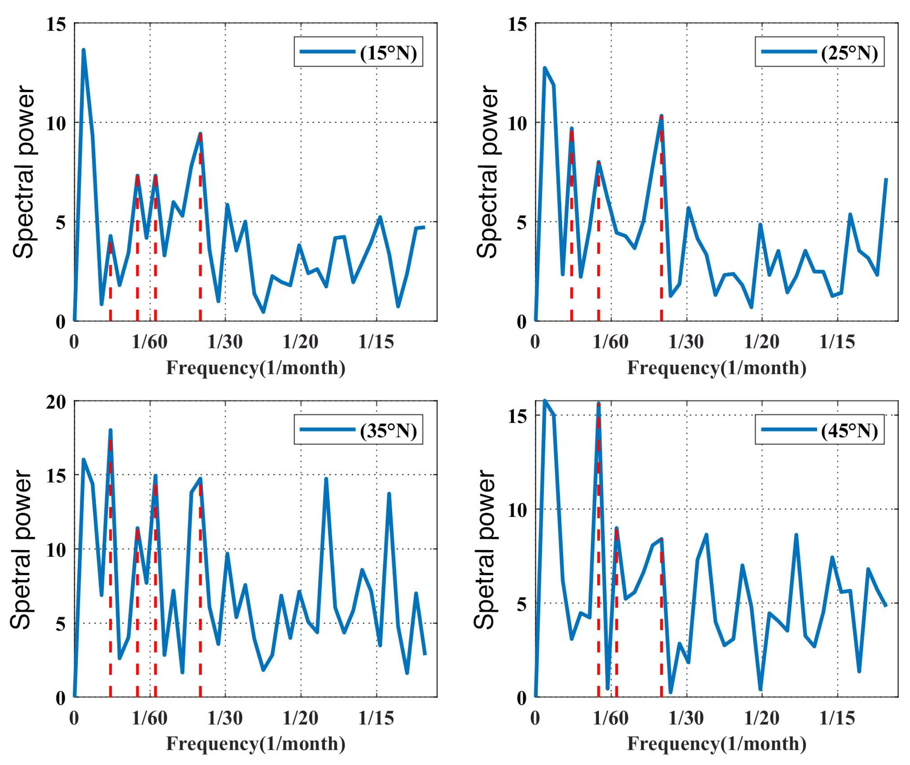
Figure 1. (a) Mean significant wave height (SWH) and directions of total waves over the period 1979–2020. (b) EOF1 of abnormal SWH of total waves. (c) EOF2 of abnormal SWH of total waves. (d) Mean significant wave height (SWH) and directions of swells over the period 1979–2020. (e) EOF1 of abnormal SWH of swells. (f) EOF2 of abnormal SWH of swells. (g) Mean significant wave height (SWH) and directions of wind waves over the period 1979–2020. (h) EOF1 of abnormal SWH of wind waves. (i) EOF2 of abnormal SWH of wind waves. The explained variances of EOFs are indicated in each panel.
Jmse 11 01848 g001
Figure 2. FFT analysis of monthly SWH anomalies along the 15° N, 25° N, 35° N and 45° N latitudes from 150° E to 135° W.
Jmse 11 01848 g002
Figure 3. SWH abnormal monthly average of total waves in 1989 (a) and 1998 (b).
Jmse 11 01848 g003
Figure 4. Monthly values of SWH anomalies of swells (a) and wind waves (b) in the entire NP, 20° N and 30° N and the Niño3 index (c) from 1979–2020. Where AS means abnormal swells, AWW means abnormal wind waves.
Jmse 11 01848 g004
Figure 5. Zonal and meridional wave transports (m2/s) induced by swells (a,b), wind waves (c,d), total waves (e,f) and SD (g,h). (af) are based on parameter method, while (g,h) are based on spectral method. Northward and eastward transports are defined as positive.
Jmse 11 01848 g005
Figure 6. EOF1 (a,b) and EOF2 (c,d) of zonal (a,c) and meridional (b,d) SD transport anomalies.
Jmse 11 01848 g006
Figure 7. Correlation coefficients between zonal (a)/meridional (b) SD anomalies (detrended seasonal averages) and the Niño3 index. The red boxes represent the Niño3 region. The black lines indicate the SST anomaly contours. The black dots indicate the >99% confidence level.
Jmse 11 01848 g007
Figure 8. Time series of eastward (a) and northward (b) surface SD abnormal monthly average (blue lines) across the western interface (150° W, 5° S–5° N) and the northern interface (150° W–90° W, 5° N)and the Niño3 index (bars) over the period 1979–2020. The red (black) bars represent El Niño (La Niña) years.
Jmse 11 01848 g008
Figure 9. Zonal and meridional surface SD abnormal monthly average (m/s) in 1989 (a,b), 1998 (c,d), average of La Niña years (e,f) and average of El Niño year (g,h). Northward and eastward are defined as positive.
Jmse 11 01848 g009
Table 1. The main period of the abnormal monthly average of SWH from 1979 to 2020.
LatitudeFrequency (1/Month)Period/(Month)Period/(Year)
15° N0.028363.0
0.014726.0
0.018564.7
0.00812610.5
25° N0.028363.0
0.00812610.5
0.014726.0
35° N0.00812610.5
0.028363.0
0.018564.7
0.014726.0
45° N0.00812610.5
0.014726.0
0.028363.0
Table 2. Main periods of the abnormal total wave heights PC time series for 1979–2020.
PCFrequency (1/Month)Period/(Year)
PC10.0146.0
0.0283.0
0.0184.7
PC20.00810.5
0.0561.5
0.024.2
Disclaimer/Publisher’s Note: The statements, opinions and data contained in all publications are solely those of the individual author(s) and contributor(s) and not of MDPI and/or the editor(s). MDPI and/or the editor(s) disclaim responsibility for any injury to people or property resulting from any ideas, methods, instructions or products referred to in the content.

