Article

Fast Reconstruction Model of the Ship Hull NURBS Surface with Uniform Continuity for Calculating the Hydrostatic Elements

1
Navigation College, Dalian Maritime University, Dalian 116026, China
2
Key Laboratory of Navigation Safety Guarantee of Liaoning Province, Dalian 116026, China
*
Author to whom correspondence should be addressed.
J. Mar. Sci. Eng. 2023, 11(9), 1816; https://doi.org/10.3390/jmse11091816
Submission received: 28 August 2023 / Revised: 9 September 2023 / Accepted: 14 September 2023 / Published: 18 September 2023
(This article belongs to the Topic Ship Dynamics, Stability and Safety)

Abstract

:
The fast reconstruction of the ship hull nonuniform rational B-spline (NURBS) surface with uniform continuity is essential for calculating hydrostatic elements such as waterplane area and molded volume in real time. Thus, this study proposes a fast reconstruction model with uniform continuity to solve the problem of uniform continuity and splicing in the separate model of hull bow and stern surfaces. The proposed model includes the NURBS curve generation (UCG) algorithm with uniform continuity and the hybrid NURBS surface generation (HSG) algorithm. The UCG algorithm initially fits the feature points using the global interpolation algorithm and then precisely constructs straight-line segments in the curve using the improved flattening algorithm. In comparison, the HSG algorithm adaptively selects the surface knot vectors according to the parameters of the section curves. In this study, the profile of discontinuous compartments is uniformly expressed, effectively avoiding various articulation problems in separation modeling. The results of comparative experiments show that the NURBS surface generated using the HSG algorithm can accurately express the characteristics of various parts of the hull with uniform continuity, and the calculation speed of the proposed model can be increased by up to 8.314% compared with the existing best-performing algorithms. Thus, the proposed model is effective and can improve computational efficiency to a certain extent. The NURBS surfaces generated by the proposed model can be further applied to calculating the hydrostatic elements of hulls and compartments.

1. Introduction

The Japan Transport Safety Board [1] (Figure 1) and the European Maritime Safety Agency [2] have reported that ship collision, contact, and grounding are the leading causes of global maritime accidents, accounting for more than 60% of ship casualties. In case of an accident, the damaged ship’s decision making with respect to the time needed to save the ship, the amount of abandoned cargo, and whether to abandon the ship depends on its real-time calculation of hydrostatic elements of damaged hull or compartments. A surface model of the hull and compartments effectively determines the hydrostatic elements of a damaged ship for calculating flotation and stability during an accident [3]. At present, the nonuniform rational B-spline (NURBS) surface is commonly used to describe the hull surface because it can accurately represent quadratic regular and freeform curved surfaces. Furthermore, the NURBS surface model can also be used to generate finite element models to analyze the performance of entities [4,5].
Generally, NURBS surfaces can be determined using the following methods: the global and local surface interpolation method [6,7], the surface approximation method [8,9], and the skinning method [10]. Additionally, particular surfaces, such as swung surfaces [11], swept surfaces [12], Gordon surface [13], and Coons surface [14], have their own generative methods. In this study, hull surfaces are used for stability analysis, which requires high-precision numerical calculations of elements such as drainage volume and waterline surface area. Hence, the surface approximation method is unsuitable in such cases. Moreover, swung surfaces and related methods are not used because hull surfaces are not considered as particular surfaces.
The global interpolation method is generally used for NURBS curve interpolation that can form rectangular meshes. He [15] used the NURBS global interpolation method to obtain freeform surfaces to establish the relationship between parameters (u, v) and independent variables (x, y, z). Bhattarai et al. [16] used the global interpolation method to generate rectangular grids. They extracted the feature grids conforming to NURBS surfaces and used the control points of these grids as interpolation points to generate NURBS surfaces. Note that a rectangular control point mesh is difficult to obtain from the interpolated point data in the application even though the global and local interpolation methods can generate surfaces faster. Hence, discarding some of the interpolated points to construct the control point mesh will reduce the accuracy of the generated surfaces.
The skinning algorithm is considered for NURBS surface interpolation where a rectangular mesh cannot be formed. The algorithm constructs a smooth and fair surface based on the section curves and resolves the issue of a nonuniform number of section curve points in the interpolated mesh. However, when applied to the hull surface representation, the algorithm generates at least several hundred interpolation points and at least thousands of control points after unifying section curve operations, such as knot refinement and degree elevation, which severely reduces the computational speed.
To address this problem, some scholars have focused on constructing surfaces with simplified knots. Park and Kim [17] proposed the use of approximation curves to represent two-dimensional section curves and reduce common knots. Piegl and Tiller [10] considered only the approximation section curves or both the approximation section curves and skinning surface point methods to obtain the sample surfaces. The advantage of both these approaches is the autonomous selection of the approximation process. Park et al. [9] modified the knot parameters of the section curves using the energy minimization method to obtain the number of knots of the approximated curve. This approach can improve the surface smoothing quality and increase the computation time while sacrificing the fitting accuracy. Park [18] proposed setting the step size by fitting the local geometry of the object surface and combining the multiple curve fitting method to transform the surface approximation into a series of curve fitting problems. This method generates fewer control points for the surface. Nevertheless, representation of the local geometry of the object is more challenging, owing to which setting reasonable adaptive sampling parameters is difficult. Moreover, it is difficult to control the accuracy of different section curve fittings uniformly within reasonable accuracy. Piegl and Tiller [19] proposed a variable knot interpolation method, instead of section curves, that exhibited higher accuracy and compatibility but required more control points and longer computation time. Overall, these methods construct a uniform knot vector by modifying the knot parameters of the section curve, alleviating the problem of insufficient compatibility of parametric or input section curves. Still, the effect of improvement is usually proportional to the error of approximation, and a relatively large accuracy needs to be sacrificed to obtain good improvement. Some researchers have focused on parameterization. Piegl and Tiller [20] proposed the selection of knot values from a predefined knot vector when interpolating section curves. Their proposed method substantially reduced the number of knots in a uniform knot vector; however, it is still a challenge to determine a better-predefined knot vector. Park [21] used a linear constraint energy minimization method to construct compatible knot vectors for generating surfaces; their proposed method effectively reduced the number of control points. However, selecting a common knot vector that contains enough degrees of freedom in a multiple interpolation point task is more challenging to guarantee the interpolation of all section curves to a given appropriate point. Shamsuddin and Ahmed [22,23] proposed a new NURBS parameterization method that effectively reduced the number of control points and generated smooth and fair hull NURBS surfaces. Nevertheless, their proposed method still lacks sufficient computational speedup with respect to multiple interpolation points and section curves.
In recent years, many scholars have successfully combined skinning algorithms with specific fields based on the above research. Wu [24] proposed an adaptive skinning algorithm that simplifies the deformation process of surfaces according to the mesh characteristics and improves the computational efficiency and rendering speed. Bang and Lee [25] updated skinning weights on the mesh through smooth interpolation and propagation of weights and realized the real-time generation of a new skinning model by changing feature points. However, their proposed method consumed too much computing time. Yin and Mukundan [26] constructed the “deform factor” parameter to determine the degree of model changes in the skinning process and effectively removed the artifacts. Although the algorithm generates models with high accuracy, its calculation speed still needs to be enhanced further. Liu et al. [27] proposed the sparse and localized skinning decomposition method to obtain the optimal parameters of the skinning model, including weights. Their proposed rigidity estimation algorithm determined the nonlinear relationship between the parameters and the deformation of the skinning model. Moutafidou et al. [28] used the skinning model and a new animated mesh sequence to construct a discriminator and a generator, respectively, to obtain a simplified model while reducing the error of model simplification. Kruppa et al. [29] proposed an intersection-free skinning method to approximate disk B-spline shapes, which effectively solved the problems of self-intersections and cusps in modeling. Thus, the skinning algorithm can obtain good results; however, the problem of computation speed has rarely been studied.
In summary, the greatest challenge in generating hull NURBS surfaces for adaptive ship calculations is finding a balance between the number of control points and the accuracy of the hull expression during the skinning process. Therefore, it is essential to determine this balance without damaging the original interpolation points.
The fast construction of the NURBS surfaces of ship hull and compartments with uniform continuity using skinning algorithms depends on the combination of section curves with the same properties. It includes setting up appropriate control point parameterization methods and calculating knot vectors, among other processes. The NURBS section curves can be generated using (1) global and local interpolation methods [19,20] and (2) global and local approximation methods [30].
Traditionally, the segmental interpolation method, i.e., a local interpolation method, is used to construct ship hull surfaces. This method uses only the local data at each step to create the curve segmentally. In comparison to other algorithms, this method can better handle cusps, straight-line segments, and some other irregular data. However, it generates relatively more internal duplicate knots, making it difficult to build the expected continuity at the joints of each segment. Thus, the resulting surface lacks uniform continuity.
The accuracy of curve point fitting and the representation of the interpolated points can be improved by considering least-square fitting [31,32], quadratic programming [33], and evolutionary algorithms [34] to change the weight vector parameters and optimize the curve. Ma and Kruth [31] used the least-square approximation for the fitting process of interpolation points and projected the three-dimensional (3D) data to the base plane for the calculation of the NURBS curve parameters. Voisin et al. [35] proposed a 3D object reconstruction method based on a genetic algorithm and point cloud data, which uses an adaptation function with a tolerance threshold to deal with errors. Cai et al. [36] proposed a NURBS- and snake-based energy minimization approach to fit NURBS curves using inverse optimization rules. However, their proposed approach assumes that all parameters, such as knots and weight vectors in the optimization framework, have fixed values from the beginning to the end, except for control points, which reduce the number of parameters in curve optimization and improve the optimization speed. Note that the optimization does not converge in complex curves. Inspired by Cai et al. [36], Saini et al. [37] proposed a two-view reconstruction method for 3D objects based on the NURBS–snake model and used the Levenberg–Marquardt method for the optimization process. They later proposed a two-step method that uses quadratic programming to obtain the optimal values of control points and weights; however, this method is not applicable to partially occluded data [33]. Lu et al. [38] used an orthogonal perspective to model the same task in NURBS–snake energy minimization. Note that the methods proposed by Saini et al. [37] and Lu et al. [38] failed to solve the problem of Cai et al. [36]. Alazzam and Alomar [39] proposed an average uniform algorithm curve optimization method, which generates random optimal solutions using a uniform distribution and then averages the optimal solutions to obtain the optimal value of the objective function. Singh and Deep [40] proposed a nonlinear optimization model for 3D-curved surfaces using the gravity search algorithm, which sets the objective function as the error function between a given measured point and a point on the generated NURBS curve or surface. Saini et al. [41] used the generalized ant colony optimizer model to optimize the NURBS curve parameters by minimizing the weighted least-square error between data points and the fitted NURBS curve. This approach provides accurate results as it considers the differing weight vector variations. However, the speed of the optimization search can vary in different interpolation scenarios and could benefit from more stability in computation time. Evolutionary methods and physics-based algorithms are effective in solving complex optimization problems [42]; however, they have high computational costs as they often require numerous iterations. When creating NURBS curves for hull or compartment sections through optimization methods, the resulting curves and the intended interpolation points may exhibit slight inaccuracies. Typically, optimal curve parameters must be continually searched to minimize or remove errors; this can be time-consuming and lead to increased complexity and computational expenses. Zhu et al. [43] proposed the IR-BFS algorithm to solve the problem of the slow parameter inversion of NURBS curve points, which can ensure that the calculation accuracy meets the threshold conditions while improving the calculation efficiency. Subsequently, Zhu et al. [44] constructed the FHP-BFS algorithm by introducing the NR algorithm into the IR-BFS algorithm, which improved the computational efficiency under the threshold of high inverse accuracy. These two studies allow for the quick construction of accurate and uniform continuous NURBS curves.
Thus, both fitting accuracy and computational speed are necessary for the rapid construction of hull or compartment section curves with uniform continuity. However, some methods that increase the fitting accuracy may also increase computational costs or make it challenging to fit section curves uniformly, both of which are undesirable. Therefore, based on data distribution characteristics, this study proposes an algorithm that generates uniform continuity section curves rapidly and accurately without increasing the complexity of the algorithm.
This study aims to solve the problem of nonuniform continuity and avoids the process of splicing in separate models to improve reconstruction efficiency while ensuring the required model accuracy. Thus, in this study, a fast reconstruction model, consisting of two algorithms, of the ship hull NURBS surface with uniform continuity is proposed. Additionally, a NURBS curve generation (UCG) algorithm is proposed to generate NURBS curves with uniform continuity quickly and efficiently. Here, a global interpolation method considering the endpoint vector is utilized to fit the points of offsets; the flattening algorithm is improved to construct straight-line segments in the curve, and the optimal parameters are determined through experimentation. The hybrid NURBS surface generation (HSG) algorithm is proposed to determine the surface control points and knot parameters by calculating the average knot values. The HSG algorithm presents a surface knot vector generation method that considers the number of knots of the section curves, effectively improving the speed of surface generation. Additionally, the uniformly expressing method of section curves of the discontinuous compartments is presented, which can effectively avoid various articulation problems in separation modeling.
The reconstructed surface is accurate and efficient and provides a mathematical model for rapidly calculating the hydrostatic elements. It also exhibits uniform continuity, facilitating related research on hull curvature and continuity parameters.
The main contributions of the study are as follows: (i) The proposed UCG algorithm generates NURBS curves with uniform continuity, i.e., it represents straight-line segments in the curves without changing the overall curve continuity; (ii) the proposed HSG algorithm generates NURBS surface from complex knot distribution that inherits uniform continuity of section curves. The computational efficiency is examined via comparison experiments; (iii) the optimal parameter range in the UCG algorithm is determined through comparative experiments, and the discontinuous section curve expressing the method with uniform continuity is presented.
The rest of the paper is outlined as follows: In Section 2, the basic mathematical knowledge required for the proposed algorithm is discussed. In Section 3, the model and optimal parameter settings of the proposed algorithm are described in detail. In Section 4, comparative experiments are designed to verify the effectiveness of the UCG and HSG algorithms and the efficiency of the proposed surface generation model. Finally, in Section 5, conclusions are presented by discussing the advantages and shortcomings of the proposed algorithm and possible future research applications.

2. Mathematical Background

2.1. NURBS Curves

Generally, a NURBS curve with a pth degree in the u-direction can be defined using Equations (1) and (2).
C ( u ) = i = 0 n w i P i N i , p ( u ) i = 0 n w i N i , p ( u ) = i = 0 n P i R i , p ( u ) ,
R i , p ( u ) = N i , p ( u ) w i j = 0 n N j , p ( u ) w j ,
where P i denotes the control points, which can be connected to obtain the control polygon; w i denotes the weight factors corresponding to P i ; R i , p ( u ) refers to the segmented rational basis function defined in the interval u [ a , b ] ; N i , p ( u ) refers to the pth-degree B-spline basis function defined by the nonuniform and aperiodic knot vector U , which are defined using Equations (3) and (4).
N i , 0 ( u ) = 1 , if u i u u i + 1 0 ,   else N i , p = u u i u i + p u i N i , p 1 + u i + p + 1 u u i + p + 1 u i + 1 N i + 1 , p 1 ,
U = a , , a p + 1 , u p + 1 , , u m p 1 , b , , b p + 1 ,
where a , b are constants and are repeated p + 1 times to ensure that the first and last points of the curve pass through the corresponding original control points. The NURBS curves and related parameter settings are described in detail in the studies by Hughes et al. [45] and Arapakopoulos et al. [46].

2.2. NURBS Surfaces

Generally, a NURBS surface of pth degree in the u-direction and qth degree in the v-direction can be defined using Equations (5) and (6).
S ( u , v ) = i = 0 n j = 0 m w i , j P i , j N i , p ( u ) N j , q ( v ) i = 0 n j = 0 m w i , j N i , p ( u ) N j , q ( v ) = i = 0 n j = 0 m R i , j ( u , v ) P i , j ,
R i , j ( u , v ) = w i , j N i , p ( u ) N j , q ( v ) k = 0 n l = 0 m w k , l N k , p ( u ) N l , q ( v ) ,
where { P i , j } denotes the control points, connected sequentially to form a control grid in two directions; { w i , j } denotes the weight factor of the control point; R i , j ( u , v ) refers to the segmented rational basis function defined on the interval u [ a , b ] , v [ c , d ] ; and { N i , p ( u ) } and { N j , q ( v ) } denote the nonrational B-spline basis functions defined on the knot vectors U and V , which are defined using Equations (7) and (8), respectively.
U = a , , a p + 1 , u p + 1 , , u r p 1 , b , , b p + 1 ,
V = c , , c q + 1 , u p + 1 , , u s q 1 , d , , d q + 1 ,
where r = n + p + 1 and s = m + q + 1 ; a , b and c , d are constants and repeated p + 1 times.

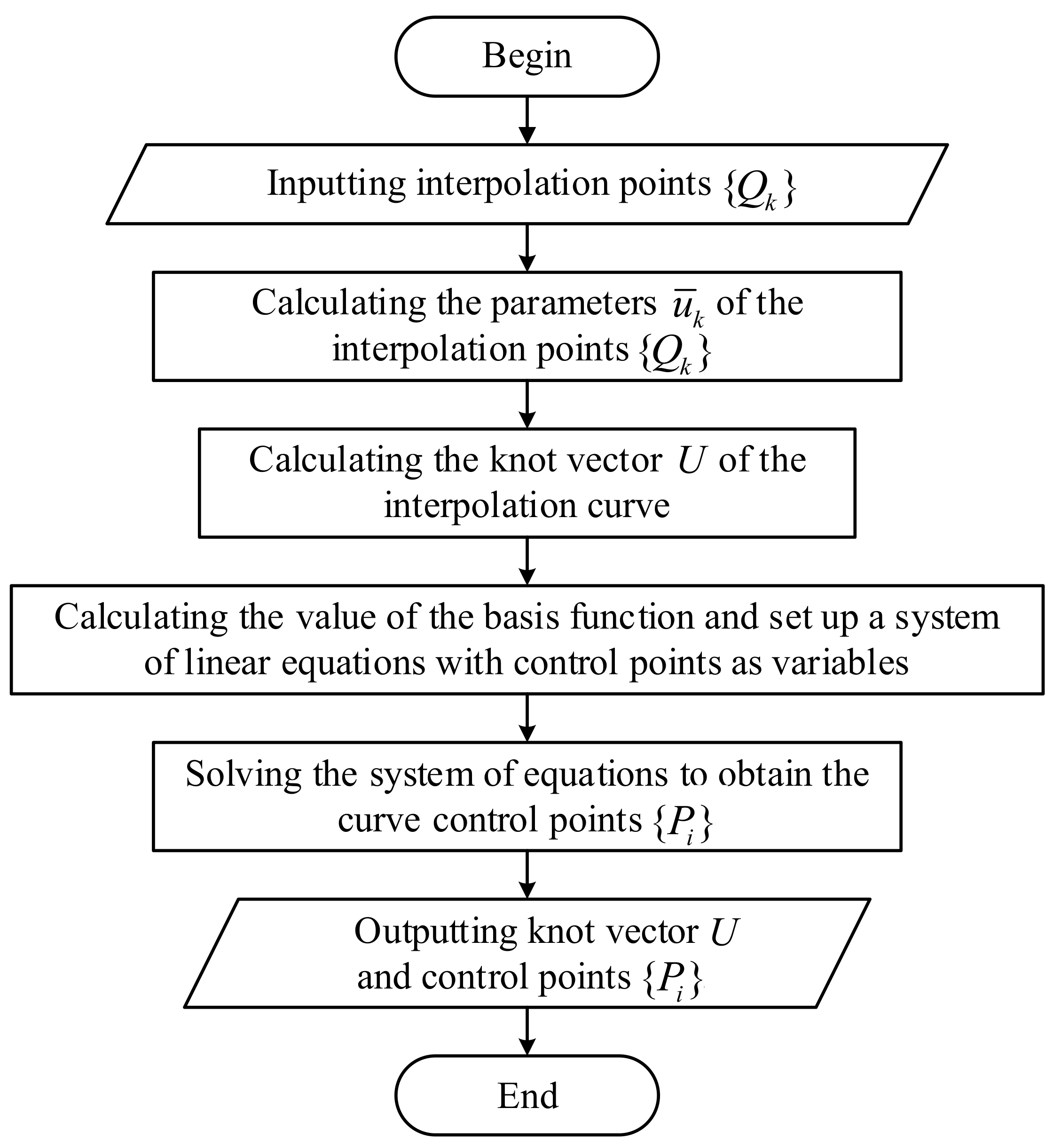
2.3. Interpolation of NURBS Curves

The process of specifying a set of data points { Q k } , k = 0 , 1 , , n and interpolating them with a pth-degree NURBS curve is called the NURBS curve interpolation.
Figure 2 shows the NURBS curve interpolation algorithm. The sample interpolation curve determines the knot vector, U, via the spatial distribution relationship of interpolating points. The control point, { P i } , is calculated by establishing a linear equation system of the coefficient matrix ( n + 1 ) × ( n + 1 ) , which is the inversion of Equation (9). The weights, { w i } , corresponding to the control points in the NURBS curve are set to 1, and the shape of the curve can be subsequently changed interactively by modifying the weights. Thus, the NURBS interpolated curve can be obtained by determining U and calculating { P i } .
Q k = C ( u ¯ k ) = i = 0 n P i N i , p ( u ¯ k ) .
The parameter u ¯ k corresponding to { Q k } can be calculated using three commonly used methods. These methods include the uniform parameterization method defined using Equation (10), the chord length parameterization method defined using Equation (11), and the centripetal parameterization method defined using Equation (12).
u ¯ k = k n , k = 1 , 2 , , n 1 u ¯ 0 = 0 u ¯ n = 1 ,
u ¯ k = u ¯ k 1 + Q k Q k 1 d , k = 1 , 2 , , n 1 u ¯ 0 = 0 u ¯ n = 1 ,
where d = k = 1 n Q k Q k 1 ;
u ¯ k = u ¯ k 1 + | Q k Q k 1 | d , k = 1 , 2 , , n 1 u ¯ 0 = 0 u ¯ n = 1 ,
where d = k = 1 n Q k Q k 1 .
U can be calculated by u ¯ k using two methods: the equidistant distribution method defined using Equation (13) and the average method defined using Equation (14). The algorithm and parameter settings are described in detail in the study by Ji et al. [47].
u 0 = = u p = 0 u m p = = u m = 1 u j + p = j n p + 1 j = 1 , 2 , , n p
u 0 = = u p = 0 u j + p = 1 p i = j j + p 1 u ¯ i , j = 1 , 2 , , n p u m p = = u m = 1 .

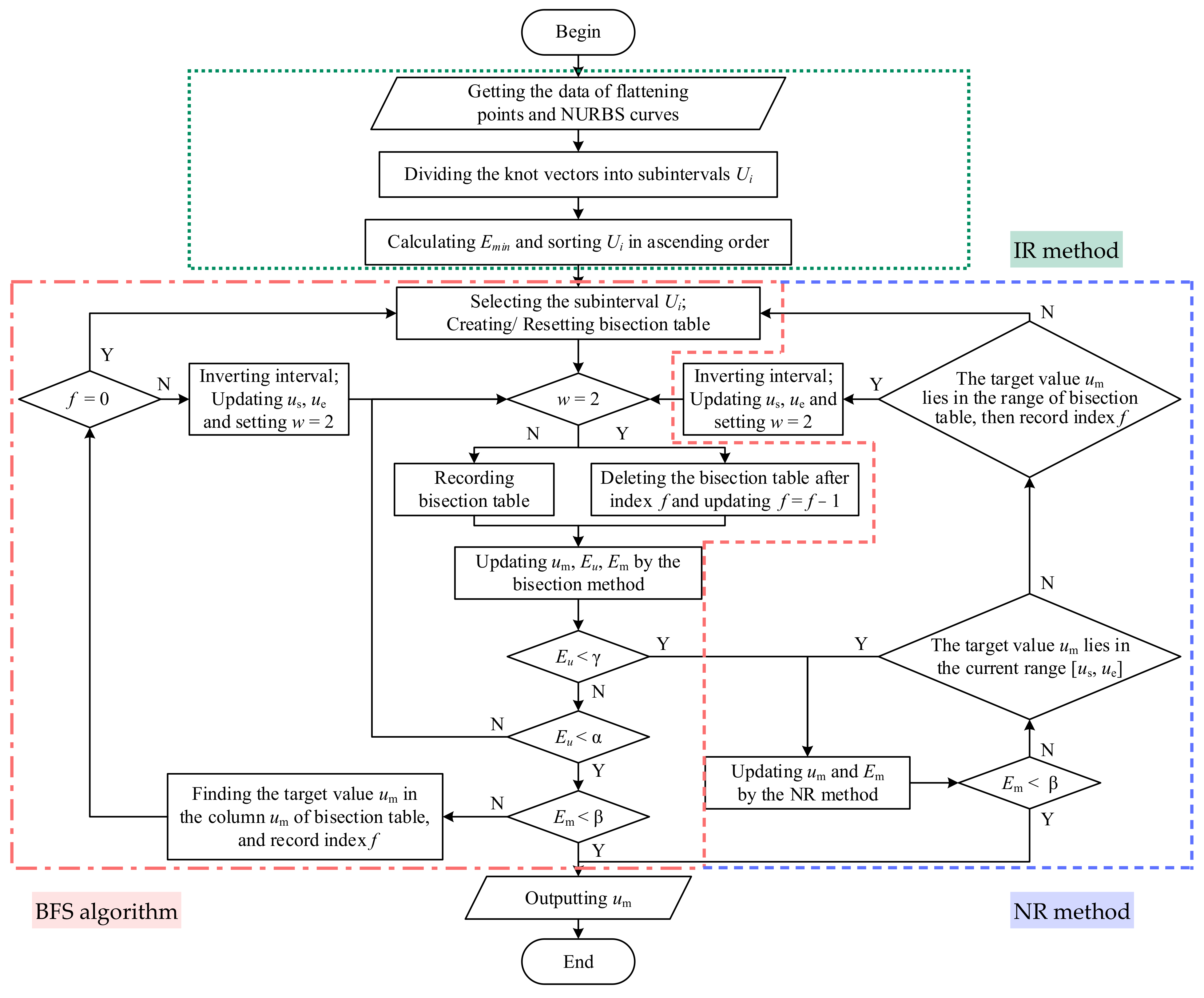
2.4. Inversion Algorithm of the NURBS Curves

The interval reformation and bisection feedback search (IR-BFS) algorithm can balance computational accuracy and efficiency in the regular precision threshold; however, its computational efficiency reduces in the high-precision threshold. This issue can be resolved using the fast high-precision bisection feedback search (FHP-BFS) algorithm, which is an improved version of the IR-BFS. The FHP-BFS algorithm introduces the NR method that facilitates its application to regular and high-precision inversion of the NURBS curve [43].
Figure 3 shows the FHP-BFS algorithm, which jumps out of the local minimum through feedback and records the iterative process of individual subintervals using feedback tables. The algorithm has three accuracy thresholds α , β , γ , where α is used to assess whether the knot interval space reaches the preset accuracy, β is used to assess whether the algorithm performs iteration on the current interval or the next subinterval, and γ is used to determine the time required for the algorithm to execute the NR method. The design and parameter setting of the FHP-BFS and IR-BFS algorithms are described in detail in the study by Zhu et al. [44].

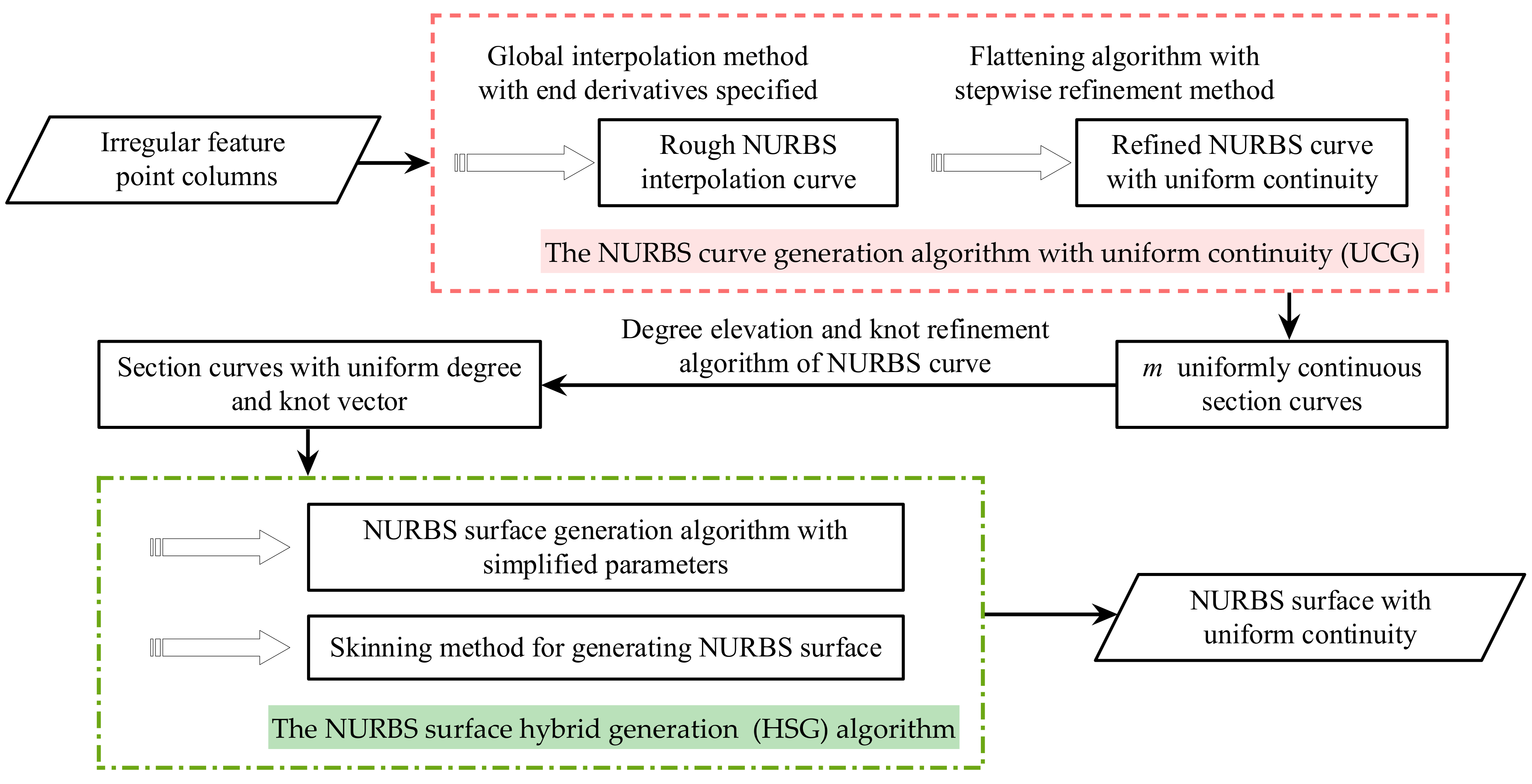
3. Framework of the Proposed Methodology

3.1. Fast Reconstruction Model with Uniform Continuity

The expression of curves or surfaces with uniform continuity refers to the mathematical model that has the same degrees of representing curves or surfaces with straight and flat parts, and their transition areas are similar. For ship hull surfaces, uniformity is a concept that refers to the mathematical representation of hull surfaces modeled holistically and uniformly and can directly avoid complicated processes, such as splicing and intersection; it is opposed to splitting amidships, bow, and stern in separate modeling methods. By generating NURBS surfaces with uniform continuity, we can study the adaptive generating sections of ship hulls and enhance computational speed by reducing the number of sections required to calculate hull stability elements. Figure 4 shows the flowchart of the fast reconstruction model of ship hull surfaces with uniform continuity.
The model includes the UCG algorithm with uniform continuity and the HSG algorithm. It fits points from the table of offsets to section curves with uniform continuity characteristics using the UCG algorithm and generates NURBS surfaces quickly using the HSG algorithm. The model is applicable to both regular and irregular feature points that can generate uniform NURBS surfaces.
The UCG algorithm considers the derivative vectors of the endpoints of the section feature points of the irregular point to generate a rough NURBS curve. At this point, the curve cannot accurately represent the straight-line segment but can only describe the curved portion of the section. Subsequently, the curve can accurately characterize the straight-line segment of the section, while preserving the original continuity, by considering a flattening algorithm with a stepwise refinement method. Cycling through the UCG algorithm results in m-section curves that accurately express the irregular feature points. The degrees and knot vectors of the uniform section curves are used as input for the HSG algorithm, which adaptively selects the NURBS surface generation algorithm based on the knot features of the section curves to improve the computational speed while ensuring accuracy. Note that a NURBS surface with uniform continuity is the output of the HSG algorithm as the generation of section curves results in the construction of NURBS curves with uniform continuity.

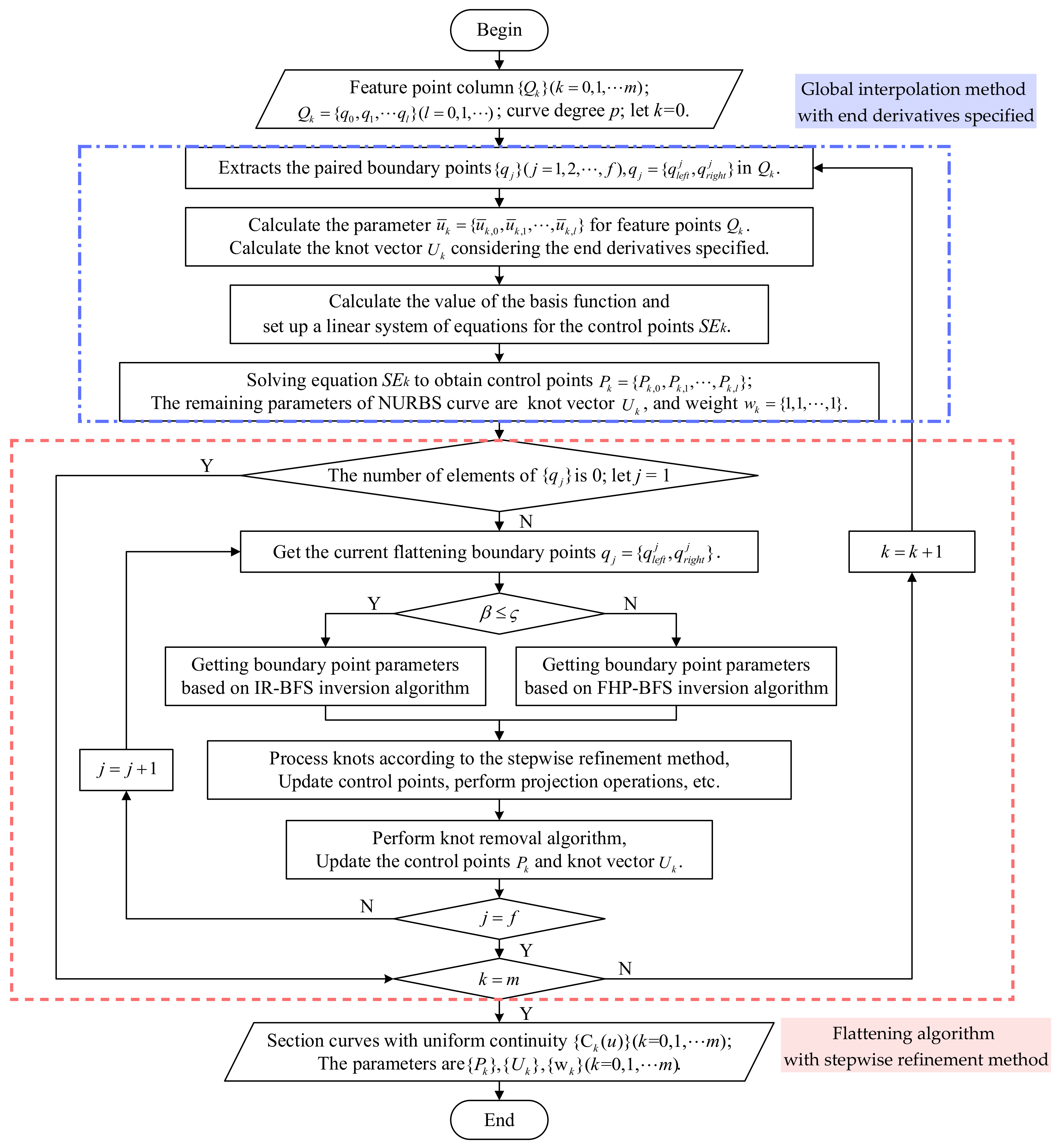
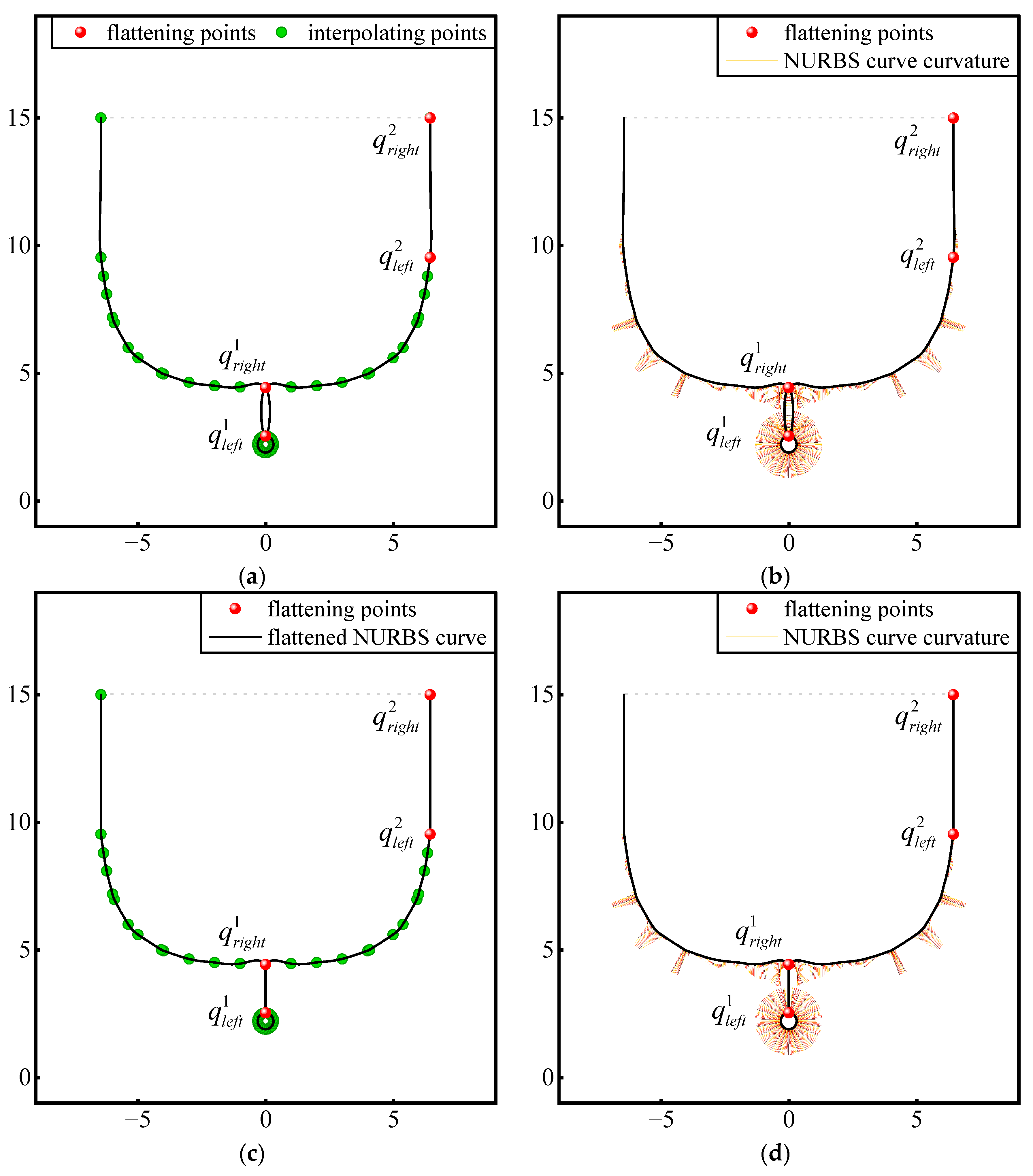
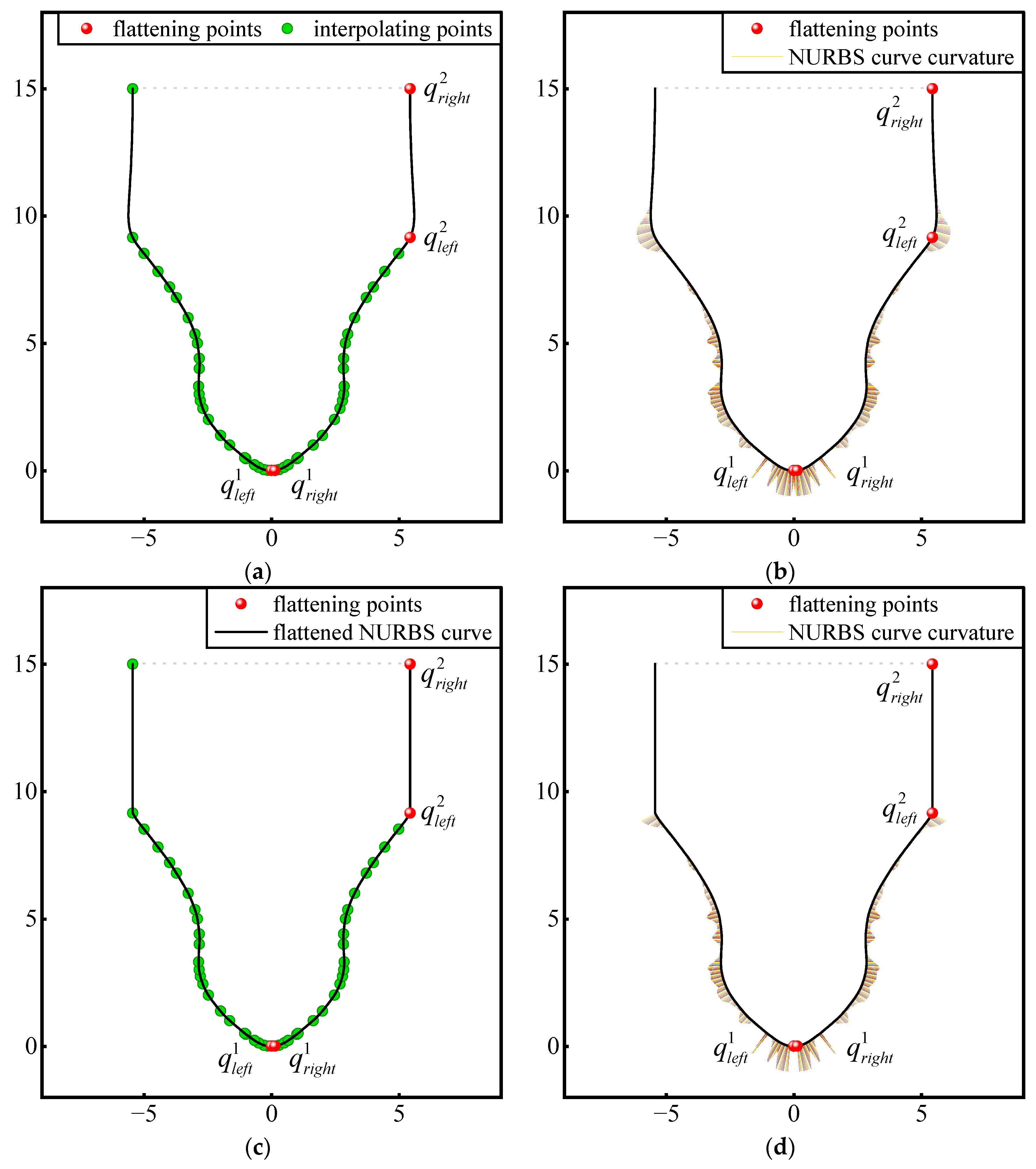
3.2. NURBS Curve Generation Algorithm with Uniform Continuity

NURBS curves with consistent continuity should be employed to achieve the NURBS surface with uniform continuity for a ship hull. This is further explained in the subsections below.

3.2.1. Framework of the UCG Algorithm

Figure 5 shows the UCG algorithm of a ship’s NURBS curve that considers the distribution characteristics of the hull profile points. The algorithm involves the generation of the fitted curve using the global interpolation method and the construction of straight-line segments using the flattening algorithm. The hull profile consists of curves and straight-line segments. In general, more straight-line segments are distributed at the endpoints of the fitted curve points in the half-width profile points. Therefore, an interpolation algorithm considering the endpoint vector is used in the global interpolation process. This design ensures the fitting accuracy of the points from the table of offsets at both ends of the curve and avoids kinked or excessively curved curves. The global interpolation algorithm is described in detail in the study by Piegl and Tiller [7].
The flattening algorithm maintains the smoothness and continuity of curves while creating straight-line segments and is improved using the stepwise knot refinement method. As depicted in Figure 6, this process gradually adds refinement knots based on the minimum number of projection points required for successful projection. When combined with the proposed knot refinement method, the flattening algorithm typically converges within two or three iterations.
Combining the flattening algorithm with the stepwise knot refinement method is associated with two challenges. First, the NURBS curve parameters of the flattening point must be obtained through inversion. Second, the impact relationships between the inserting knots in the flattening interval and the curve characteristics change should be transparent. The IR-BFS and FHP-BFS algorithms are used for the flattening algorithm to obtain the curve parameters, which enhance computational efficiency without compromising precision.

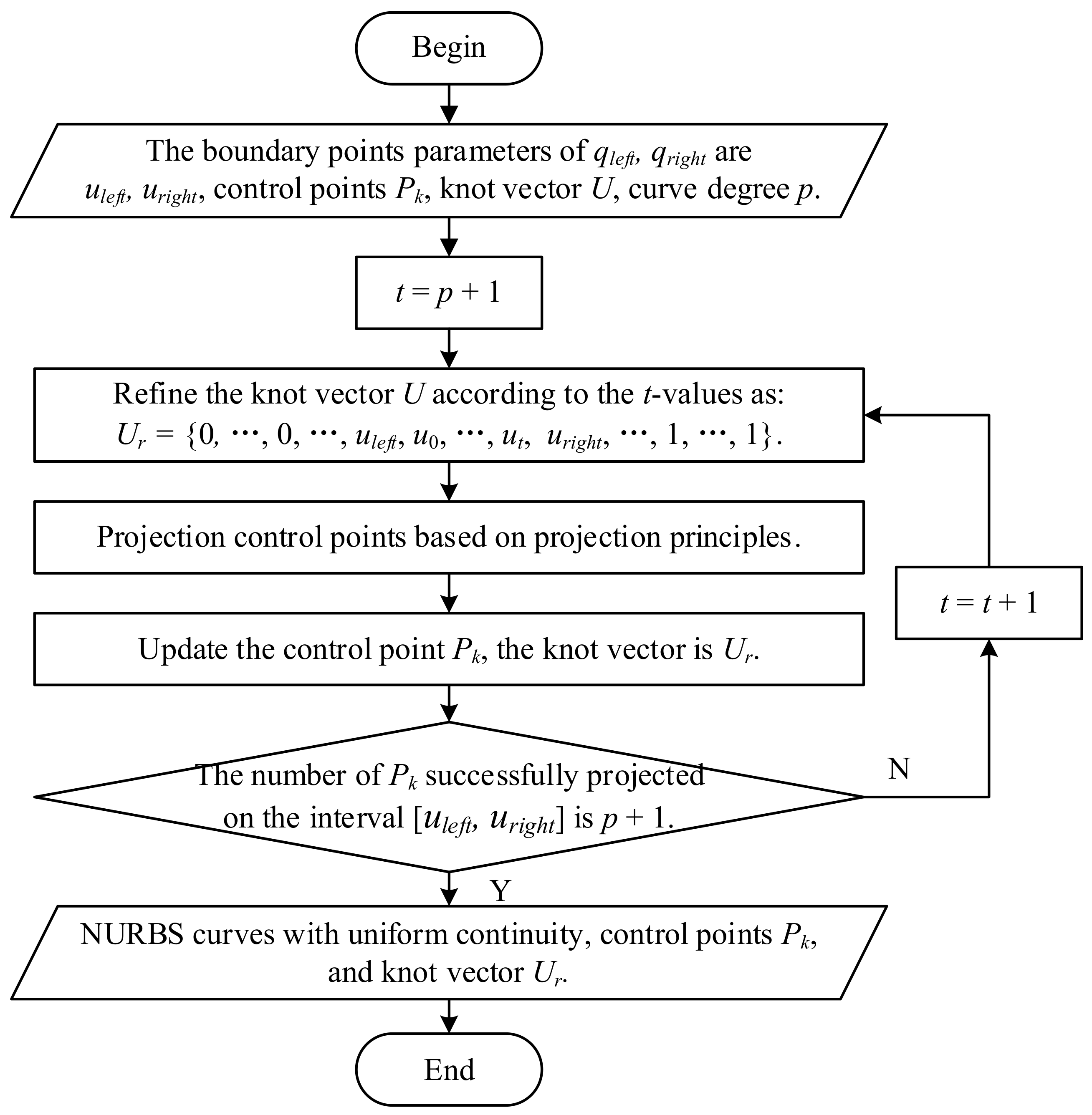
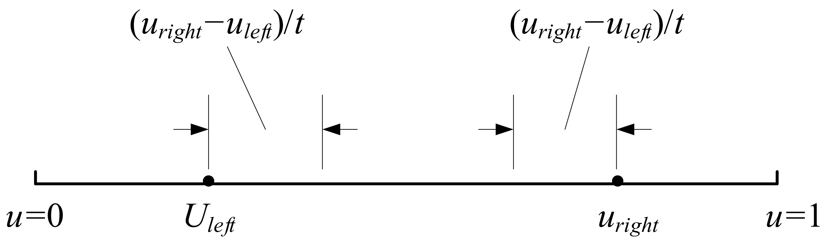
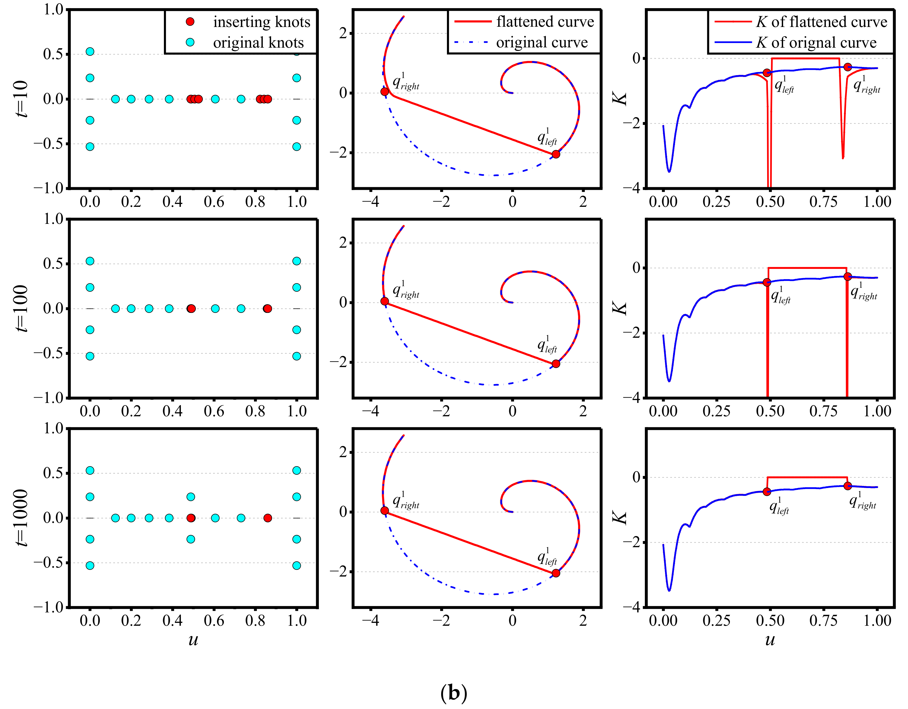
3.2.2. Parameter Setting of the Stepwise Refinement Method
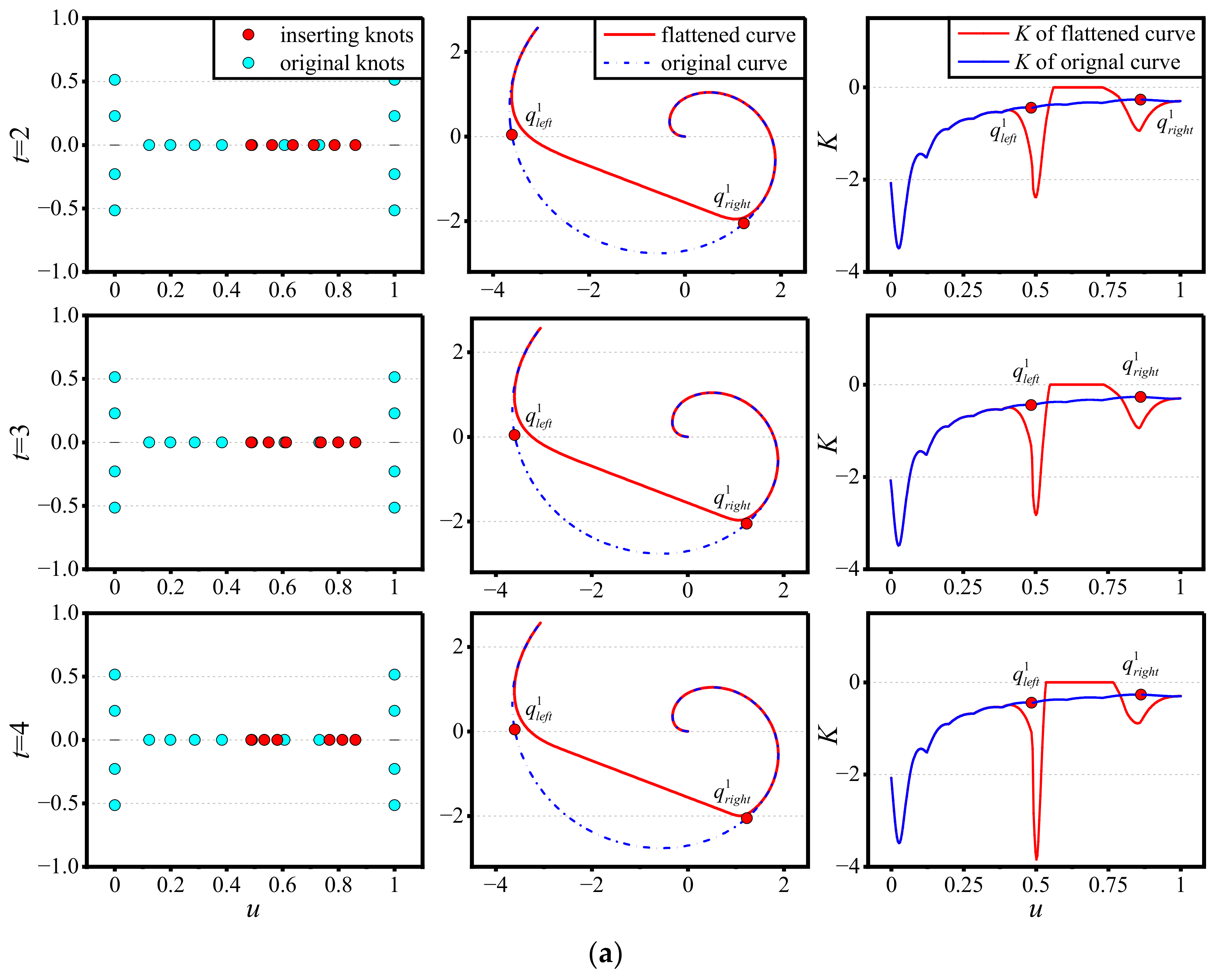
In the case of the stepwise knot refinement method applied to the flattening algorithm, different inserting knots produce different deformations to the original curve [44]. These deformations eventually affect the changes in curve curvature and other characteristics [48]. The effect of different inserting knots on the flattening curve can be obtained by conducting comparative experiments and by summarizing the optimal range of fitting parameters that meet the characteristics of the ship hull curve.
To analyze the basic concepts more clearly, geometric figures are used to describe the refinement of the knot-value problem. In Figure 7, u l e f t , u r i g h t refer to the parameters of flattening points, and ( u r i g h t - u l e f t ) / t denotes the selection interval for inserting knots. The t parameter is used to control the size of the interval, and the inserting knots are selected evenly in the interval. When t = 2 , inserting knots are selected uniformly in the interval u l e f t , u r i g h t . When t goes to infinity, inserting knots are selected in the right neighborhood of u l e f t and the left neighborhood of u r i g h t . Figure 8 shows the flattening results of inserting knots at different intervals. As shown in Figure 8a, the increase in t from 2 to 4 involves the following three features:
(i)
The inserting knots gradually approach the values of the knot parameters of flattening points;
(ii)
The smoothness of the curve near the flattening points gradually becomes less obvious;
(iii)
The curvature change speed of the flattened curves near the flattening points gradually increases.
These features are also presented in Figure 8b. When t = 1000 , the selected interval of inserting knots can be approximated as infinitesimal, and the flattened curve near the flattening points remains smooth, although the effect is not apparent. Simultaneously, the curvature changes considerably, resulting in a sudden drop to zero.
In summary, the adjustment of t can result in different flattening effects in different applications. Accuracy is paramount when creating ship surface models for performance calculations, such as ship stability. In the hull curve fitting task, the flattening point is usually also the fitting point. Hence, the flattened curve must pass through the flattening point. Therefore, t 10 3 is recommended when modeling the ship hull surface to achieve accurate curve fitting.

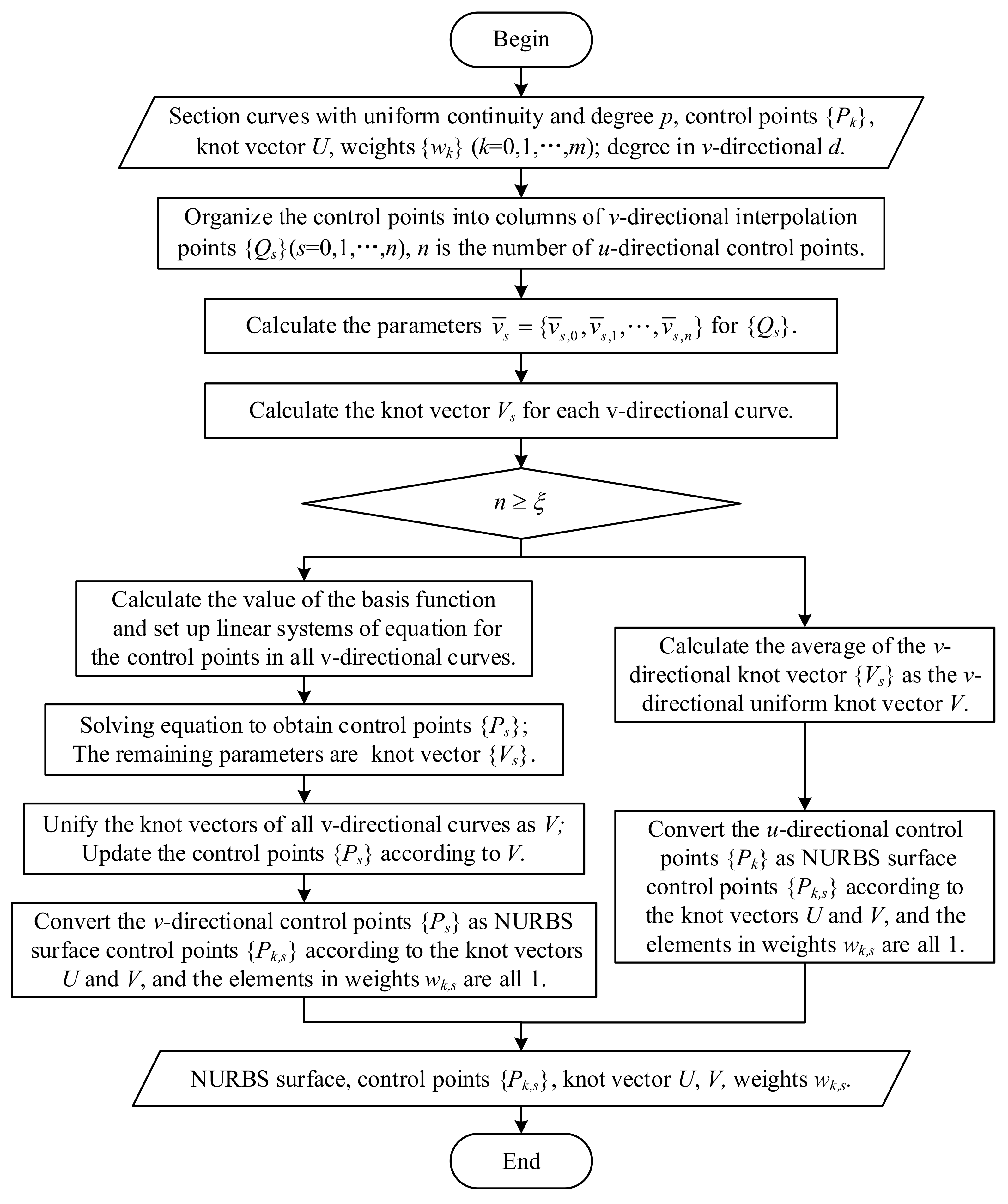
3.3. Hybrid NURBS Surface Generation Algorithm

The number of individual profile fit points in the hull profile data tends to increase with the increase in the complexity of profile features and adjacent feature variations. As shown in Figure 9, a ship has complex bow and stern profiles; thus, these positions require more fitted points from the table of offsets compared with the midship position. The use of offset data accounts for the hull shape variation in the bow and stern directions, making it easier to fit the hull profile. The curves generated from all offset data can express the hull profile and meet the requirements for fitting the hull cross-section. Moreover, the high average number of fitted points in the hull profile generates more uniform knots, simplifying the surface generation process from the section curves. Therefore, based on these features, a fast surface generation algorithm is proposed for hull NURBS.
Figure 10 shows the HSG algorithm for creating the NURBS surfaces of hulls. In this algorithm, the u-directional section curves are inputted, and the control points are arranged into a matrix of v-directional interpolation points. The interpolation algorithm acquires the knot vector, Vs, of each curve in the v-direction, while the knot vector of the section curves is already a uniform knot vector in the u-direction. The algorithm utilizes the conventional knot-generation method or the simplified knot-value method based on ξ judgment to determine all the parameters of the NURBS surface. ξ represents the threshold required for the number of control points of a single section curve in the u-direction.
In the conventional knot-generation method, the recalculation of the v-directional uniform knot vector and the updating of the related control points can generate a significant number of uniform knots and unnecessary control points. By contrast, the method of calculating the average knot value of the v-direction interpolation point matrix can be used to obtain the v-direction knot vector of the hull surface quickly. This is because the hull profile data already contain the variation pattern of hull features, and enough control points are generated in the u-direction to represent the hull profile accurately. By contrast, if the u-direction interpolation points are sparse, and the generated section curves cannot accurately express the profile features, the conventional knot-generation method should be used to improve the surface point accuracy after passing the threshold of ξ judgment. In this case, the proposed HSG algorithm can accurately represent the surface and improve computational efficiency because of the small number of knot values and control points in the u-direction that do not lead to excessive computational time consumption in the v-direction.
In addition, the ship is often associated with a discontinuous distribution of compartments in the same profile at the bow and stern, because of which the separation method is traditionally used for modeling. Therefore, the section curve with a uniform-continuity-generating method is proposed. Figure 11 shows the uniform continuity expression method for discontinuous compartments. Figure 11a shows the separated curve generation method, i.e., using two curves to fit the same profile. Figure 11b shows the proposed method for generating curves with uniform continuity that uses connection points q 1 and q 2 to reorganize the offset points so that they can construct closed curves. The duplication of the q 1 q 2 and q 2 q 1 straight-line segments will form a closed area 0 region, without affecting the values calculated for the hull elements.
In addition, the HSG algorithm is based on section curves with uniform continuity. Particularly, the curve degree needs to be unified to the highest number of section curves after interpolation to profile points. However, this process is very time-consuming. Therefore, in practice, the degree in the fitting process can be chosen directly in a uniform number to avoid the degree elevation operation and save computation time.

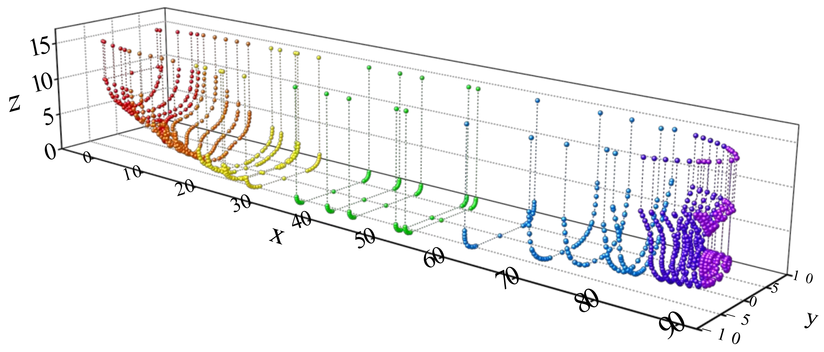
4. Results and Discussion

In this section, the effectiveness of the proposed UCG and HSG algorithms is analyzed using the offset data of a chemical ship as the sample. Figure 12 shows the spatial distribution of the scattered points of the ship hull profile and the three-dimensional display of the line connection. The hull profile stations are counted from the first station in the x-axis direction starting from the origin, and the profile data in the figure refer to 35 stations.
The experiments allowed us to examine the uniform continuity of NURBS curves generated using the UCG algorithm by analyzing the curvature change before and after the flattening operation. They also verified the effectiveness of the HSG algorithm by examining the infinite subdivision of the generated NURBS surfaces and the smoothness and continuity of subdivision profiles. Finally, the proposed hull NURBS surface generation model was compared with the existing best-performing algorithm in terms of computational efficiency. Furthermore, all the experiments were performed on a Windows 10 laptop with 32 GB RAM and a Core I7 processor using version 3.9.13 of the Python programming language and PyCharm IDE version 2022.2.4.

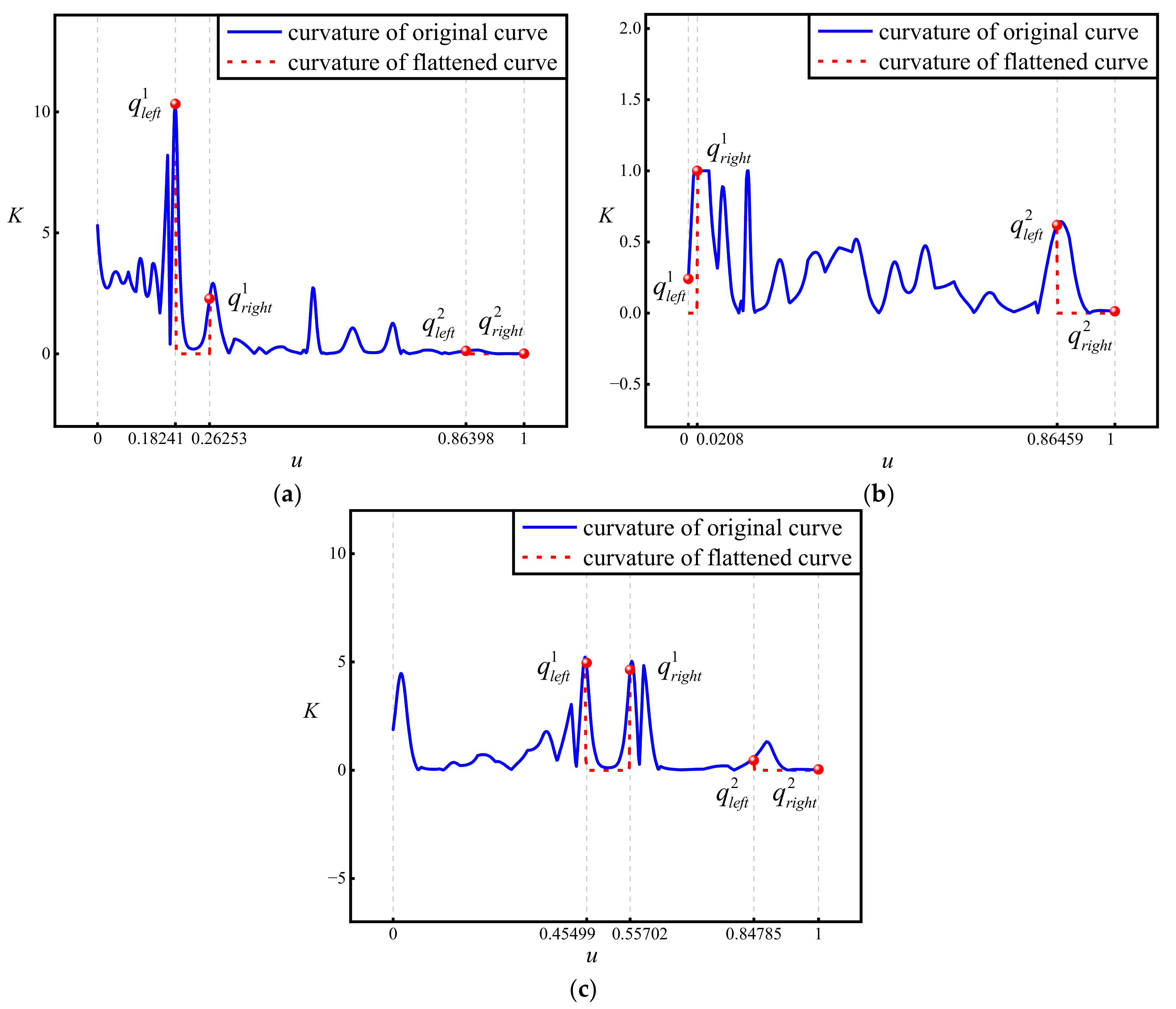
4.1. Effectiveness Analysis of the UCG Algorithm

The performance of the UCG algorithm was investigated by analyzing the process of interpolating the sample points to the initial NURBS curve generated after fitting and using the flattening algorithm to generate NURBS curves that satisfy the hull profile characteristics. Complex profiles and Stations 4, 26, and 32 near the hull bow and stern stations were finally selected to reflect the diversity of sample points and the effectiveness of the algorithm effectiveness.
The parameters involved in the experiments were set as follows: In the case of the global interpolation algorithm based on the endpoint vector values, the scattered ordered positive direction denotes the vector direction, and the size is taken as half the Euclidean distance between the endpoint and the proximity point. In the inversion algorithm, the parameters are set as α = β = 10 5 and γ = 10 3 based on the recommendation of Zhu et al. [43]. Similarly, based on the value of γ in the study by Zhu et al. [44], the parameter in the UCG algorithm is set as ς = 10 3 , t = 10 3 in the stepwise knot refinement method, and ξ = 10 3 in the HSG algorithm following a previous study [48].
Figure 13, Figure 14 and Figure 15 show the NURBS curve generation process of Stations 4, 26, and 32, respectively, and Figure 16 shows the curvature change in the curve generation process of the three stations. Figure 13a shows the NURBS curve with uniform continuity generated using the global interpolation algorithm considering the endpoint vector. The curve has two flattened straight-line segments: [ q l e f t 1 , q r i g h t 1 ] represents the straight-line segment between the stern freshwater tank and the stern tip tank profile, and [ q l e f t 2 , q r i g h t 2 ] represents the straight-line segment of the hull side. Figure 13b shows the curvature distribution porcupine of the NURBS curve in Figure 13a, and here, [ q l e f t 1 , q r i g h t 1 ] and [ q l e f t 2 , q r i g h t 2 ] are not expressed as straight sections. Figure 13c shows the NURBS curve after processing based on the flattening algorithm considering the stepwise refinement method, and the curve can be interpolated at all sample points. Figure 13d shows the porcupine plot of the curve curvature distribution of Figure 13c, where [ q l e f t 1 , q r i g h t 1 ] and [ q l e f t 2 , q r i g h t 2 ] are expressed as straight-line segments. Figure 16a shows the change in curvature before and after flattening in Figure 13. As shown in Figure 16a, the curvatures of [ q l e f t 1 , q r i g h t 1 ] and [ q l e f t 2 , q r i g h t 2 ] segments become 0 after flattening, while the rest of the curve remains unchanged; moreover, the continuity of the curve before and after flattening remains unchanged. Therefore, the NURBS curves generated using the UCG algorithm in Figure 13 have uniform continuity.
Figure 14a shows the profile curve of Station 26, which contains two flattened straight-line segments. [ q l e f t 1 , q r i g h t 1 ] represents the straight-line segment at the bottom of the hull. This station is the junction between the straight-line segment and the curve at the bottom; therefore, the length of [ q l e f t 1 , q r i g h t 1 ] is smaller. [ q l e f t 2 , q r i g h t 2 ] indicates the straight-line segment part at the side of the hull. As shown in Figure 14b, [ q l e f t 2 , q r i g h t 2 ] is not expressed as a straight-line segment. However, [ q l e f t 2 , q r i g h t 2 ] is expressed as a straight-line segment after flattening in Figure 14c,d. Figure 16b shows that the curvatures of both [ q l e f t 1 , q r i g h t 1 ] and [ q l e f t 2 , q r i g h t 2 ] segments are zero after flattening, while the rest of the curves remain unchanged.
As shown in Figure 15a, the profile curve at Station 32 includes two flattened straight-line segments. [ q l e f t 1 , q r i g h t 1 ] indicates the connection between the upper bow tip compartment and the bulbous nose bow profile, while [ q l e f t 2 , q r i g h t 2 ] indicates the straight-line section part of the hull side. Both sections are expressed as straight-line segments in Figure 15b. As shown in Figure 15c,d, the two sections are expressed as straight-line sections after flattening. Figure 16c shows that the final NURBS curve generated using the UCG algorithm for the profile of Station 32 also has uniform continuity.

4.2. Effectiveness Analysis of the HSG Algorithm

All the NURBS curves generated using the UCG algorithm were used as section curves for the generation of the HSG algorithm. The 3D wireframe plots from different viewpoints were used to check the effect of profile fitting, and the rendered plots after triangulation of the surface were used to observe the surface value distribution. The infinite subdivision of the surface and the smoothness and continuity of the subdivided surface were analyzed by determining the hull section curves with different numbers of refinement sites and displaying them as half-width profiles.
Figure 17 and Figure 18 show the 3D wireframe and surface rendering of the NURBS surface generated based on the HSG algorithm, respectively. Here, as computational parameters, 100 knots were uniformly selected in the u-direction (ship’s width direction), and 200 knots were uniformly selected in the v-direction (ship’s length direction) of the surface. The surfaces were generated using the version 3.5.3 of the Axes3D class functions in Python programming language, and the display angle was controlled by the elevation and azimuth parameters.
The surface detail fitting effect can be generally observed through the 3D wireframe view of the surface, while the distribution of the fitted values can be observed through the surface rendering view. Figure 17a shows the 3D wireframe diagram of the overall view. Each cross-section has the same x-value, and each waterline section has the same z-value. The details of the bulbous bow line are clear; the connection between the bow line and the upper part of the bowsprit can be accurately expressed as a planar connection. Moreover, the overall hull shape is smoothly expressed, and the shape of each part is smoothly connected. Figure 17b presents the details of the hull profile depression described in the profile data at Station 24 (x = 78.03). Here, the angle parameter elevation is 90, and the azimuth is 270. The bottom of the hull can be accurately represented as flat, and the bow and stern are smoothly represented. Additionally, the middle parts of the hull and the bow smoothly transition to the stern part. Figure 17c shows the elevation view, and the elevation and azimuth of the angle parameters are 270. In this figure, the bottom of the hull can be accurately expressed as a plane, the lower parts of the bow and stern are smooth, and the bottom of the hull and the bottom of the bow smoothly transition to the stern. As shown in Figure 17d, the angle parameter elevation is set to 0, and the azimuth is set to 270. Here, the stern part of the hull is smoothly expressed, the side of the hull is accurately expressed as a plane, and the transitional part of the hull is smoothly expressed in the bow, stern, and middle parts. Figure 17e,f show the right view (bow) and left view (stern), respectively. In these figures, the angle parameters are set as follows: elevation is 0, azimuth is 180, and both elevation and azimuth are set to 0. Figure 17e,f show that the hull bow and stern shapes are smooth and symmetrical and can be accurately represented.
Figure 18 shows the NURBS surface of the hull using triangulation, and the angular parameters of each view are the same as in Figure 17. The overall view of the surface is presented in Figure 18a, where the color bar color corresponds to the value of the z-axis in the hull surface. As shown in Figure 18b, the bottom of the hull is flat, and the value is close to 0. The values of the first and last parts increase smoothly from 0, and the red value is not visible in the middle part. This observation indicates that the middle part of the ship is expressed as a vertical plane, and the overall effect of fitting the ship in this view is good. As shown in Figure 18c, the bottom of the hull connecting the bottom of the bow bulb and the bottom of the stern tends to be 0, and this value continuously increases in the other directions. Here, the red value is almost invisible in the whole part of the hull. This observation indicates that the vertical part of the hull side markers can be accurately expressed, and the hull fit is good in this view. The values continuously increase from the bottom to the top of the hull, as shown in Figure 18d. Here, the bottom and top are straight-line segments, and the top part of the hull is accurately expressed as a straight-line segment, indicating that the surface boundary part is well fitted. As shown in Figure 18e,f, the values of the bow and stern of the hull are symmetrical and continuously increase from the bottom to the top, indicating that the hull is well fitted.
Figure 19 shows the half-width profile of the hull NURBS surface generated using the HSG algorithm. As shown in Figure 19a, the profile NURBS curve of the original 35 stations is obtained by interpolating the sample points in Figure 12 using the UCG algorithm.
Figure 19b shows the refined profile curve obtained by uniformly selecting 200-knot parameters from the v-direction (captain’s direction) after generating the NURBS surface using the HSG algorithm based on the original 35-station NURBS curve data. Note that an infinite number of parameters can be selected to obtain an infinitely subdivided profile curve as the NURBS surface is independent of the resolution. As shown in Figure 19b, all refinement curves have good smoothness and continuity and can reflect the details of the depression of the bow at Station 24 (x = 78.03). The comparison of Figure 19a,b indicates that all the refined curves in the transition from amidships to the stern of the bow conform to the original curve variation characteristics. Since enough knots were generated through the uniform operation in generating the hull profile curve, it can be ensured that the generalization process of the section curve in the v-direction maintains sufficient accuracy. The HSG algorithm utilizes this property to propose the uniform node method to generate surfaces with exemplary smoothness and continuity, and theoretically, it can result in infinite subdivision profiles.
In summary, the NURBS surface generated using the HSG algorithm can accurately express the characteristics of various parts of the hull, including the hull sides, details of the depression, the bottom plane and its transition, and other parts of the surface. Moreover, the algorithm fits well and features smooth shape lines and transitions in each part. Theoretically, the generated hull NURBS surface can be subdivided into infinite profiles, and the subdivided surface has good smoothness and continuity. The HSG algorithm also provides a model basis for studying the adaptive generation of the refinement sections of NURBS surfaces and considers the change in the curvature of the ship hull feature distribution.

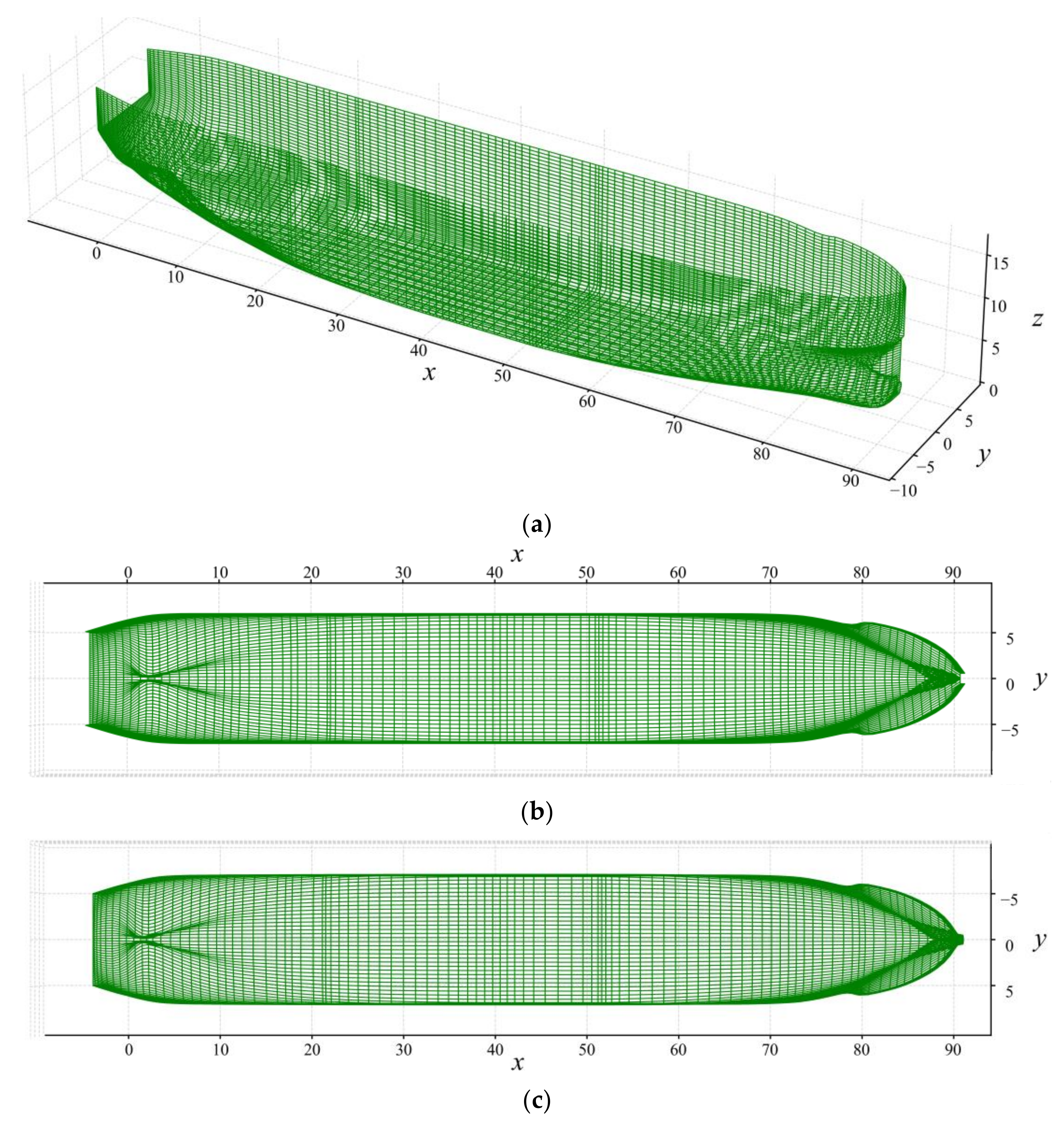
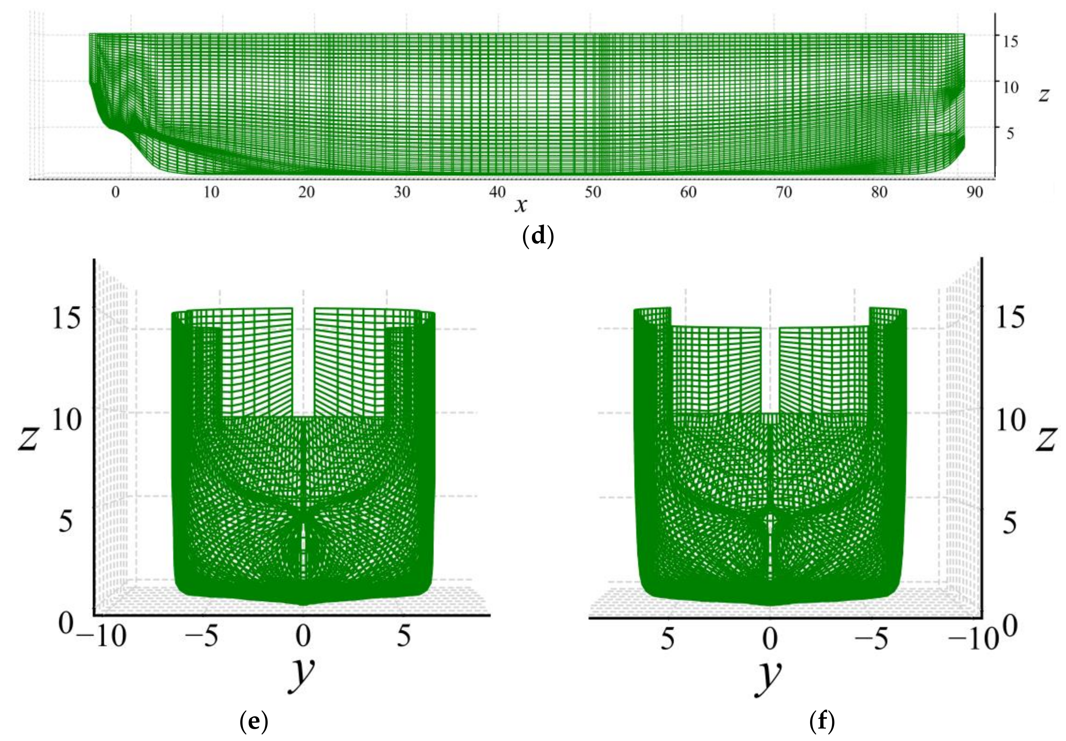
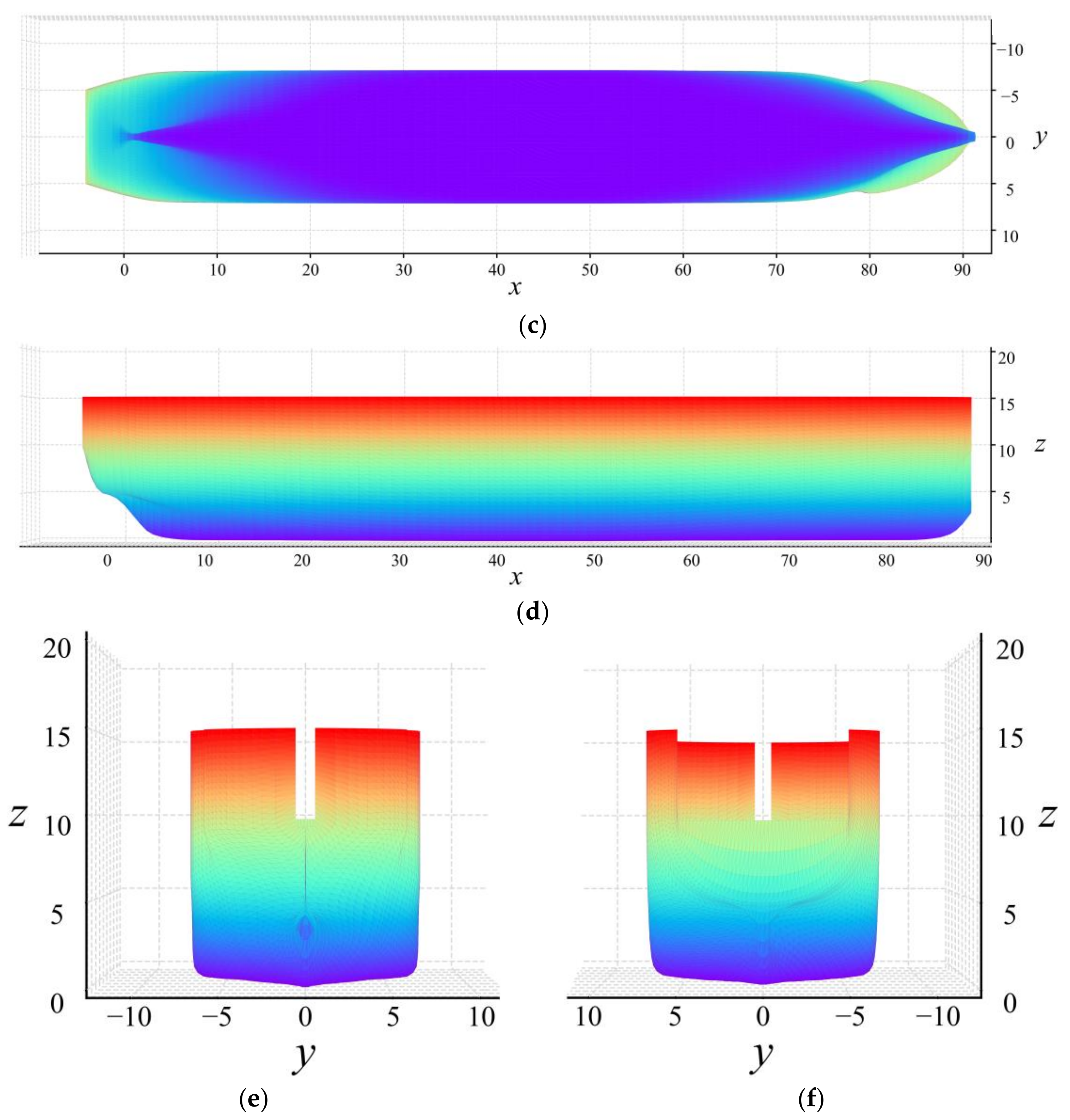
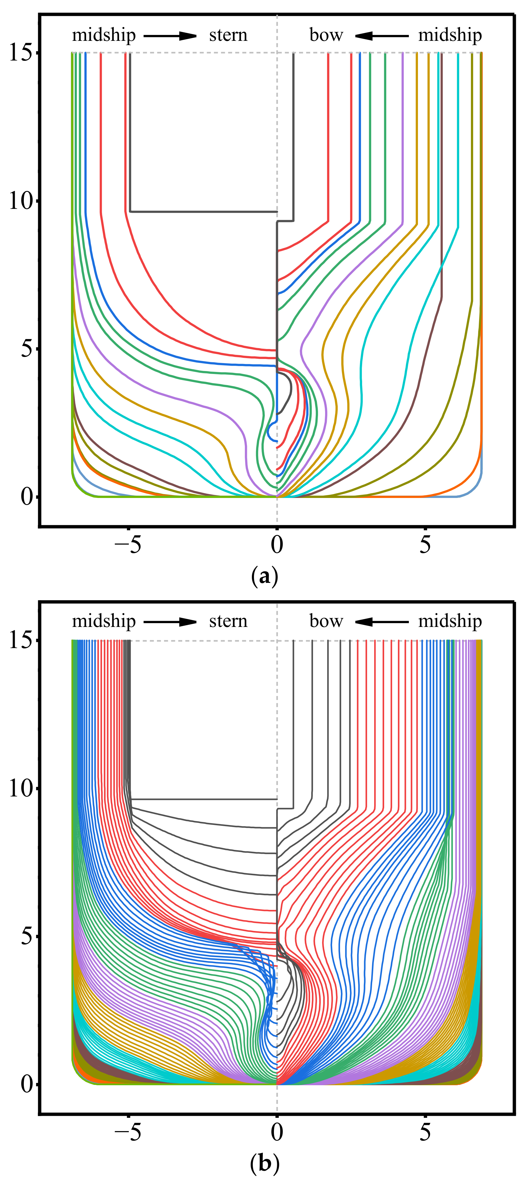
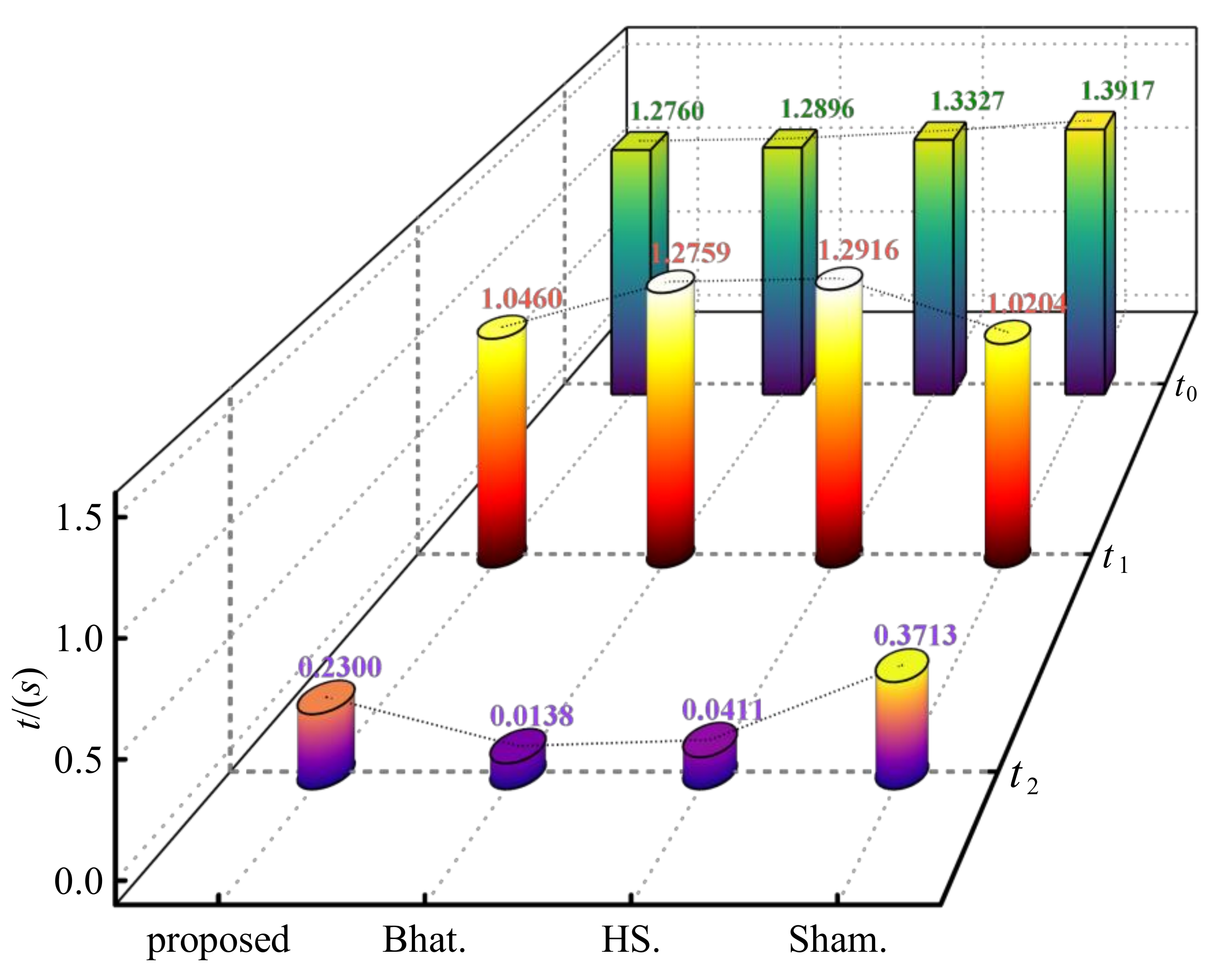
4.3. Comparison of Algorithms for Generating Ship Hull Surfaces

The speed of surface generation for the proposed model was verified through experiments based on the ship hull offset data in Figure 12 and by comparing the time consumed by all the algorithms. The following existing algorithms with the best performance in generating NURBS surfaces were selected for comparison: The algorithms proposed by Bhattarai et al. [16] and Shamsuddin et al. [22] can directly handle irregular section curves, and the algorithm proposed by He et al. [15] can directly handle regular section curves. These algorithms are abbreviated as Bhat, Sham, and HS, respectively, for convenience. The average time to generate NURBS surfaces 100 times for each algorithm was calculated using the “timeit” function in Python programming language. Here, the time taken by the algorithm to generate the surface refers to the process from processing the sample points to calculating the surface parameters. Note that processes such as those used for the surface display were excluded from this calculation.
The Bhat algorithm uses linear interpolation processing to convert irregularly interpolated samples into standard rectangular mesh data and then extracts surface control points directly. The Sham algorithm simplifies the common knot vector to reduce the number of section curve control points and thus improve the speed of surface generation. The HS algorithm uses the rectangular grid data directly; this simplifies many calculations as the global interpolation method constructs the knot vectors of the interpolation points in both directions in advance.
By combining the characteristics of each algorithm, the experimental parameters were determined, and critical processes were performed as follows: In the Bhat algorithm, the knot vector with the highest number of control points in the section curves was taken as the criterion, and the remaining curves were linearly interpolated to construct the rectangular mesh data. Additionally, all rectangular mesh points were used to construct the NURBS mesh to avoid the difference in the number of rectangular mesh points. Here, the HS algorithm was not directly applicable due to the irregular distribution of the hull profile data. In these experiments, the distribution data with rectangular grid characteristics determined using the Bhat method were used as the input data for the HS algorithm, and the data processing method was analyzed in terms of running time. Using the Sham algorithm, the five-knot vectors with the maximum number of control points were first selected. The knots were eliminated separately and then compared to check whether the final number of control points satisfied the global maximum condition. If not, the next five curves were selected, and the elimination process was repeated until the requirement would be satisfied. The curve error in the knot elimination process was set to 0.005 m, the degree of all algorithms in the u and v directions was 3, and the knot vectors in the u and v directions in Bhat’s method were set at uniform spacing following the method by Bhattarai et al. [16]. The time taken by the algorithms to calculate the parameters related to u-direction and v-direction is divided into time t1 and t2, respectively, and the total calculation time is t0. The time taken for the preparation process of each algorithm is included in time t1, which includes the time taken by the Bhat and HS algorithms to process the rectangular grid.
Figure 20 shows the computation time of each algorithm to generate the NURBS surface. In the process of t1, the HS, Bhat, proposed, and Sham algorithms take 1.2916 s, 1.2759 s, 1.046 s, and 1.0205 s, respectively. The HS algorithm has the longest calculation time, similar to the Bhat algorithm. The calculation time of Sham is the shortest, and the proposed algorithm is the second shortest. The calculation speed of the Sham and the proposed algorithm is 20.997% and 19.015% higher than that of the HS algorithm, respectively. In the t2 process, the HS, Bhat, proposed, and Sham algorithms take 0.0411 s, 0.0138 s, 0.2300 s, and 0.3713 s, respectively. The calculation time of the Sham algorithm is the longest, and the proposed algorithm is the second longest. The calculation time of the Bhat and HS algorithms is shorter. Compared with the Sham algorithm, the computing speed of the Bhat, HS, and the proposed algorithm is increased by 96.283%, 88.931%, and 38.055%, respectively. In the t0 process, the HS, Bhat, proposed, and Sham algorithms take 1.3327 s, 1.2896 s, 1.2760 s, and 1.3917 s, respectively. The Sham algorithm has the most computing time, while the proposed algorithm has the least. Compared with the Sham, HS, and Bhat algorithms, the computing speed of the proposed algorithm increased by 8.314%, 4.255%, and 1.055%, respectively. In summary, the calculation speed of the proposed algorithm can be increased by up to 8.314% compared with the comparison algorithms.
In the Bhat and HS algorithms, t1 includes the time it takes to integrate the interpolated points into a rectangular grid. However, the HS algorithm calculates the knot vectors and control points via global interpolation; therefore, the computation time in t1 is slightly longer. In comparison, the Bhat algorithm directly extracts the rectangular grid as control points and performs uniform interpolation to construct the two directional knot vectors, saving some computation time. The same is true for t2. The direct construction of uniform interpolation points saves a considerable amount of computation time for the Bhat algorithm; however, the algorithm does not consider the distribution characteristics of the interpolation points. Here, the constructed surface was relatively rough, even though the computation was fast. Additionally, the details of the transition between straight-line segments and curves in the hull surface are difficult to describe accurately. The Sham algorithm and the proposed algorithms take relatively the same amount of time in the t1 and t2 stages. Note that the Sham algorithm may consume too much time in constructing simplified common knot vectors in the t1 and t2 processes due to the uncertainty involved in the knot elimination process. The proposed algorithm obtains the surface parameters via global interpolation and flattening operations in the t1 process, which is more stable, while in its t2 process, the average knot method is used to fit the control points and improve the computational speed. The proposed algorithm takes much more computational time than the Bhat and HS algorithms due to the numerous v-directional interpolation curves. However, this is expected as it generates more realistic surface accuracy and feature point distribution and thus requires a certain amount of time.
In summary, the proposed model exhibits the best performance in generating NURBS surfaces among the compared algorithms while considering the interpolation point distribution characteristics and relevant details. The proposed model can provide a research basis for the real-time calculation of hydrostatic elements for offshore damaged ships.

5. Conclusions

In this study, we investigated how to quickly construct ship hull NURBS surfaces suitable for the calculation of hydrostatic elements for damaged ships. First, we proposed an algorithm for generating NURBS curves with uniform continuity by fusing the global interpolation and flattening algorithms, i.e., the UCG algorithm. Then, we constructed an accurate and fast NURBS surface generation algorithm, i.e., the HSG algorithm, by fusing the number of common knots of section curves. We also performed experiments to examine the uniform continuity and accuracy of generating curves and surfaces and verified the computational efficiency of the surface generation model by comparing it with other algorithms. The comparison results show that the total calculation time of HS [15], Bhat [16], proposed, and Sham [22] algorithms are 1.3327 s, 1.2896 s, 1.2760 s, and 1.3917 s, respectively. Therefore, compared with other algorithms, the computational speed of the proposed algorithm is increased by 8.314%, 4.255%, and 1.055%, respectively; that is, the maximum increase can be 8.314%.
The main contributions of this study are as follows:
(i)
A UCG algorithm was proposed for the fast generation of NURBS curves with uniform continuity that can accurately express hull bending and planar details. The proposed algorithm generates accurate hull NURBS curves from the table of offsets or waterline data by considering the feature distribution of a hull profile.
(ii)
An HSG algorithm adapted to the UCG algorithm was proposed to improve the calculation speed while guaranteeing the accuracy of the ship hull NURBS surface.
(iii)
The combination of the UCG and HSG algorithms can construct a fast-generation algorithm for hull NURBS surfaces with uniform continuity. The optimal selection range of relevant parameters of the UCG algorithm was determined with comparison experiments, facilitating its application to engineering and other similar studies.
Based on our findings, the proposed model can greatly improve the speed and accuracy of generating NURBS surfaces with uniform continuity. This model can be utilized for the adaptive calculation of elements while considering the variation in surface curvature [49] and hydrodynamic calculation [50]. It also enhances the efficiency of real-time calculation tasks based on ship hull compartments.
Note that the proposed algorithms and model were tested utilizing chemical ship data. Thus, more ship data should be incorporated in the future to obtain more reliable and generalized experimental results. Future studies should also investigate the application of this algorithm in calculating ship hull and compartment surface elements, considering the thickness of hull plates.

Author Contributions

K.Z.: conceptualization, methodology, software, formal analysis, writing—original draft preparation, writing—review and editing. G.S.: supervision. J.L.: software, writing—review and editing. J.S.: writing—review and editing. All authors have read and agreed to the published version of the manuscript.

Funding

This work was supported by the National Natural Science Foundation of China (52201414), the Provincial Natural Science Foundation of Liaoning (20170540090), and the Navigation College of Dalian Maritime University.

Institutional Review Board Statement

Not applicable.

Informed Consent Statement

Not applicable.

Data Availability Statement

The data presented in this study are available on request from the corresponding author.

Acknowledgments

The authors are grateful for the support of the Key Laboratory of Navigation Safety Guarantee of Liaoning Province, China.

Conflicts of Interest

The authors declare no conflict of interest.

References

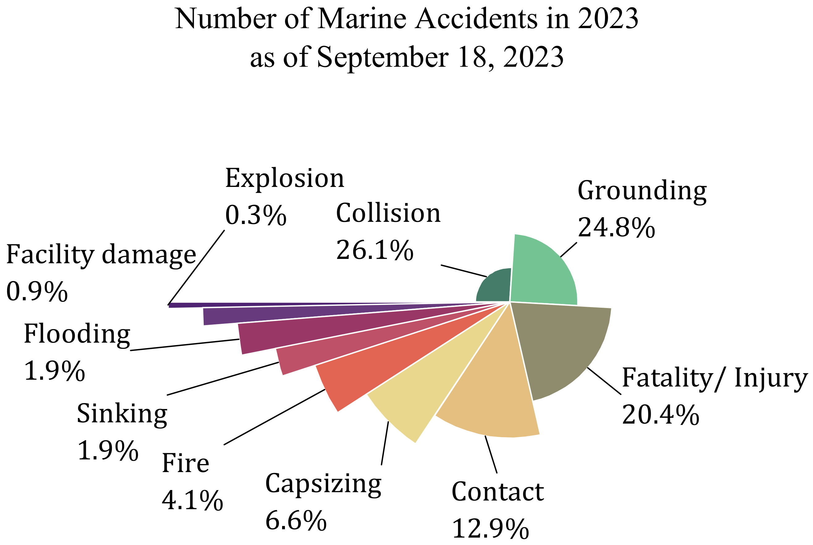
  1. Japan Transport Safety Board (JTSB). Statistics of Marine Accidents and Incidents. Available online: https://www.mlit.go.jp/jtsb/statistics_mar.html (accessed on 13 September 2023).
  2. European Maritime Safety Agency (EMSA). EMSA Facts and Figures 2022; European Maritime Safety Agency: Lisbon, Portugal, 2023; Available online: http://www.emsa.europa.eu/ (accessed on 19 May 2023).
  3. Sun, X.; Ni, Y.; Liu, C.; Wang, Z.; Yin, Y. A practical method for stability assessment of a damaged ship. Ocean Eng. 2021, 222, 108594. [Google Scholar] [CrossRef]
  4. Asadi, P.; Alimohammadi, S.; Kohantorabi, O. Effects of material type, preheating and weld pass number on residual stress of welded steel pipes by multi-pass TIG welding. Therm. Sci. Eng. Progress 2020, 16, 100462. [Google Scholar] [CrossRef]
  5. Akbari, M.; Asadi, P. Dissimilar friction stir lap welding of aluminum to brass: Modeling of material mixing using coupled Eulerian–Lagrangian method with experimental verifications. Proc. Inst. Mech. Eng. Part L J. Mater. Des. Appl. 2020, 234, 1117–1128. [Google Scholar] [CrossRef]
  6. Jung, H.B.K.; Kim, K. A new parameterisation method for NURBS surface interpolation. Int. J. Adv. Manuf. Technol. 2000, 16, 784–790. [Google Scholar] [CrossRef]
  7. Piegl, L.; Tiller, W. The NURBS Book, 2nd ed.; Springer: Berlin/Heidelberg, Germany, 1996. [Google Scholar]
  8. Kulczycka, M.A.; Nachman, L.J. Qualitative and quantitative comparisons of B-spline offset surface approximation methods. Comput.-Aided Des. 2002, 34, 19–26. [Google Scholar] [CrossRef]
  9. Park, H.; Kim, K.; Lee, S.C. A method for approximate NURBS curve compatibility based on multiple curve refitting. Comput.-Aided Des. 2000, 32, 237–252. [Google Scholar] [CrossRef]
  10. Piegl, L.; Tiller, W. Algorithm for approximate NURBS skinning. Comput.-Aided Des. 1996, 28, 699–706. [Google Scholar] [CrossRef]
  11. Andradas, C.; Recio, T.; Sendra, J.R.; Tabera, L.F.; Villarino, C. Reparametrizing swung surfaces over the reals. Appl. Algebra Eng. Commun. Comput. 2014, 25, 39–65. [Google Scholar] [CrossRef]
  12. Farouki, R.T.; Nittler, K.M. Rational swept surface constructions based on differential and integral sweep curve properties. Comput. Aided Geom. Des. 2015, 33, 1–16. [Google Scholar] [CrossRef]
  13. Boden, H.U.; Chrisman, M.; Karimi, H. The Gordon-Litherland pairing for links in thickened surfaces. Int. J. Math. 2022, 33, 2250078. [Google Scholar] [CrossRef]
  14. Randrianarivony, M. On global continuity of Coons mappings in patching CAD surfaces. Comput.-Aided Des. 2009, 41, 782–791. [Google Scholar] [CrossRef]
  15. He, S.; Xuan, J.; Du, W.; Xia, Q.; Xiong, S.; Zhang, L.; Wang, Y.; Wu, J.; Tao, H.; Shi, T. Spiral tool path generation method in a NURBS parameter space for the ultra-precision diamond turning of freeform surfaces. J. Manuf. Process. 2020, 60, 340–355. [Google Scholar] [CrossRef]
  16. Bhattarai, S.; Dahal, K.; Vichare, P.; Chen, W. Adapted Delaunay triangulation method for free-form surface generation from random point clouds for stochastic optimization applications. Struct. Multidiscip. Optim. 2020, 61, 649–660. [Google Scholar] [CrossRef]
  17. Park, H.; Kim, K. Smooth surface approximation to serial cross-sections. Comput.-Aided Des. 1996, 28, 995–1005. [Google Scholar] [CrossRef]
  18. Park, H. An approximate lofting approach for B-spline surface fitting to functional surfaces. Int. J. Adv. Manuf. Technol. 2001, 18, 474–482. [Google Scholar] [CrossRef]
  19. Piegl, L.A.; Tiller, W. Surface skinning revisited. Vis. Comput. 2002, 18, 273–283. [Google Scholar] [CrossRef]
  20. Piegl, L.A.; Tiller, W. Biarc approximation of NURBS curves. Comput.-Aided Des. 2002, 34, 807–814. [Google Scholar] [CrossRef]
  21. Park, H. Lofted B-spline surface interpolation by linearly constrained energy minimization. Comput.-Aided Des. 2003, 35, 1261–1268. [Google Scholar] [CrossRef]
  22. Shamsuddin, S.M.; Ahmed, M.A.; Smian, Y. NURBS skinning surface for ship hull design based on new parameterization method. Int. J. Adv. Manuf. Technol. 2006, 28, 936–941. [Google Scholar] [CrossRef]
  23. Shamsuddin, S.M.H.; Ahmed, M.A. A hybrid parameterization method for NURBS. In Proceedings of the International Conference on Computer Graphics, Imaging and Visualization 2004, Penang, Malaysia, 2 July 2004; pp. 15–20. [Google Scholar]
  24. Wu, H. An adaptive character skinning algorithm based on the property of real skin. Comput. Anim. Virtual Worlds 2019, 30, e1868. [Google Scholar] [CrossRef]
  25. Bang, S.; Lee, S.H. Spline interface for intuitive skinning weight editing. ACM Trans. Graph. 2018, 37, 1–14. [Google Scholar] [CrossRef]
  26. Yin, H.; Mukundan, R. Improved vertex skinning algorithm based on dual quaternions. In Proceedings of the 2019 IEEE 21st International Workshop on Multimedia Signal Processing (MMSP), Kuala Lumpur, Malaysia, 27–29 September 2019; pp. 1–6. [Google Scholar]
  27. Liu, S.L.; Liu, Y.; Dong, L.F.; Tong, X. RAS: A data-driven rigidity-aware skinning model for 3D facial animation. Comput. Graph. Forum 2020, 39, 581–594. [Google Scholar] [CrossRef]
  28. Moutafidou, A.; Toulatzis, V.; Fudos, I. Temporal parameter-free deep skinning of animated meshes. In Advances in Computer Graphics; Springer: Cham, Switzerland, 2021; pp. 3–24. [Google Scholar]
  29. Kruppa, K.; Kunkli, R.; Hoffmann, M. A skinning technique for modeling artistic disk B-spline shapes. Comput. Graph. 2023, 115, 96–106. [Google Scholar] [CrossRef]
  30. Wei, J.; Sun, C.; Zhang, X.J.; Wang, E.J.; Law, D. An efficient and accurate interpolation method for parametric curve machining. Sci. Rep. 2022, 12, 16000. [Google Scholar] [CrossRef] [PubMed]
  31. Ma, W.; Kruth, J.P. Parametrization of randomly measured points for least- squares fitting of B-spline curves and surfaces. Comput.-Aided Des. 1995, 27, 663–675. [Google Scholar] [CrossRef]
  32. Xiao, Y.J.; Li, Y.F. Optimized stereo reconstruction of free-form space curves based on a non-uniform rational B-spline model. J. Opt. Soc. Am. A Opt. Image Sci. Vis. 2005, 22, 1746–1762. [Google Scholar] [CrossRef] [PubMed]
  33. Saini, D.; Kumar, S.; Gulati, T.R. NURBS-based geometric inverse reconstruction of free-form shaped objects. JKSU-Comput. Inf. Sci. 2017, 29, 116–133. [Google Scholar]
  34. Vahdani, R.; Saraee, S.M.; Mohtashami, V. Parallel body-shaping of electrically large objects described by NURBS surfaces. Int. J. RF Microw. Comput. Aid Eng. 2022, 32, e23543. [Google Scholar] [CrossRef]
  35. Voisin, S.; Abidi, M.A.; Foufou, S.; Truchetet, F. Genetic algorithms for 3D reconstruction with supershapes. In Proceedings of the 2009 16th IEEE International Conference on Image Processing (ICIP), Cairo, Egypt, 7–10 November 2009; pp. 529–532. [Google Scholar]
  36. Cai, Y.; Su, Z.; Li, Z.; Sun, R.; Liu, X.; Zhao, Y. Two-view curve reconstruction based on the snake model. J. Comput. Appl. Math. 2011, 236, 631–639. [Google Scholar] [CrossRef]
  37. Saini, D.; Kumar, S.; Gulati, T.R. Reconstruction of free-form space curves using NURBS-snakes and a quadratic programming approach. Comput. Aided Geom. Des. 2015, 33, 30–45. [Google Scholar] [CrossRef]
  38. Lu, Y.; Yong, J.H.; Shi, K.L.; Song, H.C.; Ye, T.Y. 3D B-spline curve construction from orthogonal views with self-overlapping projection segments. Comput. Graph. 2016, 54, 18–27. [Google Scholar] [CrossRef]
  39. Alazzam, A.; Alomar, B. Using average uniform algorithm to model educational data. In Proceedings of the 2017 Fourth HCT Information Technology Trends (ITT), Al Ain, United Arab Emirates, 25–26 October 2017; IEEE: New York, NY, USA, 2017; pp. 30–34. [Google Scholar]
  40. Singh, A.; Deep, K. Reconstruction of 3D curves and surfaces using new variants of gravitational search algorithm. J. Inf. Optim. Sci. 2018, 39, 1199–1221. [Google Scholar] [CrossRef]
  41. Saini, D.; Kumar, S.; Singh, M.K.; Ali, M. Two view NURBS reconstruction based on GACO model. Complex. Intell. Syst. 2021, 7, 2329–2346. [Google Scholar] [CrossRef]
  42. Wang, Z.; Cao, Z.; Fan, F.; Sun, Y. Shape optimization of free-form grid structures based on the sensitivity hybrid multi-objective evolutionary algorithm. J. Build. Eng. 2021, 44, 102538. [Google Scholar] [CrossRef]
  43. Zhu, K.; Shi, G.; Liu, J.; Shi, J. Fast high-precision bisection feedback search algorithm and its application in flattening the NURBS curve. J. Mar. Sci. Eng. 2022, 10, 1851. [Google Scholar] [CrossRef]
  44. Zhu, K.G.; Shi, G.Y.; Liu, J. Improved flattening algorithm for NURBS curve based on bisection feedback search algorithm and interval reformation method. Ocean Eng. 2022, 247, 110635. [Google Scholar] [CrossRef]
  45. Hughes, T.J.R.; Cottrell, J.A.; Bazilevs, Y. Isogeometric analysis: CAD, finite elements, NURBS, exact geometry and mesh refinement. Comput. Methods Appl. Mech. Eng. 2005, 194, 4135–4195. [Google Scholar] [CrossRef]
  46. Arapakopoulos, A.; Polichshuk, R.; Segizbayev, Z.; Ospanov, S.; Ginnis, A.I.; Kostas, K.V. Parametric models for marine propellers. Ocean Eng. 2019, 192, 106595. [Google Scholar] [CrossRef]
  47. Ji, S.; Lei, L.; Zhao, J.; Lu, X.; Gao, H. An adaptive real-time NURBS curve interpolation for 4-axis polishing machine tool. Robot. Comput.-Integr. Manuf. 2021, 67, 102025. [Google Scholar] [CrossRef]
  48. Zhu, K.; Shi, G.; Liu, J. Fast NURBS Skinning Algorithm and Ship Hull Section Refinement Model. In Proceedings of the 2023 7th International Conference on Machine Learning and Soft Computing (ICMLSC’23), Chongqing, China, 5–7 January 2023; Association for Computing Machinery: New York, NY, USA, 2023; pp. 26–33. [Google Scholar]
  49. Callens, S.J.P.; Uyttendaele, R.J.C.; Fratila-Apachitei, L.E. Substrate curvature as a cue to guide spatiotemporal cell and tissue organization. Biomaterials 2019, 232, 119739. [Google Scholar] [CrossRef] [PubMed]
  50. Zhang, L.; Shi, W.; Karimirad, M. Second-order hydrodynamic effects on the response of three semisubmersible floating offshore wind turbines. Ocean Eng. 2020, 207, 107371. [Google Scholar] [CrossRef]
Figure 1. Statistics of marine accidents according to the Japan Transport Safety Board.
Jmse 11 01816 g001
Figure 2. Flowchart of the NURBS curve interpolation algorithm.
Jmse 11 01816 g002
Figure 3. Flowchart of the fast high-precision bisection feedback search (FHP-BFS) algorithm.
Jmse 11 01816 g003
Figure 4. Fast NURBS surface generation model of ship hull with uniform continuity.
Jmse 11 01816 g004
Figure 5. Ship NURBS curve generation algorithm with uniform continuity (UCG).
Jmse 11 01816 g005
Figure 6. Stepwise knot refinement method in flattening algorithm.
Jmse 11 01816 g006
Figure 7. Range of selecting inserting knots, where us and ue denote the flattening points, and t is the parameter that affects the range’s size.
Jmse 11 01816 g007
Figure 8. Flattening results with different inserting ranges: (a) t = 2, 3, and 4; (b) t = 10, 100, and 1000.
Jmse 11 01816 g008aJmse 11 01816 g008b
Figure 9. Point and line diagram of the hull half-width profile points.
Jmse 11 01816 g009
Figure 10. Hybrid NURBS surface generation (HSG) algorithm.
Jmse 11 01816 g010
Figure 11. Point and line diagram of the discontinuous compartment expressing method with uniform continuity: (a) separated section curve generation method; (b) section curve obtained using the uniform-continuity-generating method, where q 1 and q 2 are the connecting points.
Jmse 11 01816 g011
Figure 12. Point–line diagram of the 3D profile in the table of offsets of a ship hull.
Jmse 11 01816 g012
Figure 13. Process of NURBS curve generation of Station 4 using the UCG algorithm: (a) NURBS curve generated using the interpolation algorithm considering the endpoint vector; (b) porcupine plot of the NURBS curve in (a); (c) flattened NURBS curve of (a) using the flattening algorithm considering the stepwise refinement method; (d) porcupine plot of the NURBS curve in (c).
Jmse 11 01816 g013
Figure 14. Process of NURBS curve generation of Station 26 using the UCG algorithm: (a) NURBS curve generated by the interpolation algorithm considering the endpoint vector; (b) porcupine plot of the NURBS curve in (a); (c) flattened NURBS curve of (a) generated by the flattening algorithm considering the stepwise refinement method; (d) porcupine plot of the NURBS curve in (c).
Jmse 11 01816 g014
Figure 15. Process of NURBS curve generation of Station 32 using the UCG algorithm: (a) NURBS curve generated by the interpolation algorithm considering the endpoint vector; (b) porcupine plot of the NURBS curve in (a); (c) flattened NURBS curve of (a) generated by the flattening algorithm considering the stepwise refinement method; (d) porcupine plot of the NURBS curve in (c).
Jmse 11 01816 g015
Figure 16. Change in the curvature of the NURBS curve before and after flattening via the UCG algorithm: (a) Station 4; (b) Station 26; (c) Station 32.
Jmse 11 01816 g016
Figure 17. Wireframe plots of the hull NURBS surface generated via the HSG algorithm based on different views: (a) overall view; (b) top view; (c) elevation view; (d) side view (starboard view); (e) right view (bow view); (f) left view (stern view).
Jmse 11 01816 g017aJmse 11 01816 g017b
Figure 18. Rendering plots of the hull NURBS surface generated via the HSG algorithm based on different views: (a) overall view; (b) top view; (c) elevation view; (d) side view (starboard view); (e) right view (bow view); (f) left view (stern view).
Jmse 11 01816 g018aJmse 11 01816 g018b
Figure 19. Half-width profile of the hull NURBS surface with uniform continuity generated via the HSG algorithm. (a) Profile of the original 35 stations; (b) profile of the refined 200 stations.
Jmse 11 01816 g019
Figure 20. The computational time for generating NURBS surfaces for comparison algorithms. Here, t0 denotes the total time, and t1 and t2 denote the time used to compute the u- and v-direction parameters, respectively.
Jmse 11 01816 g020
Disclaimer/Publisher’s Note: The statements, opinions and data contained in all publications are solely those of the individual author(s) and contributor(s) and not of MDPI and/or the editor(s). MDPI and/or the editor(s) disclaim responsibility for any injury to people or property resulting from any ideas, methods, instructions or products referred to in the content.

