Multi-Feature Fusion-Guided Low-Visibility Image Enhancement for Maritime Surveillance

Abstract

Low-visibility maritime image enhancement is essential for maritime surveillance in extreme weathers. However, traditional methods merely optimize contrast while ignoring image features and color recovery, which leads to subpar enhancement outcomes. The majority of learning-based methods attempt to improve low-visibility images by only using local features extracted from convolutional layers, which significantly improves performance but still falls short of fully resolving these issues. Furthermore, the computational complexity is always sacrificed for larger receptive fields and better enhancement in CNN-based methods. In this paper, we propose a multiple-feature fusion-guided low-visibility enhancement network (MFF-Net) for real-time maritime surveillance, which extracts global and local features simultaneously to guide the reconstruction of the low-visibility image. The quantitative and visual experiments on both standard and maritime-related datasets demonstrate that our MFF-Net provides superior enhancement with noise reduction and color restoration, and has a fast computational speed. Furthermore, the object detection experiment indicates practical benefits for maritime surveillance.

1. Introduction

With the growth of the Internet of Things and artificial intelligence, the perception efficiency of maritime sensors has been employed for different tasks in ocean engineering, e.g., vessel trajectory prediction [1,2] and maritime surveillance [3]. In particular, visual sensors are widely used because of their unique intuitiveness and high timeliness [4]. However, imaging devices working in extremely low-visibility conditions, typically low-light and hazy, will generate images with severe distortion [5,6], which constantly suffer from low contrast, non-uniform noise, and details lost, as shown in Figure 1. Undoubtedly, the negative impact of low visibility will make it tricky to analyze critical information in the image, which brings difficulty in subsequent tasks [7]. For instance, it has been proven that low visibility will reduce the precision of object detection [8,9,10], image semantic segmentation [11,12], etc. Therefore, an effective and real-time method for low-visibility image enhancement is required in various domains, such as visual navigation [13], maritime management [14], etc.

Many academics have attempted to improve extremely low-visibility photos with both hardware- and software-enabled methods during the past several decades. The former attempts to increase the robustness of the visual sensors by applying extra artificial light sources, such as infrared and ultraviolet flashes [15], while the latter is more popular [16] due to the relatively low cost. Specifically, some traditional software-enabled methods have tried to employ some physical model and prior knowledge [15,17], which successfully enhanced the visibility but caused severe detail lost and failed to effectively overcome the noise interference. The convolutional neural network (CNN) has become increasingly popular in recent years for enhancement tasks [18]. The learnable convolutional kernel parameters enable CNNs to simultaneously eliminate noise interference [19]. However, the features extracted by convolutional layers are local, which works ineffectively for some non-uniform illumination patches, and the translation invariance of the CNN is incompatible to the non-linear relationship between the object and the background, which causes vague edges in enhanced images. Furthermore, to improve the receptive view of the convolutional kernel for better feature extraction, the computational complexity gradually increases with the deepening of the network structure [20].

1.1. Motivation

For the convolutional layers, the critical mechanism is to learn a convolution kernel with fixed parameters and perform the same transformation process on the entire feature map. The size and stride settings of the convolution kernels only change the scope of action. The translation invariance is an important feature of the convolutional layer, which also makes it difficult for the CNN to extract the non-local features [21].

Meanwhile, the spatial attention mechanism is widely employed in computer vision tasks [22]. Unlike convolution, the receptive field of the spatial mechanism is larger and more diverse, which can extract the global features from the feature map and overcomes the limitation of the local features. However, compared with words in passages of text, the resolution of pixels is much higher, which requires more parameters to learn. In 2019, Huang et al. [23] proposed the criss-cross attention mechanism, which extracts the contextual information from full-image dependencies with competitive computational efficiency.

To let the comprehensive information guide the enhancement processing, we propose the multi-feature fusion-guided network. Specifically, inspired by [23], we employ the densely connected convolution layers and the cross attention module for local and global feature extraction and fuse them to form the general feature map, which helps the network enhance the low-visibility image with more detail preservation and better color recovery.

1.2. Contribution

In this paper, we present a multi-feature fusion-guided low-visibility image enhancement network (MFF-Net) for maritime surveillance advancement. It achieves a superior balance between the enhancement effect and computational time. The main contributions of our method are summarized as follows:

• We propose a multiple feature fusion-guided low-visibility image enhancement method for maritime surveillance advancement. It extracts the features of the image and reconstruct it with the supervision of a joint loss function to calculate both the Euclidean distance and angle difference between the output and the ground truth. The proposed network tackles two typical low-visibility problems, i.e., low-light and hazy, with the same framework.
• To overcome the limitation caused by the translation invariance of the CNN, we design a two-branched global and local features extraction block (GL-Block) comprising cross attention modules and densely residual convolutional layers. The output feature maps are then fused to guide the enhancement processing with more comprehensive information.
• Extensive experimental results show that our MFF-Net enhances both low-light and hazy maritime images with significant noise reduction and detail preservation, which outperforms other competitive methods. Furthermore, we evaluate the computational complexity of the MFF-Net. The results indicate an outperforming balance between the effect and the speed.

1.3. Organization

The rest of this paper is organized as follows: Section 2 reviews previous research on low-visibility image enhancement tasks. Section 3 introduces the proposed method and the detailed design of each component. Section 4 presents the experimental results compared with state-of-the-art methods on both enhancement performance and the running time cost. In addition, the ablation study investigates the necessity of the multi-feature fusion guidance for low-visibility image enhancement and the rationality about the weight settings of the joint loss function. The experiment on vessel detection demonstrates the practical benefits of our method. Section 5 summarizes the content of the paper and discusses future work.

2. Related Work

Low-light and haze are the most common low-visibility weathers in maritime surveillance. Many research studies have been proposed to over come these problems [24]. In this section, we briefly review the related works about low-light image enhancement and image dehazing, which can be generally classified into traditional and deep learning-based method.

2.1. Low-Light Image Enhancement Methods

Low-light image enhancement methods can generally be divided to mathematical model- and deep learning-based methods. Mathematical model-based methods include some famous theories such as histogram equalization (HE) [17], gamma correction (GC) [25], Retinex theory [26], and so on. HE firstly attempts to enhance the image with the most frequent intensity values uniformly. However, in practical applications, HE and its variants [27,28] are severely hampered by non-uniform noise. GC tries to increase the intensity of each pixel with an exponential function, which is also effective for contrast enhancement. However, it ignores adjacent pixels’ correlation, resulting in artifacts and enlarged noise. Retinex theory is based on the retinal-imaging concept that decomposes images into illumination and reflection maps. It was first utilized in 1997 to lighten low-light images [26,29]. Many Retinex-based methods were proposed in subsequent years. For instance, Wang et al. [30] proposed a specially designed enhancement method for non-uniform illumination, and Guo et al. [31] proposed low-light image enhancement via illumination map estimation (LIME), which achieved competitive performance in low-light image enhancement. However, mathematical model-based methods generally use some specific functions to estimate the noise and illumination, which is non-uniform and difficult to express as a specific equation. Therefore, the results always suffer from severe color distortion. Noise interference is also a thorny problem for traditional mathematical model-based methods.

With the rapid advancement of computing devices, deep learning-based methods have produced outstanding results in low-light image enhancement. In 2018, Chen et al. proposed an end-to-end network trained using extremely low-light raw sensor data [32], which demonstrated the superior performance of the neural network in low-light image enhancement tasks. In the following years, a number of works were published on low-light enhancement [33,34]. For instance, KinD [35] proposed a CNN based on Retinex theory, which successfully correlated the mathematical model and neural network. Zero [36] formulated light enhancement as a task of image-specific curve estimation, which enhanced the low-light images with a lightweight neural network. Hap et al. [37] proposed a low-light image enhancement method, which decouples the model into two sequential stages to improve the scene visibility and suppress the rest degeneration factors separately. Guo et al. [38] designed a multi-scale deep stacking fusion enhancer to lighten the darkness in an intelligent transportation system. LLFlow [39] proposed a normalizing flow model to establish the relationship between the single low-light images to different normally exposed images. However, most deep learning methods suffer from several thorny problems like color distortion and detail lost, which are difficult to solve simultaneously by a lightweight CNN.

2.2. Image Dehazing Method

Image dehazing methods can be generally divided into prior- and deep-learning based methods. Prior-based dehazing methods exploit the statistical properties of clean images to estimate transmission maps, and then predict the haze-free image using the scattering model, which can be expressed as

$$H\left(x\right)=J\left(x\right)\ast t\left(x\right)+A\ast (1-t(x\left)\right),$$

(1)

where $H\left(x\right)$ is the hazy image, $t\left(x\right)$ is the transmittance, and A is the atmospheric light intensity.

To acquire prior knowledge, early works attempted to concentrate on statistic analysis or observation of the haze-free images. Among them, He et al. [40] proposed the dark channel prior (DCP), which detects the haze distribution of hazy images by assuming that the lowest local intensity in the RGB channels are close to zero in a clear image. Zhu et al. [41] introduced the color attenuation prior, which supposes that in a linear model, the difference between the saturation and the pixel values are positively correlated with the depth of the scene. Although these methods have achieved certain dehazing effects, they are based on artificially constructed prior models, which cannot fully describe the real haze image. Therefore, these methods are highly restricted by the scene and have insufficient generalization ability.

The method based on deep learning also has a large application in dehazing. Cai et al. [42] proposed an end-to-end-based DehazeNet, which estimates the transmission map from a hazy image. Tang et al. [43] proposed a multi-scale network to exploit multi-scale information, which predicts the transmission by a coarse-scale net and a fine-scale one. Chen et al. [44] proposed a gated context aggregation network (GCANet), which employs a smooth dilated convolution to reduce the gridding artifacts led by the dilation technique. However, the image enhanced by GCANet still has unevenly distributed haze. However, these methods cannot recover the details of the image. Therefore, Qin et al. [45] further employed the application of the attention mechanism in dehazing work, which exploits a feature attention module that fuses the features with pixel and channel attention. Guo et al. [46] proposed a self-paced semi-curricular attention network to overcome the non-uniform distribution features of the hazy images.

3. Proposed Method

In practical applications, low-visibility weathers always bring challenges in traffic observation and navigational environment perception. An effective and efficient low-visibility enhancement method is beneficial for maritime surveillance. In this section, we introduce our method in detail. For a better understanding,

Table 1. Summary of key notations.

Notation	Description
M	The feature map generated by neural networks
$M_{i,\_}$	The i-th row vectors of the feature map
$M_{\_,j}$	The j-th column vectors of the feature map
$M_{i,j}$	The vector at position $(i,j)$ of the feature map
$\lambda$	The weight of the loss function
$\mathcal{L}$	The loss function
P	The pixel of the output image
$\widehat{P}$	The pixel of the ground truth image
h	The height of the image
w	The width of the image
c	The channel number of the image

lists the main symbols adopted in this work.

3.1. Architecture

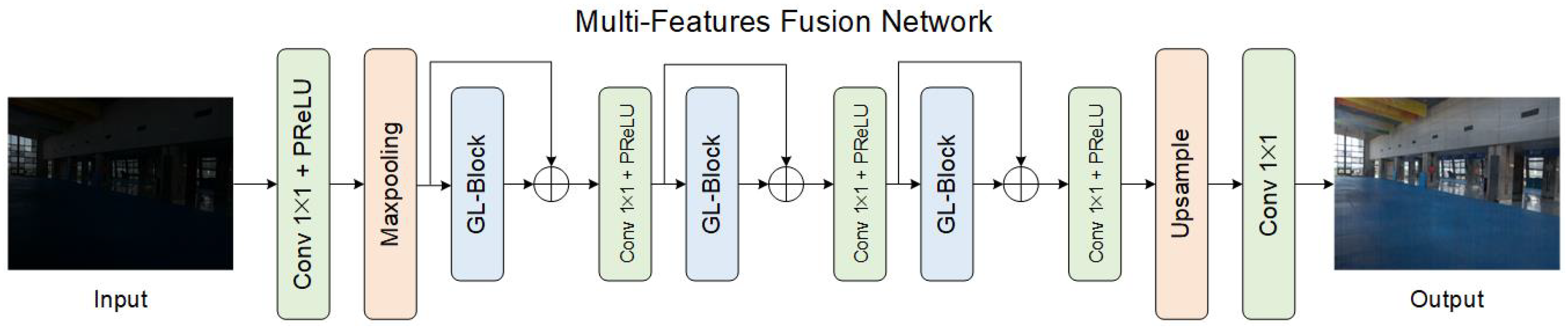
The overview of the network is presented in Figure 2. To reduce the computational complexity, we use $1\times 1$ convolutional and max-pooling layers to downsample the low-visibility image. For feature extraction, we propose the GL-Block consisting of convolutional layers and cross attention modules. In the end, $1\times 1$ convolutional and bilinear upsampling layers transform the output image to the corresponding fine scale.

3.2. GL-Block

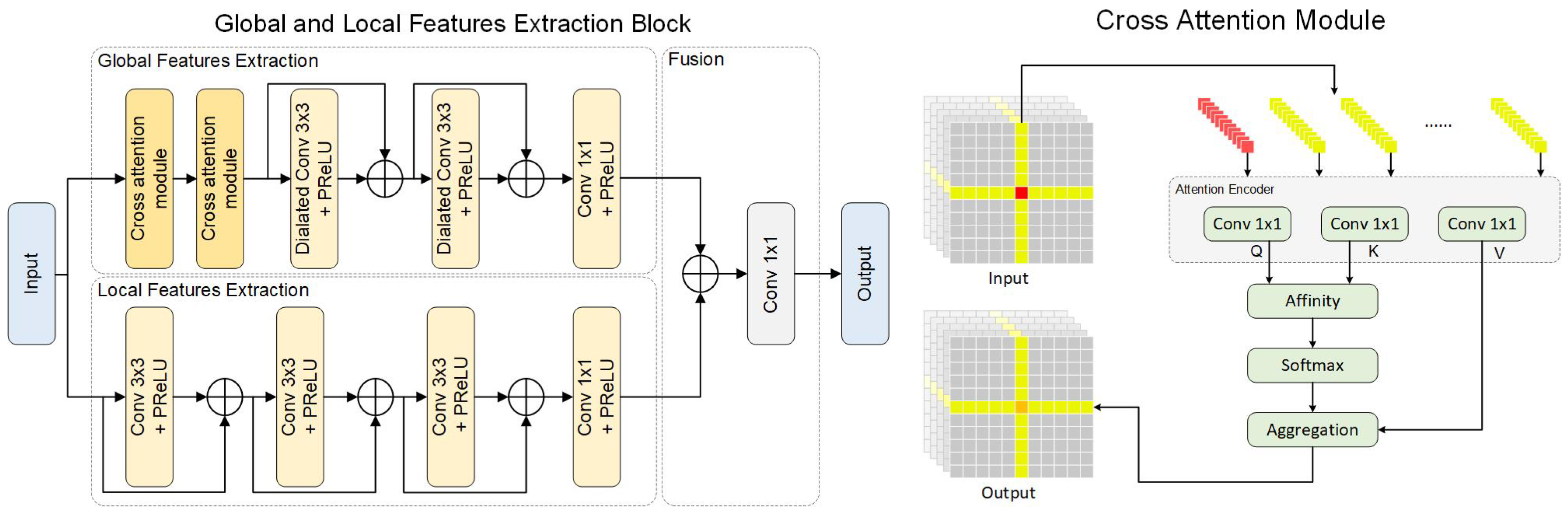
We design a two-branched block to extract multiple features simultaneously. Firstly we employ cross attention modules [23] to extract global features, which collect global information in the horizontal and vertical directions to enhances the representative capability of each pixel, as shown in Figure 3. Specifically, $1\times 1$ convolutional layers are used to obtain the query (Q), key (K), and value (V) matrix and generate the attention map M with an affinity operation. Unlike the common attention method, GL-Block achieves global spatial information interaction with two cross attention modules, which sufficiently reduces the computational complexity. The contextual information collected by the cross attention module can be expressed as

$$M_{i,j}=f(M_{i,j}^{{}^{\prime }},M_{i,\_}^{{}^{\prime }},M_{\_,j}^{{}^{\prime }}),$$

(2)

where $M{{}^{\prime }}_{i,j}$ represents each vector in the input feature maps, $M_{i,\_}^{{}^{\prime }}$ and $M_{\_,j}^{{}^{\prime }}$ represent the horizontal and vertical vectors, respectively, and f denotes the process of establishing the connection between each pixel. However, the cross attention mechanism will cause a black-line problem due to the extremely dark or bright pixels, as discussed in Section 4.6. Therefore, to balance the extreme non-uniformity, we optimize the cross attention module with two subsequent dilated convolutional layers. The kernel size is set to three, and the dilation steps are set to four and six, respectively.

The other branch consists of several residual convolutional layers, designed to extract local features separately. In particular, inspired by [47], the convolutional layers are densely connected for better detail preservation. The kernel size and stride of convolutional layers are set to three and one, respectively. In the end, we merge the global and local feature maps and feed it into a $1\times 1$ convolutional layer for feature fusion.

3.3. Loss Function

For the back-propagation process, we propose a joint loss function consisting of L1 loss ${\mathcal{L}}_1$, L2 loss ${\mathcal{L}}_2$, and color similarity loss ${\mathcal{L}}_{color}$ to supervise our network from both the Euclidean and angle difference. This can be defined as

$$\mathcal{L}={\lambda }_1{\mathcal{L}}_1+{\lambda }_2{\mathcal{L}}_2+{\lambda }_3{\mathcal{L}}_{color},$$

(3)

where ${\lambda }_1$, ${\lambda }_2$, and ${\lambda }_3$ are the weights of each loss function.

L1 Loss. To ensure the quality of the generated images, we employ the widely used L1 loss function, which is based on the Euclidean distance between each pixel. It can be expressed as

$${\mathcal{L}}_1=\frac{1}{hwc}\sum _{i,k}∥P_i^k-{\widehat{P}}_i^k∥,$$

(4)

where $P_i^k$ and ${\widehat{P}}_i^k$ are the pixels of the output images and ground truth, respectively. i and k represent the positions and channels, respectively. h, w, and c denote the height, width and the number of channels, respectively.

L2 Loss. Besides L1, the L2 loss function is also widely used in low-level computer vision tasks for the effective restriction on the output image, which can be expressed as

$${\mathcal{L}}_2=\frac{1}{hwc}\sum _{i,k}{\parallel P_i^k-{\widehat{P}}_i^k\parallel }_2.$$

(5)

Color Similarity Loss. In RGB images, the Euclidean distance is a typical evaluation metrics to validate the similarity between two pixels, However, it ignores the angle difference between two RGB vectors, which also causes severe color differences between two pixels. To measure the deviation more comprehensively, we employ the cosine similarity between each vector as the color similarity loss to take the angle difference into consideration. The color loss function can be expressed as

$${\mathcal{L}}_{color}=1-\frac{1}{hw}·\sum _i\frac{P_i·{\widehat{P}}_i}{max({\parallel P_i\parallel }_2·{\parallel {\widehat{P}}_i\parallel }_2,ϵ)},$$

(6)

where the cosine value of the angle between the RGB vectors $P_i$ and ${\widehat{P}}_i$ is calculated, which represents the angle differences of the pixel at the position i. $ϵ$ = 0.001 is a hyper-parameter used to avoid zero becoming the denominator.

4. Experiments

In this section, we firstly describe the dataset and the implementation details used in the experiment. To comprehensively evaluate the performance of the MFF-Net, different aspects of the state-of-the-art methods and our model are compared including GT reference, noise reduction, color naturalness, and computational complexity. The ablation studies concerning the necessity of multiple feature fusion and the weight settings of the joint loss function are presented to demonstrate the rationality of the proposed method. Finally, to verify the practical benefits of the proposed method, we construct the vessel detection experiments on the enhanced images.

4.1. Dataset and Evaluation Indicators

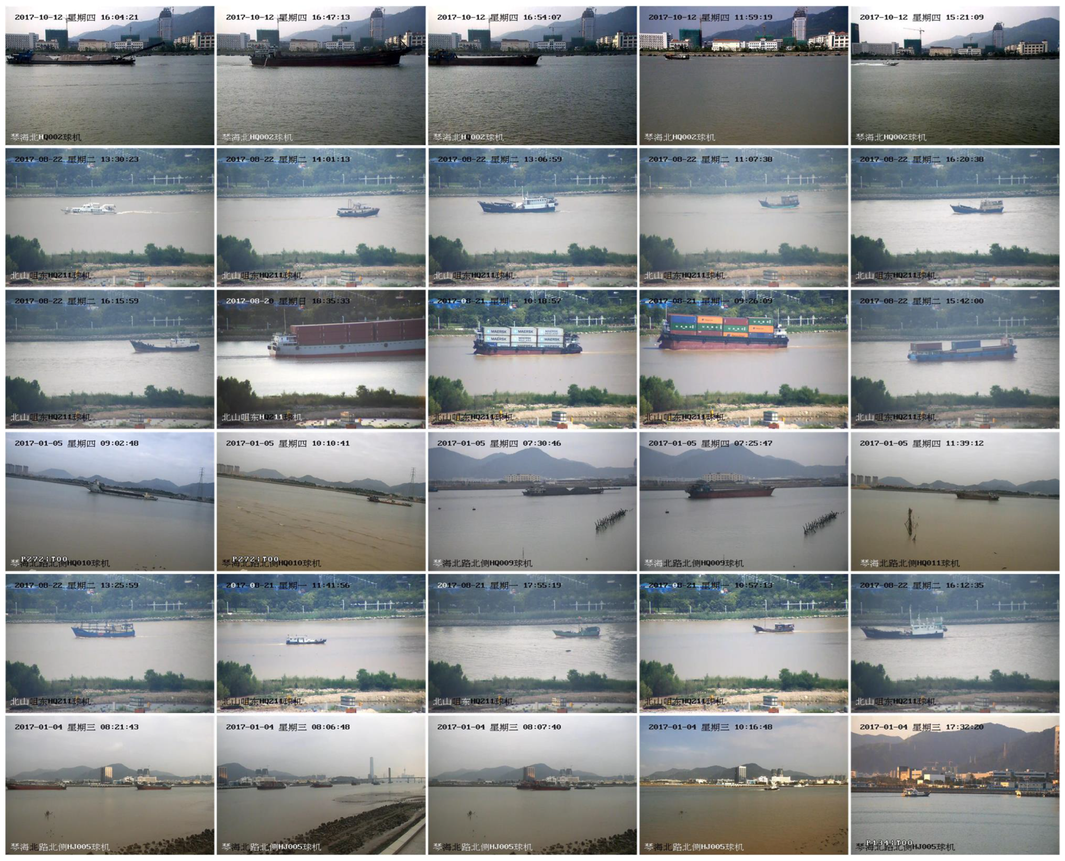
Supervised learning requires the perfectly paired dataset to calculate the pixel difference between the output and ground truth. However, the current publicly available paired datasets (LOL [48], EnlightenGAN [49], I-HAZE [50], SMOKE [51], etc.) are not suitable for maritime low-visbility image enhancement1, and the paired maritime low-visibility image dataset is difficult to obtain. We thus synthesize a large number of marine low-visibility images based on the Seaships dataset. Specifically, we select 1500 high-quality images from the Seaships dataset for training and 30 images for testing, as shown in Figure 4. It is noted that the characters in the image are the timestamps and locations of the camera, which is contained in the original dataset. In low-light image enhancement tasks, we also adopt traditional methods to synthesize low-light maritime images, which can be expressed as

$$L_{\mathrm{maritime}}\left(x\right)=J\left(x\right)\times g\left(x\right),$$

(7)

where $L_{\mathrm{maritime}}\left(x\right)$ is the low-light maritime image, $J\left(x\right)$ is the clear image, and $g\left(x\right)$ is the coefficient, which is a random number between 0.1 and 0.8. Meanwhile, we exploit Equation (1) to obtain synthetic training hazy data. We restrict $t\left(x\right)$ from 0.1 to 0.7, and set A from 0.2 to 0.8. For the test data, we synthesized three types of low-light images with different light levels, i.e., $g_1\left(x\right)$ = 0.2, $g_2\left(x\right)$ = 0.4, and $g_3\left(x\right)$ = 0.6 (termed Test-L). Similarly, we also synthesized three types of images using Equation (1) with different degrees of degradation, i.e., $t_1=0.4/A_1=0.9$, $t_2=0.2/A_2=0.8$, and $t_3=0.2/A_3=0.7$ (termed Test-H).

For the supervised neural network, the results closer to the ground truth represent a better performance. Therefore, for quantitative image quality assessment comparisons, we choose five reference evaluation indicators, i.e., peak signal-to-noise ratio (PSNR), structural similarity (SSIM) [52], feature similarity index measure (FSIM) [53], and visual saliency-induced index (VSI) [54] to evaluate the enhancement performance. It is noted that a higher PSNR, SSIM, FSIM, VSI represent better image quality and a closer proximity to the ground truth.

Figure 4. Thirty selected maritime images from the Seaships [55] dataset, which contains raw maritime surveillance data captured in different scenes.

Figure 4. Thirty selected maritime images from the Seaships [55] dataset, which contains raw maritime surveillance data captured in different scenes.

4.2. Implementation Details

We use Pytorch to build and train the MFF-Net. The network is trained for 300 epochs, and the ADAM optimizer is employed during training. The starting learning rate is set to $1\times {10}^{-3}$ and is multiplied by 0.1 after every 100 epochs. In the loss function, to equally employ the Euclidean distance and the angle difference as the restraint, the weights of ${\mathcal{L}}_1$, ${\mathcal{L}}_2$, and ${\mathcal{L}}_{color}$ are set to 0.25, 0.25, and 0.5, respectively. For data augmentation, we randomly crop the $600\times 400$ images to patches of size 128 × 128 for training and the original size for testing, and the running time costs are calculated on a laptop with an AMD Ryzen 7 5800H CPU accelerated by an NVIDIA GTX 3060 GPU. For a fair comparison, the parameters of all competing methods are from the open access checkpoints by the authors.

4.3. Experiments on Maritime Low-Light Images

To verify the superior performance of our method, we select some competitive classical algorithms and state-of-the-art methods to compare: (a) traditional mathematical model methods, including HE [17], NPE [30], BCP [56], SRIE [57], and LIME [31]; (b) deep learning-based methods, including RetinexNet [48], LightenNet [58], MBLLEN [59], KinD [35], Zero [36], and StableLLVE [18]. The visual comparisons on Test-L are shown in Figure 5. In terms of mathematical model-based methods, the results of HE and BCP have obvious color distortion, some non-uniform artifact exists in the results enhanced by NPE, and LIME fails to lighten the low-light images effectively. In addition, for deep learning-based methods, RetinexNet suffers from severe color distortion, KinD only enhances the image with local features, which is incompatible with the illumination diversity between the non-adjacent patches, Zero sacrifices the enhancement effect for fast speed, making the results look a little dark, and StableLLVE fails to enlighten the extremely dark regions. Compared with these methods, our results look more natural with better recovery. As shown in

Table 2. Quantitative comparison between our method and the state-of-the-art methods on the 90 maritime low-light images. The top three results are marked in red, blue, and green colors, respectively. The ↑ represents that the higher value means better result.

Methods	PSNR ↑	SSIM ↑	FSIM ↑	VSI ↑
HE [17]	18.011 ± 1.838	0.770 ± 0.073	0.896 ± 0.031	0.961 ± 0.013
NPE [30]	21.839 ± 2.936	0.946 ± 0.023	0.977 ± 0.008	0.992 ± 0.003
BCP [56]	16.577 ± 1.857	0.844 ± 0.051	0.929 ± 0.026	0.969 ± 0.016
SRIE [57]	18.044 ± 4.432	0.889 ± 0.074	0.946 ± 0.034	0.986 ± 0.008
LIME [31]	20.597 ± 3.719	0.945 ± 0.026	0.981 ± 0.008	0.993 ± 0.004
RetinexNet [48]	14.927 ± 1.927	0.691 ± 0.093	0.815 ± 0.049	0.943 ± 0.019
LightenNet [58]	11.985 ± 2.702	0.788 ± 0.072	0.916 ± 0.028	0.972 ± 0.008
MBLLEN [59]	13.721 ± 3.065	0.739 ± 0.064	0.950 ± 0.011	0.984 ± 0.004
KinD [35]	17.037 ± 1.413	0.906 ± 0.031	0.954 ± 0.015	0.984 ± 0.009
Zero [36]	17.074 ± 1.421	0.838 ± 0.036	0.891 ± 0.029	0.964 ± 0.017
StableLLVE [18]	14.853 ± 2.921	0.797 ± 0.044	0.898 ± 0.042	0.974 ± 0.011
MFF-Net	23.666 ± 4.222	0.941 ± 0.024	0.978 ± 0.009	0.994 ± 0.003

, the quantitative experiment result indicates that our method achieves a competitive performance on the whole. Although not the best in terms of certain metrics, our proposed method has substantial advantages in running speed, as discussed in Section 4.5.

4.4. Experiments on Maritime Hazy Images

To demonstrate the dehazing ability of MFF-Net, we also select some classical traditional enhancement methods, including DCP [40], CAP [41], HL [60], F-LDCP [61], and GRM [62], and some state-of-the-art learning-based methods, including DehazeNet [42], MSCNN [63], AOD-Net [64], GCANet [44], HTDNet [65], and FFANet [45], for testing. As shown in Figure 6, the image dehazed by DCP suffers serious noise interference, especially on the water surface. Meanwhile, color distortion occurs in some areas. CAP and F-LDCP fail to dehaze the images thoroughly, resulting in the overall image being covered by a layer of haze. In contrast, HL dehazes the images better, but the enhanced image is too bright with serious noise interference. Furthermore, on the edge of the vessel and some of the water surface, the reflection phenomenon seriously influences the visual feeling, which brings a barrier to the lookout. On the whole, the learning-based methods achieve better performance than the traditional methods. However, DehazeNet, MSCNN, and AOD-Net still cannot dehaze the images thoroughly. Furthermore, although GCANet and FFA-Net can remove most of the haze, the images are still riddled with artifacts. The quantitative results are shown in

Table 3. Quantitative comparison between our method and the state-of-the-art methods on the 90 maritime hazy images. The top three results are marked in red, blue, and green colors, respectively. The ↑ represents that the higher value means better result.

Methods	PSNR ↑	SSIM ↑	FSIM ↑	VSI ↑
DCP [15]	15.687 ± 2.437	0.823 ± 0.059	0.946 ± 0.019	0.976 ± 0.011
CAP [41]	19.218 ± 4.078	0.848 ± 0.089	0.906 ± 0.057	0.978 ± 0.013
HL [60]	21.440 ± 2.353	0.917 ± 0.027	0.962 ± 0.019	0.980 ± 0.013
F-LDCP [61]	12.318 ± 1.454	0.645 ± 0.099	0.781 ± 0.077	0.948 ± 0.020
GRM [62]	20.271 ± 2.236	0.815 ± 0.068	0.888 ± 0.042	0.968 ± 0.013
DehazeNet [42]	13.092 ± 1.456	0.683 ± 0.101	0.808 ± 0.076	0.955 ± 0.019
MSCNN [63]	17.084 ± 2.132	0.843 ± 0.075	0.915 ± 0.048	0.980 ± 0.011
AODNet [64]	17.722 ± 2.661	0.761 ± 0.105	0.819 ± 0.074	0.958 ± 0.020
GCANet [44]	19.437 ± 3.066	0.878 ± 0.043	0.952 ± 0.014	0.981 ± 0.007
FFANet [45]	19.918 ± 4.805	0.858 ± 0.076	0.939 ± 0.031	0.984 ± 0.009
MFF-Net	22.192 ± 2.021	0.912 ± 0.028	0.955 ± 0.013	0.988 ± 0.006

. Compared with other methods, MFF-Net can successfully dehaze the images with a good balance between color restoration and detail preservation, benefiting from the strong learning ability of the CNN and the multi-feature fusion strategy. The expoeriments on the real captued images are shown in Figure 7. It can be seen that our method is effective for both real-captured low-light and hazy images.

4.5. Computational Complexity Analysis

In the practical maritime surveillance, the visual enhancement methods must take the running time into account. To evaluate the performance on computational complexity, we provide the running time cost on both low-light image enhancement and dehazing. For low-light enhancement, as shown in

Table 4. Average running time cost (unit: seconds) and parameter comparison on low-light images with different resolutions (400 × 600, 480 × 640, and 768 × 1024) of the different methods.

Methods	Platform	Parameters (K)	400 × 600	480 × 640	768 × 1024
HE [17]	Matlab (CPU)	-	0.1089	0.1344	0.3234
NPE [30]	Matlab (CPU)	-	4.6228	5.7649	14.705
BCP [56]	Matlab (CPU)	-	0.7711	0.9936	2.2191
SRIE [57]	Matlab (CPU)	-	5.1873	8.8056	20.323
LIME [31]	Matlab (CPU)	-	8.2369	11.429	46.887
RetinexNet [48]	Python (GPU)	8536.7	0.0714	0.0922	0.2070
LightenNet [58]	Matlab (GPU)	-	0.0570	0.0640	0.2093
MBLLEN [59]	Python (GPU)	450.2	0.0870	0.1045	0.2493
KinD [35]	Python (GPU)	8017.1	0.1040	0.1469	0.2225
Zero [36]	Python (GPU)	79.4	0.0165	0.0178	0.0315
StableLLVE [18]	Python (GPU)	4316.3	0.1045	0.1501	0.1953
MFF-Net	Python (GPU)	817.3	0.0457	0.0566	0.1657

, MFF-Net is able to enhance the 400 × 600 images at over 20 FPS with the acceleration of an NVIDIA RTX 3060 GPU, which is faster than most other methods. LightenNet [58] and Zero [36] are more lightweight, but the enhancement effect is much worse than ours. For the dehazing method, as shown in

Table 5. Average running time cost (unit: seconds) and the parameters comparison on hazy images with different resolutions (400 × 600, 480 × 640, and 768 × 1024) of the different methods.

Methods	Platform	Parameters (K)	400 × 600	480 × 640	768 × 1024
DCP [40]	Matlab (CPU)	-	0.8124	1.0282	2.8398
CAP [41]	Matlab (CPU)	-	1.1568	1.3286	2.6762
HL [60]	Matlab (CPU)	-	4.9637	5.1852	6.6912
F-LDCP [61]	Matlab (CPU)	-	1.2865	1.4799	3.5562
DehazeNet [42]	Matlab (GPU)	-	0.5243	0.6742	1.4918
MSCNN [63]	Matlab (GPU)	-	0.1965	0.2853	0.8973
AODNet [64]	Python (GPU)	9	0.0125	0.0141	0.0192
GCANet [44]	Python (GPU)	2758	0.0912	0.1055	0.1722
FFANet [45]	Python (GPU)	25,999	0.7236	0.7951	1.8978
MFF-Net	Python (GPU)	817.3	0.0457	0.0566	0.1657

, our MFF-Net also outperforms most of the previous methods. AOD-Net is faster, but the effectiveness of dehazing is worse than ours. In general, MFF-Net achieves a superior balance between the enhancement effect and the running time cost compared with the other methods, as depicted in Figure 8.

4.6. Ablation Study

To validate the necessity of multiple feature fusion guidance, we first conduct the ablation experiment on the architecture with two incomplete versions: (a) with only the local feature guidance network (OLF-Net), which only employs the dense connected convolutional layers to extract the local features during the processing; and (b) with only the global feature guidance network (OGF-Net), which only uses the optimized cross attention module to extract global features. The visual results are shown in Figure 9, the enhanced image of OLF-Net suffers from obvious dark artifacts, which proves that the shallow convolutional layers cannot meet the learning capabilities required for extremely low-visibility image enhancement tasks. In addition, the noticeable black-line issue exists in the OGF-Net, due to the effect of exceptionally dark or bright pixels on correlated pixels in the cross attention module. The ablation study on the architecture indicates that multiple feature fusion guidance successfully improves the effectiveness of feature representation and alleviates the excessive influence of extremely bright or dark pixels in the cross attention mechanism, which is necessary in low-visibility enhancement tasks.

We also investigate the effectiveness of the weight setting on different loss functions, including the Euclidean distance (${\mathcal{L}}_1+{\mathcal{L}}_2$) and angle difference (${\mathcal{L}}_{color}$). For a fair experiment, the architecture of the network is set to MFF-Net. According to the comparison of the quantitative indicators shown in

Table 6. Quantitative quality assessment comparison between different weight distributions of the loss functions on the testing data consisting of paired images extracted from the LOL [48] and EnlightenGAN [49] datasets. ↑ and ↓ represent that higher or lower values mean the better results, respectively.

Loss Functions	PSNR↑	SSIM↑	LPIPS↓
0.25${\mathcal{L}}_1+0.25{\mathcal{L}}_2$	21.34 ± 4.4286	0.760 ± 0.1336	0.151 ± 0.1098
0.25${\mathcal{L}}_1+0.25{\mathcal{L}}_2+0.25{\mathcal{L}}_{color}$	21.30 ± 4.6006	0.763 ± 0.1302	0.148 ± 0.1070
0.125${\mathcal{L}}_1+0.125{\mathcal{L}}_2+0.25{\mathcal{L}}_{color}$	21.40 ± 3.6208	0.753 ± 0.1253	0.170 ± 0.1177
0.25${\mathcal{L}}_1+0.25{\mathcal{L}}_2+0.5{\mathcal{L}}_{color}$	21.36 ± 4.2196	0.779 ± 0.1251	0.139 ± 0.1003

, the network shows the best performance on the proposed weight setting, which guarantee the enhancement quality comprehensively with a rational balance between the Euclidean distance and angle difference.

4.7. Improvement in Maritime Vessel Detection

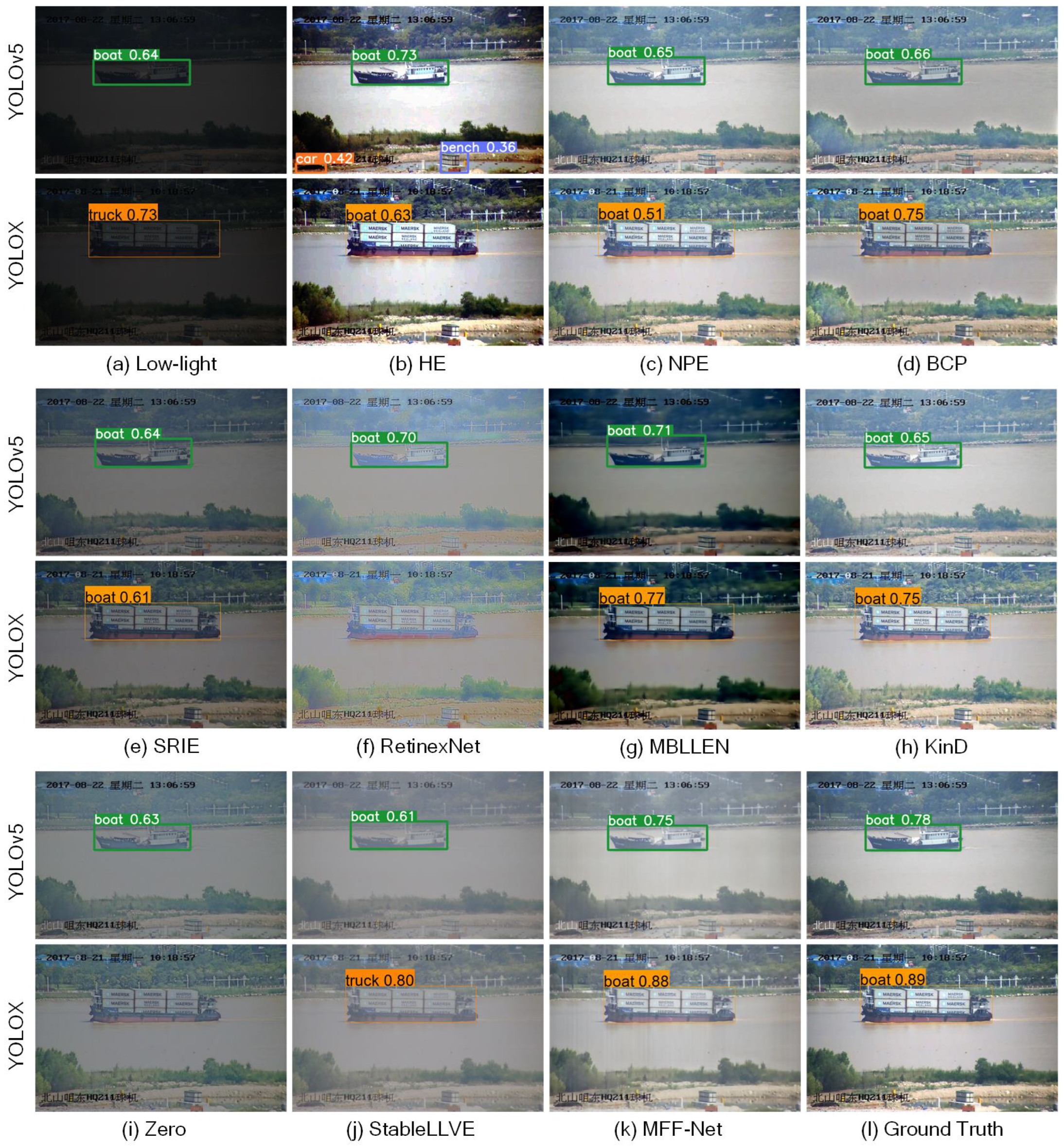
To further demonstrate the practical benefits of our MFF-Net for maritime surveillance under low-visibility weathers, we apply YOLOv5 and YOLOX [68] to conduct maritime vessel detection experiments. The test images are randomly selected from the Test-L and Test-H. First, we select 1500 maritime-related images in the COCO dataset to train our detection networks. The evaluation tests are then constructed on the selected images. In low-visibility scenes, the vessel detection accuracy decreases heavily due to the low contrast and vague edge features, which can cause difficulties in maritime surveillance. In other words, the caption cannot make full use of the computer vision to assist the artificial lookout. After enhancement, the visual data can deliver clearer traffic scenes to the managers, and the detection accuracy is also significantly increased. The experimental results are illustrated in Figure 10 and Figure 11. Compared with the state-of-the-art methods, the enhanced results of the MFF-Net perform better due to the application of multi-feature fusion. The quantitative comparison is shown in

Table 7. Quantitative experiments about the vessel detection accuracy improvement on YOLOX, which is tested on the Seaships [55] dataset. It is noted that mAP (clear), mAP (low-visibility), and mAP (enhancement) represent the mean average precision on clear, low-visbility, and enhanced images, respectively.

Weather	Method	mAP (Clear)	mAP (Low-Visibility)	mAP (Enhancement)
	HE [17]	40.97%	31.97%	33.26%
Low-light	Zero [36]	40.97%	31.97%	35.11%
	MFF-Net	40.97%	31.97%	36.42%
	DCP [15]	40.97%	21.66%	26.25%
Hazy	AOD-Net [64]	40.97%	21.66%	32.37%
	MFF-Net	40.97%	21.66%	34.81%

. It is noted that the input image will be first resized to 640 × 640 in YOLOX. However, most of the traditional method cannot enhance them within one second; thus, they cannot be applied in practical engineering. Therefore, we compare our method with the fastest representative traditional and deep learning-based methods in a quantitative experiment. The experimental results demonstrate that the MFF-Net has practical benefits in maritime surveillance, which is more beneficial for higher-level visual tasks under low-visibility weathers when assisting artificial observations, thereby improving maritime management.

5. Conclusions

In this paper, we proposed an end-to-end multi-feature fusion-guided low-visbility enhancement method for maritime surveillance. Firstly, the maritime low-visibility images, i.e., low-light and hazy, are downsampled and then fed into the GL-Block comprising cross attention modules and dense residual convolutional layers. The GL-Block is designed to extract the global and local features to guide the enhancement processing simultaneously. After enhancement, the image is upsampled to a finer scale. For better constraint of the enhanced output, we introduced a joint loss function comprising L1 loss, L2 loss, and color similarity loss. In the experiments, we made massive comparisons on the visual performance, including quantitative image quality assessment, noise reduction, and color naturalness on both low-light enhancement and dehazing. Compared with other methods, the MFF-Net achieved a competitive quantitative and visual performance with effective noise reduction and superior color naturalness. Moreover, we evaluated the operating time cost and model size of the state-of-the-art methods, which indicates that MFF-Net can efficiently enhance extremely low-visibility images with lower computational complexity. In the ablation study, we conducted a series of experiments to investigate the necessity of multiple feature guidance and rational weight settings of the proposed loss function. Finally, the experiment of vessel detection indicate that our method is beneficial for practical maritime surveillance under low-visibility weathers.

In the future, we will test more methods for global feature extraction to demonstrate the advantages of multiple features for low-visibility image enhancement. Furthermore, high-definition videos cannot currently be enhanced in real time. We will thus optimize the architecture of the MFF-Net to achieve a better performance with lower computational complexity, which will enable the network to work on a diverse range of maritime edge devices.

References

- Zhang, M.; Kujala, P.; Musharraf, M.; Zhang, J.; Hirdaris, S. A machine learning method for the prediction of ship motion trajectories in real operational conditions. Ocean Eng. 2023, 283, 114905. [Google Scholar] [CrossRef]
- Zhang, M.; Taimuri, G.; Zhang, J.; Hirdaris, S. A deep learning method for the prediction of 6-DoF ship motions in real conditions. Proc. Inst. Mech. Eng. Part J. Eng. Marit. Environ. 2023. [Google Scholar] [CrossRef]
- Guo, Y.; Liu, R.W.; Qu, J.; Lu, Y.; Zhu, F.; Lv, Y. Asynchronous Trajectory Matching-Based Multimodal Maritime Data Fusion for Vessel Traffic Surveillance in Inland Waterways. IEEE Trans. Intell. Transp. Syst. 2023; to be published. [Google Scholar] [CrossRef]
- Qu, J.; Liu, R.W.; Guo, Y.; Lu, Y.; Su, J.; Li, P. Improving maritime traffic surveillance in inland waterways using the robust fusion of AIS and visual data. Ocean Eng. 2023, 275, 114198. [Google Scholar] [CrossRef]
- Yang, W.; Wang, S.; Fang, Y.; Wang, Y.; Liu, J. From fidelity to perceptual quality: A semi-supervised approach for low-light image enhancement. In Proceedings of the IEEE/CVF Conference on Computer Vision and Pattern Recognition, Virtual, 13–19 June 2020; pp. 3063–3072. [Google Scholar]
- Liu, Y.L.; Lai, W.S.; Chen, Y.S.; Kao, Y.L.; Yang, M.H.; Chuang, Y.Y.; Huang, J.B. Single-image HDR reconstruction by learning to reverse the camera pipeline. In Proceedings of the IEEE/CVF Conference on Computer Vision and Pattern Recognition, Virtual, 14–19 June 2020; pp. 1651–1660. [Google Scholar]
- Liu, D.; Wen, B.; Jiao, J.; Liu, X.; Wang, Z.; Huang, T.S. Connecting image denoising and high-level vision tasks via deep learning. IEEE Trans. Image Process. 2020, 29, 3695–3706. [Google Scholar] [CrossRef] [PubMed]
- Zhou, Z.; Zhao, J.; Chen, X.; Chen, Y. A Ship Tracking and Speed Extraction Framework in Hazy Weather Based on Deep Learning. J. Mar. Sci. Eng. 2023, 11, 1353. [Google Scholar] [CrossRef]
- Guo, Y.; Lu, Y.; Liu, R.W. Lightweight deep network-enabled real-time low-visibility enhancement for promoting vessel detection in maritime video surveillance. J. Navig. 2021, 75, 230–250. [Google Scholar] [CrossRef]
- Ma, R.; Bao, K.; Yin, Y. Improved Ship Object Detection in Low-Illumination Environments Using RetinaMFANet. J. Mar. Sci. Eng. 2022, 10, 1996. [Google Scholar] [CrossRef]
- Fan, Y.; Niu, L.; Liu, T. Multi-Branch Gated Fusion Network: A Method That Provides Higher-Quality Images for the USV Perception System in Maritime Hazy Condition. J. Mar. Sci. Eng. 2022, 10, 1839. [Google Scholar] [CrossRef]
- Wang, H.; Chen, Y.; Cai, Y.; Chen, L.; Li, Y.; Sotelo, M.A.; Li, Z. SFNet-N: An Improved SFNet Algorithm for Semantic Segmentation of Low-Light Autonomous Driving Road Scenes. IEEE Trans. Intell. Transp. Syst. 2022, 23, 21405–21417. [Google Scholar] [CrossRef]
- Liu, R.W.; Guo, Y.; Lu, Y.; Chui, K.T.; Gupta, B.B. Deep network-enabled haze visibility enhancement for visual IoT-driven intelligent transportation systems. IEEE Trans. Industr. Inform. 2022, 19, 1581–1591. [Google Scholar] [CrossRef]
- Qu, J.; Gao, Y.; Lu, Y.; Xu, W.; Liu, R.W. Deep learning-driven surveillance quality enhancement for maritime management promotion under low-visibility weathers. Ocean Coast. Manag. 2023, 235, 106478. [Google Scholar] [CrossRef]
- Krishnan, D.; Fergus, R. Dark flash photography. ACM Trans. Graph. 2009, 28, 96. [Google Scholar] [CrossRef]
- Lu, Y.; Jung, S.W. Progressive Joint Low-Light Enhancement and Noise Removal for Raw Images. IEEE Trans. Image Process. 2022, 31, 2390–2404. [Google Scholar] [CrossRef]
- Abdullah-Al-Wadud, M.; Kabir, M.H.; Dewan, M.A.A.; Chae, O. A dynamic histogram equalization for image contrast enhancement. IEEE Trans. Consum. Electron. 2007, 53, 593–600. [Google Scholar] [CrossRef]
- Zhang, S.; Lam, E.Y. Learning to restore light fields under low-light imaging. Neurocomputing 2021, 456, 76–87. [Google Scholar] [CrossRef]
- Liu, M.; Tang, L.; Zhong, S.; Luo, H.; Peng, J. Learning noise-decoupled affine models for extreme low-light image enhancement. Neurocomputing 2021, 448, 21–29. [Google Scholar] [CrossRef]
- Qin, J.; Zhang, R. Lightweight Single Image Super-Resolution with Attentive Residual Refinement Network. Neurocomputing 2022, 500, 846–855. [Google Scholar] [CrossRef]
- Hu, X.; Zhu, L.; Wang, T.; Fu, C.W.; Heng, P.A. Single-image real-time rain removal based on depth-guided non-local features. IEEE Trans. Image Process. 2021, 30, 1759–1770. [Google Scholar] [CrossRef]
- Sun, Z.; Zhang, Y.; Bao, F.; Wang, P.; Yao, X.; Zhang, C. SADnet: Semi-supervised single image dehazing method based on an attention mechanism. ACM Trans. Multimed. Comput. Commun. Appl. 2022, 18, 1–23. [Google Scholar] [CrossRef]
- Huang, Z.; Wang, X.; Huang, L.; Huang, C.; Wei, Y.; Liu, W. Ccnet: Criss-cross attention for semantic segmentation. In Proceedings of the IEEE/CVF International Conference on Computer Vision, Seoul, Republic of Korea, 27 Oceober–2 November 2019; pp. 603–612. [Google Scholar]
- Wang, C.; Fan, B.; Li, Y.; Xiao, J.; Min, L.; Zhang, J.; Chen, J.; Lin, Z.; Su, S.; Wu, R.; et al. Study on the Classification Perception and Visibility Enhancement of Ship Navigation Environments in Foggy Conditions. J. Mar. Sci. Eng. 2023, 11, 1298. [Google Scholar] [CrossRef]
- Huang, S.C.; Cheng, F.C.; Chiu, Y.S. Efficient contrast enhancement using adaptive gamma correction with weighting distribution. IEEE Trans. Image Process. 2012, 22, 1032–1041. [Google Scholar] [CrossRef]
- Jobson, D.J.; Rahman, Z.u.; Woodell, G.A. A multiscale retinex for bridging the gap between color images and the human observation of scenes. IEEE Trans. Image. Process. 1997, 6, 965–976. [Google Scholar] [CrossRef] [PubMed]
- Lee, C.; Lee, C.; Kim, C.S. Contrast enhancement based on layered difference representation. In Proceedings of the 2012 19th IEEE International Conference on Image Processing, Orlando, FL, USA, 30 September–3 October 2012; IEEE: New York, NY, USA, 2012; pp. 965–968. [Google Scholar]
- Lee, C.; Lee, C.; Kim, C.S. Contrast enhancement based on layered difference representation of 2D histograms. IEEE Trans. Image Process. 2013, 22, 5372–5384. [Google Scholar] [CrossRef] [PubMed]
- Jobson, D.J.; Rahman, Z.U.; Woodell, G.A. Properties and performance of a center/surround retinex. IEEE Trans. Image Process. 1997, 6, 451–462. [Google Scholar] [CrossRef]
- Wang, S.; Zheng, J.; Hu, H.M.; Li, B. Naturalness preserved enhancement algorithm for non-uniform illumination images. IEEE Trans. Image Process. 2013, 22, 3538–3548. [Google Scholar] [CrossRef]
- Guo, X.; Li, Y.; Ling, H. LIME: Low-light image enhancement via illumination map estimation. IEEE Trans. Image Process. 2016, 26, 982–993. [Google Scholar] [CrossRef]
- Chen, C.; Chen, Q.; Xu, J.; Koltun, V. Learning to see in the dark. In Proceedings of the IEEE Conference on Computer Vision and Pattern Recognition, Salt Lake City, UT, USA, 18–22 June 2018; pp. 3291–3300. [Google Scholar]
- Wang, K.; Gao, P.; Hoi, S.; Guo, Q.; Qian, Y. Extreme Low-Light Imaging with Multi-granulation Cooperative Networks. arXiv 2020, arXiv:2005.08001. [Google Scholar]
- Lu, Y.; Guo, Y.; Zhu, F.; Liu, R.W. Towards Low-Visibility Enhancement in Maritime Video Surveillance: An Efficient and Effective Multi-Deep Neural Network. In Proceedings of the 2021 IEEE International Intelligent Transportation Systems Conference (ITSC), Indianapolis, IN, USA, 19–22 September 2021; IEEE: New York, NY, USA, 2021; pp. 2869–2874. [Google Scholar]
- Zhang, Y.; Zhang, J.; Guo, X. Kindling the darkness: A practical low-light image enhancer. In Proceedings of the 27th ACM International Conference on Multimedia, Nice, France, 21–25 October 2019; pp. 1632–1640. [Google Scholar]
- Guo, C.; Li, C.; Guo, J.; Loy, C.C.; Hou, J.; Kwong, S.; Cong, R. Zero-reference deep curve estimation for low-light image enhancement. In Proceedings of the IEEE/CVF Conference on Computer Vision and Pattern Recognition, Virtual, 14–19 June 2020; pp. 1780–1789. [Google Scholar]
- Hao, S.; Han, X.; Guo, Y.; Wang, M. Decoupled Low-Light Image Enhancement. ACM Trans. Multimed. Comput. Commun. Appl. 2022, 18, 1–19. [Google Scholar] [CrossRef]
- Guo, Y.; Lu, Y.; Qu, J.; Liu, R.W.; Ren, W. MDSFE: Multiscale Deep Stacking Fusion Enhancer Network for Visual Data Enhancement. IEEE Trans. Instrum. Meas. 2022, 72, 1–12. [Google Scholar] [CrossRef]
- Wang, Y.; Wan, R.; Yang, W.; Li, H.; Chau, L.P.; Kot, A. Low-light image enhancement with normalizing flow. In Proceedings of the AAAI Conference on Artificial Intelligence, Virtual, 22 February–1 March 2022; pp. 2604–2612. [Google Scholar]
- He, K.; Sun, J.; Tang, X. Single image haze removal using dark channel prior. IEEE Trans. Pattern Anal. Mach. Intell. 2010, 33, 2341–2353. [Google Scholar] [PubMed]
- Zhu, Q.; Mai, J.; Shao, L. A fast single image haze removal algorithm using color attenuation prior. IEEE Trans. Image Process. 2015, 24, 3522–3533. [Google Scholar] [PubMed]
- Cai, B.; Xu, X.; Jia, K.; Qing, C.; Tao, D. Dehazenet: An end-to-end system for single image haze removal. IEEE Trans. Image Process. 2016, 25, 5187–5198. [Google Scholar] [CrossRef] [PubMed]
- Tang, G.; Zhao, L.; Jiang, R.; Zhang, X. Single image dehazing via lightweight multi-scale networks. In Proceedings of the 2019 IEEE International Conference on Big Data (Big Data), Los Angeles, CA, USA, 9–12 December 2019; IEEE: New York, NY, USA, 2019; pp. 5062–5069. [Google Scholar]
- Chen, D.; He, M.; Fan, Q.; Liao, J.; Zhang, L.; Hou, D.; Yuan, L.; Hua, G. Gated context aggregation network for image dehazing and deraining. In Proceedings of the IEEE Winter Conference on Applications of Computer Vision, Waikoloa, HI, USA, 7–11 January 2019; IEEE: New York, NY, USA, 2019; pp. 1375–1383. [Google Scholar]
- Qin, X.; Wang, Z.; Bai, Y.; Xie, X.; Jia, H. FFA-Net: Feature fusion attention network for single image dehazing. In Proceedings of the AAAI Conference on Artificial Intelligence, New York, NY, USA, 7–12 February 2020; pp. 11908–11915. [Google Scholar]
- Guo, Y.; Gao, Y.; Liu, W.; Lu, Y.; Qu, J.; He, S.; Ren, W. SCANet: Self-Paced Semi-Curricular Attention Network for Non-Homogeneous Image Dehazing. In Proceedings of the IEEE/CVF Conference on Computer Vision and Pattern Recognition, Vancouver, BC, Canada, 18–22 June 2023; pp. 1884–1893. [Google Scholar]
- Iandola, F.; Moskewicz, M.; Karayev, S.; Girshick, R.; Darrell, T.; Keutzer, K. Densenet: Implementing efficient convnet descriptor pyramids. arXiv 2014, arXiv:1404.1869. [Google Scholar]
- Wei, C.; Wang, W.; Yang, W.; Liu, J. Deep retinex decomposition for low-light enhancement. arXiv 2018, arXiv:1808.04560. [Google Scholar]
- Jiang, Y.; Gong, X.; Liu, D.; Cheng, Y.; Fang, C.; Shen, X.; Yang, J.; Zhou, P.; Wang, Z. Enlightengan: Deep light enhancement without paired supervision. IEEE Trans. Image Process. 2021, 30, 2340–2349. [Google Scholar] [CrossRef]
- Ancuti, C.; Ancuti, C.O.; Timofte, R.; De Vleeschouwer, C. I-HAZE: A dehazing benchmark with real hazy and haze-free indoor images. In Proceedings of the Advanced Concepts for Intelligent Vision Systems: 19th International Conference, ACIVS 2018, Poitiers, France, 24–27 September 2018; Proceedings 19. Springer: Cham, Switzerland, 2018; pp. 620–631. [Google Scholar]
- Jin, Y.; Yan, W.; Yang, W.; Tan, R.T. Structure representation network and uncertainty feedback learning for dense non-uniform fog removal. In Proceedings of the Asian Conference on Computer Vision, Macao, China, 4–8 December 2022; Springer: Cham, Switzerland, 2022; pp. 155–172. [Google Scholar]
- Wang, Z.; Bovik, A.C.; Sheikh, H.R.; Simoncelli, E.P. Image quality assessment: From error visibility to structural similarity. IEEE Trans. Image Process. 2004, 13, 600–612. [Google Scholar] [CrossRef]
- Zhang, L.; Zhang, L.; Mou, X.; Zhang, D. FSIM: A feature similarity index for image quality assessment. IEEE Trans. Image Process. 2011, 20, 2378–2386. [Google Scholar] [CrossRef]
- Zhang, L.; Shen, Y.; Li, H. VSI: A visual saliency-induced index for perceptual image quality assessment. IEEE Trans. Image Process. 2014, 23, 4270–4281. [Google Scholar] [CrossRef]
- Shao, Z.; Wu, W.; Wang, Z.; Du, W.; Li, C. Seaships: A large-scale precisely annotated dataset for ship detection. IEEE Trans. Multimed. 2018, 20, 2593–2604. [Google Scholar] [CrossRef]
- Fu, X.; Zeng, D.; Huang, Y.; Ding, X.; Zhang, X.P. A variational framework for single low light image enhancement using bright channel prior. In Proceedings of the IEEE Global Conference on Signal and Information Processing, Austin, TX, USA, 3–5 December 2013; IEEE: New York, NY, USA, 2013; pp. 1085–1088. [Google Scholar]
- Fu, X.; Zeng, D.; Huang, Y.; Zhang, X.P.; Ding, X. A weighted variational model for simultaneous reflectance and illumination estimation. In Proceedings of the IEEE Conference on Computer Vision and Pattern Recognition (CVPR), Las Vegas, NV, USA, 26 June–1 July 2016; pp. 2782–2790. [Google Scholar]
- Li, C.; Guo, J.; Porikli, F.; Pang, Y. LightenNet: A convolutional neural network for weakly illuminated image enhancement. Pattern Recognit. Lett. 2018, 104, 15–22. [Google Scholar] [CrossRef]
- Lv, F.; Lu, F.; Wu, J.; Lim, C. MBLLEN: Low-Light Image/Video Enhancement Using CNNs. In Proceedings of the BMVC, Newcastle, UK, 3–6 September 2018; p. 220. [Google Scholar]
- Berman, D.; Treibitz, T.; Avidan, S. Air-light estimation using haze-lines. In Proceedings of the 2017 IEEE International Conference on Computational Photography (ICCP), Stanford, CA, USA, 12–14 May 2017; IEEE: New York, NY, USA, 2017; pp. 1–9. [Google Scholar]
- Zhu, Y.; Tang, G.; Zhang, X.; Jiang, J.; Tian, Q. Haze removal method for natural restoration of images with sky. Neurocomputing 2018, 275, 499–510. [Google Scholar] [CrossRef]
- Chen, C.; Do, M.N.; Wang, J. Robust image and video dehazing with visual artifact suppression via gradient residual minimization. In Proceedings of the European Conference on Computer Vision, Amsterdam, The Netherlands, 11–14 October 2016; Springer: Cham, Switzerland, 2016; pp. 576–591. [Google Scholar]
- Ren, W.; Liu, S.; Zhang, H.; Pan, J.; Cao, X.; Yang, M.H. Single image dehazing via multi-scale convolutional neural networks. In Proceedings of the European Conference on Computer Vision, Amsterdam, The Netherlands, 11–14 October 2016; Springer: Cham, Switzerland, 2016; pp. 154–169. [Google Scholar]
- Li, B.; Peng, X.; Wang, Z.; Xu, J.; Feng, D. Aod-net: All-in-one dehazing network. In Proceedings of the IEEE International Conference on Computer Vision, Venice, Italy, 22–29 October 2017; pp. 4770–4778. [Google Scholar]
- Guo, Y.; Lu, Y.; Liu, R.W.; Wang, L.; Zhu, F. Heterogeneous Twin Dehazing Network for Visibility Enhancement in Maritime Video Surveillance. In Proceedings of the 2021 IEEE International Intelligent Transportation Systems Conference (ITSC), Indianapolis, IN, USA, 19–22 September 2021; IEEE: New York, NY, USA, 2021; pp. 2875–2880. [Google Scholar]
- Vonikakis, V.; Bouzos, O.; Andreadis, I. Multi-exposure image fusion based on illumination estimation. In Proceedings of the Signal and Image Processing and Applications SIPA 2011, Crete, Greece, 22–24 June 2011; pp. 135–142. [Google Scholar]
- Prasad, D.K.; Rajan, D.; Rachmawati, L.; Rajabally, E.; Quek, C. Video processing from electro-optical sensors for object detection and tracking in a maritime environment: A survey. IEEE Trans. Intell. Transp. Syst. 2017, 18, 1993–2016. [Google Scholar] [CrossRef]
- Ge, Z.; Liu, S.; Wang, F.; Li, Z.; Sun, J. Yolox: Exceeding yolo series in 2021. arXiv 2021, arXiv:2107.08430. [Google Scholar]
Figure 1.
Examples of the comparison between maritime low-visibility images and clear images.
Figure 2.
Flowchart of the proposed MFF-Net. Firstly, the low-visibility image is downsampled with a max-pooling layer. The multiple features are then extracted with three GL-Blocks to guide the enhancement process. The enhanced image is finally upsampled to the original scale.
Figure 3.
The detailed implementation of the GL-Block and cross attention module.
Figure 5.
Visual comparison of the synthetic low-light images from the Seaships [55] dataset with other competitive methods: (a) low-light; (b) HE [17]; (c) NPE [30]; (d) BCP [56]; (e) SRIE [57]; (f) LIME [31]; (g) RetinexNet [48]; (h) LightenNet [58]; (i) MBLLEN [59]; (j) KinD [35]; (k) Zero [36]; (l) StableLLVE [18]; (m) MFF-Net; (n) ground truth.
Figure 6.
Visual comparison on the synthetic hazy image from the Seaships [55] dataset with other competitive methods: (a) hazy; (b) DCP [40]; (c) CAP [41]; (d) HL [60]; (e) F-LDCP [61]; (f) GRM [62]; (g) DehazeNet [42]; (h) MSCNN [63]; (i) AODNet [64]; (j) GCANet [44]; (k) HTDNet [65]; (l) FFANet [45]; (m) MFF-Net; (n) ground truth.
Figure 7.
Visual performance on the physically captured low-visibility images. The first row contains the low-light images extracted from the TMDIED [66] dataset, and the third row contains the hazy images extracted from SMD [67] and online websites. The corresponding enhanced results of our MFF-Net are shown in the second and fourth rows.
Figure 8.
The trade-off between the visibility enhancement performance and the computational efficiency on several state-of-the-art low-light enhancement and dehazing methods. It is noted that the frame per second (FPS) metric is tested on a 600 × 400 resolution image.
Figure 9.
Visual comparison between the enhanced results of the MFF-Net with the incomplete versions on the standard low-light image enhancement dataset. It is noted that the results in the ablation study are output from the network trained and tested with the same implementation details as the MFF-Net.
Figure 10.
Vessel detection experiment results on maritime low-light images between our method and other competitive methods: (a) low-light; (b) HE [17]; (c) NPE [30]; (d) BCP [56]; (e) SRIE [57]; (f) RetinexNet [48]; (g) MBLLEN [59]; (h) KinD [35]; (i) Zero [36]; (j) StableLLVE [18]; (k) MFF-Net; (l) ground truth. It can be seen that our MFF-Net significantly improves the accuracy of vessel detection under low-light environments, which demonstrates the benefits of our MFF-Net for practical ocean engineering.
Figure 11.
Vessel detection experiment results on maritime hazy images between our method and other competitive methods: (a) hazy; (b) DCP [40]; (c) CAP [41]; (d) HL [60]; (e) F-LDCP [61]; (f) MSCNN [63]; (g) AODNet [64]; (h) GCANet [44]; (i) DehazeNet [42]; (j) FFANet [45]; (k) MFF-Net; (l) ground truth. It can be seen that our MFF-Net significantly improves the accuracy of vessel detection under hazy environments, which demonstrates the benefits of our MFF-Net for practical ocean engineering.