Article

Deep-Water Dynamics along the 2012–2020 Observations on the Continental Margin of the Southern Adriatic Sea (Mediterranean Sea)

by
Francesco Paladini de Mendoza
1,2,
Katrin Schroeder
1,*,
Leonardo Langone
3,
Jacopo Chiggiato
1,
Mireno Borghini
4,
Patrizia Giordano
3 and
Stefano Miserocchi
3
1
Consiglio Nazionale delle Ricerche-Istituto di Scienze Marine (CNR-ISMAR), Arsenale Tesa 104, Castello 2737/F, 30122 Venezia, Italy
2
Consiglio Nazionale delle Ricerche-Istituto di Scienze Polari (CNR-ISP), Via S. Raineri 86, 98122 Messina, Italy
3
Consiglio Nazionale delle Ricerche-Istituto di Scienze Polari (CNR-ISP), Via P. Gobetti 101, 40129 Bologna, Italy
4
Consiglio Nazionale delle Ricerche-Istituto di Scienze Marine (CNR-ISMAR), Forte Santa Teresa, Pozzuolo di Lerici, 19036 La Spezia, Italy
*
Author to whom correspondence should be addressed.
J. Mar. Sci. Eng. 2023, 11(7), 1364; https://doi.org/10.3390/jmse11071364
Submission received: 4 May 2023 / Revised: 26 June 2023 / Accepted: 30 June 2023 / Published: 4 July 2023
(This article belongs to the Section Physical Oceanography)

Abstract

:
This work presents the results of long-term deep-water observations carried out in the southwestern Adriatic margin. Hydrodynamics and thermohaline measurements were carried out in the last 100 m of the water column using two long-term moorings placed at two different locations along the western sector of the Adriatic continental margin (open slope vs. submarine canyon). The observations, carried out over a period of almost 10 years, made it possible to define the intra- and interannual deep-water dynamics, which are mainly influenced by the passage of cold, dense water. The hydrodynamic field is influenced by seasonal behavior and varies from year to year, with no clear temporal trend or periodicity. Thermohaline properties follow hydrodynamics but also show a climatological trend toward higher temperatures and salinity. The combination and variability of preconditioning factors explains the interannual variability in dense water passage at the mooring sites triggering the formation of dense water in the northern Adriatic. The impulsive nature of the dense water flow, which is difficult to capture with sporadic oceanographic surveys, and its linkage with the large-scale atmospheric circulation make continuous monitoring essential to answer open questions about cascading processes and deep-water dynamics under a global change scenario.

1. Introduction

The Adriatic Sea is a sub-basin of the eastern Mediterranean Sea connected to the Ionian Sea by the Strait of Otranto. It is oriented SE–NW and has a length of 800 km and an average width of 180 km. The northern and central parts of the Adriatic basin are generally characterized by shallow waters. However, there is a shelf edge in the southern sector, where the basin reaches the maximum depth of 1200 m in the Southern Adriatic Pit (SAP). In the southern sector lies the continental margin, formed during the last half million years as a result of eustatic depositional cycles and complex Quaternary uplift and deformation patterns [1,2]. In the western sector, the continental margin (see Figure 1b) is characterized by a complex system of depositional and erosional features that testify to strong bottom-current activity [3,4,5,6,7,8]. The Bari Canyon System (hereafter BCS), extending southward from the Gargano promontory, characterizes the continental margin with two main branches. Its total length is about 30 km in a west–east direction [7,9,10] and it is about 10 km wide. The Adriatic Sea is considered one of the hotspots for dense water (DW) production in the Mediterranean Sea [11]. Their formation is not limited to this area but occurs in several places worldwide, as summarized by Ivanov [12]. Their formation is related to meteorological forcings, the dynamics of which varies from place to place but leads to an increase in the density of surface water sinking into the deep layers. In particular, the North Adriatic Dense Water (NAdDW) is a dense shelf water that forms mainly in winter during intense cold outbreaks [11,13,14]. In any case, the formation and dynamics of the DW are fundamental for the recent morphological processes of the continental slope [7,15], carbon sequestration, ventilation, and particle transport in the deep layers [9,16,17]. After its formation, the NAdDW spreads southward along the Italian coast, driven by Coriolis and gravitational forces [18,19,20]. The spreading process, which is also controlled by tides and waves [21], pushes the water masses to the edge of the shelf, where the DW masses can cascade along the southern Adriatic slope, and can seasonally affect the entire western Adriatic margin [7]. The Adriatic Sea is the main source of bottom water and DW of the eastern Mediterranean, and the first studies on the dynamics of the NAdDW started many years ago [22,23]. Since the reassessment of the dynamics of the Adriatic Sea by Orlic et al. [24], numerous studies have focused on the dynamics, formation, circulation pathways, and related processes of the NAdDW [25,26,27]. Since 2013, glider observations have been conducted twice a year in winter in the SAP along the Bari–Dubrovnik transect to monitor the dynamics of the DW [28]. Since 2006, the South Adriatic trench observatory named E2M3A “http://nettuno.ogs.trieste.it/e2-m3a/”(accessed on 29 June 2023) has been located in the center of the cyclonic gyre in the southern Adriatic basin, where deep convection processes occur. This observatory, which represents the longest nearly continuous offshore time series available in the region [29], consists of a surface buoy and a secondary mooring line with sensors at different depths for physical and chemical measurements of seawater properties in the surface and bottom layers [30,31,32,33,34,35,36]. In 2012, a large experiment, called Operation Dense Water, was conducted after two weeks of severe cold in the southern Adriatic Sea to observe the dynamics of DW masses [37]. These activities provide a unique multidisciplinary overview of DW dynamics and related processes, ranging from oceanographic modeling to physical and biogeochemical oceanographic observations to sedimentology and geomorphology. The moorings were strategically placed in the southern Adriatic basin, specifically in the open furrow area of the continental slopes and the main channel of the BCS in the western sector of the continental margin.
By their localization, the datasets are representative of two different dynamic conditions, as DW flows along the continental slope of the southern basin have different characteristics.
Monitoring continued at the two sites from 2012, resulting in the collection of long-term data. The moorings are equipped with an ADCP-RDI system and CTD probes that measure currents in the last 100 m of the water column and thermohaline properties. The two moorings, together with the E2M3A observatory [38], are part of the IFON network (Italian Fixed-Point Observatory Network) [39] and the European Multidisciplinary Seafloor and water column Observatory European Research Infrastructure Consortium (EMSO-ERIC) regional facility for the southern Adriatic Sea “http://emso.eu/observatories-node/south-adriatic-sea/” (accessed on 29 June 2023). The full dataset is freely available at “https://doi.org/10.5281/zenodo.6770201” (accessed on 29 June 2023) [40] and represents one of the longest continuous observatories of the Mediterranean Sea.
Previous works in the study area [3,17,41,42,43,44,45] are mainly limited to the 2012 cascading event and leave some questions unanswered. One of the most important questions concerns the recurrence of the DW cascading over time and the variability in DW mass properties.
Long-term records along the southern Adriatic margin make an important contribution to the observation of oceanographic processes in the Adriatic Sea and complement the long-term observations carried out in the northern sector [46] along the west–east transect from Italy to Croatia and in the central Adriatic along the Palagruža Sill transect [47,48,49,50]. The time series of moorings can provide a synoptic observation from the formation of DWs in the northern basin to their passage along the continental margin in the southern Adriatic. The records may be useful in linking the preconditioning factors for DW formation to the dynamics of the observed cascading phenomenon along the continental slope.
In this work, observations over a period of almost 10 years were used to define the presence of seasonal and climatological trends in the dynamics of the near-bottom water column along the continental margin of the Adriatic Sea with an emphasis on cascading phenomena. The dynamics of the DW cascading flow at the mooring sites is also related to the preconditioning factors in the northern Adriatic basin. The role of preconditioning factors has previously been demonstrated by modelling experiments and observations focused on single events [42,51,52]. In this work, direct observations of cascading associated with preconditioning factors are extended to a broad time interval. As in other locations around the globe, DW formation and dynamics are regulated by a complex air–land–sea interaction that has direct implications for biogeochemical cycles and trophic networks that are focal points in the context of climate change. Continuous monitoring in this area thus provides a unique observatory for studying deep-sea dynamic processes and their changes over time.

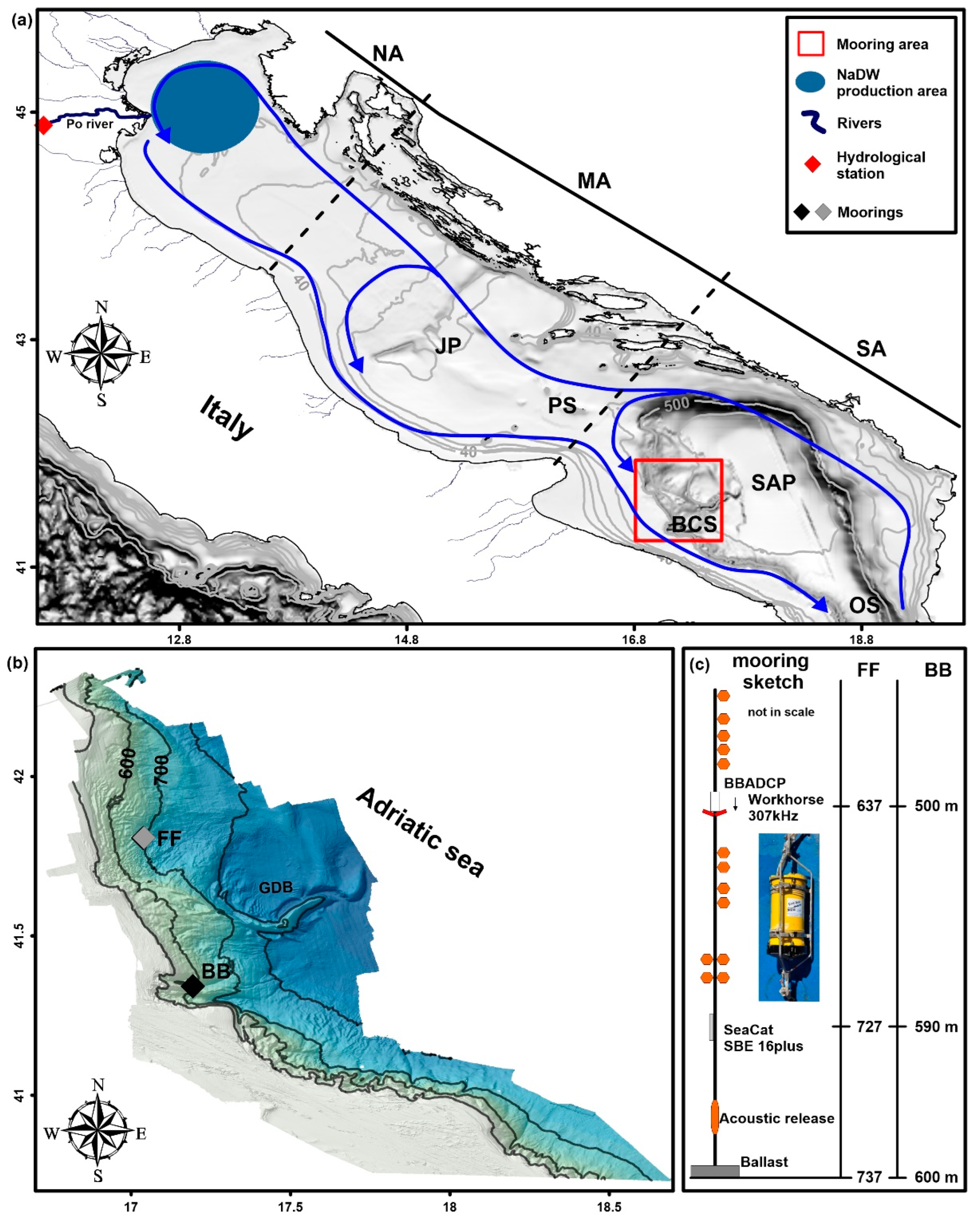
2. Setting, Instruments, Data, and Methods
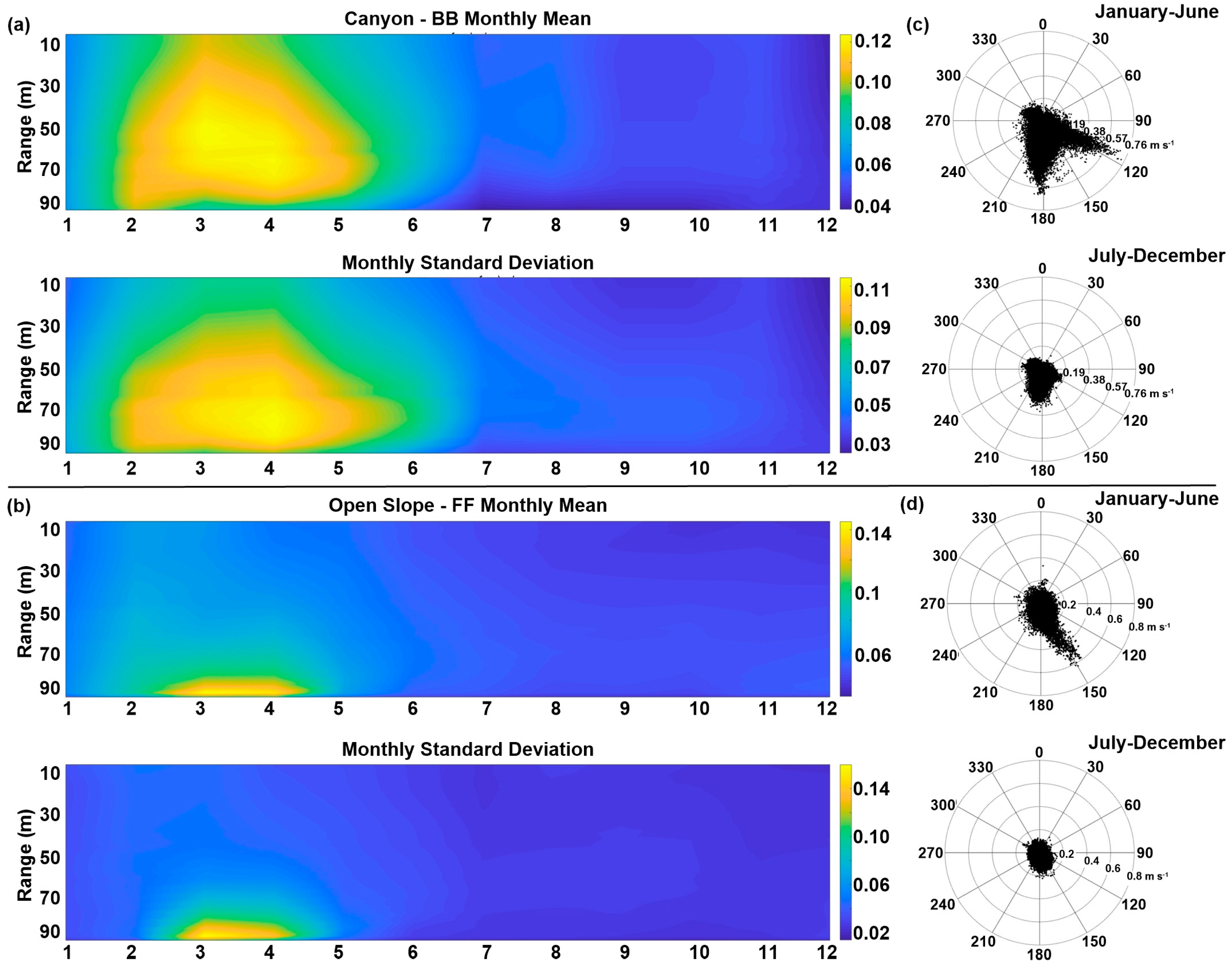
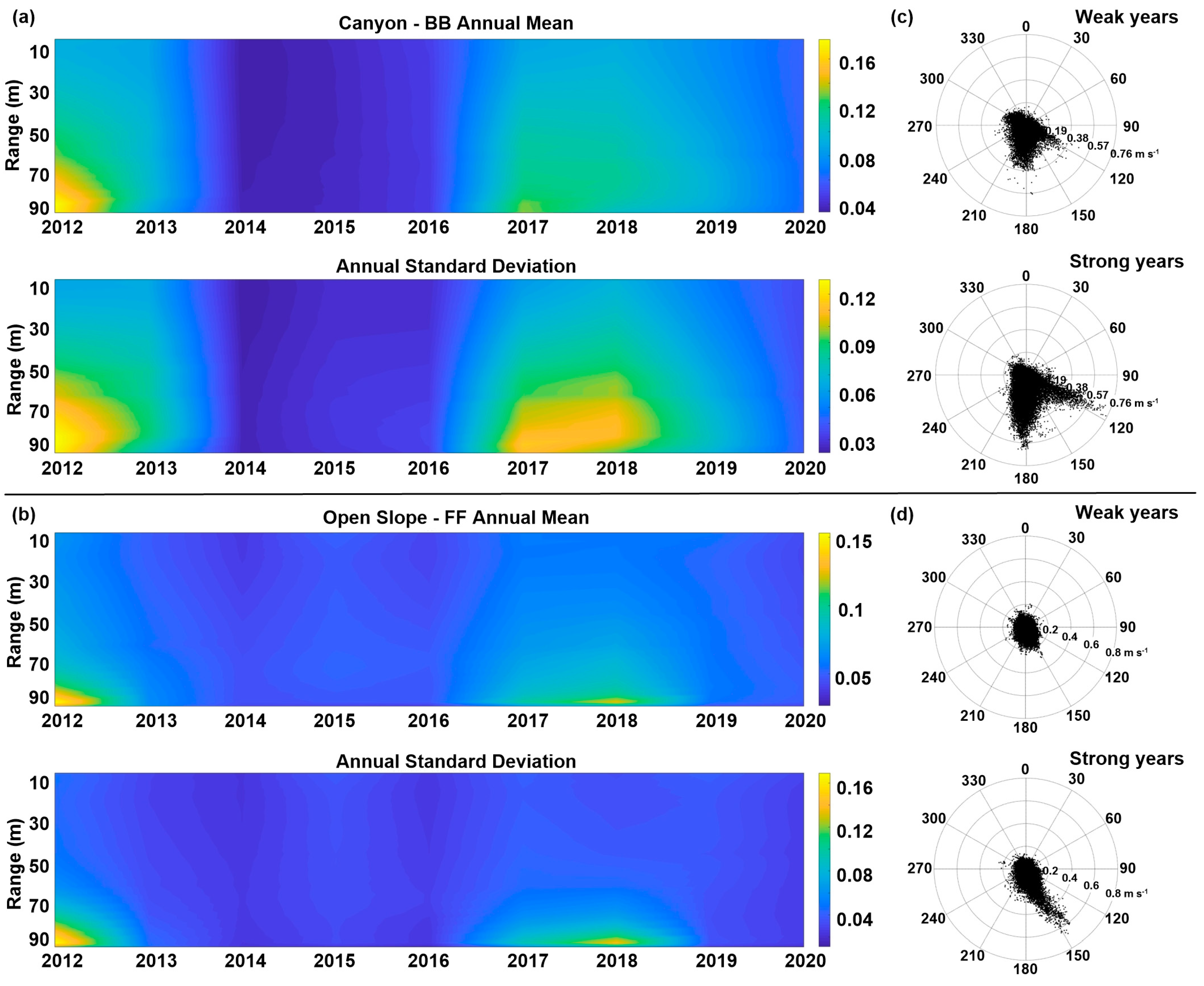
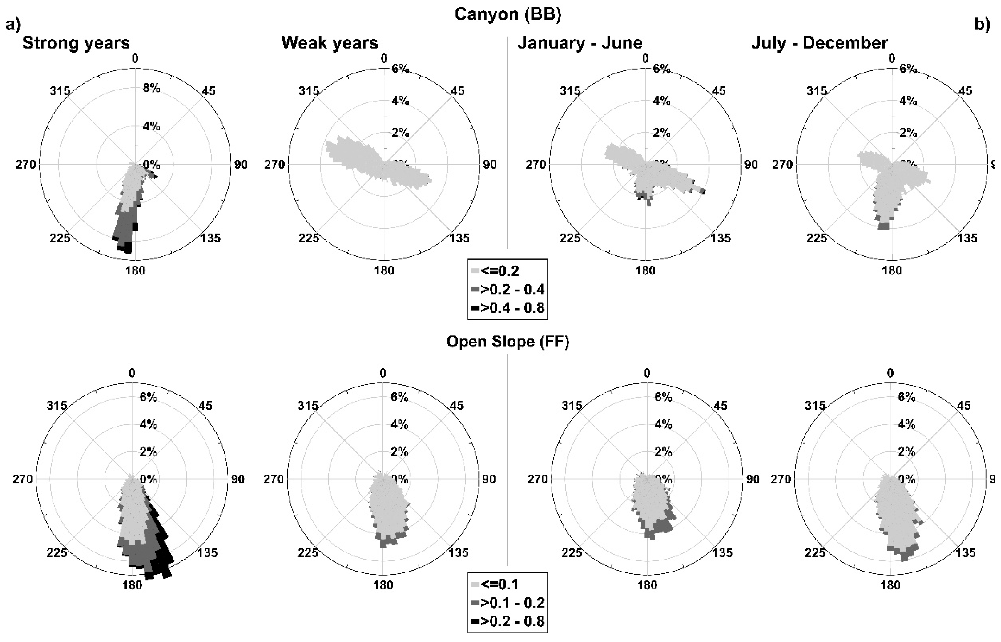
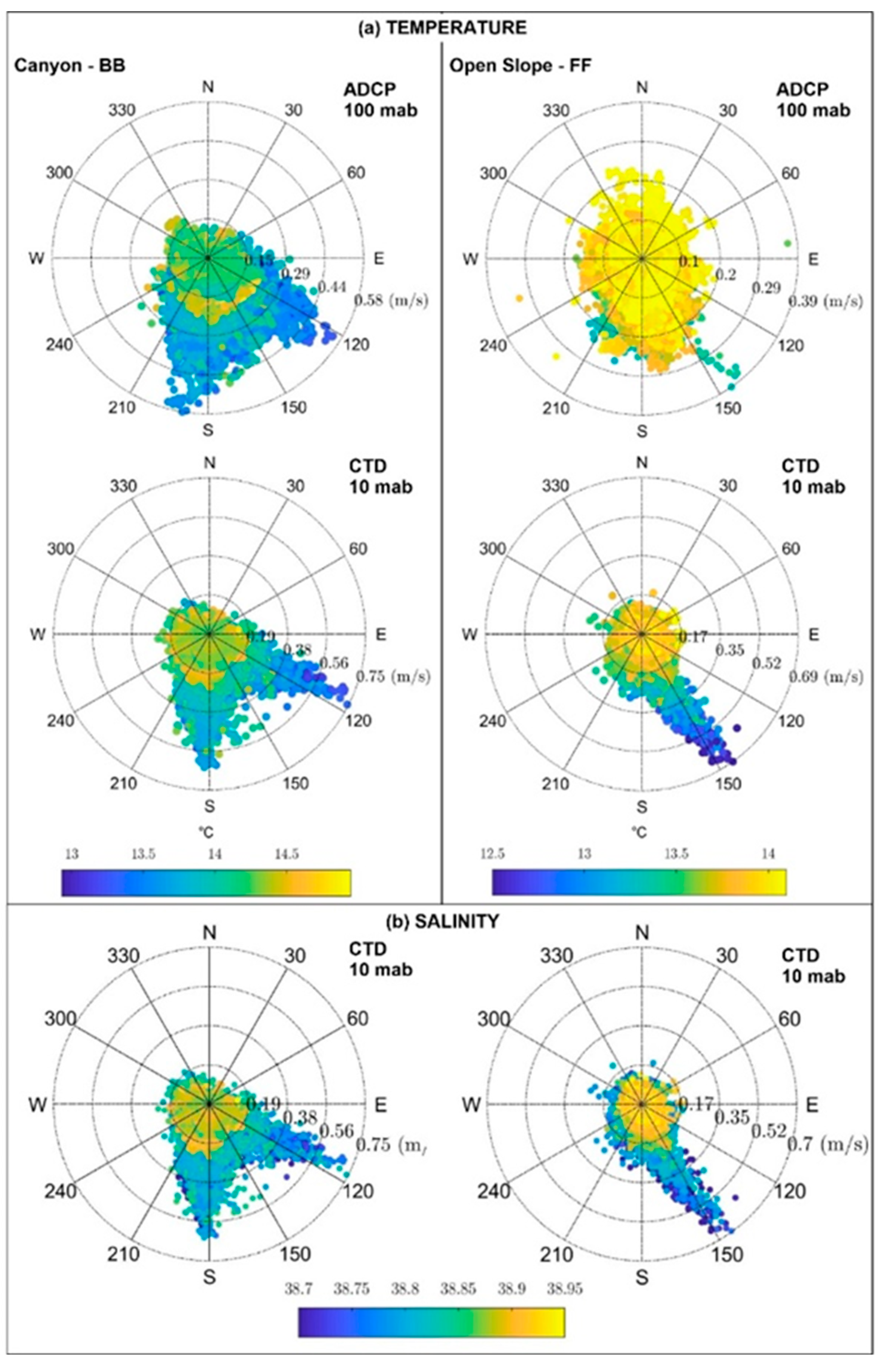
Data were recorded with CTD (Conductivity, Temperature, Depth) and ADCP (Acoustic Doppler Current Profiler) instruments attached to two 110 m moorings along the edge of the southern Adriatic Sea (Figure 1). The two moorings are located at depths of 600 m (BB) and 700 m (FF) on the main branch of the BCS (at 41°20.456′ N and 17°11.639′ E) and in an area of open slope (at 41°48.396′ N and 17°02.217′ E), respectively. The ADCP used is a 300 kHz RDI Workhorse (Teledyne RD Instruments USA, Poway, CA, USA) equipped with a temperature sensor on the transducer head that is mounted facing downward approximately 100 m above the seafloor. The system records currents every 30 min. Detailed information on the system can be found in Paladini de Mendoza et al. [51].
The Seabird self-recording CTD (SBE 16plus V2 SeaCAT) is mounted about 10 m above the seafloor and measures thermohaline parameters every 30 min. Nearly continuous deployments at six-month intervals cover the 2012–2020 time window. All temporal extents of the individual measurements are listed in Table 1 of Paladini de Mendoza et al. [53]. For site BB, records of thermohaline data measured by the CTD at 10 m above the seabed from 2010 to 2012, during the activities presented in Langone et al. [17], were added to the 2012–2020 time series. By extending the time series on a decadal scale, the presence of a climatological trend could be assessed as described in Section 3.1. The maintenance operations, instrument details, calibrations, deployment configurations, data processing methods, and quality control procedures during the measurement period are described in detail in Section 2 of the same document [53]. The water mass properties used to identify DW are analyzed using the T-S diagram, which is also used to observe the relationships between the variations in thermohaline properties and hydrodynamics. The T-S diagram was created with the Gibbs SeaWater (GSW) Oceanographic Toolbox [54] using the TEOS-10 equation “https://www.teos-10.org/index.htm” (accessed on 29 June 2023) to determine the conservative temperature and absolute salinity calculated from in situ CTD measurements of temperature, pressure, and practical salinity.

3. Results

This section presents the inter- and intra-annual characteristics of the thermohaline and hydrodynamic parameters recorded by the measurement systems installed at the moorings to observe the presence of seasonal and climatological trends.

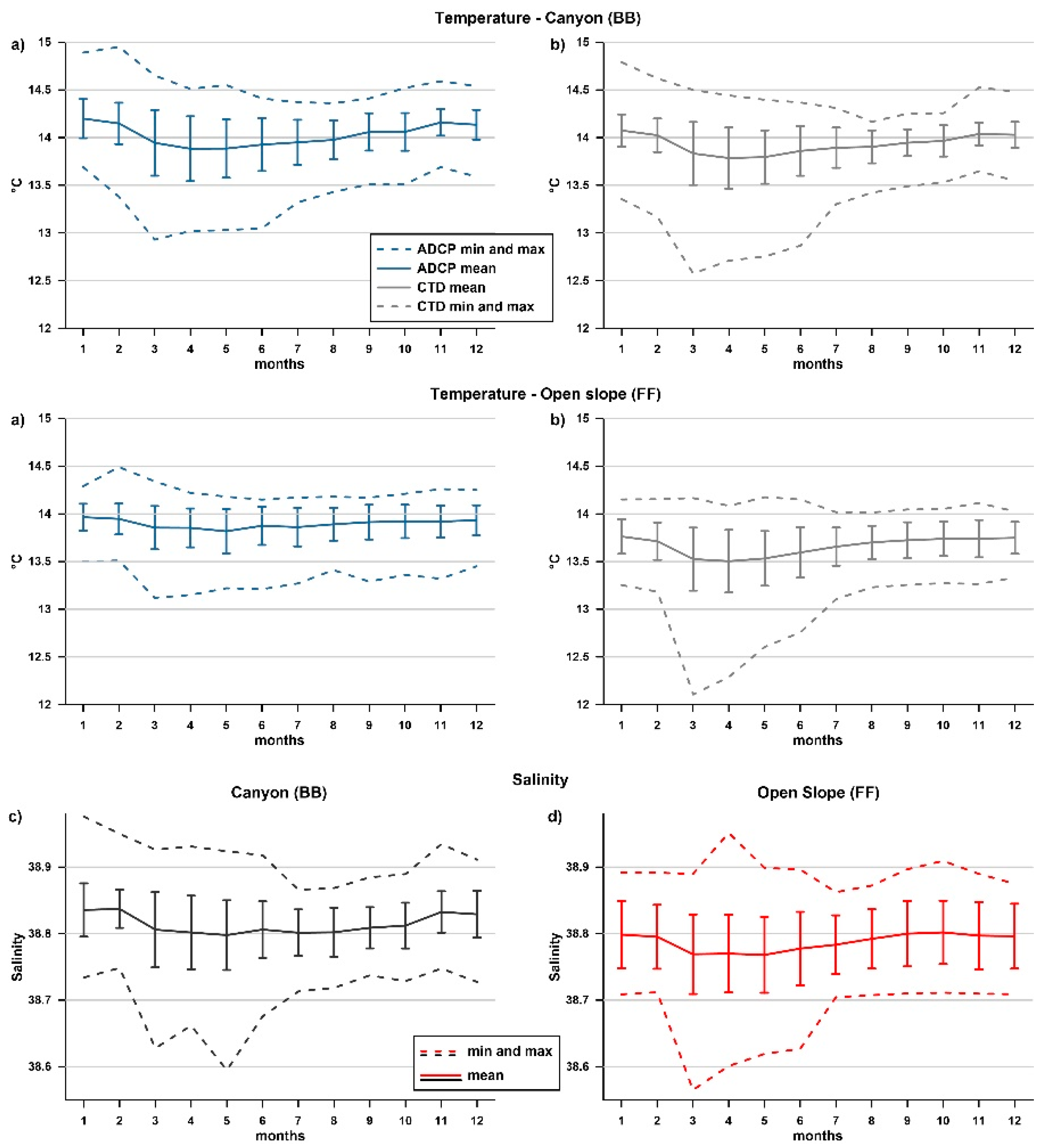
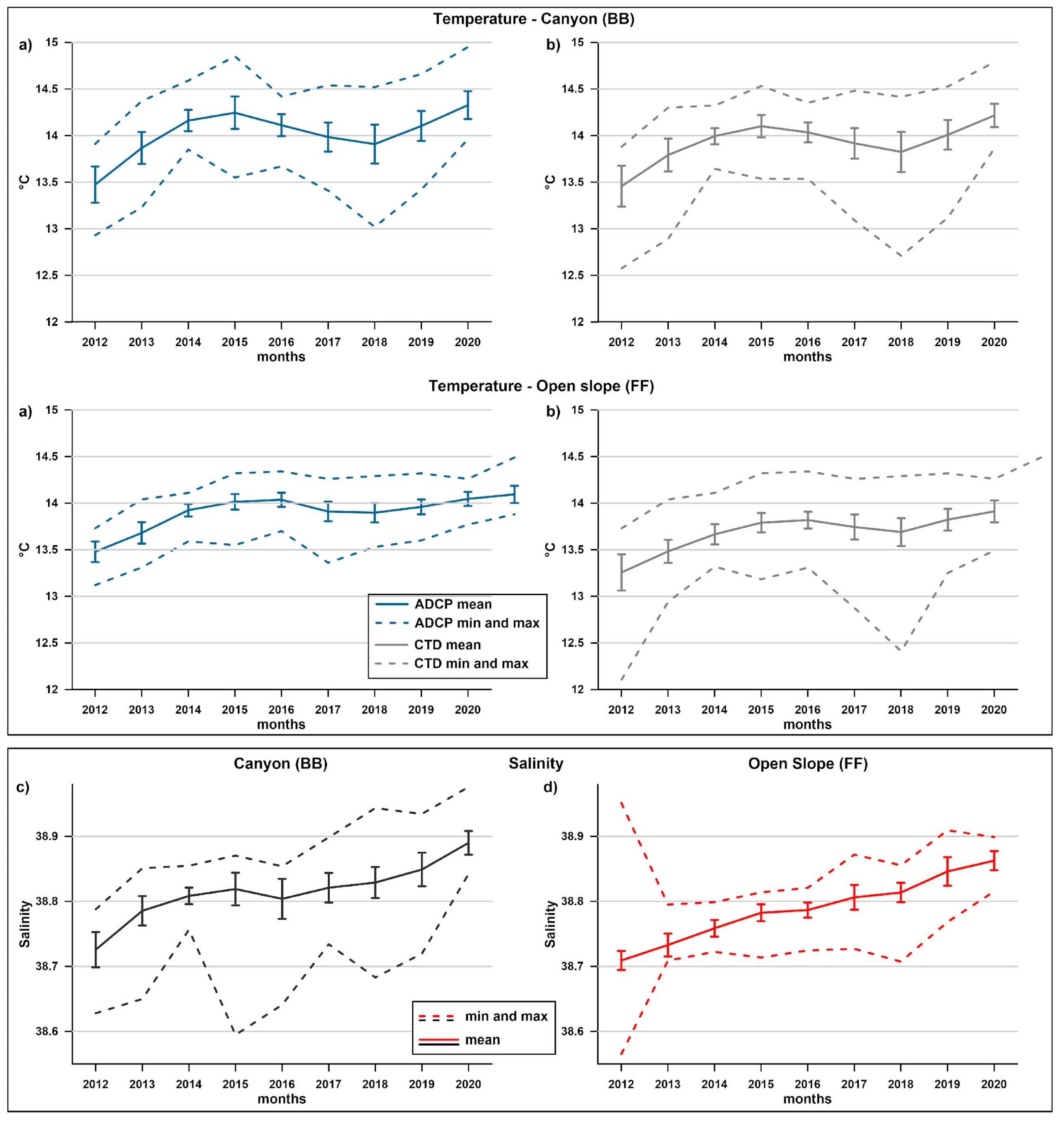
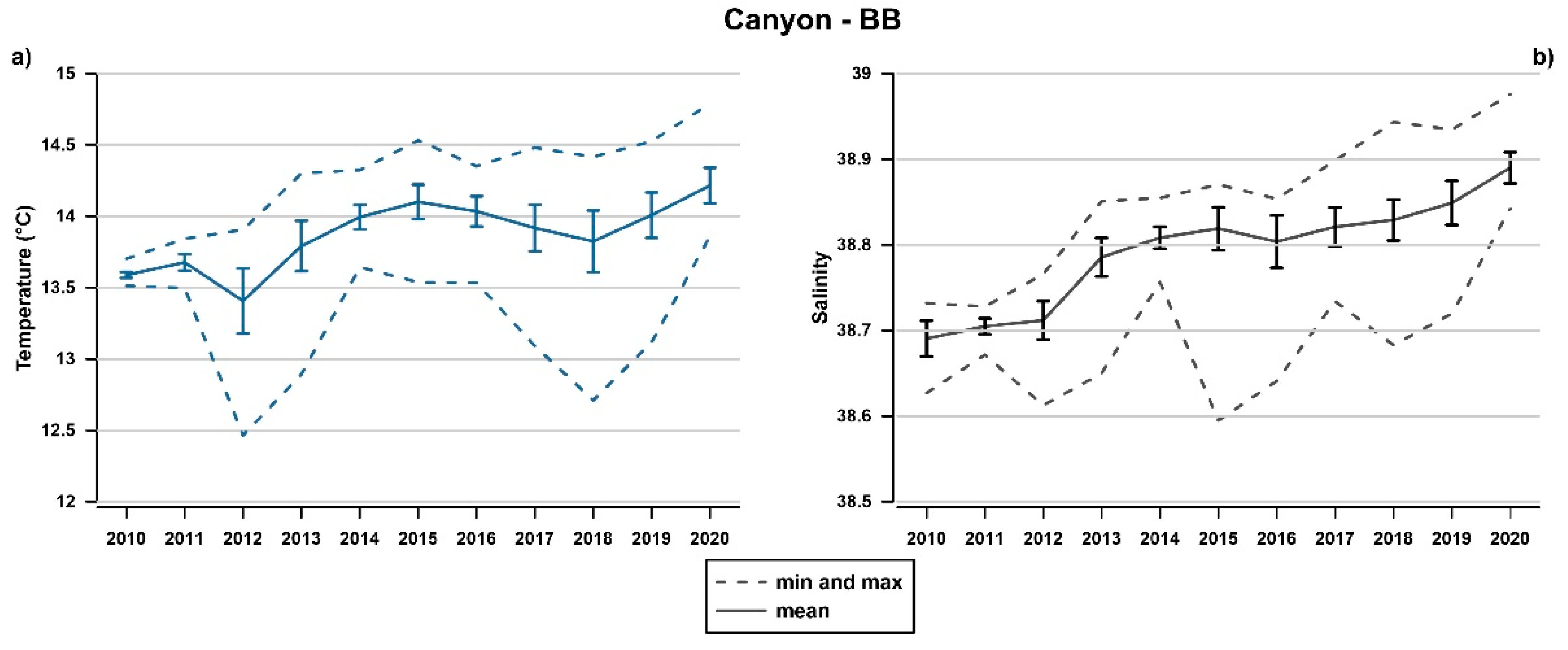
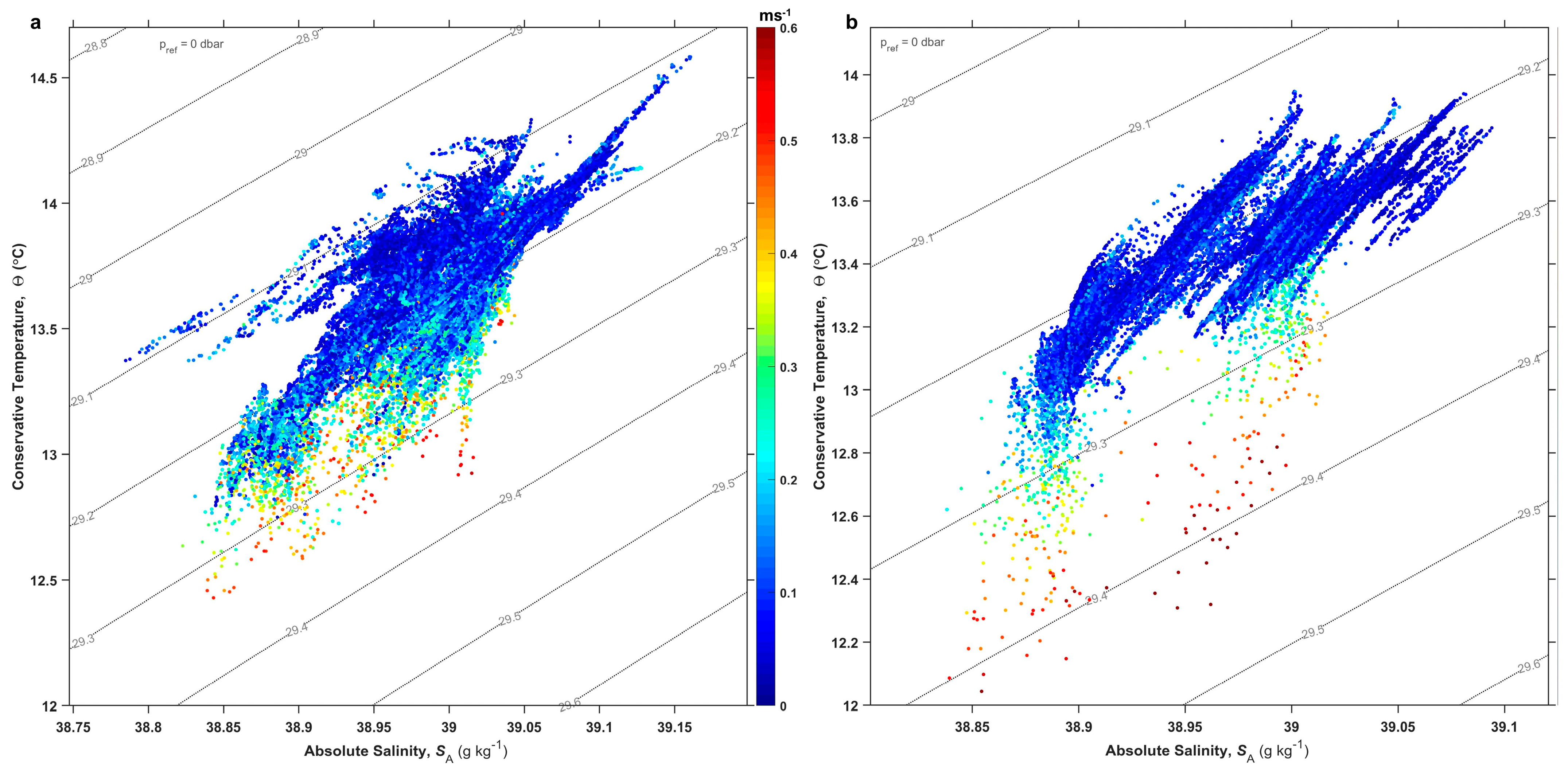
3.1. Thermohaline Records

The thermohaline properties of seawater were measured at the two mounting depths of the CTD and ADCP probes (10 and 100 m above the seafloor—mab). The time series of BB and FF used for Figure 2 and Figure 3 both start in March 2012 during the cascade event [37], triggered by the extreme cold event in the northern Adriatic Sea, which is well known in the literature.
The records at the two sites show variations in thermohaline parameters at monthly and annual scales. Along the time series, pronounced fluctuations consistently occur during the winter–spring period (February–April) (Figure 2) and vary in intensity from year to year (Figure 3). The most pronounced events (besides 2012) occurred in 2013, 2017, and 2018. While the fluctuations in the average trend are small, the fluctuations in the standard deviation and the minimum and maximum values are clearly visible (Figure 2 and Figure 3).
Temperature and salinity drop during the winter–spring months are more pronounced near the bottom, especially at FF, while vertical differences are less pronounced at BB. The overall trend of temperature and salinity is positive during the period of record. The increasing trend of the annual mean can be seen in Figure 3, as well as in the entire time series of Paladini de Mendoza et al. [53], and this hypothesis will be discussed and tested in more detail later in this section. This trend is particularly evident in the salinity records, where the average increase in salinity between 2012 and 2020 is more than 0.1.
Because the concurrent ADCP and CTD records begin in 2012, the year in which an intense cascading event occurred, this observed positive trend could be influenced by the presence of this event early in the time series. Therefore, to better assess the presence or absence of an actual trend, the extended CTD time series from 2010 to 2020 was used (Figure 4).
The nonparametric Mann–Kendall test [55,56] is used to evaluate the significance of the monotonic trend in annual mean temperature and salinity at BB. The test is applied considering a significance level of 0.05 (p-val), and the obtained results are 0.0195 for temperature and 9.9219 × 10⁻⁵ for salinity, indicating the presence of a positive trend with statistical significance.

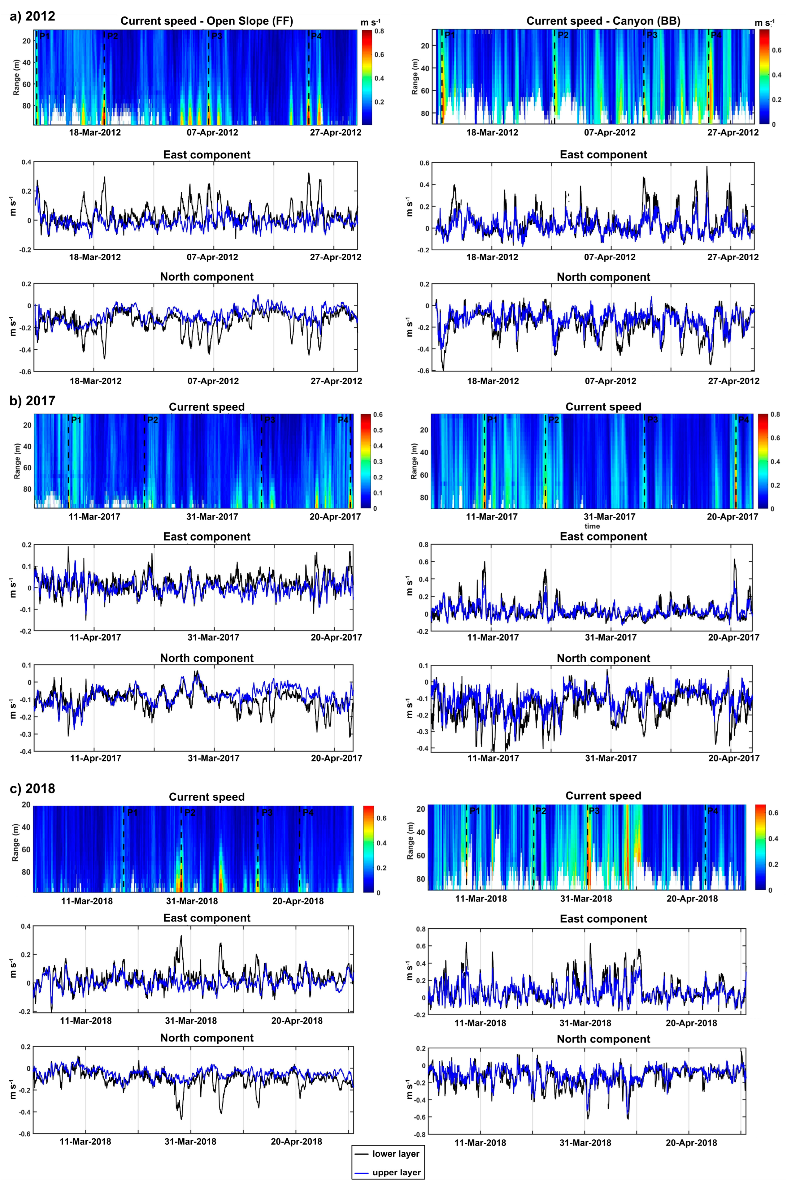
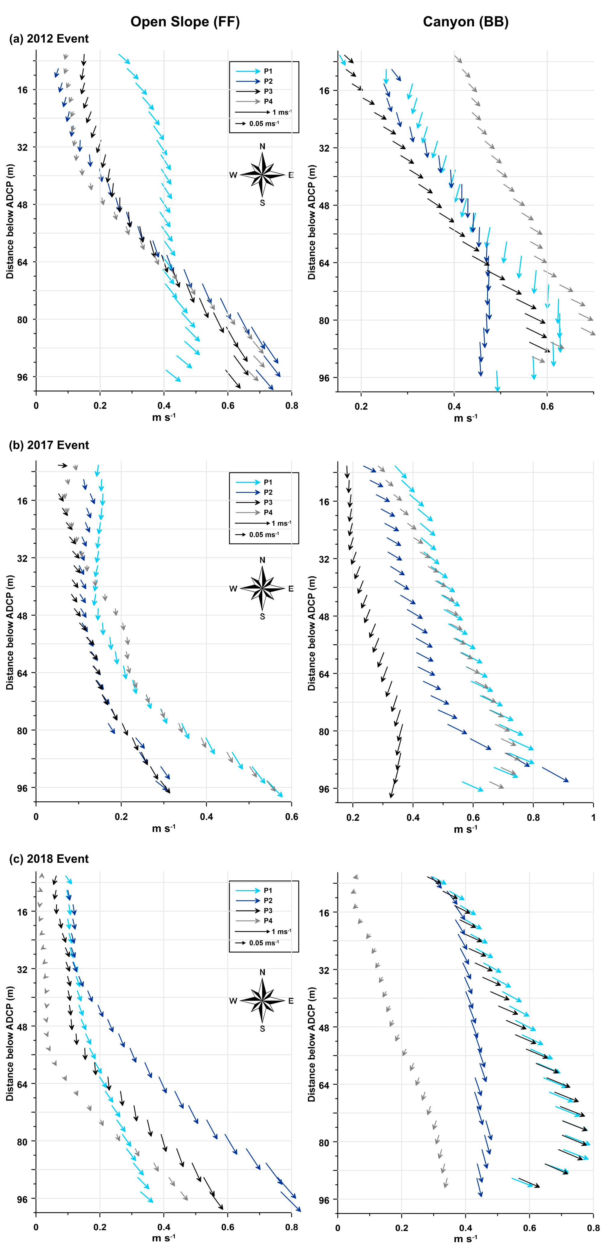
3.2. Hydrodynamic Records
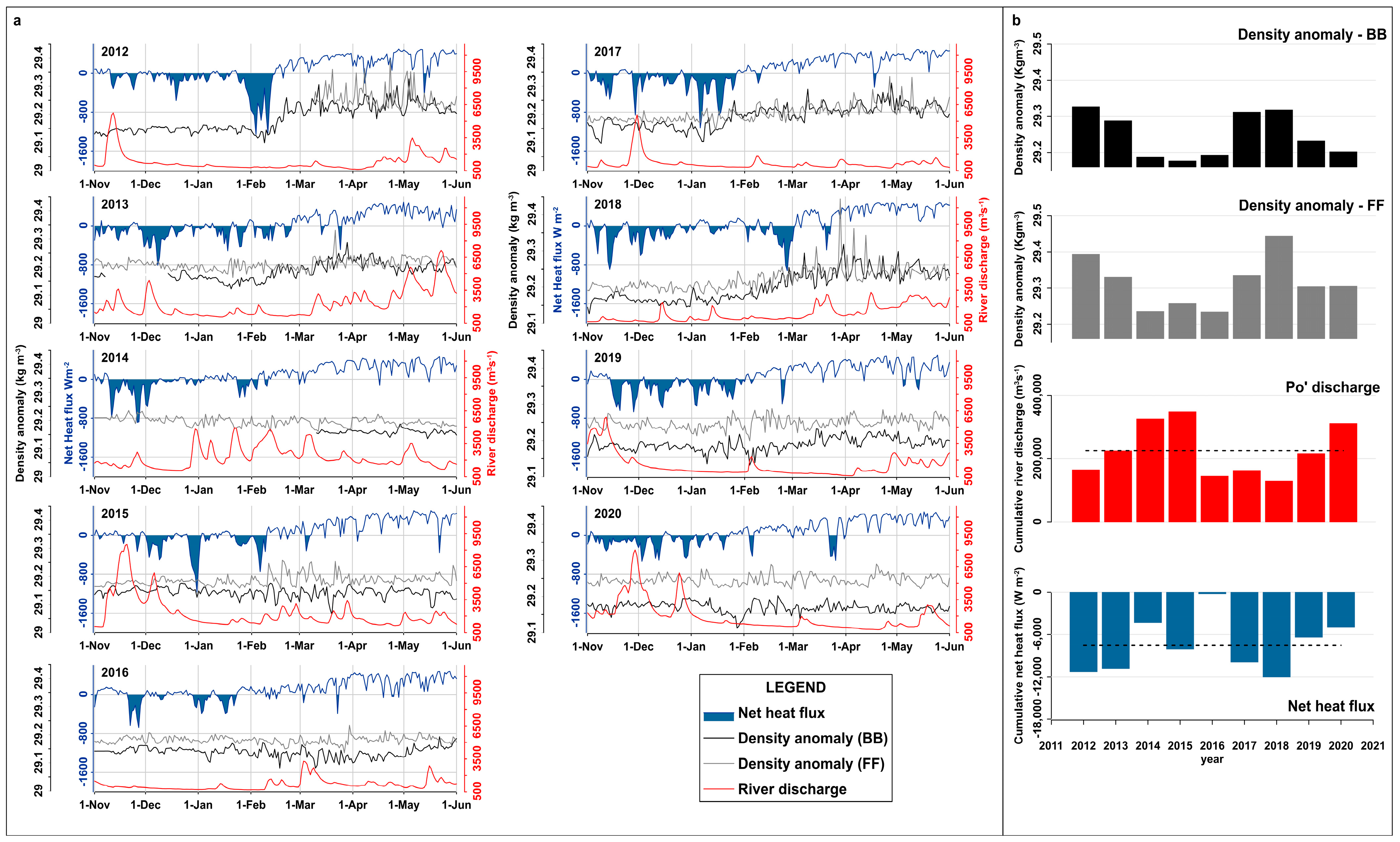
At the mooring sites, the extended hydrodynamic records from 2012 to 2020 show a generally weak velocity field (less than 0.1 m s−1) with episodic flow pulsations that may exceed 0.5 m s−1. Figure 5a and Figure 6a show calculations of the monthly and annual mean and standard deviations of the current velocity for each cell depth. Between July and January, the flow velocity field is weak, while between February and June there is an increase in velocities (Figure 5) and the flow velocity increases between 428 and 1085% of the mean velocity during pulsations. The higher standard deviation values in the lower layers testify to greater variability in the velocity field near the bottom.
At the BB site, the flow pulses near the bottom have a maximum velocity of 0.76 m s−1 and are directed to the southeast (Figure 5a,c). At the FF site, the flow moves down the slope toward the southeast and can reach velocities of up to 0.79 m s−1 (Figure 5b,d). During these pulses, the change in flow velocity ranges from 600 to 1560% of the average velocity. At the BB site (Figure 5a), the high standard deviation values are found in a thick layer of the observed water column (50–60 m), while at the FF site they are limited to a thin layer near the bottom (about 10–20 m).
The bottom layer observations plotted in the polar scatter plot in terms of direction and speed (Figure 5c,d) show that the pulsations at the FF site are characterized by southeast-oriented currents, while the BB site is characterized by bimodality of the flow direction during the months of current velocity intensification.
In the different years of observation, average annual flow velocity varies without a clear temporal trend, ranging from 0.02 to 0.15 m s−1 (Figure 6). In Figure 6a,b, we see years with higher flow velocities (2012, 2013, 2017, 2018) and years with a weaker velocity field (2014, 2015, 2016, 2019, 2020). As on the monthly scale at the BB site (Figure 6a), the currents exhibit velocity variations that include a thicker layer, and the standard deviation indicates high variability with comparable flow velocity between the two sites (Figure 6a,b).
When events are grouped into “strong” and “weak” years (Figure 6c,d), the differences between the two hydrodynamic regimes become clear. Flows with velocities greater than 0.3 m s−1 in the direction of the canyon axis in BB and those with velocities greater than 0.2 m s−1 in the southeast direction in FF are completely absent in “weak” years.
The climate of the currents during the two conditions of higher and lower velocity fields at the measurement sites is represented by the probability of the occurrence of events in the polar histogram created by grouping the events according to specific velocity and direction intervals (see legend in Figure 7). At the BB site (Figure 7, top), south-oriented flows dominate, while southeast-oriented flows are the fastest. The latter are energetic but have low abundance in all years except 2018, when they reach a maximum. In the weak years shown at the top of Figure 7a, velocities are low and characterized by opposing flows along the NW and SE axes. At the FF site (Figure 7, bottom), the velocity field is generally dominated by weak southerly currents, which are joined by the strong pulses of southeast-oriented currents in the most energetic years (strong years in Figure 7a, bottom).
The intra-annual climatology of the two different periods (January–June and July–December) can also be seen in detail in Figure 7b.
At the BB site (Figure 7b top), the high variability in dynamics during the year is immediately noticeable. From February to April, the currents exhibit a strong southeasterly component (>0.4 m s−1), which decreases during the rest of the year. Strong southward currents (>0.4 m s−1) occur from February to July, but this flow remains fairly constant in each month, reaching an intermediate level of intensity (0.2–0.4 m s−1). The least energetic months are November and December, when the flow has two main directions: northwest and southeast. This weak northwesterly component (<0.2 m s−1) is always present but is dominant only in calm months.
At the FF site (Figure 7b, bottom), southward flow is dominant throughout the year, with velocities generally below 0.2 m s−1. The directional spread of currents is mainly confined in the second and third quadrants and becomes narrower between March and May, when the dominant currents (velocity > 0.4 m s−1) are concentrated to the southeast. In November and December, the velocity field is weakest with a broader directional extent, still directed southward.

4. Discussion

4.1. Characteristics of DW Cascading Events

The characteristics of the water masses cascading down the slope (FF site) and down the canyon (BB site) are clearly highlighted by linking the flow velocity data to the thermohaline properties measured at the ADCP and CTD mooring depths, respectively. A clear overview of the dynamic processes is provided by in the polar diagrams in Figure 8, which show flow direction and velocity associated with the corresponding temperature (Figure 8a) and salinity (Figure 8b) data.
The plots show that the flow pulsations are characterized by low temperature and salinity values. In particular, at the BB site, the coldest and less saline currents rapidly cascade down the canyon, just as at the FF site where the flow cascading down the slope toward the southeast is the coldest and less saline. These fluctuations are evident at 10 m from the bottom, while they are almost absent at 100 m from the bottom at site FF and less pronounced at site BB. The T-S diagram in Figure 9 characterizes the water mass in relation to the flow velocity for each record and clearly shows the higher density of water during the flow pulses.
A velocity threshold of 0.2 m s−1 was used to select DW cascade events based on the differences observed in the polar scatter plots in Figure 6d between high-energy months (January–June) and low-energy months (July–December) at the FF site. The same velocity threshold was chosen to compare the two sites and the number of events was counted for each year, with the count at FF referring only to the second quadrant, while at BB two directional sectors with southerly and southeasterly flow are distinguished. The results presented in Table 1 show considerable annual variation and differences among sites. Threshold exceedances occur on average for 19.7 (BB) and 3.2 (FF) days per year at the sites, with a higher frequency of exceedances (6%) at BB than at FF, where exceedances average 1% of total records. At BB, the only events from the southeast associated with cascading [41] account for 0.9%, while flow from the south is more frequent (5.1%). Annual variability shows events ranging from 0 to 16% in frequency at BB, while the frequency at FF is much lower (0–5%). In 2012, both sites were affected by the longest period of DW current passage (41.2 days at BB and 14.9 days at FF).
This difference in frequency can be explained by the depth of the monitoring site. The mooring of BB is located at a depth of 600 m and is more likely to be affected by less dense currents than those that can reach the greater depth of FF. However, the water masses that can move rapidly down the canyon axis are those that are in buoyancy disequilibrium and are therefore much colder and denser than the others, thus reaching the greatest depths and therefore occurring with comparable frequency at the two monitoring sites.
The conditions shown in Figure 10a–c illustrate the hydrodynamics during the cascading events. At both sites, the hydrodynamics are characterized by intermittent pulses that propagate along the water column in different ways. As observed during the 2012 short-term observations [41], the pulses occur more frequently at the FF site and are confined to a narrow layer near the bottom. In contrast, at the BB site, they have a longer period and cover a greater thickness of the water column. The northern and eastern components of the flow at BB have negative and positive values, respectively, during acceleration and differ little between the upper and lower layers. In contrast, the values of the components in FF are very weak in the upper layer, while sharp peaks occur in the lower layer, indicating the clear southeasterly motion of the flow.
The pulses during cascading events (Figure 10) at BB last for several days (3 days) and include a water column thickness of up to 80 m above the bottom. At the FF site, pulses are more concentrated near the bottom (30–50 m) and last for a shorter period of time (1–2 days). The timing of these dense flow pulses has been defined previously [41] and is also found in the other cascading events recorded up to 2020. At the FF site, the multiple short-lived pulses are associated with trains of Continental Shelf Waves, which behave differently between sites due to the geometric constraints of the bottom topography [57].
The DW production area is the northern part of the Adriatic Sea, where several factors can come together in winter [18,58,59]. Unlike other DW production areas (e.g., the Gulf of Lion) where the production area and the shelf edge are very close to each other, DW in the Adriatic Sea is observed along the southern margin with a significant delay due to the distance from the DW production area. In 2012, for example, the first DW pulses were observed as early as three weeks after their onset in February [21], and in the other years when cascading events occurred, they were also observed mainly between February and March after the negative changes in heat flux during the winter period in the northern Adriatic. In a previous study [41], a high lag correlation between sites was observed, showing that the dense flow on the shelf primarily reaches the FF site and then the BB site after a lag of 72 h.
This result relates to analysis of the 2012 event, and when we repeated this cross-correlation analysis for the eastern component of the lower layer (black line) for the 2017 and 2018 events (the extension of the analyzed time series is shown in Figure 10), we found the same behavior with a significant correlation of 0.81 and 0.76 between BB and FF, respectively, and a time lag between the sites of between 42.5 and 64 h. During cascading, the downward dense vein mixes with ambient water, leading to progressive thickening of the downward flow and dilution of the original thermohaline properties due to entrainment of ambient water [10,41]. The vertical profiles extracted in agreement with the flow peaks provide a detailed insight into the vertical dynamics of the flow at the two mooring sites and highlight some characteristic features of the sites (Figure 11). At BB, the flow along the water column generally increases toward the seafloor and maintains a constant direction without rotation. In contrast, at the FF site, flow rotates along the water column and velocity increases steeply near the seafloor in a layer with a variable width of between 20 and 55 m. In the upper layer of FF, the velocity rarely exceeds 0.2 m s−1, while at the BB site the flow pulses extend over a thicker layer of the water column (10–90 m), with the maximum velocity sometimes concentrated a few meters above the seafloor (between 12 and 16 m).

4.2. Linkage between Cascading Events and Preconditioning Factors

The interannual variability in the cascading process is related to the formation of DW, which is seasonal, episodic, and forced by weather conditions, combined with preconditions such as low river discharge [42], which causes increased salinity at all sites of DW formation. The intrusion of cold atmospheric air is associated with Bora events, i.e., northerly winds that, when sustained for more than ten consecutive days, promote DW formation.
The potential density anomaly recorded at the two moorings (Figure 1b) during the fall–winter period was observed simultaneously with the Po’ river discharge and the net surface heat flux of the northern Adriatic Sea (DW formation area, Figure 1a). The Po’ river discharge data were obtained from the Pontelagoscuro hydrological monitoring station of ARPA Emilia-Romagna (Figure 12a), while the daily surface heat flux data were extracted from Copernicus Climate ERA-5 at the individual level (Copernicus climate data store, DOI: 10.24381/cds.adbb2d47). The daily time series of potential density anomalies, river discharge, and net heat flux between November and June of each year are shown in Figure 12. The time series of potential density anomalies begin in March 2012 for the FF site and in 2011 for the BB site. Figure 12 shows that the net heat flux is generally negative during the months of November through March, with considerable variation between years. Net heat flux is an indicator of fall–winter conditions and is particularly related to the frequency and intensity of northern storms, which bring in cold and dry air that strongly influences heat loss by causing negative spikes in the time series. The graphs show that 2016 was a particularly mild year, while there were particularly intense events in 2012, 2015, 2017, and 2018 that caused a net negative heat flux of less than 800 Wm−2. The discharge of the Po’ River also exhibits pronounced interannual variability. In particular, in 2012, 2016, 2017, and 2018, discharge remained consistently low throughout the fall–winter period, while it was higher in 2014, 2015, and 2020. Potential density anomalies recorded near the seafloor indicate that density increases, if present, are generally triggered beginning in February after the negative phase of heat flow. Figure 12b summarizes what was observed in panel a of the same figure about the variability in the parameters observed in the different years. The Po’ discharge and heat fluxes were accumulated between November and March, while the density data describe the maximum value reached near the bottom at the locations of the two moorings. The resulting trends help explain the interannual variability observed in the cascading events.
From the graphs in Figure 12b, it is clear that 2012 was a year of high heat loss combined with below-average river discharge. Similarly, in 2017 and 2018, both heat loss and lower river discharge were more pronounced; in particular, in 2018, the maximum density values at the FF station reached the highest values, while the values at the BB station were comparable to those of 2012. In 2013, heat loss was higher than average, but this condition was accompanied by river discharge close to average values. A hydrologic deficit can also be seen in 2016 and 2019, but net heat fluxes were very different in those years. In 2016, net heat flux loss was near zero, while net heat flux loss in 2019 was higher but lower than average. In 2014, 2015, and 2020, the density anomaly did not change significantly, and these years were characterized by high river run-off and below-average or near-average heat loss.
In summary, the combination of heat losses in the NAdDW production area in the northern Adriatic caused by northern winds and the hydrological conditions of the Po’ River play a key role. Under similar heat loss conditions, the occurrence of dense flows is observed in years with below-average discharge, clearly confirming what has been shown in previous studies [18,42].

5. Conclusions

Observations in the last 100 m of the water column made with the two moorings on the western edge of the southern Adriatic shelf have produced one of the most comprehensive time series on the dynamics of the deep sea in the Mediterranean. The two moorings, located at 600 and 700 m depth, respectively, on the main branch of the BCS and in an open slope area, are located in a hotspot for the passage of dense currents cascading down the continental slope. The long-term observations presented here have defined dynamics in terms of the inter- and intra-annual characteristics of dense currents and present differences in dynamics behavior between the observation sites. The deep-water dynamics are characterized by a predominant velocity field of weak intensity (<0.1 m s−1), which is interrupted almost annually by increasing velocities due to episodic flow pulsations that can reach velocities of more than 0.5 m s−1. The water masses that form these currents are colder, less salty, and denser than during other months of the year. These currents flow downslope in specific directions during a window of about 6 months, peaking between February and May, and may extend into June, gradually weakening. DW cascading events have only occurred in a few years (2012, 2013, 2017, 2018), and no specific temporal trend has been identified to date. In contrast to hydrodynamic conditions, which show no temporal trends, thermohaline conditions recorded from 2010 to 2020 show positive trends in temperature and salinity. There is increasing evidence that water masses in the Mediterranean Sea are becoming warmer and saltier [59]. In particular, the deep southern Adriatic Sea shows centennial warming (1911–2009, [60]), and periods of exceptionally high salinity have recently been observed in the Adriatic basin [51]. The importance of this aspect requires future dedicated studies.
The DW passage represents a very limited portion of the dataset. A quantitative estimate of events with velocities greater than 0.2 m s−1 yielded an average of 3.2 and 19.7 days per year for the FF and BB sites, respectively. These averages varied considerably from year to year, ranging from a maximum of 40 (BB) and 15 days (FF) depending on the duration of the cascading event. In addition to these general characteristics, the two sites also exhibit site-specific dynamic characteristics that have never been defined before. The current climate at BB exhibits a trimodality of flow directions that is dominant toward the south, has greater velocity toward 110° N along the canyon axis, and has a third, smaller component toward the northeast. The southerly flow is absent during calmer years and months (November and December), and during this time the third northwesterly flow along with the southeasterly flow dominates the hydrodynamic conditions, with very weak currents moving along the canyon axis.
At the FF site, the current climate is dominated by constant southerly currents propagating in a wide range of directions during periods characterized by a weak velocity field, while during DW passage strong currents pulse in a narrow directional sector dominated by southeasterly flow (140–150° N).
The BB site is generally characterized by a stronger velocity field than the FF site, not in terms of the maximum velocity of currents, but in terms of the number of events. However, analysis of cascading events at the BB site has shown that the frequency of flows along the canyon directly related to the cascading process is the same (about 1%) as at the FF site.
The variability in preconditioning factors observed in the fall and winter of each year showed a clear relationship with the formation of DW in the northern Adriatic basin and the subsequent cascading along the continental margin. The years when the cascading process was clearly observed correspond to the years when the largest heat losses occurred in the northern sector in combination with lower river inputs, showing that the combined effect of preconditioning factors, together with their variability, is crucial for the dynamics of the cascading process. DW plays a key role in water renewal in the northern Adriatic and oceans in general, and deep-water dynamics and its link to atmospheric events and hydrology, which are sensitive factors for extreme events, are sensitive issues in a global change scenario. Future work can further investigate the dynamics of DW along the Adriatic basin as a function of the combination of preconditioning factors using the time series generated by observational activities between the northern and southern basins of the Adriatic Sea through multidisciplinary work that brings together the activity of different research groups. Continuous observational activities over time are essential for observing and analysing the climatological evolution of the phenomenon, which is difficult to capture with only sporadic oceanographic surveys due to its elusive nature and impact on the dynamics and equilibrium of marine ecosystems.

Author Contributions

Conceptualization, F.P.d.M., K.S., L.L. and S.M.; methodology, F.P.d.M., L.L., K.S., P.G., S.M. and J.C.; investigation, S.M., L.L., M.B. and P.G.; data curation, F.P.d.M., J.C. and K.S.; writing—original draft preparation, F.P.d.M., K.S., L.L., S.M. and P.G.; writing—review and editing, all authors; supervision, K.S., L.L., P.G. and J.C.; project administration, K.S., L.L., S.M. and P.G.; funding acquisition, K.S., L.L., S.M. and P.G. All authors have read and agreed to the published version of the manuscript.

Funding

This research was funded by the PRIN-PASS project (PRIN: Progetti di Ricerca di Rilevante Interesse Nazionale—Bando 2017—Prot.n. 2017ASZAKJ). The maintenance of the BB and FF fixed moorings over time was only possible due to the support of the following projects: the European Community’s Seventh Framework Programme projects “Hotspot Ecosystem Research and Man’s Impact on European seas” (HERMIONE; grant agreement no. 226354) and “Towards Coast to COast NETworks of marine protected areas (from the shore to the high and deep sea), coupled with sea-based wind energy potential” (COCONET; grant agreement no. 287844), as well as the RITMARE (Italian Research for the Sea; grant no. SP5_WP3_AZ1) flagship project. This work was also supported by a grant from Istituto Nazionale di Geofisica e Vulcanologia within the framework of the Joint Research EMSO Italia through funds devoted by the Italian Ministry of University and Research to international dimension activities linked to the European Research Infrastructure EMSO and by a grant from the Ufficio Programmazione e Grant Office of CNR-Italy (CNR-UPGO).

Institutional Review Board Statement

Not applicable.

Informed Consent Statement

Not applicable.

Data Availability Statement

All data are made publicly available through the Zenodo repository. The registered database DOI is https://doi.org/10.5281/zenodo.6770201 (Paladini Mendoza et al., 2022).

Acknowledgments

The authors thank the reviewers for helpful comments that substantially improved the final version of the paper. We are also grateful to the cruise participants who helped us with the mooring servicing, in particular the captain and the crew members of the R/V Urania, R/V Minerva Uno, R/V G. Dallaporta, R/V Laura Bassi, and R/V OGS Explora, as well as the fishing boats Pasquale & Cristina and Attila.

Conflicts of Interest

The authors declare no conflict of interest.

References

  1. Bertotti, G.; Casolari, E.; Picotti, V. The Gargano Promontory: A Neogene contractional belt within the Adriatic plate. Terra Nova 1999, 11, 168–173. [Google Scholar] [CrossRef]
  2. Ridente, D.; Trincardi, F. Eustatic and tectonic control on deposition and lateral variability of Quaternary regressive sequences in the Adriatic basin (Italy). Mar. Geol. 2002, 184, 273–293. [Google Scholar] [CrossRef]
  3. Bonaldo, D.; Benetazzo, A.; Bergamasco, A.; Campiani, E.; Foglini, F.; Sclavo, M.; Trincardi, F.; Carniel, S. Interactions among Adriatic continental margin morphology, deep circulation and bedform patterns. Mar. Geol. 2016, 375, 82–98. [Google Scholar] [CrossRef]
  4. Minisini, D.; Trincardi, F.; Asioli, A. Evidence of slope instability in the Southwestern Adriatic Margin. Nat. Hazards Earth Syst. Sci. 2006, 6, 1–20. [Google Scholar] [CrossRef]
  5. Martorelli, E.; Falcini, F.; Salusti, E.; Chiocci, F. Analysis and modeling of contourite drifts and contour currents off promontories in the Italian Seas (Mediterranean Sea). Mar. Geol. 2010, 278, 19–30. [Google Scholar] [CrossRef]
  6. Verdicchio, G.; Trincardi, F. Short-distance variability in slope bed-forms along the Southwestern Adriatic Margin (Central Mediterranean). Mar. Geol. 2006, 234, 271–292. [Google Scholar] [CrossRef]
  7. Trincardi, F.; Verdicchio, G.; Miserocchi, S. Seafloor evidence for the interaction between cascading and along-slope bottom water masses. J. Geophys. Res. 2007, 112, F03011. [Google Scholar] [CrossRef] [Green Version]
  8. Verdicchio, G.; Trincardi, F.; Asioli, A. Mediterranean bottom-current deposits: An example from the Southwestern Adriatic Margin. Geol. Soc. Lond. Spec. Publ. 2007, 276, 199–224. [Google Scholar] [CrossRef]
  9. Turchetto, M.; Boldrin, A.; Langone, L.; Miserocchi, S.; Tesi, T.; Foglini, F. Particle transport in the Bari Canyon (southern Adriatic Sea). Mar. Geol. 2007, 246, 231–247. [Google Scholar] [CrossRef]
  10. Rubino, A.; Romanenkov, D.; Zanchettin, D.; Cardin, V.; Hainbucher, D.; Bensi, M.; Boldrin, A.; Langone, L.; Miserocchi, S.; Turchetto, M. On the descent of dense water on a complex canyon system in the southern Adriatic basin. Cont. Shelf Res. 2012, 44, 20–29. [Google Scholar] [CrossRef]
  11. Pinardi, N.; Estournel, C.; Cessi, P.; Escudier, R.; Lyubartsev, V. Dense and deep water formation processes and Mediterranean overturning circulation. In Oceanography of the Mediterranean Sea, An Introductory Guide; Schroeder, K., Chiggiato, J., Eds.; Elsevier Inc.: Amsterdam, The Netherlands, 2022; pp. 209–252. ISBN 978-0-12-823692-5. [Google Scholar]
  12. Ivanov, V.V.; Shapiro, G.I.; Huthnance, J.M.; Aleynik, D.L.; Golovin, P.N. Cascades of dense water around the world ocean. Prog. Oceanogr. 2004, 60, 47–98. [Google Scholar] [CrossRef]
  13. Hendershott, M.C.; Rizzoli, P. The winter circulation of the Adriatic Sea. Deep-Sea Res. 1976, 23, 353–370. [Google Scholar] [CrossRef]
  14. Franco, P.; Jeftic, L.; Rizzoli, P.M.; Miehelato, A.; Orlic, M. Descriptive model of the Northern Adriatie. Oceanol. Acta 1982, 5, 379–389. [Google Scholar]
  15. Foglini, F.; Campiani, E.; Trincardi, F. The reshaping of the South West Adriatic margin by cascading of dense shelf waters. Mar. Geol. 2016, 375, 64–81. [Google Scholar] [CrossRef]
  16. Tesi, T.; Langone, L.; Goñi, M.A.; Turchetto, M.; Miserocchi, S.; Boldrin, A. Source and composition of organic matter in the Bari canyon (Italy): Dense water cascading vs particulate export from the upper ocean. Deep-Sea Res. I Oceanogr. Res. Pap. 2008, 155, 813–831. [Google Scholar] [CrossRef]
  17. Langone, L.; Conese, I.; Miserocchi, S.; Boldrin, A.; Bonaldo, D.; Carniel, S.; Chiggiato, J.; Turchetto, M.; Borghini, M.; Tesi, T. Dynamics of particles along the western margin of the Southern Adriatic: Processes involved in transferring particulate matter to the deep basin. Mar. Geol. 2016, 375, 28–43. [Google Scholar] [CrossRef]
  18. Vilibic, I. An analysis of dense water production on the North Adriatic shelf, Estuar. Coast. Shelf Sci. 2003, 56, 697–707. [Google Scholar] [CrossRef]
  19. Vilibic, I.; Grbec, B.; Supic, N. Dense water generation in the north Adriatic in 1999 and its recirculation along the Jabuka Pit. Deep. Sea Res. Part I 2004, 51, 1457–1474. [Google Scholar] [CrossRef]
  20. Bignami, F.; Salusti, E.; Schiarini, S. Observations on a bottom vein of dense water in the Southern Adriatic and Ionian Seas. J. Geophys. Res. 1990, 95, 7249–7259. [Google Scholar] [CrossRef]
  21. Benetazzo, A.; Bergamasco, A.; Bonaldo, D.; Falcieri, F.M.; Sclavo, M.; Langone, L.; Carniel, S. Response of the Adriatic Sea to an intense cold air outbreak: Dense water dynamics and wave-induced transport. Prog. Oceanogr. 2014, 128, 115–138. [Google Scholar] [CrossRef]
  22. Zore-Armanda, M. Les masses d’eau de la mer Adriatique. Acta Adriat. 1963, 10, 5–88. [Google Scholar]
  23. Artegiani, A.; Bregant, D.; Paschini, E.; Pinardi, N.; Raicich, F.; Russo, A. The Adriatic Sea General Circulation. Part I: Air-sea interactions and water mass structure. J. Phys. Oceanogr. 1997, 27, 1492–1514. [Google Scholar] [CrossRef]
  24. Orlic, M.; Gacic, M.; La Violette, P.E. The currents and circulation of the Adriatic Sea. Oceanol. Acta 1992, 15, 109–124. [Google Scholar]
  25. Vilibić, I.; Pranić, P. Denamiel, North Adriatic Dense Water: Lessons learned since thepioneering work of Mira Zore-Armanda 60 years ago. Acta Adriat. 2023, 64, 53–78. [Google Scholar] [CrossRef]
  26. Manca, B.B.; Ibello, V.; Pacciaroni, M.; Scarazzato, P.; Giorgetti, A. Ventilation of deep waters in the Adriatic and Ionian Seas following changes in thermohaline circulation of the Eastern Mediterranean. Clim. Res. 2006, 31, 239–256. [Google Scholar] [CrossRef]
  27. Rovere, M.; Pellegrini, C.; Chiggiato, J.; Campiani, E.; Trincardi, F. Impact of dense bottom water on a continental shelf: An example from the SW Adriatic margin. Mar. Geol. 2019, 408, 123–143. [Google Scholar] [CrossRef]
  28. Pirro, A.; Mauri, E.; Gerin, R.; Martellucci, R.; Zuppelli, P.; Poulain, P.M. New Insights on the Formation and Breaking Mechanism of Convective Cyclonic Cones in the South Adriatic Pit during Winter 2018. In Proceedings of the EGU General Assembly 2023, Vienna, Austria, 24–28 April 2023. [Google Scholar] [CrossRef]
  29. Cardin, V.; Wirth, A.; Khosravi, M.; Gacic, M. South Adriatic Recipes: Estimating the Vertical Mixing in the Deep Pit. Front. Mar. Sci. 2020, 7, 565982. [Google Scholar] [CrossRef]
  30. Bensi, M. Thermohaline Variability and Mesoscale Dynamics Observed at the E2M3A Deep-Site in the South Adriatic Sea. Ph.D. Thesis, Università Degli Studi di Trieste, Trieste, Italy, 2012. Available online: https://www.openstarts.units.it/handle/10077/7387 (accessed on 29 June 2023).
  31. Bensi, M.; Cardin, V.; Rubino, A. Thermohaline Variability and Mesoscale Dynamics Observed at the Deep-Ocean Observatory E2M3A in the Southern Adriatic Sea, in the Mediterranean Sea: Temporal Variability and Spatial Patterns, Geophysical Monograph Series; Borzelli, G.L.E., Gačić, M., Lionello, P., Malanotte-Rizzoli, P., Eds.; John Wiley & Sons, Inc.: Oxford, UK, 2014; pp. 139–155. [Google Scholar]
  32. Cardin, V.; Bensi, M. E2m3a-2006-2010-Time-Series-Southadriatic; OGS (Istituto Nazionale di Oceanografia e di Geofisica Sperimentale), Division of Oceanography: Trieste, Italy, 2014. [Google Scholar] [CrossRef]
  33. Cardin, V.; Bensi, M.; Siena, G.; Ursella, L. E2m3a2011-2013-Timeseries-Southadriatic; OGS (Istituto Nazionale di Oceanografia e di Geofisica Sperimentale), Division of Oceanography: Trieste, Italy, 2014. [Google Scholar] [CrossRef]
  34. Cardin, V.; Bensi, M.; Ursella, L.; Siena, G. E2m3a2013-2015-Time-Series Southadriatic; OGS (Istituto Nazionale di Oceanografia e di Geofisica Sperimentale), Division of Oceanography: Trieste, Italy, 2015. [Google Scholar] [CrossRef]
  35. Cardin, V.; Bensi, M.; Brunetti, F.; Conese, I.; Giani, M.; Langone, L. A Multidisciplinary Observing System to Understand Oceanographic Processes in the Open Adriatic Sea. Rapp. Comm. Int. Mer Médit. 2016, 41, 115. [Google Scholar]
  36. Cardin, V.; Bensi, M.; Ursella, L.; Siena, G. E2m3a2015-2017-Timeseries-Southadriatic; OGS (Istituto Nazionale di Oceanografia e di Geofisica Sperimentale), Division of Oceanography: Trieste, Italy, 2018. [Google Scholar] [CrossRef]
  37. Chiggiato, J.; Schroeder, K.; Trincardi, F. Cascading dense shelf-water during the extremely cold winter of 2012 in the Adriatic, Mediterranean Sea: Formation, flow, and seafloor impact—Preface. Mar. Geol. 2016, 375, 1–4. [Google Scholar] [CrossRef]
  38. De Santis, A.; Chiappini, M.; Marinaro, G.; Guardato, S.; Conversano, F.; D’Anna, G.; Di Mauro, D.; Cardin, V.; Carluccio, R.; Rende, S.F.; et al. InSEA Project: Initiatives in Supporting the Consolidation and Enhancement of the EMSO Infrastructure and Related Activities. Front. Mar. Sci. 2022, 9, 846701. [Google Scholar] [CrossRef]
  39. Ravaioli, M.; Bergami, C.; Riminucci, F.; Langone, L.; Cardin, V.; Di Sarra, A.; Aracri, S.; Bastianini, M.; Bensi, M.; Bergamasco, A.; et al. The RITMARE Italian Fixed Point Observatory Network (IFON) for marine environmental monitoring: A case study. J. Oper. Oceanogr. 2016, 9, s202–s214. [Google Scholar] [CrossRef] [Green Version]
  40. Paladini de Mendoza, F.; Schroeder, K.; Langone, L.; Chiggiato, J.; Borghini, M.; Giordano, P.; Verazzo, G.; Miserocchi, S. Moored current and temperature measurements in the Southern Adriatic Sea at mooring site BB and FF, March 2012–June 2020 [dataset]. Zenodo 2022. [Google Scholar] [CrossRef]
  41. Chiggiato, J.; Bergamasco, A.; Borghini, M.; Falcieri, F.M.; Falco, P.; Langone, L.; Miserocchi, S.; Russo, A.; Schroeder, K. Dense-water bottom currents in the Southern Adriatic Sea in spring 2012. Mar. Geol. 2016, 375, 134–145. [Google Scholar] [CrossRef]
  42. Mihanović, H.; Vilibić, I.; Carniel, S.; Tudor, M.; Russo, A.; Bergamasco, A.; Bubić, N.; Ljubešić, Z.; Viličić, D.; Boldrin, A.; et al. Exceptional dense water formation on the Adriatic shelf in the winter of 2012. Ocean Sci. 2013, 9, 561–572. [Google Scholar] [CrossRef] [Green Version]
  43. Marini, M.; Maselli, V.; Campanelli, A.; Foglini, F.; Grilli, F. Role of the Mid-Adriatic deep in dense water interception and modification. Mar. Geol. 2016, 375, 5–14. [Google Scholar] [CrossRef]
  44. Carniel, S.; Bonaldo, D.; Benetazzo, A.; Bergamasco, A.; Boldrin, A.; Falcieri, F.M.; Sclavo, M.; Trincardi, F.; Langone, L. Off-shelf fluxes across the southern Adriatic margin: Factors con trolling dense-water-driven transport phenomena. Mar. Geol. 2016, 375, 44–63. [Google Scholar] [CrossRef]
  45. Cantoni, C.; Luchetta, A.; Chiggiato, J.; Cozzi, S.; Schroeder, K.; Langone, L. Dense water flow and carbonate system in the southern Adriatic: A focus on the 2012 event. Mar. Geol. 2016, 375, 15–27. [Google Scholar] [CrossRef]
  46. Vilibić, I.; Zemunik, P.; Šepić, J.; Dunić, N.; Marzouk, O.; Mihanović, H.; Denamiel, C.; Precali, R.; Djakovac, T. Present climate trends and variability in thermohaline properties of the northern Adriatic shelf. Ocean Sci. 2019, 15, 1351–1362. [Google Scholar] [CrossRef] [Green Version]
  47. Buljan, M.; Zore-Armanda, M. Hydrographic data on the Adriatic Sea collected in the period from 1952 through 1964. Acta Adriat. 1966, 12, 1–438. [Google Scholar]
  48. Buljan, M.; Zore-Armanda, M. Hydrographic properties of the Adriatic Sea in the period from 1965 through 1970. Acta Adriat. 1979, 20, 1–368. [Google Scholar]
  49. Zore-Armanda, M.; Bone, M.; Dadic’, V.; Morovic’, M.; Ratkovic’, D.; Stojanoski, L.; Vukadin, I. Hydrographic properties of the Adriatic Sea in the period from 1971 through 1983. Acta Adriat. 1991, 32, 1–547. [Google Scholar]
  50. Ivankovic, D.; Dadic, V.; Srdelic, M. Marine Environmental Database of the Adriatic Sea With Application for Managing and Visualisation of Data. WIT Trans. Ecol. Environ. 2000, 41, 10. [Google Scholar] [CrossRef]
  51. Mihanović, H.; Vilibić, I.; Šepić, J.; Matić, F.; Ljubešić, Z.; Mauri, E.; Gerin, R.; Notarstefano, G.; Poulain, P.-M. Observation, Preconditioning and Recurrence of Exceptionally High Salinities in the Adriatic Sea. Front. Mar. Sci. 2021, 8, 672210. [Google Scholar] [CrossRef]
  52. Vilibić, I.; Supić, N. Dense water generation on a shelf: The case of the Adriatic Sea. Ocean. Dyn. 2005, 55, 403–415. [Google Scholar] [CrossRef]
  53. de Mendoza, F.P.; Schroeder, K.; Langone, L.; Chiggiato, J.; Borghini, M.; Giordano, P.; Verazzo, G.; Miserocchi, S. Deep-water hydrodynamic observations of two moorings sites on the continental slope of the southern Adriatic Sea (Medi-terranean Sea), Earth Syst. Sci. Data 2022, 14, 5617–5635. [Google Scholar] [CrossRef]
  54. McDougall, T.J.; Barker, P.M. Getting started with TEOS-10 and the Gibbs Seawater (GSW) Oceanographic Toolbox. Scor/Iapso WG 2011, 127, 1–28. [Google Scholar]
  55. Mann, H.B. Non-Parametric Test against Trend. Econometrica 1945, 13, 245–259. [Google Scholar] [CrossRef]
  56. Kendall, M.G. Rank Correlation Methods, 4th ed.; Charles Griffin: London, UK, 1975. [Google Scholar]
  57. Bonaldo, D.; Orlic, M.; Carniel, S. Framing Continental Shelf Waves in the southern Adriatic Sea, a further flushing factor beyond dense water cascading. Sci. Rep. 2018, 8, 660. [Google Scholar] [CrossRef] [Green Version]
  58. Vilibić, I.; Orlić, M. Adriatic water masses, their rates of formation and transport through the Otranto Strait. Deep. Sea Res. Part I 2002, 49, 1321–1340. [Google Scholar] [CrossRef]
  59. MedECC. Climate and Environmental Change in the Mediterranean Basin e Current Situation and Risks for the Future. First Mediterranean Assessment Report; Cramer, W., Guiot, J., Marini, K., Eds.; Union for the Mediterranean, Plan Bleu. UNEP/MAP: Marseille, France, 2020; p. 632. [Google Scholar] [CrossRef]
  60. Lipizer, M.; Partescano, E.; Rabitti, A.; Giorgetti, A.; Crise, A. Qualified temperature, salinity and dissolved oxygen climatologies in a changing Adriatic Sea. Ocean Sci. 2014, 10, 771–797. [Google Scholar] [CrossRef] [Green Version]
Figure 1. Study Area. (a) The Adriatic Sea and its general circulation (from Lipizer et al., 2014). The basin is divided into sub-sectors: North Adriatic (NA), Middle Adriatic (MA), and South Adriatic (SA). JP indicates the Jabuka Pit, PS the Pelagosa Sill, SAP the South Adriatic Pit, OS the Otranto Strait, and BCS the Bari Canyon System. The red box indicates the sector where moorings were deployed. The blue area indicates the NAdDW production area in the northern sector and the red diamond is the position of the hydrological station on the Po’ river, which is represented by the bolded blue line (while other main rivers on the eastern Italian coast are thin blue lines); bathymetry of panel (a) and (b) is provided by EMODNET “https://portal.emodnet-bathymetry.eu/” (accessed on 29 June 2023). (b) Details of bathymetry of the South Adriatic margin where mooring BB and FF are located in the BCS and open slope, respectively. (c) Mooring structure schemes (not in scale).
Jmse 11 01364 g001
Figure 2. Upper panel: monthly average (continuous line) and standard deviation (bar) of temperature recorded by the (a) ADCP (100 mab—blue line) and (b) CTD (10 mab—grey line) probes at the two mooring sites; dashed lines indicate minimum and maximum values. Lower panel: monthly average (continuous line) and standard deviation (bar) of salinity recorded by the CTD probe (10 mab) at the (c) BB and (d) FF sites.
Jmse 11 01364 g002
Figure 3. Upper panel: annual average (continuous line) and standard deviation (bar) of temperature recorded by the (a) ADCP (100 mab—blue line) and (b) CTD (10 mab—grey line) probes at the two mooring sites; dashed lines indicate minimum and maximum values. Lower panel: annual average (continuous line) and standard deviation (bar) of salinity recorded by the CTD probe (10 mab) at the (c) BB and (d) FF sites.
Jmse 11 01364 g003
Figure 4. Temperature (a) and salinity (b) time series recorded at site BB. The records from 2010 to 2012 are extended with a dataset from previous research [15]. Dashed lines indicate the minimum and maximum value, while continuous lines represent the mean and vertical bars indicate standard deviation.
Jmse 11 01364 g004
Figure 5. Monthly mean current speed and standard deviation of the current speed at the (a) canyon (BB) and (b) open slope site (FF). Panels (c,d) represent the polar plots of the currents in the bottom layer separated into two different month groups.
Jmse 11 01364 g005
Figure 6. Yearly mean current speed and standard deviation of the current speed (m s−1) at the (a) canyon (BB) and (b); open slope (FF) sites. Line color indicates different layers along the water column. (c,d) represent the polar plots of the currents in the bottom layer separated into two different year groups.
Jmse 11 01364 g006
Figure 7. Polar histogram plots for (a) strong and weak years and (b) the energetic period (January–July) and calm period (July–December) in the two measuring sites. The directional bins represent 5° and bar colors represent velocity in m s−1.
Jmse 11 01364 g007
Figure 8. (a) Polar scatter plot of current observations of the canyon (BB) and open slope (FF) site at two different heights along the water column and temperature. The color bar indicates the temperature measured during each observation. (b) Polar scatter plot of current observations of the BB and FF sites measured at 10 mab and salinity. The color bar indicates the salinity measured during each observation.
Jmse 11 01364 g008
Figure 9. T-S diagram calculated from conservative temperature (θ) and absolute salinity (SA) recorded by the CTD probes at the (a) canyon (BB) and (b) open slope (FF) mooring sites. The color bar indicates the intensity of currents in the layer at 10 mab during each observation.
Jmse 11 01364 g009
Figure 10. DW cascading events for 2012, 2017, and 2018 recorded at the FF (sx) and BB (dx) sites; for each event and site, the module of speed along the water column and the east and north component of the upper (blue) and lower (black) layer are represented. Dotted lines indicate the timestep where the current profiles (P1–P2–P3–P4) of Figure 11 were extracted.
Jmse 11 01364 g010
Figure 11. Profiles of current speed at the open slope (FF) (left) and canyon (BB) (right) extracted from the time series during the events in (a) 2012, (b) 2017, and (c) 2018. For each depth cell, the arrows indicate the intensity and orientation of currents. The geographical reference of vector orientation is indicated by the wind rose below the legend.
Jmse 11 01364 g011
Figure 12. (a) Daily time series of sea surface net heat flux, water density anomalies in the two mooring sites, and Po’ river discharge during the 2012–2020 recording period. The net heat flux line is filled when the value becomes negative. (b) Summary of the trends observed in the panel specified for each year. From the top, the bar plots represent the maximum density at BB and FF, the cumulative Po’ discharge, and net heat flux calculated over the autumn–winter period. Dotted lines when present indicate the average values.
Jmse 11 01364 g012
Table 1. Yearly frequency of energetic currents (current speed > 0.2 ms−1) at the two measuring sites.
YearCanyon—BBOpen Slope—FF
Southern Events (S)South-Eastern Events (SE)S + SE EventsSouth-Eastern Events
Days%Days%Days%Total RecordsDays%Total Records
201216793513.82986.22.4197741.216.212,18071314.95.113,903
201377616.24.4781.60.485417.84.917,467390.80.217,454
201460.1<0.12<0.1<0.180.2<0.117,42300017,441
2015160.30.1120.30.1280.60.217,356110.20.117,361
2016250.50.1180.40.1430.90.217,32200017,409
2017201341.911.72164.51.3222946.412.917,25333571.917,352
2018155832.59.1479102.8203742.411.917,1682465.11.417,210
2019117324.46.71473.10.8132027.57.517,491220.50.117,428
2020280.60.3000280.60.3845730.108505
Disclaimer/Publisher’s Note: The statements, opinions and data contained in all publications are solely those of the individual author(s) and contributor(s) and not of MDPI and/or the editor(s). MDPI and/or the editor(s) disclaim responsibility for any injury to people or property resulting from any ideas, methods, instructions or products referred to in the content.

