Modes of Operation and Forcing in Oil Spill Modeling: State-of-Art, Deficiencies and Challenges

Abstract

Oil spills may have devastating effects on marine ecosystems, public health, the economy, and coastal communities. As a consequence, scientific literature contains various up-to-date, advanced oil spill predictive models, capable of simulating the trajectory and evolution of an oil slick generated by the accidental release from ships, hydrocarbon production, or other activities. To predict in near real time oil spill transport and fate with increased reliability, these models are usually coupled operationally to synoptic meteorological, hydrodynamic, and wave models. The present study reviews the available different met-ocean forcings that have been used in oil-spill modeling, simulating hypothetical or real oil spill scenarios, worldwide. Seven state-of-the-art oil-spill models are critically examined in terms of the met-ocean data used as forcing inputs in the simulation of twenty-three case studies. The results illustrate that most oil spill models are coupled to different resolution, forecasting meteorological and hydrodynamic models, posing, however, limited consideration in the forecasted wave field (expressed as the significant wave height, the wave period, and the Stokes drift) that may affect oil transport, especially at the coastal areas. Moreover, the majority of oil spill models lack any linkage to the background biogeochemical conditions; hence, limited consideration is given to processes such as oil biodegradation, photo-oxidation, and sedimentation. Future advancements in oil-spill modeling should be directed towards the full operational coupling with high-resolution atmospheric, hydrodynamic, wave, and biogeochemical models, improving our understanding of the relative impact of each physical and oil weathering process.

1. Introduction

When crude oil is accidentally released in the marine environment, an oil slick is formed appearing as a thin oily layer, floating on the sea surface [1]. The slick is shaped by the slow, low-scale, and diffusive processes, responsible for changing the contaminants’ concentration, and is transported by the large-scale advective processes, advancing the center of the oil-slick mass to the direction of background currents, winds, and waves [2]. This implies that the ambient environment of the spill significantly determines its movement and fate. The amount of oil spilled in the ocean, the oil’s initial physicochemical properties, the prevailing weather and sea state conditions, and other spill-specific and environmental factors affect the timing, duration, and relative importance of each physical and biochemical oil-weathering process (known as OWP), affecting the slick [3,4,5]. Since hydrocarbons are nonconservative pollutants, OWPs cause longterm changes in their physicochemical properties, such as oil density and viscosity [6]. The most important OWPs are spreading, evaporation, dispersion/diffusion, emulsification, and dissolution. Photooxidation, biodegradation, and sedimentation act over longer time periods and determine oil’s ultimate behavior [7].

Planning for and responding to an oil spill requires rigorous comprehension of baseline environmental characteristics and processes [8]. Oil-spill models help the response agencies lessen the damaging impacts on the environment by predicting the path of at-sea oil spills. Predicting the spillage trajectory is the main outcome of oil-spill models, highlighting the potential for ecosystem harm as an incident develops, while, in parallel, assisting in the optimization of the cleanup efforts [9,10,11]. Any guidance that oil-spill modeling may offer could be extremely important for the authorities, given the tremendous effect and costs associated with oil spills. Risk evaluation, readiness planning and analysis of the environmental effects of the oil industry infrastructure, heavily rely on oil spill modeling [12]. When models are run, a wide range of input variables and actual met-ocean conditions might result in multiple alternative trajectories [13]. Following analysis, these trajectories are plotted on maps to create reaction strategies. Emergency responders must be knowledgeable about the type of oil, the location, and the marine and coastal habitats the spillage may affect. Thus, governments, oil exploration and production firms, insurance companies, and other stakeholders may evaluate whether the adequate resources, tools, and procedures are in place to respond to oil spill incidents. Simulating different scenarios may allow for assessing the potential environmental impacts and device plans on the movement of the response supplies to the necessary locations [14,15]. This procedure could lead to the assessment of the efficacy of various response strategies, as well as their benefits and drawbacks [10,12]. Additionally, it is expected to aid responders to organize and mobilize socioeconomic resources to limit environmental impacts along the oil’s potential course [8].

As explained above, met-ocean conditions, i.e., currents, wind, and waves, represent the fundamental components influencing the spreading of oil in the marine environment [7,16,17,18]. For this reason, it is crucial to be able to illustrate that oil-spill forecasts are accurate and reliable, as well as that the constraints of a model are well-understood when evaluating the model’s predicting capacity and performance [19,20]. An assessment of the ocean currents, water characteristics over the water column, and waves at a particular time and location is provided by the three-dimensional ocean-circulation models [21]. These models aid in determining how these factors will affect the transport of oil once it reaches the sea surface. Meteorological and atmospheric models provide information on air properties such as temperature, relative humidity, and barometric pressure, as well as on the surface winds that might transport and affect the evaporation rate of floating oil [22]. In parallel, wave models provide information about the significant wave height and Stokes drift fields, affecting wave turbulence, vertical mixing, and oil dispersion within the water column [23]. Furthermore, once the oil is discharged into the marine environment, the chemical and physical changes it will undergo could be predicted by the fate models [17,24].

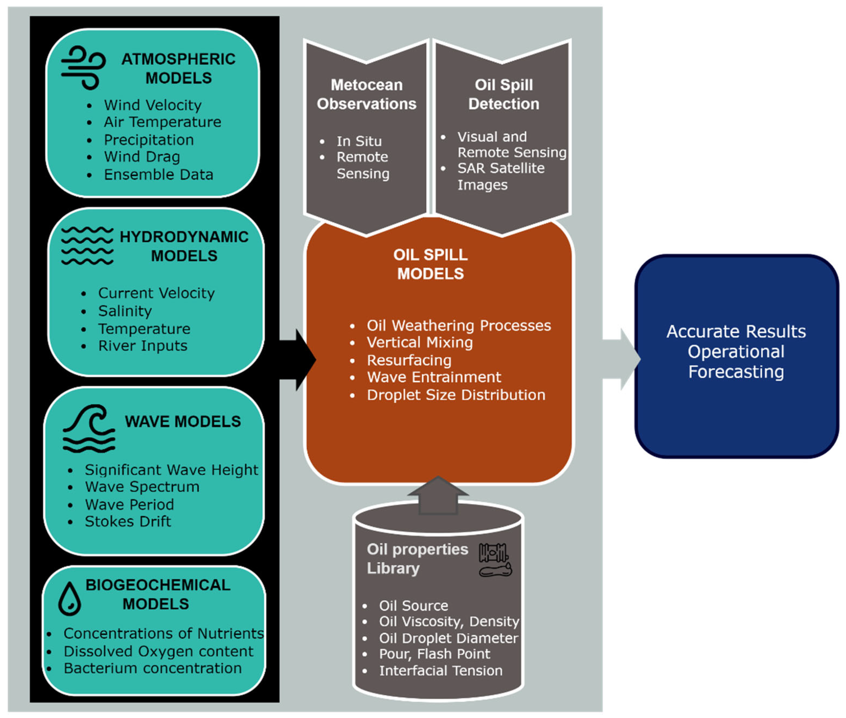
In oil-spill modeling, depending on the purpose of each simulation, the appropriate forcing data and the corresponding processes are taken into account. For example, for the transport and fate of the oil spill on the sea surface, the required forcings are the winds, sea currents, and waves and the most important processes for horizontal transport are advection, spreading, diffusion and evaporation acting in the short-term. For the vertical transport and dispersion of the oil spill, the processes that should be included are dispersion, resurfacing, vertical mixing in the short term, and biodegradation, sedimentation, and dissolution over longer time periods. Concerning deepwater oil-blowout modeling, coupled 3-D hydrodynamic models are appropriate. In addition, dissolution is a very important process in these applications, while the forcing from winds and waves seems minor. Thus, the data needs for forcing oil-spill models depend on the questions that are addressed. In general, the more complete a scenario serving different purposes with varying forcing is, the more circumstantial and comprehensive the results will be. Therefore, cutting-edge, quality-controlled, high-resolution meteorological, hydrodynamic, and wave models should be combined with oil spill models to predict accurately the fate and weathering of spilled oil at sea. Biogeochemical submodules capable of describing the fields of nutrients, carbon, and plankton are significant in determining the dominant physicochemical processes such as biodegradation, sedimentation, and photo-oxidation [7]. All of the aforementioned factors must be taken into account in operational oil-spill modeling to respond to oil spills in a timely, effective, and economical manner. Moreover, the general concept of Operational oil-spill modeling is presented in Figure 1.

This study presents a state-of-the-art review on oil-spill modeling advancements, emphasizing the met-ocean data used for their forcing in a forecast or hindcast mode. In order to demonstrate the significance of high-resolution and accurate forcing produced from background models in the accuracy of the operational oil-spill model results, the current review will provide a critical comparison of the widely used hydrodynamic, meteorological, wave, and biogeochemical models commonly utilized in oil-spill modeling. This effort will provide technical guidance as well as future directions and advancements for oil-spill simulation. The paper is organized as follows: in Section 2, the widely-used oil-spill models are shortly described; Section 3 presents the most widely-used meteorological, hydrodynamic, and wave models; Section 4 analyzes the validation tools available to test the oil-spill models’ performance; Section 5 provides a critical comparison of coupling oi-spill models with ocean and meteorological models through several case studies, while Section 6 suggests technical recommendations and modeling improvements and considerations.

Figure 1. General concept of Operational oil-spill modeling.

Figure 1. General concept of Operational oil-spill modeling.

2. The Oil Spill Models

In this survey, seven state-of-the-art oil-spill models, namely: OpenOil [23,25], MEDSLIK [18,26,27], MEDSLIK-II [28,29], SIMAP [30,31], GNOME [32,33,34], BLOSOM [35,36,37], and STFM [38,39] are examined in terms of their meteorological, hydrodynamic, wave, and biogeochemical forcing in twenty-three oil accidental release cases studied worldwide. An analytical description and comparison of these oil-spill models in terms of their characteristics, capabilities, and simulated processes is presented in the comprehensive review of Keramea et al. [7].

OpenOil is a newly-developed, open-source oil-spill transport and fate model [40], part of the Python-based trajectory framework of OpenDrift [25]. To reach operational oil-spill forecasts with OpenOil, MET Norway employs in-house, high-resolution ocean-circulation, and meteorologic models [23]. However, the model allows the coupling with the coarser resolution forecasts from CMEMS (Copernicus Marine Environmental Service), FVCOM, SHYFEM, CYCOFOS, HYCOM, Norshelf for hydrodynamics and ocean state, and NOAA, ECMWF, and SKIRON wind fields with netCDF and many different files format. The OpenOil has been applied in several cases worldwide, such as the Norwegian Sea [23], the Gulf of Mexico and the Cuban coast [41,42,43,44], the Thracian Sea [45], and the Caribbean Sea [46].

MEDSLIK-II [28,29] is a version of the MEDSLIK oil-spill model [18,26]. MEDSLIK-II uses the experimental JONSWAP wave spectrum in terms of wind speed and fetch for the Stokes drift parameterization [47], while MEDSLIK directly uses the wave height and period to estimate the Stokes drift. MEDSLIK-II is also coupled in terms of input format with the forecasted atmospheric fields provided by the European Center for Medium-Range Weather Forecasts (ECMWF) and the oceanographic fields provided by CMEMS (currents, temperature, salinity, and density), while MEDSLIK is coupled in addition to the CMEMS with the downscaled CYCOFOS sea currents and the SKIRON winds. MEDSLIK-II has been implemented in many case studies in recent years, such as the Northern Atlantic [48], the Northwestern Mediterranean Sea [49], the Aegean Sea [50], the offshore of Southern Italy [51], and the Brazilian coast [52]. In addition, MEDSLIK has been implemented in real oil spill incidents in the Eastern Mediterranean Levantine basin [53] and in numerous test cases in the Levantine basin [54,55,56,57], in the Black Sea [58], and in the Red Sea [59].

SIMAP, the integrated oil-spill impact oil system, developed by ASA [30,31] simulates the three-dimensional trajectory, fate, and transport of spilled oil and fuels, as well as the biological effects and other impacts [30]. SIMAP has been validated against data from over 20 major spills, including the Exxon Valdez [30]. The analytical description of the SIMAP oil trajectory and fate model is presented in McCay [30,60]. Wind-driven wave drift (i.e., Stokes drift) and Ekman transport at the surface can be modeled, based on the results of Stokes drift and the Ekman transport formula produced by Youssef and Spaulding [61]. Moreover, the model has the capability to couple with three-dimensional hydrodynamic models (HYCOM (3–4 km), POM (10 km), and SABGOM (5 km)) and with wind data from NOAA and ECMWF [62]. Currently, SIMAP has been implemented in the Gulf of Mexico [60,62].

GNOME, the general NOAA operational modeling environment, is an oil spill model that forecasts the fate and transport of pollutants, as well as the movement of oil due to winds, currents, tides, and spreading [32,33]. Furthermore, this model is highly configurable and tunable to field conditions and it can be driven by a variety of data: measured point data, meteorologic, and hydrodynamic models with a variety of meshes (structured and triangular) (NOAA, ECMWF, CMEMS, POM, CROCO, RTOFS, GLB-HYCOM, FVCOM, and Salish Sea model). Since GNOME can integrate any ocean-circulation and meteorologic model that supports forecasts in various file formats, as well as observational data, NOAA has created the GNOME Operational Oceanographic Data Server (https://gnome.orr.noaa.gov/goods, accessed on 10 April 2023), a publicly accessible system that provides access to all available driver models and data sources. Moreover, GNOME has been applied in many regions over the latest years, such as Indonesia [63], the Gulf of Suez in Egypt [64], offshore Odisha in India [65], and the Red Sea in Egypt [66].

BLOSOM, the blowout and spill occurrence model has been generated by the National Energy Technology Laboratory (NETL) of the USA (https://edx.netl.doe.gov/offshore/blosom/, accessed on 10 April 2023) [35,37,67]. The model may be coupled to wind and current data from different models (Salish Sea model, FVCOM, NOAA, and NCOM AMSEAS) with multiple flexible file formats and output types. Finally, it incorporates a number of oil types from the ADIOS oil library [68]. Recent, the BLOSOM has been applied in the Gulf of Paria in Venezuela [69].

Finally, the STFM (Spill, Transport, and Fate Model), created by the Institute of Astronomy, Geophysics and Atmospheric Sciences, University of Sao Paulo (IAG/USP) of Brazil, is a transport and weathering model of spilled oil based on Lagrangian elements for operation in marine and environmental fields [38,39]. Moreover, STFM is a fully three-dimensional model that uses the Weather Research and Forecasting (WRF) atmospheric model and the hydrodynamic Hybrid Coordinate Ocean Model (HYCOM), feeding the oil-spill module with current speed and direction, water temperature, salinity and bathymetry data. In addition, it has the capability to couple with the ADIOS oil database. It has been recently applied on the Brazilian coast by Zacharias et al. [39].

3. The Oil Spill Forcing Models and Datasets

3.1. Wind Fields

The National Oceanic and Atmospheric Administration (NOAA) and the United States Navy governmental website provides several datasets that have been widely be used as wind data inputs in the several oil-spill modeling cases. Firstly, at the global scale, the NOAA and the National Center for Environmental Prediction (NCEP) of USA supports the Climate Forecast System Reanalysis (CFSR) model, which was created and implemented as a worldwide, high-resolution, linked atmosphere–ocean–land surface–sea–ice system to properly predict the conditions of these coupled domains during a 32-year period (January 1979—March 2011) [70,71]. The CFSR has a spatial horizontal resolution of 0.5° (~56 km) with an hourly time step (https://www.ncei.noaa.gov/products/weather-climate-models/climate-forecast-system, accessed on 10 March 2023). The CFSR has been applied for oil-spill modeling studies by French-McCay et al. [62] and Meza-Padill et al. [72]. Moreover, NOAA and the US Navy provide meteorological model outputs of the Navy Operational Global Atmospheric Prediction System (NOGAPS) with horizontal resolution of 0.5° (~56 km) and temporal resolution of 6 h, globally (https://www.ncdc.noaa.gov/data-access/model-data/model-datasets/navyoperational-global-atmospheric-prediction-system, accessed on 15 March 2023). The NOGAPS has been integrated into several oil-spill modeling cases, as in King et al. [73], Brushett et al. [74], Le Hénaff et al. [75], Vaz et al. [76], and French-McCay et al. [62]. Similarly, the NCEP (National Centers for Environmental Prediction) provides atmospheric data from the GFS (Global Forecasting System) of USA for dozens of atmospheric and land-soil variables, including water temperature, winds, precipitation, soil moisture, and atmospheric ozone concentration [77]. NCEP-GRF produces forecasts at three spatial resolutions of 0.25°, 0.5°, and 1° (https://www.nco.ncep.noaa.gov/pmb/products/gfs/, accessed on 12 March 2023) covering the whole globe [78]. Most oil-spill models have been forced with the 0.25° horizontal resolution (Table 1) [39,45,65,78]. The temporal resolution of GFS is 3 h and the NCEP contains wind velocity of 10 m above sea level, for the entire Earth [79].

At regional scales, the National Center for Atmospheric Research (NCAR) and the National Centers for Environmental Prediction (NCEP) maintains the Weather Research and Forecasting (WRF) Model, which is a cutting-edge mesoscale numerical weather prediction system, intended for both atmospheric research and operational forecasting. In oil-spill modeling, the WRF has been implemented by Zacharias et al. [39] in a region from 20° S, 50° W to 10° N, 20° W, with 1-h time interval and 0.15° horizontal resolution [80]. Moreover, the NOAA NCEP system (https://www.ncei.noaa.gov/products/weather-climate-models/north-american-mesoscale, accessed on 15 March 2023) provides atmospheric forecasts for North America through the North American Mesoscale Forecast System (NAM). NAM creates different grids (or domains) of weather forecasts with varying horizontal resolutions [81]. Temperature, precipitation, light intensity, and turbulent kinetic energy are just a few of the weather elements estimated at each grid cell. NAM employs additional numerical weather models to create high-resolution predictions over fixed regions and, on occasion, to track major weather events, such as hurricanes. In oil spill modeling NAM has been applied at 12 km horizontal resolution, with 1-h time step, by French-McCay et al. [62]. In addition, the NOAA NCEP provides the North American Regional Reanalysis (NARR) system for weather reanalysis, (http://www.emc.ncep.noaa.gov/mmb/rreanl/, accessed on 12 March 2023) having a 3-h time step and 0.3° (~32 km) spatial resolution over North America [82,83]. The NARR project has been applied in oil-spill modeling by French-McCay et al. [62,84]. Moreover, the NARR system is based on a version of the Eta Model and its 3D variational data assimilation system (EDAS) that has been operational since April 2003 [85].

Furthermore, the NOAA and FNMOC (Fleet Numerical Meteorology and Oceanography Center) Regional Navy Coastal Ocean Model (NCOM) (https://www.ncei.noaa.gov/products/weather-climate-models/fnmoc-regional-navy-coastal-ocean, accessed on 15 March 2023) provides the hindcast wind data, through the dataset “AmSeas Prior”, with a spatial resolution 1/36° (~3 km) (https://www.ncei.noaa.gov/thredds-coastal/catalog/ncom_amseas_agg_20130405_20201216/catalog.html, accessed on 17 March 2023). The dataset covers a time period from 5 April 2013 to 16 December 2020, with a 3-h time step. The system supports only the broader region of the Gulf of Mexico and the Caribbean Sea. Using the Navy Coupled Ocean Data Assimilation (NCODA) system, this model assimilates all available satellite and in situ observations within the domain [86]. The NCOM model has been coupled with the oil-spill model BLOSOM, as in Grubesic and Nelson [69].

In addition, the short-term model results produced by the European Centre for Medium-Range Weather Forecasts [87] have been widely used as forcing in oil-spill modelling. ECMWF provides reliable daily global atmospheric forcing with three-hourly winds and a spatial resolution of 0.125° (approx. 27 km). More specifically, ERA5 contains wind forcing reanalysis data (https://www.ecmwf.int/en/forecasts/datasets/reanalysis-datasets/era5, accessed on 5 March 2023) and is derived from a fifth-generation ECMWF atmospheric reanalysis of the global climate, which integrates multisource measurements with numerical simulations, using an assimilation model. This dataset has been produced using the 4D-Var data assimilation scheme and model forecasts in CY41R2 of the ECMWF Integrated Forecast System (IFS) [43]. It has a high temporal-spatial resolution (1 h—0.25°) and a long time span from 1 January 1979 to the present [88]. Data can be obtained by visiting https://cds.climate.copernicus.eu/, accessed on 5 March 2023. Recent model upgrades have improved the overall performance of the forecasting system throughout the medium range. Further details on model description and verification can be found in the works of Ehard et al. [89], Haiden et al. [90], and Hersbach et al. [91]. ERA5 has been used as wind boundary forcing in various oil-spill scenarios, as in Zhang et al. [78], Abdallah and Chantsev [64,66], Davis Morales et al. [46], and Liu et al. [92]. In parallel, in the case of simulating retrospective oil spills, the ERA-Interim dataset could be used [93]; this is a global reanalysis data product covering the data-rich period since 1979. Originally, ERA-Interim was run from 1989 but the 10-year extension for 1979–1988 was produced in 2011, providing data every 6 h with a 1/8° spatial resolution [52,94,95]. ERA-Interim has been applied in oil-spill simulations in several test cases all over the world [41,42,43,44,48,49,51,52]. Moreover, Kampouris et al. [50] has used the ECMWF ensemble prediction system at ∼9 km and ~18 km horizontal resolution for wind forcing.

The Eta/NCEP model [96,97] has been in operational use at the Hellenic National Meteorological Service and at the University of Athens in Greece (http://forecast.uoa.gr, accessed on 2 March 2023). Moreover, the high-frequency winds from the SKIRON nonhydrostatic forecasting model [98], with 5 and 10 km spatial resolution has been utilized during real oil-spill pollution [53,57] and in numerous oil-spill cases, such as in Zafirakou-Koulouris et al. [99], Ribotti et al. [100], Zodiatis et al. [55,58], Goldman et al. [101], De Dominicis et al. [19], and Sepp-Neves et al. [48], both in the Mediterranean and the Black Sea (Table 1). In parallel, the HCMR (Hellenic Centre for Marine Research) provides meteorological forecasts via the POSEIDON weather forecasting system [102], also based on SKIRON/Eta model [98], which covers an area broader than the Mediterranean basin, with a horizontal resolution of ~5 km. POSEIDON has been coupled with oil-spill models, as in Annika et al. [103] and Zodiatis et al. [104]. Finally, The University of Malta (UoM) provides meteorological forecasts through the MALTA Maria ETA Model (http://www.capemalta.net/maria/regional/results.html, accessed on 5 February 2023) with a horizontal resolution of ~4 km, covering the Central Mediterranean Sea and the Maltese Islands [105]. The model has a temporal resolution of 3 h, providing forecasts for only 1 day in advance. MARIA/Eta High Resolution Atmospheric Forecasting System is based on the atmospheric limited area NCEP/Eta model [97,106] and it has been applied in oil-spill case studies, such as in Drago et al. [105].

The Spanish Met Office, AEMET (Spanish State Meteorological Agency) (https://www.aemet.es/es/portada, accessed on 5 February 2023), produces meteorological forcing forecasts using the HIRLAM (High Resolution Limited Area Model) [107,108]. This forecasting system runs with a horizontal resolution at 1/7° (~15 km) over the whole Western Mediterranean, providing hourly data every 6 h for the next 72-h (Table 1) [109]. HIRLAM has been coupled to the oil spill model TESEO and has been applied in the Prestige oil-spill accidental release in the Bay of Biscay [109,110]. Météo-France contributes with atmospheric data through the ARPEGE model (Action de Recherche Petite Echelle Grande Echelle) for the entire Mediterranean basin (http://www.umr-cnrm.fr/spip.php?article121&lang=en, accessed on 7 February 2023). ARPEGE is a numerical model for global general circulation. Météo-France developed it in collaboration with ECMWF (Reading, UK) for operational numerical weather forecasting [111,112,113]. The ARPEGE model has incorporated the four-dimensional variational assimilation (4D-Var). The spatial resolution of the ARPEGE model is ~10 km in the Mediterranean Sea and the temporal resolution is 3 h (Table 1) [114]. Recently, the model was upgraded in its vertical grid, composed of 105 levels, with a horizontal grid of ~5 km over Europe and 24 km elsewhere [115]. This fine resolution 5 km edition has not yet been applied to oil-spill modeling. Oil-spill models have been coupled only to the 10 km resolution version.

Table 1. Atmospheric models with the corresponding domains and horizontal resolutions used in oil-spill modeling.

Wind	Provider	Geographical Area	Spatial Resolution	Data Type	Reference
NOGAPS	NOAA/United States Navy	Global	0.5° (~56 km)	Forecast	[62,76]
CFSR	NOAA/NCEP	Global	0.5° (~56 km)	Reanalysis	[62,72]
GFS	NOAA/NCEP	Global	0.25° (~27 km)	Forecast	[45,64,65,66,78]
ERA5	ECMWF	Global	0.25° (~27 km)	Reanalysis	[46,92]
Era-Interim	ECMWF	Global	0.125° (~12.5 km)	Reanalysis	[41,42,43,44,48,49,51,52]
Poseidon	HCMR	Mediterranean	~5 km	Forecast	[102]
HIRLAM	AEMET	Western Mediterranean	~15 km	Forecast	[104,108,109,110]
ARPEGE	Meteo-France	Mediterranean	~10 km	Forecast	[104,114]
SKIRON	UOA	Mediterranean and Black Sea	~5 and 10 km	Forecast	[19,48,53,56,98,99,100,116,117]
MALTA/Maria ETA model	UOM	Central Mediterranean	~4 km	Forecast	[104,105]
NAM	NOAA/NCEP	North America	12 km	Forecast	[62,81]
NARR	NOAA/NCEP	North America	0.3° (32 km)	Reanalysis	[62,84,85]
NCOM AMSEAS	NOAA/FNMOC	Gulf of Mexico and Caribbean	1/36° (~3 km)	Hindcast	[69]
WRF	NCAR/NCEP	Regional	0.15° (~16 km)	Forecast	[39]

Table 1. Atmospheric models with the corresponding domains and horizontal resolutions used in oil-spill modeling.

Wind	Provider	Geographical Area	Spatial Resolution	Data Type	Reference
NOGAPS	NOAA/United States Navy	Global	0.5° (~56 km)	Forecast	[62,76]
CFSR	NOAA/NCEP	Global	0.5° (~56 km)	Reanalysis	[62,72]
GFS	NOAA/NCEP	Global	0.25° (~27 km)	Forecast	[45,64,65,66,78]
ERA5	ECMWF	Global	0.25° (~27 km)	Reanalysis	[46,92]
Era-Interim	ECMWF	Global	0.125° (~12.5 km)	Reanalysis	[41,42,43,44,48,49,51,52]
Poseidon	HCMR	Mediterranean	~5 km	Forecast	[102]
HIRLAM	AEMET	Western Mediterranean	~15 km	Forecast	[104,108,109,110]
ARPEGE	Meteo-France	Mediterranean	~10 km	Forecast	[104,114]
SKIRON	UOA	Mediterranean and Black Sea	~5 and 10 km	Forecast	[19,48,53,56,98,99,100,116,117]
MALTA/Maria ETA model	UOM	Central Mediterranean	~4 km	Forecast	[104,105]
NAM	NOAA/NCEP	North America	12 km	Forecast	[62,81]
NARR	NOAA/NCEP	North America	0.3° (32 km)	Reanalysis	[62,84,85]
NCOM AMSEAS	NOAA/FNMOC	Gulf of Mexico and Caribbean	1/36° (~3 km)	Hindcast	[69]
WRF	NCAR/NCEP	Regional	0.15° (~16 km)	Forecast	[39]

3.2. Hydrodynamics

The Copernicus Marine Environmental Monitoring Service (CMEMS) provides several hydrodynamic datasets at a global scale and over the six EU regional seas. In the present study, only the data products relevant to oil-spill modeling will be discussed. Firstly, the Global Ocean 1/12° Physics Analysis and Forecast model provides daily and monthly mean data for sea temperature, salinity, currents, sea level, mixed-layer depth and ice parameters, from the top to the bottom of the global ocean [118]. In addition, it produces the hourly mean surface fields for sea level height, temperature and currents. The global ocean output files have a horizontal resolution of 1/12° (~9 km) and a regular longitude/latitude equirectangular projection. This dataset has been widely applied in oil-spill simulations, like in the studies of Devis Morales et al. [46], Sepp Neves et al. [48], and Siqueira et al. [52]. Moreover, CMEMS provides the dataset Mediterranean Sea Physics Analysis and Forecast (MEDSEA_ANALYSISFORECAST_PHY_006_013) [119] which is being produced from a coupled hydrodynamic-wave model, implemented over the entire Mediterranean Basin. It consists of the physical component of the Mediterranean Forecasting System (Med-Currents), with a horizontal grid resolution of 1/24° (approximately 4 km) and it has 141 unevenly spaced vertical levels. This dataset has been widely utilized in oil-spill boundary forcing, e.g., in Liubartseva et al. [49], Kampouris et al. [50], and Keramea et al. [45] (Table 2). The hydrodynamics are provided by the Nucleus for European Modelling of the Ocean (NEMO v3.6). The model solutions are corrected by a variational data assimilation scheme (3DVAR) of temperature and salinity vertical profiles, as well as along track satellite sea level anomaly observations [120]. Finally, CMEMS supports the GLO-CPL dataset (Global Ocean 1/4° physics analysis and prediction) which is a data assimilation and forecast system that provides 3D global ocean forecasts for the next 10 days at ~27 km spatial resolution (Table 2). The system employs the Met Office Unified Model v10.6 atmosphere configuration (at 40 km resolution) that is hourly coupled to NEMO v3.4 [121] ocean configuration and the CICE v4.1 multithickness category sea-ice model (both on the ORCA025 grid) [122]. The GLO-CPL dataset has been used as forcing input in the GNOME oil-spill simulations of Abdallah and Chantsev [66] for the Red Sea.

The NOAA National Ocean Service (NOAA/NOS) Coast Survey Development Laboratory (CSDL) runs the NOS GOM Nowcast/Forecast Model (NGOM) [123], which is an application of the POM model [124] in the Gulf of Mexico. Moreover, the spatial resolution of NGOM is 5–6 km in the northeastern and central GoM, with 37 levels in the vertical (https://www.bco-dmo.org/dataset/831523, accessed on 10 March 2023). Furthermore, the forecasts are obtained every 3 h. NGOM has been used as forcing data in several oil-spill simulations, as in the case of the Deepwater Horizon buoyant plume simulation in combination with the OILMAP DEEP model [60,62]. In parallel, the NOAA and FNMOC (Fleet Numerical Meteorology and Oceanography Center) provides operational ocean predictions using the Navy Coastal Ocean Model (NCOM), with a horizontal resolution of 1/36° (~3 km) and 40 levels in the vertical. The model is capable of producing 4-day forecasts at 3-h time steps. French-McCay et al. [62] and Grubesic et al. [69] have applied NCOM in oil-spill simulations of SIMAP and BLOSOM, respectively. The AMSEAS ocean-prediction system assimilates all quality-controlled observations, including satellite sea-surface temperature and altimetry, as well as surface and profile temperature and salinity data, using the NRL-developed Navy Coupled Ocean Data Assimilation (NCODA) system [125].

The hydrodynamic model, Hybrid Coordinate Ocean Model (HYCOM; hycom.org), uses as outer model the operational GLoBal HYCOM (GLB-HYCOM) with horizontal resolution 1/12° (approximately 9 km) and 32 vertical layers (https://www.nrl.navy.mil/, accessed on 15 March 2023) [126]. The GLB-HYCOM model has been used in oil-spill simulations, as in the case of a Brazilian oil-spill model implementation, using the Spill, Transport, and Fate Model (STFM) [39], and in offshore India, coupled with GNOME [65]. In the Gulf of Mexico, the Gom-HYCOM model has 1/25° horizontal resolution, vertical resolution of 20 hybrid layers, and current predictions every 3 h [127]. The retrospective model results are included in the reanalysis dataset of GoM-HYCOM, i.e., the HYCOM-NRL reanalysis product (GOMu0.04/expt_50.1) produced by the US Naval Research Laboratory’s (NRL). The product has 1/25°spatial resolution (~3.5 km) at midlatitudes, 36 vertical layers, and contains current predictions for the Gulf of Mexico every 3 h. This dataset can be downloaded from these links: http://tds.hycom.org/thredds/catalog/datasets/GOMu0.04/expt_50.1/data/netcdf/catalog.html, http://hycom.org/data/gomu0pt04/expt-50pt1, accessed on 10 February 2023. Similarly, the GoM-HYCOM includes the real-time dataset, the HYCOM-NRL real time [126] that uses the product HYCOM + NCODA GOM 1/25° with a spatial horizontal resolution of 1/25° and 36 vertical layers, producing hourly 3D outputs in netCDF format (https://www.hycom.org/data/goml0pt04/expt-31pt0, accessed on 10 February 2023). These two datasets, HYCOM-NRL reanalysis and HYCOM-NRL real time, have been used as forcing inputs in several oil-spill case studies, as in French-McCay et al. [60,62]. On the other hand, the GLB-HYCOM 1/12° is used to provide boundary conditions to a regional implementation for the GoM, having higher horizontal resolution (1/50°) with 32 hybrid vertical layers (GoM-HYCOM 1/50°) for the Atlantic Ocean areas over the Southeastern US Continental Shelf. The GoM-HYCOM model has been implemented in a near-real-time mode, by the Coastal and Shelf Modeling Group at the Rosenstiel School of Marine and Atmospheric Science (RSMAS), University of Miami (https://coastalmodeling.rsmas.miami.edu/, accessed on 10 February 2023), together with the Ocean Modeling and OSSE Center (OMOC) between RSMAS and the NOAA Atlantic Oceanographic and Meteorological Laboratory (AOML). The model covers the entire Gulf of Mexico, as well as a portion of the Caribbean Sea, the Florida Straits, and a portion of the Atlantic Ocean, along Florida, Georgia, and the Bahamas Islands. Le Hénaff and Kourafalou [22] and Androulidakis et al. [128] conducted detailed descriptions of the technical characteristics of the GoM-HYCOM 1/50° simulation (parameterizations, initial, boundary, and atmospheric forcing) and extended evaluations against no assimilated in situ and satellite observations. The model user’s manual contains additional information about the HYCOM model (www.hycom.org, accessed on 10 February 2023). The GoM-HYCOM with 1/50° horizontal resolution has been used in oil-spill simulations, as in the studies of Hole et al. [42], Androulidakis et al. [41], and Kourafalou et al. [44]. Moreover, the FKeys-HYCOM model, based on HYCOM, is a high-resolution forcing model for oil-spill simulations, covering the Southern Florida coastal and shelf areas and the Straits of Florida, with a horizontal resolution of 1/100° (~1 km) and 26 vertical layers. In addition, it has enabled new findings in eddy variability, with Kourafalou et al. [129,130] presenting more detailed information and data-based evaluation of its simulations. FKeys-HYCOM has been integrated in the oil-spill simulations of Hole et al. [43] and Androulidakis et al. [41].

The North Carolina State University (NCSU) developed the South Atlantic Bight and Gulf of Mexico (SABGOM) hydrodynamic model based on the Regional Ocean Modeling System (ROMS). A model implementation for the GoM exists [131,132] with horizontal resolution ~5 km and 36 vertical layers. French-McCay, et al. [62] used SABGOM in their oil-spill model. Moreover, SABGOM has now been replaced by the Coupled Northwest Atlantic Prediction System (CNAPS) (http://omgsrv1.meas.ncsu.edu:8080/CNAPS/, accessed on 15 February 2023), covering a larger area than SABGOM [133]. CNAPS is a three-dimensional marine environmental nowcast and forecast model, developed by the OOMG (Ocean Observing and Modeling Group). The model computes the daily fields of ocean-circulation, wave, and atmospheric variables. In addition, the SABGOM developed the Intra-Americas Sea Regional Ocean Modeling System (IAS ROMS) with a horizontal resolution of ~6 km and 30 vertical levels. Chao et al. [134] developed an IAS ROMS simulation (version “4C”) for year 2010, including a 2-km nested grid within the coarser and extended IAS ROMS domain, as part of the trustees’ NRDA program.

SANIFS (Southern Adriatic Northern Ionian coastal Forecasting System) is an operational coastal-ocean model, developed by the CMCC-OPA (Euro-Mediterranean Centre for Climate Change), producing short-term forecasts. The operational chain is based on a downscaling approach that begins with a large-scale system for the entire Mediterranean basin (MFS, Mediterranean Forecasting system, e.g., Oddo et al. [135]; Tonani et al. [136]) for the derivation of the open-sea fields. SANIFS is based on the finite-element three-dimensional hydrodynamic SHYFEM model, using an unstructured grid [137,138]. The horizontal resolution ranges from 3 km in the open sea to 500–50 m in coastal areas. The model configuration has been outlined to provide reliable hydrodynamics and active tracer forecasts in the mesoscale-shelf-coastal waters of Southeastern Italy (Apulia, Basilicata, and Calabria regions). The model is forced in two ways: (a) at the lateral open boundaries, using a full nesting strategy, directly imposed by the MFS (temperature, salinity, sea surface height, and currents) and the OTPS (tidal forcing) fields; and (b) at the sea surface using two alternative atmospheric forcing datasets (ECMWF-12 km and COSMOME-6 km) through the MFS-bulk-formulae [139,140]. The SANIFS open-sea features were validated by comparing model results to observed data, such as Argo floats, CTDs, XBTs, and satellite SSTs, as well as MFS operational products. The model’s large-scale oceanographic dynamics are completely consistent with the MFS [141]. The SANIFS model results have been imported as the sea surface boundary condition in the MEDSLIK-II model [51].

Moreover, the NorShelf model, developed by the Norwegian Meteorological Institute, provides forecasted ocean currents for the Norwegian Shelf Sea, based on the Regional Ocean Modeling System (ROMS), with a 4D-variational (4D-Var) DA assimilation scheme (MET Norway). To accommodate the scale of the available observations and to compromise the need to resolve high resolution eddy dynamics, while confining nonlinearities that limit the 4D-Var DA capabilities, a horizontal model resolution of 2.4 km was chosen. The model is intended to be used for the forecasting of ocean circulation and hydrography beyond the coastal area, including the entire shelf sea and the dynamics of the North Atlantic current at the shelf slope [142]. Röhrs et al. [23] used the NorShelf model outputs in OpenOil simulations.

In parallel, the IRD (French Institute of Research for the Development) provides the oceanic modeling system, CROCO (Coastal and Regional Ocean Community model), which is based on the ROMS-UCLA model [143] and ROMS AGRIF model [144]. CROCO is a free surface hydrostatic C-grid model with a terrain-following coordinate system and an efficient split-explicit approach for distinguishing between barotropic and baroclinic terms. It is the oceanic component of a complex coupled system that includes the atmosphere, surface waves, marine sediments, biogeochemistry, and ecosystems, among others [63,145]. CROCO also offers MATLAB-based preprocessing tools [146] for creating a model grid, interpolating atmospheric and oceanic data as boundary and forcing input, and setting tides and rivers in the grid model. MPI and OPENMP computations are supported by CROCO. In GNOME oil-spill simulations, CROCO has been implemented with 1 km horizontal resolution and 25 vertical layers in the study of Nugroho et al. [63].

SHYFEM (Shallow Water Hydrodynamic Finite Element Model) is a 3D hydrodynamic model developed by ISMAR-CNR (Institute of Marine Sciences-National Research Council). The model solves the system of primitive equations by vertically integrating them across each vertical layer, using the Boussinesq approximation horizontally and the hydrostatic approximation vertically. It employs the generic ocean-turbulence model [147] to calculate vertical diffusivity and viscosity. It was integrated with a transport-simulation module and has a spatial resolution ranging from 25 m in extremely coastal areas or shallow waters to a few kilometers offshore [138,148]. In oil-spill modeling, SHYFEM has been used by Cucco and Daniel [149], integrating the Lagrangian trajectory and weathering module (FEMOIL) into the operational forecasting system (BOOM), and Ribotti et al. [100], coupling it with the MEDSLIK-II model.

The POSEIDON System was established by the Hellenic Center for Marine Research (HCMR) and provides its hydrodynamic forecasting products [150] also in the MEDESS4MS format to suit the needs of oil-spill models for the entire Mediterranean and the Aegean Sea. The POSEIDON hydrodynamical forecasts are released through the implementation of the Princeton Ocean model (POM) [124] with a spatial resolution of 10 km and 24 vertical sigma layers [19,104]. The POSEIDON Mediterranean model provides boundary conditions at the POSEIDON Aegean model’s western and eastern open boundaries [103,150]. Every week, the POSEIDON Aegean Sea model is reinitialized using the HCMR Mediterranean model analysis at 3.5 km horizontal resolution [104].

The CYCOFOS (Cyprus Coastal Ocean Forecasting System) provides hydrodynamic data [151] for the Eastern Mediterranean, covering the Aegean Sea and the Levantine basin. The CYCOFOS hydrodynamic model is based on a modified version of POM [124,152] with a spatial resolution of 2 km and 30 vertical sigma layers, while for oil-spill models, it produces 15 vertical z-layers in MEDESS4MS format [104]. The CYCOFOS hydrodynamical model is nested to the Copernicus marine service, while the surface forcing is provided by the ECMWF. CYCOFOS generates daily, 6-hourly mean forecasts for the following four and a half days in dedicated netCDF files designed specifically to cover the needs of the oil-spill models, known as an MEDESS4MS format [104]. The CYCOFOS ocean forecasts have been extensively validated and compared to the parent models, as well as satellite remote SST and in situ observations [55,151]. The CYCOFOS hydrodynamical forecasts have been used in real oil-spill pollution incidents [53,57] and in several oil-spill cases [54,104,153].

The INGV (Istituto Nazionale di Geofisica e Vulcanologia) provides hydrodynamic data products utilizing the MFS (Mediterranean Forecasting System) model [140,154] and the high-resolution Adriatic Forecasting System (AFS) model [155]. The MFS is based on the NEMO Ocean General Circulation Model (OGCM), which is applied on a model domain with a spatial resolution of 6.5 km. The model spans the whole Mediterranean Sea and provides daily 10-day forecasts. It has been implemented in many oil-spill scenarios, such as the works of Coppini et al. [156] and De Dominicis et al. [19]. The OGCM is linked to a Wave Watch III implementation [157] for the entire Mediterranean Sea at the same resolution as the hydrodynamics. Furthermore, the Adriatic Forecasting System (AFS) model receives the initial and lateral boundary conditions for temperature, salinity, and velocity from the MFS to produce high resolution (~2.2 km) forecasting outputs for the Adriatic Sea with ECMWF forcing. AFS has been coupled with MEDSLIK-II in oil-spill simulations via the De Dominicis et al. [29].

The CNR, Institute for the Marine and Coastal Environment (Naples) (CNR-IAMC) computes hydrodynamics using the Western Mediterranean Model (WMED) [148]. This forecasting system of the marine circulation at a subregional scale (about 3.5 km) covers the Western Mediterranean around Sardinia Island. The model is based on the three-dimensional primitive equation, the finite difference hydrodynamic model, named POM [124]. It has been coupled with the MEDSLIK-II oil-spill model [19,104] and the MOTHY model [149].

The IASA provides forecasting ocean products for the Eastern Mediterranean for the next 5 days via the Aegean Levantine Eddy Resolving Model (ALERMO) [158]. This model is a high-resolution implementation of the POM used in the Aegean–Levantine basins, with horizontal resolution of 3.5 km and 25 logarithmic sigma levels in the vertical. The Copernicus Med-MFC (https://marine.copernicus.eu/about/producers/med-mfc, accessed on 15 February 2023) is used to define the one-way nested open-boundary conditions [159]. ALERMO has been applied in oil-spill modeling as forcing data by Zafirakou-Koulouris et al. [99] and Zodiatis et al. [104,151]. Moreover, the IFREMER (French Research Institute for Exploitation of the Sea) provides oceanographic forecasts, produced by the PREVIMER-MENOR model, which cover the northern part of the Western Mediterranean Sea with 1.2 km horizontal resolution and 60 sigma levels, refined near the surface. The boundary conditions of PREVIMER-MENOR are provided via the Copernicus Med-MFC model. This configuration, which is based on a primitive equation model devoted to regional and coastal modeling, is utilized for both operational and academic reasons [160,161]. The PREVIMER-MENOR model has been coupled to oil-spill simulations by De Dominicis et al. [19] and Zodiatis et al. [104] (Table 2).

Table 2. Hydrodynamics models with the corresponding domains and horizontal resolutions.

Hydrodynamics	Provider	Geographic Coverage	Spatial Resolution	Reference
GLB-HYCOM	NOAA NRL	Global	1/12° (~9 km)	[39,65]
NEMO	CMEMS	Global Global Mediterranean	(1/12°) ~9 km (1/4°) ~27 km (1/24°) ~4 km	[46,48,52] [64] [45,49,50]
Poseidon Med Model	HCMR	Mediterranean	~10 km	[19,104]
Poseidon Aegean Model	HCMR	Aegean Sea	~3.5 km	[104]
CYPOM	CYCOFOS	Aegean–Levantine	~2 km	[104,153,156]
WMED	CNR IAMC	Western Mediterranean	~3.5 km	[19,104,149]
ALERMO	IASA	Eastern Mediterranean	~3.5 km	[99,104,151]
MFS	INGV	Mediterranean	~6.5 km	[19,104,156]
AFS	INGV	Adriatic Sea	~2.2 km	[29,104]
PREVIMER MENOR	IFREMER	Northwestern Mediterranean	~1.2 km	[19,104]
MIKE21	DHI	Regional	-	[92]
CROCO	IRD	Regional	1 km	[63]
NorShelf	Norwegian Meteorological Institute	Norwegian Shelf Sea	2.4 km	[23]
SANIFS	CMCC-OPA	Mediterranean basin	3 km	[51]
SHYFEM	ISMAR-CNR	Regional	4 km, 1 km	[100,148]
NGOM	NOAA-CSDL	Northeastern and Central GOM	5–6 km	[62]
NCOM	NOAA FNMOC	American Seas and Alaska	3 km	[62,69]
SABGOM	NCSU	GOM	~5 km	[62]
IASROMS	NCSU	GOM	~2 km	[62]
GoM-HYCOM	NOAA NRL	GOM	1/25° (~4 km)	[60,62]
GoM-HYCOM	NOAA NRL	GOM	1/50° (~2 km)	[41,42,44]
Fkeys-HYCOM	NOAA NRL	South Florida coastal, shelf areas and Straits of Florida	1/100° (~1 km)	[41,43]

Table 2. Hydrodynamics models with the corresponding domains and horizontal resolutions.

Hydrodynamics	Provider	Geographic Coverage	Spatial Resolution	Reference
GLB-HYCOM	NOAA NRL	Global	1/12° (~9 km)	[39,65]
NEMO	CMEMS	Global Global Mediterranean	(1/12°) ~9 km (1/4°) ~27 km (1/24°) ~4 km	[46,48,52] [64] [45,49,50]
Poseidon Med Model	HCMR	Mediterranean	~10 km	[19,104]
Poseidon Aegean Model	HCMR	Aegean Sea	~3.5 km	[104]
CYPOM	CYCOFOS	Aegean–Levantine	~2 km	[104,153,156]
WMED	CNR IAMC	Western Mediterranean	~3.5 km	[19,104,149]
ALERMO	IASA	Eastern Mediterranean	~3.5 km	[99,104,151]
MFS	INGV	Mediterranean	~6.5 km	[19,104,156]
AFS	INGV	Adriatic Sea	~2.2 km	[29,104]
PREVIMER MENOR	IFREMER	Northwestern Mediterranean	~1.2 km	[19,104]
MIKE21	DHI	Regional	-	[92]
CROCO	IRD	Regional	1 km	[63]
NorShelf	Norwegian Meteorological Institute	Norwegian Shelf Sea	2.4 km	[23]
SANIFS	CMCC-OPA	Mediterranean basin	3 km	[51]
SHYFEM	ISMAR-CNR	Regional	4 km, 1 km	[100,148]
NGOM	NOAA-CSDL	Northeastern and Central GOM	5–6 km	[62]
NCOM	NOAA FNMOC	American Seas and Alaska	3 km	[62,69]
SABGOM	NCSU	GOM	~5 km	[62]
IASROMS	NCSU	GOM	~2 km	[62]
GoM-HYCOM	NOAA NRL	GOM	1/25° (~4 km)	[60,62]
GoM-HYCOM	NOAA NRL	GOM	1/50° (~2 km)	[41,42,44]
Fkeys-HYCOM	NOAA NRL	South Florida coastal, shelf areas and Straits of Florida	1/100° (~1 km)	[41,43]

3.3. Waves

The ECMWF provides global wave forecasts with a spatial resolution of 1/8° using the third generation spectral WAve Model (WAM) [90,162,163]. With 25 frequencies and 24 directions, the WAM model computes the two-dimensional wave distribution. In addition, the WAM model has a 1/8° horizontal resolution with outputs every 3 h (Table 3). It is the first wave model to solve the complete action density equation, which includes nonlinear wave–wave interactions. The WAM model is used operationally in global and regional applications to forecast the sea state. The model may be used for a variety of applications, including ship routing and offshore activities, as well as the validation and interpretation of satellite observations. The output of this wave-data product is provided in the netCDF format (https://www.ecmwf.int/en/forecasts/datasets/set-ii, accessed on 20 February 2023).

Moreover, the CMEMS, Copernicus Marine System [164] performs operational wave simulations and provides several wave datasets. In this review, two datasets are considered: (a) The Global Reanalysis, which is a global wave reanalysis product, describing historic sea states since 1993. This dataset is based on the WAVERYS model (WAVeReanalYSis) [165], subject to the MFWAM (Météo-France Wave Model) model [166], a third-generation wave model that calculates the directional wave spectrum (i.e., the distribution of sea-state energy in frequency and direction) on a 1/5° irregular grid (Table 3). Average wave quantities derived from this wave spectrum are the significant wave height, the average wave period, and the sea-surface wave Stokes drift (u and v velocities). These are provided on a regular 1/5° grid, with 3-h time step. In addition, WAVERYS incorporates oceanic currents from the GLORYS12 physical ocean reanalysis [167], as well as the significant wave height, observed from historical altimetry missions and directional wave spectra from Sentinel 1 SAR, since the beginning of 2017. Detailed information of this dataset is presented by Law-Chune et al. [165]. (b) The main wave product of the Mediterranean Sea Forecasting system (MEDSEA_ANALYSISFORECAST_WAV_006_017) [168], which is made up of hourly wave parameters with a horizontal resolution of 1/24° that cover the Mediterranean Sea and extends up to 18.125° W into the Atlantic Ocean [169]. The wave-forecast component (Med-Waves system) is based on the upgraded WAM Cycle 4.6.2 (https://github.com/mywave/WAM, accessed on 20 February 2023). With 24 directional and 32 logarithmically distributed frequency bins, the Med-Waves modeling system resolves the prognostic part of the wave spectrum, and the model solutions are corrected by an optimal interpolation data-assimilation scheme of all available along track satellite significant wave height observations. The model employs wave spectra from the GLOBAL ANALYSIS FORECAST WAV 001 027 product (https://data.marine.copernicus.eu/product/GLOBAL_ANALYSISFORECAST_WAV_001_027/description, accessed on 20 February 2023) for open boundary conditions [170,171]. The wave system includes two forecast cycles that provide a Mediterranean wave analysis twice per day and wave forecasts for the next ten days.

The POSEIDON System, established by the Hellenic Center for Marine Research (HCMR) [150], provides the sea-state forecasting outputs for the Mediterranean and Aegean/Ionian Seas via WAM Cycle 4 model with spatial resolutions of 10 km and 3.5 km, respectively [172]. It is a third-generation wave model capable of computing the spectra of randomly produced short-crested wind waves. The wave forecasting system generates wave forecasts for the next five days, based on hourly analysis and forecasted winds, generated by the POSEIDON weather prediction system.

The Cyprus Coastal Ocean Forecasting and Observing System products (CYCOFOS) [173,174] provides hourly wave forecasting data using the WAM4 model for the Mediterranean and the Black Sea at 5 km horizontal resolution [19,174] in MEDESS4MS netCDF format to suit the oil-spill models.

The UoM provides the wave forecasting data produced by the MALTA Maria WAM model for the Central Mediterranean region with 12.5 km horizontal resolution using the third-generation spectral wave model WAM Cycle 4 [105,175].

The IFREMER provides wave data for the whole Mediterranean, as distributed to the MEDESS-4MS service through the PREVIMER-MENOR-WW3 model with 10 km spatial resolution (Table 3). This wave model is based on the WaveWatch III configuration [176]. In addition, it is forced by the atmospheric model of the French Metoffice, the ARPEGE. In parallel, the Puertos del Estado (PdE) (https://www.mitma.gob.es/empresas-fomento/puertos-del-estado, accessed on 25 February 2023) distributes wave data through the PdE WAM wave forecasting model, with 8 km horizontal resolution, covering the Western Mediterranean domain [104].

The Météo-France supports a global forecasting wave system, named MFWAM [177], which is based on the wave model WAM [170]. It is a global model that has 1/12° horizontal resolution and 3-h instantaneous temporal resolution [78].

Table 3. Wave models and wave products with the corresponding domains and horizontal resolutions.

Wave System	Provider	Geographical Area	Spatial Resolution	Data Type	Reference
MFWAM	Meteo-France	Global	1/12° (~9 km)	Forecast	[78,170]
WAVERYS	CMEMS	Global	1/5° (~22 km)	Reanalysis	[46,165]
WAM	ECMWF	Global	0.125° (~13 km)	Forecast	[23,41,42,43,44,178]
Poseidon WAM Cycle 4 Med	HCMR	Mediterranean	~10 km	Forecast	[104,172]
Poseidon WAM Cycle 4 Aegean	HCMR	Aegean	~3.5 km	Forecast	[104,172]
WAM4	CYCOFOS	Mediterranean and Black Sea	~5 km	Forecast	[19,104,174]
PdE-WAM	PdE	Western Mediterranean	~8 km	Forecast	[104]
PREVIMER-MENOR-WW3	IFREMER	Mediterranean	~10 km	Forecast	[19,104]
MALTA/Maria WAMI	UOM	Central Mediterranean	~12.5 km	Forecast	[104,105]
WAM Cycle 6, WAM 4.6.2	CMEMS	Mediterranean	1/24° (~4.5 km)	Forecast/Reanalysis	[45,169]

Table 3. Wave models and wave products with the corresponding domains and horizontal resolutions.

Wave System	Provider	Geographical Area	Spatial Resolution	Data Type	Reference
MFWAM	Meteo-France	Global	1/12° (~9 km)	Forecast	[78,170]
WAVERYS	CMEMS	Global	1/5° (~22 km)	Reanalysis	[46,165]
WAM	ECMWF	Global	0.125° (~13 km)	Forecast	[23,41,42,43,44,178]
Poseidon WAM Cycle 4 Med	HCMR	Mediterranean	~10 km	Forecast	[104,172]
Poseidon WAM Cycle 4 Aegean	HCMR	Aegean	~3.5 km	Forecast	[104,172]
WAM4	CYCOFOS	Mediterranean and Black Sea	~5 km	Forecast	[19,104,174]
PdE-WAM	PdE	Western Mediterranean	~8 km	Forecast	[104]
PREVIMER-MENOR-WW3	IFREMER	Mediterranean	~10 km	Forecast	[19,104]
MALTA/Maria WAMI	UOM	Central Mediterranean	~12.5 km	Forecast	[104,105]
WAM Cycle 6, WAM 4.6.2	CMEMS	Mediterranean	1/24° (~4.5 km)	Forecast/Reanalysis	[45,169]

4. Validation in Oil Spill Modeling

Several methods exist for the validation of oil-spill models, including filed studies, laboratory experiments, comparison of model outputs to remote sensing, oil-spill models’ intercomparison, and sensitivity analysis in oil-spill model results. Field studies for oil-spill validation purposes entails the implementation of experiments, carried out in actual settings, to assess the precision of the predictions made by an oil-spill model. In situ measurement tools contain buoy drifters, comparing surface buoy drifter trajectories with modeled trajectories [148,179,180,181,182,183,184,185]. In addition, a skill-score metric based on the separation distance normalized by the trajectory length has been introduced by Liu and Weisberg, [186]. This metric has been used by Röhrs et al. [187] and Ivichev et al. [188] to assess the performance of their models. It has been recently applied in various cases for the Medslik-II oil-spill model validations [19,29,100,189]. In addition, field studies involve satellites, drones, or aircraft, and field measurements of oil behavior during actual spill events [190].

Laboratory experiments involve the development of simulated conditions, created in a lab environment, in which model’s predictions are compared to those conditions, creating controlled lab tests that replicate different oil-spill scenarios [191,192,193,194,195]. The comparison of oil-spill models against satellite observations includes the assessment in the accuracy of the oil-spill model results through their comparison against satellite SAR data in a quantitative or qualitative manner [156,196,197,198]. Dearden et al. [20] presented a set of performance metrics aiming to achieve a quantitative assessment on the capacity of oil-spill dispersion models in replicating the actual oil spills. De Dominicis et al. [29] and French-McCay et al. [62] applied the root mean square error (RMSE) at each instance observations were available. The RMSE is a commonly used indicator to describe the accuracy of a model since it quantifies the differences between values predicted by the model and the values actually observed. Despite the long revisit time for satellites, it is challenging to have an oil-slick time series for lengthy periods after the first observation [29]. Thus, it has been recently used in Sentinel-2 imagery an aerial and in situ photographs to validate and authenticate the Sentinel-1 imagery in oil-spill detection [199]. Moreover, in order to have a more accurate validation, the above methods can be combined. Reed et al. [179] combined the drifters and remote sensing observations with chemical samplings, while many works have applied multiple validation methods, such as in situ drifter data, SAR satellite observations and statistical analysis [29,49,200]. In parallel, comparing predictions from various oil-spill models allows for an assessment of their accuracy and the identification of possible areas for development [19,201,202]. Finally, sensitivity analysis allows for examining the influence of the model’s input parameters on the accuracy of model predictions, as well as how well the model’s predictions match up with actual data [203].

In all the above methods, some required data representing the actual behavior of an oil spill in the marine field are very crucial and fundamental in order to achieve accurate validation. Firstly, accurate physical oceanographic data, such as current measurements, wind speed, and direction and wave data, contribute to the accurate predictions of the oceanographic conditions that determine the behavior of an oil spill. Moreover, very important is the information derived from numerical models that can be applied to simulate oil-spill scenarios and produce predictions, comparing the actual field measurements or laboratory data. In addition, it is considered necessary the information on the type of spilled oil, including details on its chemical composition, viscosity, and density. Overall, to ensure accurate validation of the oil-spill models, high-quality data is essential [20]. However, the predictability of the oil spill’s evolution over time and the model’s sensitivity to many uncertain model parameters, such as the oil properties, have not been systematically evaluated in any studies to date. Additionally, the application of the appropriate well-described indicators that will compare and quantify the compatibility of the oil-spill models against satellite SAR data is needed.

5. Analysis of Selected Oil-Spill Models, in Terms of Boundary Forcing

In this section, we review the most recent twenty-three oil-spill modeling implementations in terms of their boundary conditions imposed. The analysis examines the wind, hydrodynamic, and wave forcing models coupled to the oil-spill model used. These test cases are summarized in

Table 4. Twenty-three case studies of oil-spill modelling, published in the 2018–2022 period, their forcing data, and OWPs considered.

Area	Oil-Spill Model	Forcing Wind Field	Hydrodynamics	Waves	Oil Weathering Processes	Reference
Norwegian Sea	OpenOil	ECMWF(0.1°)	NorShelf model (2.4 km, hourly)	ECMWF (0.125°, 3-hourly)	Evaporation, emulsification, dispersion, beaching, vertical mixing, resurfacing	[23]
Gulf of Mexico	OpenOil	ECMWF (0.125°, 6-hourly)	GoM-HYCOM (1/50°)	ECMWF (0.125°,12-hourly)	Evaporation, emulsification, dispersion, beaching, vertical mixing, resurfacing	[42]
Italian Seas	MEDSLIK-II	SKIRON (10 km, hourly)	SHYFEM (4 km, 1 km, hourly)	-	Evaporation, emulsification, dispersion, spreading, beaching	[100]
Northern Atlantic	MEDSLIK-II	ECMWF (0.125°, 6-hourly)	CMEMS-Global (1/12°, hourly)	-	Evaporation, emulsification, dispersion, spreading, beaching	[48]
Northwestern Med Sea	MEDSLIK-II	ECMWF (0.125°, 6-hourly)	CMEMS Med MFC (1/24°, hourly)	Jonswap wave spectrum	Evaporation, emulsification, dispersion, spreading, beaching	[49]
GoM and Cuban coast	OpenOil	ECMWF (0.125°, 3-hourly)	GoM-HYCOM (1/50°, 6-hourly) FKEYS-HYCOM (1/100°, 6-hourly)	ECMWF (0.125°,3-hourly)	Evaporation, emulsification, dispersion, beaching, vertical mixing, resurfacing	[41]
Gulf of Mexico	OpenOil	ECMWF (0.125°, 6-hourly)	GoM-HYCOM (1/50°, daily)	ECMWF (0.125°, 3-hourly)	Evaporation, emulsification, dispersion	[44]
Gulf of Mexico	SIMAP	NOAA NCEP-NARR $(0.3^{°}, 3-\mathrm{hourly}$)	GoM-HYCOM (1/25°, 3-hourly) with ADCP currents	-	Evaporation, emulsification, dispersion, spreading, beaching, dissolution, sedimentation, biodegradation	[60]
Gulf of Mexico	SIMAP	NOAA-NARR (0.3°, 3-hourly) CFSR (0.5°, hourly) NAM (12 km, hourly) NOGAPS (0.5°, 6-hourly)	GoM-HYCOM Reanalysis (1/25°, 3-hourly) GoM-HYCOM Real-time (1/25°, hourly) SABGOM (5 km, 3-hourly) IAS ROMS (6 km, hourly) NCOM Real Time (3 km, 3-hourly) NGOM (5–6 km, 3-hourly)	-	Evaporation, emulsification, dispersion, spreading, beaching, dissolution, sedimentation, biodegradation, photo-oxidation.	[62]
Indonesia	GNOME	constant	CMEMS-Global (1/12°, hourly) and CROCO (1 km)	ECMWF (0.125°, 12-hourly) and CROCO (1 km)	-	[63]
Aegean Sea	MEDSLIK-II	ECMWF (~9 km, ~18 km, hourly)	CMEMS Med MFC (1/24°, hourly)	Ekman	Evaporation, emulsification, dispersion, spreading, beaching	[50]
Cuban coast	OpenOil	ECMWF (0.125°, 3-hourly)	GoM-HYCOM (1/50°, daily) FKEYS-HYCOM (1/100°, 6-hourly)	ECMWF(0.125°, 3-hourly)	Evaporation, emulsification, dispersion, beaching, vertical mixing, resurfacing	[43]
Southern Italy	MEDSLIK-II	ECMWF(0.125°, 6-hourly)	SANIFS (3 km in open sea, 100 m in coastal waters, 20 m in target area, hourly)	Johnswap wave spectrum	Evaporation, emulsification, dispersion, spreading, beaching	[51]
Brazilian Coast	STFM	WRF(0.15°, hourly)	GLB-HYCOM (1/12°, 3-hourly)	-	Evaporation, emulsification, dispersion	[39]
SE Levantine	MEDSLIK and MEDSLIK II	SKIRON (5 km, hourly) ECMWF (0.125°, 6-hourly)	CYCOFOS (2 km, 6-hourly) CMEMS Med MFC (1/24°, hourly)	-	Evaporation, emulsification, dispersion, spreading, beaching	[56]
Thracian Sea	OpenOil	NOAA-GFS (0.25°, 3-hourly)	CMEMS Med MFC (1/24°, hourly)	CMEMS-Mediterranean Forecast (1/24°, 3-hourly),	Evaporation, emulsification, dispersion, beaching, vertical mixing, resurfacing, Biodegradation	[45]
Brazilian Coast	MEDSLIK-II	ECMWF (0.125°, 6-hourly)	CMEMS-Global Forecast (1/12°, hourly)	Johnswap wave spectrum	Evaporation, emulsification, dispersion, spreading, beaching	[52]
Gulf of Suez, Egypt	GNOME	ECMWF $({0.25}^{°}, \mathrm{hourly}$)	GLO-CPL Copernicus (1/4°, hourly)	-	Evaporation, emulsification, dispersion, spreading, beaching	[64]
Gulf of Paria Venezuela	BLOSOM	NCOM–AMSEAS(3 km, 3-hourly)	NCOM–AMSEAS 3 km, 3-hourly)	-	Evaporation, emulsification, dispersion, spreading, beaching	[69]
Odisha offshore India	GNOME	NOAA NCEP-GFS (0.25°, 3-hourly)	GLB-HYCOM (1/12°, 3-hourly)	-	Evaporation, emulsification, dispersion, spreading, beaching	[65]
Colombian Caribbean	OpenOil	ECMWF $({0.25}^{°}, \mathrm{hourly}$)	CMEMS-Global Forecast (1/12°, hourly)	CMEMS-Global Reanalysis (1/5°, 3-hourly)	Evaporation, emulsification, dispersion, beaching, vertical mixing, resurfacing, Biodegradation	[46]
Red Sea, Egypt	GNOME	ECMWF $({0.25}^{°}, \mathrm{hourly}$)	CMEMS-Global Forecast (1/12°, hourly)	-	Evaporation, emulsification, spreading, dispersion, beaching	[66]
NE Levantine	MEDSLIK and MEDSLIK II	SKIRON (5 km, hourly) ECMWF (0.125°, 6-hourly)	CYCOFOS (2 km, 6-hourly) CMEMS Med MFC (1/24°)	-	Evaporation, emulsification, dispersion, spreading, beaching	[53]

. In parallel, seven Case studies of OpenOil model are presented according to Metocean data and initial satellite observations in

Table 5. 7-Case studies of OpenOil model (2018–2022) according to Metocean data and initial satellite observations.

Time Period	SAR Data	Currents	Waves	Wind	Sal/Temp	Reference
January, February, March 2011 (10 days)	No	NorShelf model (2.4 km)	ECMWF (0.125°)	ECMWF (0.125°)	No	[23]
May 2010 (7-days) June 2010 (8 days)	Yes	GoM-Hycom (1/50°)	ECMWF (0.125°)	ECMWF (0.125°)	Only Salinity- GoM-HYCOM (1/50°)	[42]
2011–2016 (6 years)	No	GoM-Hycom (1/50°)	ECMWF (0.125°)	ECMWF (0.125°)	No	[41]
February 2017 (5 days) August 2017 (5 days)	Yes	GoM-Hycom (1/50°)	ECMWF (0.125°)	ECMWF (0.125°)	Only Salinity- GoM-HYCOM (1/50°)	[44]
2010–2017 (7 years)	No	GoM-Hycom (1/50°)	ECMWF (0.125°)	ECMWF (0.125°)	GoM-HYCOM (1/50°)	[43]
October 2020 (5 days)	No	CMEMS-Mediterranean Forecast (1/24°)	CMEMS-Mediterranean Forecast (1/24°)	NOAA-GFS (0.25°)	CMEMS-Mediterranean Forecast (1/24°)	[45]
July 2014 (3 days) August 2014 (2 days)	No	CMEMS-Global Forecast (1/12°)	CMEMS-Global Reanalysis (1/5°)	ECMWF-ERA5 $\left({0.25}^{°}\right)$	No	[46]

.

5.1. Wind Fields

All of the selected oil-spill models used operational wind data as input, except for one case, where the wind was constant throughout the duration of the simulation. The majority of the oil-spill models (16 case studies) utilized wind data products received from the ECMWF (ERA5 or Interim). Moreover, in most applications, the NOAA wind-data products have been used (e.g., NCEP-NARR, CFSR, NAM, NO GAPS, WRF, and GFS). Apart from the study of Nugroho et al. [63], which uses data from NCOM AMSEAS, the work of Ribotti et al. [100] used wind data obtained from the SKIRON model, while Grubesic and Nelson [69] applied a constant wind speed and direction in their oil-spill scenario.

The OpenOil model was implemented in seven of the selected cases and the majority of these studies used as wind forcing data from the ECMWF, with variable resolutions (0.125°, 0.25°, and 0.1°), as shown in Table 4. The OpenOil implementation for the Thracian Sea uses wind data from NOAA-GFS, with a resolution of 0.25°. Regarding the Medslik-II, all applications use wind data from the ECMWF, with a 0.125° (~13 km) horizontal resolution. Kampouris et al. [50] imposes the ECMWF wind data with ~9 km and ~18 km spatial resolution, while the Ribotti et al. [100] study used wind data from the SKIRON model, with 10 km spatial resolution. In addition, the MEDSLIK applications used wind data from the SKIRON model, with 5 km horizontal resolution. Concerning the GNOME oil-spill model, the wind data were obtained from either the ECMWF model, with a resolution of 1/8°, or from the NOAA-GFS, with a resolution of 0.25°. In both oil-spill simulation cases that implemented the SIMAP and OILMAP DEEP models, the wind data was derived from the NOAA products. Indeed, four different wind reanalysis and forecast products covering the northeastern GoM, obtained from National Oceanic and Atmospheric Administration (NOAA) and the US Navy government websites were used as model inputs (NAM, NARR, CFSR, and NOGAPS). Finally, the BLOSOM and STFM model applications were mostly coupled to the NCOM AMSEAS model, with a 1/36° (~3 km) spatial resolution, to the WRF model, with a 0.15° resolution, and to the ECMWF data products, with a 0.125° resolution.

5.2. Hydrodynamics

All examined oil spill model implementations used hydrodynamic data to transfer oil as a passive pollutant. Most applications used datasets obtained from CMEMS and NOAA. The high-resolution hydrodynamic HYCOM was applied only for the Gulf of Mexico. The HYCOM-FKEYS model, with 1/100° resolution, was applied in two oil-spill simulation studies in the Gulf of Cuba. Two studies utilized the HYCOM-GoM configuration, with a 1/25° resolution, and one the Global-HYCOM, with a 1/12° resolution. Furthermore, five high-resolution hydrodynamic models were implemented using NorShelf, SANIFS, CROCO, and SHYFEM (Table 4).

Focusing on the OpenOil model, of the seven studies examined, the high-resolution HYCOM-GoM 1/50° model was used in four cases [41,42,43,44], and the HYCOM-FKEYS, with a 1/100° resolution, in two test cases [41,43]. In addition, the model was coupled with the CMEMS data products, either the Global 1/12C data product [46], or the Mediterranean, with a 1/24° resolution [45]. Moreover, the NorShelf model, with a 2.4 km spatial resolution, covering the hydrodynamics of the Norwegian Sea, was also used by Röhrs et al. [23]. The examined cases in which the MEDSLIK-II oil-spill model was implemented used, in almost all cases, the hydrodynamic forcing data from the CMEMS Global 1/12° configuration [48,52] and the CMEMS Mediterranean 1/24° data product [49,50,53,56]. Liubartseva et al. [51] used the SANIFS high-resolution hydrodynamic model for oil-spill simulation studies off the coast of Italy while Ribotti et al. [100] integrated the SHYFEM high-resolution hydrodynamic model, with 4 km and 1 km spatial resolution. The MEDSLIK applications used hydrodynamic data from CYCOFOS, with a 2 km spatial resolution [53,56]. At the same time, GNOME users developed oil-spill simulations using variable hydrodynamic forcings: (a) the GLO-CPL (1/4°) [64], (b) the CMEMS-Global (1/12°) [63], (c) the GLB-HYCOM (1/12°) [65], and (d) the high-resolution ocean model CROCO (1 km) [63], in which the wind was constant. The SIMAP model has been coupled to various hydrodynamic forcing data, with various resolutions, such as the GoM-HYCOM 1/25°, GoM-HYCOM Reanalysis (1/25°), GoM-HYCOM Real-time (1/25°), SABGOM (5 km), IAS ROMS (6 km), NCOM Real Time (3 km), and NGOM (5–6 km), by French-McCay et al. [60,62].

Eventually, the oil-spill models, such as BLOSOM and STFM, used ocean currents from the NCOM-AMSEAS (1/36°) [69] and the GLB-HYCOM 1/12° [39].

5.3. Waves

In the majority of oil-spill simulations, the impact of waves is not taken into account. As shown in Table 4, nine case studies are not coupled with wave models, while only three applications implemented the empirical JONSWAP wave spectrum and the Ekman influence. In addition, in six studies, wave data were integrated through the ECMWF and the WAM model outputs, running with a 0.125° horizontal resolution [23,41,42,43,44]. In two case studies, wave data were obtained from the forecasting CMEMS products, with the WAVERYS model at a 1/5° resolution [46] and the WAM Cycle 6 model at a 1/24° resolution [45]. Based on the above, we may conclude that a high-resolution wave model has never been used, in conjunction with high-resolution hydrodynamic and meteorological models in the operational oil-spill modeling works of the latest years.

Focusing specific implementations per case study, it occurs that, in all seven examined OpenOil model cases, wave data were taken into account. The majority of these studies forced the oil-spill model with data from the ECMWF and the WAM. In parallel, it is noticed that in two applications, waves were obtained from the CMEMS (Global 1/12° and Mediterranean 1/12°) data products. This means that OpenOil model was never coupled to any wave model with a spatial resolution higher than 1/24°. Following Table 4, it is obvious that all eight MEDSLIK-II model cases did not take into account the operational wave data. More specifically, in some studies, the waves were not considered as a mechanism affecting the spillage [48,100], while the empirical JONSWAP wave spectrum and constant Ekman values were used in the works of Liubartseva et al. [49,51], Siqueira et al. [52], and Kampouris et al. [50]. Moreover, concerning the GNOME model, in three out of four cases, no wave data were used as boundary input. The studies working with the SIMAP, MEDSLIK, BLOSOM, and STFM models did not take into account wave data in their simulations.

5.4. Biogeochemical Model

The majority of oil-spill test cases take into account only the main oil weathering processes, such as spreading, evaporation, emulsification, dispersion, and beaching. Furthermore, from the 24 applications, only in four cases was the process of biodegradation included; in two cases dissolution and sedimentation were considered and in one the photo-oxidation process was integrated.

In the OpenOil simulations (five in seven cases), the physicochemical processes integrated are evaporation, emulsification, dispersion, beaching, vertical mixing, and resurfacing. In only two cases [45,46], the biodegradation process is included. However, the biodegradation rate estimation in these cases takes into account only temperature as an input parameter. This means that there is a need for further improvement in the parameterization of this process. In addition, in all case studies using the MEDSLIK model, the physicochemical processes included are evaporation, emulsification, dispersion, spreading, and beaching. It is worth mentioning that MEDSLIK-II [18,204] included biogeochemical processes but none of the examined simulations were applied to actual or hypothetical scenarios. As for GNOME model, in almost all cases (three of four cases), evaporation, emulsification, dispersion, spreading, and beaching are obtained, except from one case [63] which did not consider any OWP. The most comprehensive oil-spill model in terms of biochemical processes is SIMAP, which takes into account all OWPs, such as evaporation, emulsification, dispersion, spreading, beaching, dissolution, sedimentation, biodegradation, and photo-oxidation. However, in both cases using SIMAP, wave coupling was not considered. Concerning the STFM test simulations, only evaporation, emulsification, and dispersion was included, while the BLOSOM simulations involved evaporation, emulsification, dispersion, spreading, and beaching, although the model additionally supports the dissolution process.

6. Conclusions and Recommendations

Numerical models will always have limitations and uncertainties. Model constraints may lead to errors and uncertainties in oil-spill predictions. Constraints on model performance include model resolution, input accuracy, and the ability to accurately describe physical processes such as winds, waves, and currents. When these constraints and uncertainties are removed, the capacity for model prediction could improve. It is critical in operational modeling to understand both the limitations and assumptions included in the produced modeling outputs together with any potential inaccuracies [15]. Ambiguities occur in meteorological, ocean-circulation, and wave models, and the oil-spill models forced by them, may be inaccurate or incomplete. The primary source of uncertainty in ocean-circulation modeling and forecasting will vary depending on the location and the specific prevailing physicochemical mechanisms [19,205]. The main sources of uncertainty in operational oil-spill modeling are the drivers, which include the source and amount of oil, as well as wind, waves, and currents projections. If these uncertainties are not corrected, then uncertainties are transferred to the oil-spill model results. Due to these and other sources of uncertainty, operational oil-spill forecasting is only performed for short periods of time, typically ranging from 12 h to two days. Using multiple models coupling and proper-validation schemes allows for output comparison, which could further improve the forecast accuracy for weekly time frames. Uncertainty is reduced with each new modeling cycle by combining oil observations with meteorological and oceanic real-time monitoring [15] and with the validation of models, evaluating and correcting model results at frequent time intervals.

This review highlights that the biggest deficiency in oil-spill models at the moment lies in the coupling to high resolution wave models, since, in most test cases, wave data were not included as forcing or only coarse-resolution wave fields were integrated in simulations. Moreover, it is found that some biochemical processes, such as biodegradation, sedimentation, dissolution, and photo-oxidation, which are important long-term processes, together with the water-column dynamics and the environmental effects of the area, are not included in the operational oil-spill scenarios. In the limited models that these OWPs were considered, the algorithms used were fairly simplistic representations, not taking account all relevant parameters.

In order to reduce the model uncertainty, additional steps must be taken in the future, improving the accuracy of the models’ representations in terms of chemistry, physics, and ocean dynamics. Thus, operational ocean and oil-spill modeling should be improved, creating multiple models and combining them to produce better results. This multi model oil-spill modeling approach, as shown by the MEDESS4MS project [18,104], can provide confidence to the response agencies, especially if they have to act offshore. Emphasis should be placed on the validation of the oil-spill models’ results, through the use of the appropriate indices and capable of quantifying the accuracy of the oil-spill models against in situ and satellite SAR data.

Furthermore, uncertainties in ocean, meteorological, and wave modeling should be assessed and communicated to the users of these models. Responders and the general public would benefit from the user-centered design in understanding both the basic information about oil-spill trajectories and the corresponding deficiencies and uncertainty levels.

Exploring new model advancements and methods will help to improve oil-spill response modeling in the future. Since most oil-exploration sites are spread across the continental shelf and coastal environments, a modeling approach that incorporates these areas is critical for improving ocean-model simulations, forecasts, and responses. High-resolution modeling is required to advance our understanding of the prevailing processes of estuaries and deltas, river plumes, nearshore waves, and zones of coastal upwelling. The scientific findings of the last ten years, as well as the variety of new models that have been developed, should improve preparedness and understanding of potential oil-spill impacts. This legacy of model development and improvement should assist future researchers and responders in continuing to improve oil-spill modeling to inform response decisions. As science advances, oil-spill modeling groups will be able to leverage advancements to better support oil-spill response around the world. For example, the European Maritime Safety Agency (EMSA) developed the CleanSeaNet, a European satellite-based oil-spill and vessel-detection service [206].

Concluding this research, it is obvious that more progress is needed in the following areas:

• High-resolution wave models should be coupled to oil-spill models, providing wave data (significant wave height, wave period, and Stokes drift velocity);
• Biogeochemical processes, such as biodegradation, sedimentation, and photo-oxidation should also be taken into account in operational long-term oil-spill scenarios, analyzing the environmental impacts of the oil spill in the marine field.
• Emphasis should be given to the assessment of the accuracy of the oil-spill models results through the use of appropriate indicators that will compare and quantify the capacity of oil-spill models against in situ and satellite observations.

References

- Crain, C.M.; Halpern, B.S.; Beck, M.W.; Kappel, C.V. Understanding and Managing Human Threats to the Coastal Marine Environment. Ann. N. Y. Acad. Sci. 2009, 1162, 39–62. [Google Scholar] [CrossRef]
- Walker, A.H.; Pavia, R.; Bostrom, A.; Leschine, T.M.; Starbird, K. Communication Practices for Oil Spills: Stakeholder Engagement During Preparedness and Response. Hum. Ecol. Risk Assess. 2015, 21, 667–690. [Google Scholar] [CrossRef]
- Fingas, M.; Brown, C. Review of oil spill remote sensing. Mar. Pollut. Bull. 2014, 83, 9–23. [Google Scholar] [CrossRef]
- Azevedo, A.; Oliveira, A.; Fortunato, A.B.; Zhang, J.; Baptista, A.M. A cross-scale numerical modeling system for management support of oil spill accidents. Mar. Pollut. Bull. 2014, 80, 132–147. [Google Scholar] [CrossRef]
- Zafirakou, A. Oil Spill Dispersion Forecasting Models. In Monitoring of Marine Pollution; IntechOpen: London, UK, 2019. [Google Scholar]
- Mishra, A.K.; Kumar, G.S. Weathering of Oil Spill: Modeling and Analysis. Aquat. Procedia 2015, 4, 435–442. [Google Scholar] [CrossRef]
- Keramea, P.; Spanoudaki, K.; Zodiatis, G.; Gikas, G.; Sylaios, G. Oil Spill Modeling: A Critical Review on Current Trends, Perspectives, and Challenges. J. Mar. Sci. Eng. 2021, 9, 181. [Google Scholar] [CrossRef]
- Webler, T.; Lord, F. Planning for the Human Dimensions of Oil Spills and Spill Response. Environ. Manag. 2010, 45, 723–738. [Google Scholar] [CrossRef]
- Zhong, Z.; You, F. Oil spill response planning with consideration of physicochemical evolution of the oil slick: A multiobjective optimization approach. Comput. Chem. Eng. 2011, 35, 1614–1630. [Google Scholar] [CrossRef]
- Davies, A.J.; Hope, M.J. Bayesian inference-based environmental decision support systems for oil spill response strategy selection. Mar. Pollut. Bull. 2015, 96, 87–102. [Google Scholar] [CrossRef] [PubMed]
- Grubesic, T.H.; Wei, R.; Nelson, J. Optimizing oil spill cleanup efforts: A tactical approach and evaluation framework. Mar. Pollut. Bull. 2017, 125, 318–329. [Google Scholar] [CrossRef] [PubMed]
- Chang, S.E.; Stone, J.; Demes, K.; Piscitelli, M. Consequences of oil spills a review and framework for informing planning. Ecol. Soc. 2014, 19, 25. [Google Scholar] [CrossRef]
- Li, C.; Miller, J.; Wang, J.; Koley, S.S.; Katz, J. Size Distribution and Dispersion of Droplets Generated by Impingement of Breaking Waves on Oil Slicks. J. Geophys. Res. Ocean. 2017, 122, 7938–7957. [Google Scholar] [CrossRef]
- Wenning, R.J.; Robinson, H.; Bock, M.; Rempel-Hester, M.A.; Gardiner, W. Current practices and knowledge supporting oil spill risk assessment in the Arctic. Mar. Environ. Res. 2018, 141, 289–304. [Google Scholar] [CrossRef]
- Barker, C.H.; Kourafalou, V.H.; Beegle-Krause, C.J.; Boufadel, M.; Bourassa, M.A.; Buschang, S.G.; Androulidakis, Y.; Chassignet, E.P.; Dagestad, K.-F.; Danmeier, D.G.; et al. Progress in Operational Modeling in Support of Oil Spill Response. J. Mar. Sci. Eng. 2020, 8, 668. [Google Scholar] [CrossRef]
- Zodiatis, G.; Lardner, R.; Alves, T.M.; Krestenitis, Y.; Perivoliotis, L.; Sofianos, S.; Spanoudaki, K. Oil spill forecasting (prediction). J. Mar. Res. 2017, 75, 923–953. [Google Scholar] [CrossRef]
- Spaulding, M.L. State of the art review and future directions in oil spill modeling. Mar. Pollut. Bull. 2017, 115, 7–19. [Google Scholar] [CrossRef]
- Zodiatis, G.; Lardner, R.; Spanoudaki, K.; Sofianos, S.; Radhakrishnan, H.; Coppini, G.; Liubartseva, S.; Kampanis, N.; Krokos, G.; Hoteit, I.; et al. Chapter 5—Operational Oil Spill Modelling Assessments. In Marine Hydrocarbon Spill Assessments; Makarynskyy, O., Ed.; Elsevier: Amsterdam, The Netherlands, 2021; pp. 145–197. [Google Scholar]
- De Dominicis, M.; Bruciaferri, D.; Gerin, R.; Pinardi, N.; Poulain, P.M.; Garreau, P.; Zodiatis, G.; Perivoliotis, L.; Fazioli, L.; Sorgente, R.; et al. A multi-model assessment of the impact of currents, waves and wind in modelling surface drifters and oil spill. Deep-Sea Res. Part II Top. Stud. Oceanogr. 2016, 133, 21–38. [Google Scholar] [CrossRef]
- Dearden, C.; Culmer, T.; Brooke, R. Performance Measures for Validation of Oil Spill Dispersion Models Based on Satellite and Coastal Data. IEEE J. Ocean. Eng. 2022, 47, 126–140. [Google Scholar] [CrossRef]
- Pisano, A.; De Dominicis, M.; Biamino, W.; Bignami, F.; Gherardi, S.; Colao, F.; Coppini, G.; Marullo, S.; Sprovieri, M.; Trivero, P.; et al. An oceanographic survey for oil spill monitoring and model forecasting validation using remote sensing and in situ data in the Mediterranean Sea. Deep-Sea Res. Part II Top. Stud. Oceanogr. 2016, 133, 132–145. [Google Scholar] [CrossRef]
- Le Hénaff, M.; Kourafalou, V.H. Mississippi waters reaching South Florida reefs under no flood conditions: Synthesis of observing and modeling system findings. Ocean Dyn. 2016, 66, 435–459. [Google Scholar] [CrossRef]
- Röhrs, J.; Dagestad, K.F.; Asbjørnsen, H.; Nordam, T.; Skancke, J.; Jones, C.E.; Brekke, C. The effect of vertical mixing on the horizontal drift of oil spills. Ocean Sci. 2018, 14, 1581–1601. [Google Scholar] [CrossRef]
- Spaulding, M.L. A state-of-the-art review of oil spill trajectory and fate modeling. Oil Chem. Pollut. 1988, 4, 39–55. [Google Scholar] [CrossRef]
- Dagestad, K.F.; Röhrs, J.; Breivik, O.; Ådlandsvik, B. OpenDrift v1.0: A generic framework for trajectory modelling. Geosci. Model Dev. 2018, 11, 1405–1420. [Google Scholar] [CrossRef]
- Lardner, R.; Zodiatis, G.; Loizides, L.; Demetropoulos, A. An operational Oil Spill Model for the Levantine Basin (Eastern Mediterranean Sea). In Proceedings of the International Symposium on Marine Pollution, Monaco, Monte-Carlo, 5–6 October 1988; International Atomic Energy Agency (IAEA): Vienna, Austria, 1998; pp. 542–543. [Google Scholar]
- Lardner, R.; Zodiatis, G. MEDSLIK oil spill model recent developments. In Proceedings of the EGU General Assembly, Vienna, Austria, 17–22 April 2016; p. EPSC2016-16240. [Google Scholar]
- De Dominicis, M.; Pinardi, N.; Zodiatis, G.; Lardner, R. MEDSLIK-II, a Lagrangian marine surface oil spill model for short-term forecasting—Part 1: Theory. Geosci. Model Dev. 2013, 6, 1851–1869. [Google Scholar] [CrossRef]
- De Dominicis, M.; Pinardi, N.; Zodiatis, G.; Archetti, R. MEDSLIK-II, a Lagrangian marine surface oil spill model for short-term forecasting—Part 2: Numerical simulations and validations. Geosci. Model Dev. 2013, 6, 1871–1888. [Google Scholar] [CrossRef]
- McCay, D.F. Development and application of damage assessment modeling: Example assessment for the North Cape oil spill. Mar. Pollut. Bull. 2003, 47, 341–359. [Google Scholar] [CrossRef] [PubMed]
- McCay, D.F.; Li, Z.; Horn, M.; Crowley, D.; Spaulding, M.; Mendelsohn, D.; Turner, C. Modeling oil fate and subsurface exposure concentrations from the Deepwater Horizon oil spill. In Proceedings of the 39th AMOP Technical Seminar on Environmental Contamination and Response, Ottawa, ON, Canada, 7–9 June 2016; pp. 115–150. [Google Scholar]
- Beegle-Krause, C.J. General NOAA oil modeling environment (GNOME): A new spill trajectory model. Int. Oil Spill Conf. IOSC 2001, 2001, 3277–3283. [Google Scholar] [CrossRef]
- Zelenke, B.; O’Connor, C.; Barker, C.H.; Beegle-Krause, C.J.; Eclipse, L. General NOAA Operational Modeling Environment (GNOME) Technical Documentation. 2012. Available online: https://repository.library.noaa.gov/view/noaa/2620 (accessed on 10 February 2023).
- Duran, R.; Romeo, L.; Whiting, J.; Vielma, J.; Rose, K.; Bunn, A.; Bauer, J. Simulation of the 2003 Foss Barge—Point Wells Oil Spill: A Comparison between BLOSOM and GNOME Oil Spill Models. J. Mar. Sci. Eng. 2018, 6, 104. [Google Scholar] [CrossRef]
- Nelson, J.R.; Grubesic, T.H.; Sim, L.; Rose, K.; Graham, J. Approach for assessing coastal vulnerability to oil spills for prevention and readiness using GIS and the Blowout and Spill Occurrence Model. Ocean Coast. Manag. 2015, 112, 1–11. [Google Scholar] [CrossRef]
- Sim, L.H. Blowout and Spill Occrrence Model. 2013, pp. 1–90. Available online: https://ir.library.oregonstate.edu/concern/graduate_thesis_or_dissertations/mp48sh78g (accessed on 10 February 2023).
- Murray, K.J.; Boehm, P.D.; Prince, R.C. The Importance of Understanding Transport and Degradation of Oil and Gasses from Deep-Sea Blowouts. In Deep Oil Spills; Murawski, S.A., Ainsworth, C.H., Gilbert, S., Hollander, D.J., Paris, C.B., Schlüter, M., Wetzel, D.L., Eds.; Springer International Publishing: Cham, Switzerland, 2020; pp. 86–106. [Google Scholar]
- Zacharias, D.C.; Rezende, K.F.O.; Fornaro, A. Offshore petroleum pollution compared numerically via algorithm tests and computation solutions. Ocean Eng. 2018, 151, 191–198. [Google Scholar] [CrossRef]
- Zacharias, D.C.; Gama, C.M.; Harari, J.; da Rocha, R.P.; Fornaro, A. Mysterious oil spill on the Brazilian coast—Part 2: A probabilistic approach to fill gaps of uncertainties. Mar. Pollut. Bull. 2021, 173, 113085. [Google Scholar] [CrossRef]
- GitHub. OpenDrift. Available online: https://github.com/OpenDrift/opendrift/ (accessed on 25 February 2022).
- Androulidakis, Y.; Kourafalou, V.; Robert Hole, L.; Le Hénaff, M.; Kang, H. Pathways of Oil Spills from Potential Cuban Offshore Exploration: Influence of Ocean Circulation. J. Mar. Sci. Eng. 2020, 8, 535. [Google Scholar] [CrossRef]
- Hole, L.R.; Dagestad, K.-F.; Röhrs, J.; Wettre, C.; Kourafalou, V.H.; Androulidakis, Y.; Kang, H.; Le Hénaff, M.; Garcia-Pineda, O. The DeepWater Horizon Oil Slick: Simulations of River Front Effects and Oil Droplet Size Distribution. J. Mar. Sci. Eng. 2019, 7, 329. [Google Scholar] [CrossRef]
- Hole, L.R.; de Aguiar, V.; Dagestad, K.F.; Kourafalou, V.H.; Androulidakis, Y.; Kang, H.; Le Hénaff, M.; Calzada, A. Long term simulations of potential oil spills around Cuba. Mar. Pollut. Bull. 2021, 167, 112285. [Google Scholar] [CrossRef]
- Kourafalou, V.; Justic, D.; Androulidakis, Y.; Bracco, A. From the deep ocean to the coasts and estuaries through the shelf: Linking coastal response to a deep blow-out. Int. Oil Spill Conf. Proc. 2021, 2021, 685087. [Google Scholar] [CrossRef]
- Keramea, P.; Kokkos, N.; Gikas, G.D.; Sylaios, G. Operational Modeling of North Aegean Oil Spills Forced by Real-Time Met-Ocean Forecasts. J. Mar. Sci. Eng. 2022, 10, 411. [Google Scholar] [CrossRef]
- Devis Morales, A.; Rodríguez Rubio, E.; Rincón Martínez, D. Numerical modeling of oil spills in the Gulf of Morrosquillo, Colombian Caribbean. CTF Cienc. Tecnol. Futuro 2022, 12, 69–83. [Google Scholar] [CrossRef]
- Hasselmann, K. On the spectral dissipation of ocean waves due to white capping. Bound. Layer Meteorol. 1974, 6, 107–127. [Google Scholar] [CrossRef]
- Sepp Neves, A.A.; Pinardi, N.; Navarra, A.; Trotta, F. A General Methodology for Beached Oil Spill Hazard Mapping. Front. Mar. Sci. 2020, 7, 65. [Google Scholar] [CrossRef]
- Liubartseva, S.; Smaoui, M.; Coppini, G.; Gonzalez, G.; Lecci, R.; Cretì, S.; Federico, I. Model-based reconstruction of the Ulysse-Virginia oil spill, October–November 2018. Mar. Pollut. Bull. 2020, 154, 111002. [Google Scholar] [CrossRef] [PubMed]
- Kampouris, K.; Vervatis, V.; Karagiorgos, J.; Sofianos, S. Oil spill model uncertainty quantification using an atmospheric ensemble. Ocean Sci. 2021, 17, 919–934. [Google Scholar] [CrossRef]
- Liubartseva, S.; Federico, I.; Coppini, G.; Lecci, R. Stochastic oil spill modeling for environmental protection at the Port of Taranto (southern Italy). Mar. Pollut. Bull. 2021, 171, 112744. [Google Scholar] [CrossRef]
- Siqueira, P.G.S.C.; Silva, J.A.M.; Gois, M.L.B.; Duarte, H.O.; Moura, M.C.; Silva, M.A.; Araújo, M.C. Numerical simulations of potential oil spills near Fernando de Noronha archipelago. In Trends in Maritime Technology and Engineering Volume 2; CRC Press: London, UK, 2022; pp. 273–282. [Google Scholar]
- Zodiatis, G.; Coppini, G.; Peña, J.; Benjumeda, P.; Sepp-Neves, A.A.; Lardner, R.; Liubartseva, S.; Soloviev, D.; Scuro, M.; Viola, F. Operational Response to the Syrian Oil Pollution Crisis in 2021. In Operational Response to the Syrian Oil Pollution Crisis in 2021. In Proceedings of the EGU General Assembly 2022, Vienna, Austria, 23–27 May 2022; p. EGU22-1098. [Google Scholar] [CrossRef]
- Alves, T.M.; Kokinou, E.; Zodiatis, G.; Lardner, R.; Panagiotakis, C.; Radhakrishnan, H. Modelling of oil spills in confined maritime basins: The case for early response in the Eastern Mediterranean Sea. Environ. Pollut. 2015, 206, 390–399. [Google Scholar] [CrossRef] [PubMed]
- Zodiatis, G.; Liubartseva, S.; Loizides, L.; Pellegatta, M.; Coppini, G.; Lardner, R.; Kallos, G.; Kalogeri, C.; Bonarelli, R.; Sepp Neves, A.A.; et al. Cmems and cycofos assessing the pollution risk from the leviathan offshore platform in the eastern mediterranean sea cmems et cycofos: Évaluation du risque de pollution de la plate-forme offshore leviathan en mer méditerranée orientale. In Proceedings of the 9th EuroGOOS International conference, Brest, France, 5 March 2021; pp. 169–177. [Google Scholar]
- Liubartseva, S.; Zodiatis, G.; Coppini, G.; Sepp Neves, A.A.; Peña, J.; Benjumeda, P.; Lecci, R.; Soloviev, D. Operational simulations of a Mediterranean oil spill in February 2021. In Proceedings of the EGU General Assembly 2022, Vienna, Austria, 23–27 May 2022; p. EGU22-2276. [Google Scholar] [CrossRef]
- Lardner, R.; Zodiatis, G.; Hayes, D.; Pinardi, N. Application of the MEDSLIK oil spill model to the Lebanese spill of July 2006. In Proceedings of the European Group of Experts on satellite monitoring of sea based oil pollution, European Communities ISSN, Brussels, Belgium, 4–5 April 2006; pp. 1018–5593. [Google Scholar]
- Zodiatis, G.; Lardner, R.; Solovyov, D.; Panayidou, X.; De Dominicis, M. Predictions for oil slicks detected from satellite images using MyOcean forecasting data. Ocean Sci. 2012, 8, 1105–1115. [Google Scholar] [CrossRef]
- Hoteit, I.; Abualnaja, Y.; Afzal, S.; Ait-El-Fquih, B.; Akylas, T.; Antony, C.; Dawson, C.; Asfahani, K.; Brewin, R.J.; Cavaleri, L.; et al. Towards an End-to-End Analysis and Prediction System for Weather, Climate, and Marine Applications in the Red Sea. Bull. Am. Meteorol. Soc. 2021, 102, E99–E122. [Google Scholar] [CrossRef]
- French-McCay, D.P.; Jayko, K.; Li, Z.; Spaulding, M.L.; Crowley, D.; Mendelsohn, D.; Horn, M.; Isaji, T.; Kim, Y.H.; Fontenault, J.; et al. Oil fate and mass balance for the Deepwater Horizon oil spill. Mar. Pollut. Bull. 2021, 171, 112681. [Google Scholar] [CrossRef] [PubMed]
- Youssef, M.; Spaulding, M. Drift Current under the Action of Wind and Waves; International Nuclear Information System (INIS): Ottawa, ON, Canada, 1993; pp. 587–615. [Google Scholar]
- French-McCay, D.P.; Spaulding, M.L.; Crowley, D.; Mendelsohn, D.; Fontenault, J.; Horn, M. Validation of Oil Trajectory and Fate Modeling of the Deepwater Horizon Oil Spill. Front. Mar. Sci. 2021, 8, 618463. [Google Scholar] [CrossRef]
- Nugroho, D.; Pranowo, W.S.; Gusmawati, N.F.; Nazal, Z.B.; Rozali, R.H.B.; Fuad, M.A.Z. The application of coupled 3d hydrodynamic and oil transport model to oil spill incident in karawang offshore, indonesia. IOP Conf. Ser. Earth Environ. Sci. 2021, 925, 012048. [Google Scholar] [CrossRef]
- Abdallah, I.M.; Chantsev, V.Y. Simulating oil spill movement and behavior: A case study from the Gulf of Suez, Egypt. Model. Earth Syst. Environ. 2022, 8, 4553–4562. [Google Scholar] [CrossRef]
- Pradhan, B.; Das, M.; Pradhan, C. Trajectory modelling for hypothetical oil spill in Odisha offshore, India. J. Earth Syst. Sci. 2022, 131, 205. [Google Scholar] [CrossRef]
- Abdallah, I.M.; Chantsev, V.Y. Modeling marine oil spill trajectory and fate off Hurghada, Red Sea coast, Egypt. Egypt. J. Aquat. Biol. Fish. 2022, 26, 41–61. [Google Scholar] [CrossRef]
- Sim, L.; Graham, J.; Rose, K.; Duran, R.; Nelson, J.; Umhoefer, J.; Vielma, J. Developing a Comprehensive Deepwater Blowout and Spill Model; National Energy Technology Laboratory (NETL): Pittsburgh, PA, USA, 2015; p. 48. [Google Scholar]
- Lehr, W.; Jones, R.; Evans, M.; Simecek-Beatty, D.; Overstreet, R. Revisions of the ADIOS oil spill model. Environ. Model. Softw. 2002, 17, 189–197. [Google Scholar] [CrossRef]
- Grubesic, T.H.; Nelson, J.R. Estimating potential oil spill trajectories and coastal impacts from near-shore storage facilities: A case study of FSO Nabarima and the Gulf of Paria. Int. J. Disaster Risk Reduct. 2022, 78, 103117. [Google Scholar] [CrossRef]
- Saha, S.; Nadiga, S.; Thiaw, C.; Wang, J.; Wang, W.; Zhang, Q.; Van den Dool, H.M.; Pan, H.L.; Moorthi, S.; Behringer, D.; et al. The NCEP Climate Forecast System. J. Clim. 2006, 19, 3483–3517. [Google Scholar] [CrossRef]
- Fuka, D.R.; Walter, M.T.; MacAlister, C.; Degaetano, A.T.; Steenhuis, T.S.; Easton, Z.M. Using the Climate Forecast System Reanalysis as weather input data for watershed models. Hydrol. Process. 2014, 28, 5613–5623. [Google Scholar] [CrossRef]
- Meza-Padilla, R.; Enriquez, C.; Appendini, C.M. Rapid assessment tool for oil spill planning and contingencies. Mar. Pollut. Bull. 2021, 166, 112196. [Google Scholar] [CrossRef] [PubMed]
- Brian, K.; Ben, B.; Charles, L. A case study of consensus modelling for tracking oil spills. IOP Conf. Ser. Earth Environ. Sci. 2010, 11, 012025. [Google Scholar] [CrossRef]
- Brushett, B.A.; King, B.A.; Lemckert, C.J. Evaluation of met-ocean forecast data effectiveness for tracking drifters deployed during operational oil spill response in Australian waters. J. Coast. Res. 2011, 64, 991–994. [Google Scholar]
- Le Hénaff, M.; Kourafalou, V.H.; Paris, C.B.; Helgers, J.; Aman, Z.M.; Hogan, P.J.; Srinivasan, A. Surface Evolution of the Deepwater Horizon Oil Spill Patch: Combined Effects of Circulation and Wind-Induced Drift. Environ. Sci. Technol. 2012, 46, 7267–7273. [Google Scholar] [CrossRef]
- Vaz, A.C.; Faillettaz, R.; Paris, C.B. A Coupled Lagrangian-Earth System Model for Predicting Oil Photooxidation. Front. Mar. Sci. 2021, 8, 576747. [Google Scholar] [CrossRef]
- NOAA. Global Forecast System (GFS). Available online: https://www.ncei.noaa.gov/products/weather-climate-models/global-forecast (accessed on 15 November 2022).
- Zhang, X.; Cheng, L.; Zhang, F.; Wu, J.; Li, S.; Liu, J.; Chu, S.; Xia, N.; Min, K.; Zuo, X.; et al. Evaluation of multi-source forcing datasets for drift trajectory prediction using Lagrangian models in the South China Sea. Appl. Ocean Res. 2020, 104, 102395. [Google Scholar] [CrossRef]
- NCEP. 0.25 Degree Global Forecast Grids Historical Archive. National Center for Atmospheric Research, Computational and Information Systems Laboratory. Available online: https://doi.org/10.5065/D65D8PWK (accessed on 23 May 2023).
- Skamarock, W.C.; Klemp, J.B.; Dudhia, J.; Gill, D.O.; Liu, Z.; Berner, J.; Wang, W.; Powers, J.G.; Duda, M.G.; Barker, D.M. A Description of the Advanced Research WRF Model Version 4; National Center for Atmospheric Research: Boulder, CO, USA, 2019; Volume 145, p. 145. [Google Scholar]
- Lichiheb, N.; Hicks, B.B.; Myles, L. An evaluation of meteorological data prediction over Washington, D.C.: Comparison of DCNet observations and NAM model outputs. Urban Clim. 2023, 48, 101410. [Google Scholar] [CrossRef]
- Bukovsky, M.S.; Karoly, D.J. A Brief Evaluation of Precipitation from the North American Regional Reanalysis. J. Hydrometeorol. 2007, 8, 837–846. [Google Scholar] [CrossRef]
- Ainsworth, C.H.; Chassignet, E.P.; French-McCay, D.; Beegle-Krause, C.J.; Berenshtein, I.; Englehardt, J.; Fiddaman, T.; Huang, H.; Huettel, M.; Justic, D.; et al. Ten years of modeling the Deepwater Horizon oil spill. Environ. Model. Softw. 2021, 142, 105070. [Google Scholar] [CrossRef]
- French-McCay, D.; Crowley, D.; Rowe, J.J.; Bock, M.; Robinson, H.; Wenning, R.; Walker, A.H.; Joeckel, J.; Nedwed, T.J.; Parkerton, T.F. Comparative Risk Assessment of spill response options for a deepwater oil well blowout: Part 1. Oil spill modeling. Mar. Pollut. Bull. 2018, 133, 1001–1015. [Google Scholar] [CrossRef] [PubMed]
- Mesinger, F.; DiMego, G.; Kalnay, E.; Mitchell, K.; Shafran, P.C.; Ebisuzaki, W.; Jović, D.; Woollen, J.; Rogers, E.; Berbery, E.H.; et al. North American Regional Reanalysis. Bull. Am. Meteorol. Soc. 2006, 87, 343–360. [Google Scholar] [CrossRef]
- Feehan, C.J.; Sharp, W.C.; Miles, T.N.; Brown, M.S.; Adams, D.K. Larval influx of Diadema antillarum to the Florida Keys linked to passage of a Tortugas Eddy. Coral Reefs 2019, 38, 387–393. [Google Scholar] [CrossRef]
- ECMWF. European Centre for Medium-Range Weather Forecasts. Available online: https://www.ecmwf.int/en/forecasts/accessing-forecasts (accessed on 25 November 2022).
- Zhang, L.; Shi, H.; Wang, Z.; Yu, H.; Yin, X.; Liao, Q. Comparison of Wind Speeds from Spaceborne Microwave Radiometers with In Situ Observations and ECMWF Data over the Global Ocean. Remote Sens. 2018, 10, 425. [Google Scholar] [CrossRef]
- Ehard, B.; Malardel, S.; Dörnbrack, A.; Kaifler, B.; Kaifler, N.; Wedi, N. Comparing ECMWF high-resolution analyses with lidar temperature measurements in the middle atmosphere. Q. J. R. Meteorol. Soc. 2018, 144, 633–640. [Google Scholar] [CrossRef]
- Haiden, T.; Janousek, M.; Bidlot, J.; Ferranti, L.; Prates, F.; Vitart, F.; Bauer, P.; Richardson, D.S. Evaluation of ECMWF Forecasts, Including the 2016 Resolution Upgrade; European Centre for Medium Range Weather Forecasts Reading: Reading, UK, 2016. [Google Scholar]
- Hersbach, H.; Bell, B.; Berrisford, P.; Hirahara, S.; Horányi, A.; Muñoz-Sabater, J.; Nicolas, J.; Peubey, C.; Radu, R.; Schepers, D.; et al. The ERA5 global reanalysis. Q. J. R. Meteorol. Soc. 2020, 146, 1999–2049. [Google Scholar] [CrossRef]
- Liu, Z.; Chen, Q.; Zheng, C.; Han, Z.; Cai, B.; Liu, Y. Oil spill modeling of Chengdao oilfield in the Chinese Bohai Sea. Ocean Eng. 2022, 255, 111422. [Google Scholar] [CrossRef]
- Dee, D.P.; Uppala, S.M.; Simmons, A.J.; Berrisford, P.; Poli, P.; Kobayashi, S.; Andrae, U.; Balmaseda, M.A.; Balsamo, G.; Bauer, P.; et al. The ERA-Interim reanalysis: Configuration and performance of the data assimilation system. Q. J. R. Meteorol. Soc. 2011, 137, 553–597. [Google Scholar] [CrossRef]
- Berrisford, P.; Dee, D.; Poli, P.; Brugge, R.; Fielding, K.; Fuentes, M.; Kallberg, P.; Kobayashi, S.; Uppala, S.; Simmons, A. The ERA-Interim Archive Version 2.0; ECMWF: Reading, UK, 2009; Volume 1, pp. 1–16. [Google Scholar]
- ECMWF. ERA Interim, Daily, European Centre for Medium-Range Weather Forecasts. Available online: https://apps.ecmwf.int/datasets/data/interim-fulldaily/ (accessed on 15 November 2022).
- Black, T.L. The New NMC Mesoscale Eta Model: Description and Forecast Examples. Weather Forecast. 1994, 9, 265–278. [Google Scholar] [CrossRef]
- Mesinger, F.; Chou, S.C.; Gomes, J.L.; Jovic, D.; Bastos, P.; Bustamante, J.F.; Lazic, L.; Lyra, A.A.; Morelli, S.; Ristic, I.; et al. An upgraded version of the Eta model. Meteorol. Atmos. Phys. 2012, 116, 63–79. [Google Scholar] [CrossRef]
- Kallos, G.; Nickovic, S.; Papadopoulos, A.; Jovic, D.; Kakaliagou, O.; Misirlis, N.; Boukas, L.; Mimikou, N.; Sakellaridis, G.; Papageorgiou, J. The regional weather forecasting system SKIRON: An overview. In Proceedings of the Symposium on Regional Weather Prediction on Parallel Computer Environments; University of Athens Greece: Athens, Greece, 1997; p. 17. [Google Scholar]
- Zafirakou-Koulouris, A.; Koutitas, C.; Sofianos, S.; Mantziafou, A.; Tzali, M.; Dermissi, S.C. Oil spill dispersion forecasting with the aid of a 3D simulation model. J. Phys. Sci. Appl. 2012, 2, 448–453. [Google Scholar]
- Ribotti, A.; Antognarelli, F.; Cucco, A.; Falcieri, M.F.; Fazioli, L.; Ferrarin, C.; Olita, A.; Oliva, G.; Pes, A.; Quattrocchi, G.; et al. An Operational Marine Oil Spill Forecasting Tool for the Management of Emergencies in the Italian Seas. J. Mar. Sci. Eng. 2019, 7, 1. [Google Scholar] [CrossRef]
- Goldman, R.; Biton, E.; Brokovich, E.; Kark, S.; Levin, N. Oil spill contamination probability in the southeastern Levantine basin. Mar. Pollut. Bull. 2015, 91, 347–356. [Google Scholar] [CrossRef] [PubMed]
- Papadopoulos, A.; Katsafados, P.; Kallos, G.; Nickovic, S. The Weather Forecasting System for Poseidon—An Overview. J. Atmos. Ocean Sci. 2002, 8, 219–237. [Google Scholar] [CrossRef]
- Annika, P.; George, T.; George, P.; Konstantinos, N.; Costas, D.; Koutitas, C. The Poseidon Operational Tool for the Prediction of Floating Pollutant Transport. Mar. Pollut. Bull. 2001, 43, 270–278. [Google Scholar] [CrossRef]
- Zodiatis, G.; De Dominicis, M.; Perivoliotis, L.; Radhakrishnan, H.; Georgoudis, E.; Sotillo, M.; Lardner, R.W.; Krokos, G.; Bruciaferri, D.; Clementi, E.; et al. The Mediterranean Decision Support System for Marine Safety dedicated to oil slicks predictions. Deep Sea Res. Part II Top. Stud. Oceanogr. 2016, 133, 4–20. [Google Scholar] [CrossRef]
- Drago, A.; Azzopardi, J.; Gauci, A.P.; Tarasova, R.; Bruschi, A. Assessing the Offshore Wave Energy Potential for the Maltese Islands. 2013. Available online: https://www.um.edu.mt/library/oar//handle/123456789/23442 (accessed on 10 March 2023).
- Mesinger, F.; Janjić, Z.I.; Ničković, S.; Gavrilov, D.; Deaven, D.G. The Step-Mountain Coordinate: Model Description and Performance for Cases of Alpine Lee Cyclogenesis and for a Case of an Appalachian Redevelopment. Mon. Weather Rev. 1988, 116, 1493–1518. [Google Scholar] [CrossRef]
- Eerola, K. Twenty-One Years of Verification from the HIRLAM NWP System. Weather Forecast. 2013, 28, 270–285. [Google Scholar] [CrossRef]
- Navascués, B.; Calvo, J.; Morales, G.; Santos, C.; Callado, A.; Cansado, A.; Cuxart, J.; Díez, M.; del Río, P.; Escribà, P.; et al. Long-term verification of HIRLAM and ECMWF forecasts over Southern Europe: History and perspectives of Numerical Weather Prediction at AEMET. Atmos. Res. 2013, 125–126, 20–33. [Google Scholar] [CrossRef]
- Castanedo, S.; Perez-Diaz, B.; Abascal, A.J.; Cardenas, M.; Olabarrieta, M.; Medina, R.; Receveur, J.; Evrard, E.; Guyomarch, J. A high resolution operational oil spill model at santander bay (spain): Implementation and validation. Int. Oil Spill Conf. Proc. 2014, 2014, 516–530. [Google Scholar] [CrossRef]
- Castanedo, S.; Medina, R.; Losada, I.J.; Vidal, C.; Méndez, F.J.; Osorio, A.; Juanes, J.A.; Puente, A. The Prestige Oil Spill in Cantabria (Bay of Biscay). Part I: Operational Forecasting System for Quick Response, Risk Assessment, and Protection of Natural Resources. J. Coast. Res. 2006, 22, 1474–1489. [Google Scholar] [CrossRef]
- Déqué, M.; Dreveton, C.; Braun, A.; Cariolle, D. The ARPEGE/IFS atmosphere model: A contribution to the French community climate modelling. Clim. Dyn. 1994, 10, 249–266. [Google Scholar] [CrossRef]
- Daniel, P. Forecasting oil spill drift at meteo-France. Int. Oil Spill Conf. Proc. 1997, 1997, 990–993. [Google Scholar] [CrossRef]
- Yessad, K. Basics about ARPEGE/IFS, ALADIN and AROME in the cycle 40 of ARPEGE/IFS. Meteo-Fr. CNRM Tech. Notes 2013. [Google Scholar]
- Declerck, A.; Ourmières, Y.; Molcard, A. Assessment of the coastal dynamics in a nested zoom and feedback on the boundary current: The North-Western Mediterranean Sea case. Ocean Dyn. 2016, 66, 1529–1542. [Google Scholar] [CrossRef]
- Radice, C.; Brogniez, H.; Kirstetter, P.E.; Chambon, P. Novel assessment of numerical forecasting model relative humidity with satellite probabilistic estimates. Atmos. Chem. Phys. 2022, 22, 3811–3825. [Google Scholar] [CrossRef]
- Sepp Neves, A.A.; Pinardi, N.; Martins, F. IT-OSRA: Applying ensemble simulations to estimate the oil spill risk associated to operational and accidental oil spills. Ocean Dyn. 2016, 66, 939–954. [Google Scholar] [CrossRef]
- Nickovic, S.; Kallos, G.; Papadopoulos, A.; Kakaliagou, O. A model for prediction of desert dust cycle in the atmosphere. J. Geophys. Res. Atmos. 2001, 106, 18113–18129. [Google Scholar] [CrossRef]
- CMEMS. Global Ocean 1/12° Physics Analysis and Forecast updated Daily, Copernicus Marine Service. Available online: https://doi.org/10.48670/moi-00016 (accessed on 15 November 2022).
- CMEMS. Mediterranean Sea Physics Analysis and Forecast, Copernicus Marine Service. Available online: https://doi.org/10.25423/CMCC/MEDSEA_ANALYSISFORECAST_PHY_006_013_EAS6 (accessed on 23 November 2022).
- Clementi, E.; Chiara Goglio, A.; Aydogdu, A.; Pistoia, J.; Escudier, R.; Drudi, M.; Grandi, A.; Mariani, A.; Lyubartsev, V.; Lecci, R.; et al. The new Mediterranean Sea analysis and forecasting system including tides: Description and validation. In Proceedings of the EGU General Assembly Conference Abstracts, Online, 19–30 April 2021. [Google Scholar]
- Stephenson, D.; Müller, S.A.; Sévellec, F. Tracking water masses using passive-tracer transport in NEMO v3.4 with NEMOTAM: Application to North Atlantic Deep Water and North Atlantic Subtropical Mode Water. Geosci. Model Dev. 2020, 13, 2031–2050. [Google Scholar] [CrossRef]
- Lea, D.J.; Mirouze, I.; Martin, M.J.; King, R.R.; Hines, A.; Walters, D.; Thurlow, M. Assessing a new coupled data assimilation system based on the met office coupled atmosphere-land-ocean-sea ice model. Mon. Weather Rev. 2015, 143, 4678–4694. [Google Scholar] [CrossRef]
- Bilskie, M.V.; Hagen, S.C.; Alizad, K.; Medeiros, S.C.; Passeri, D.L.; Needham, H.F.; Cox, A. Dynamic simulation and numerical analysis of hurricane storm surge under sea level rise with geomorphologic changes along the northern Gulf of Mexico. Earths Future 2016, 4, 177–193. [Google Scholar] [CrossRef]
- Blumberg, A.F.; Mellor, G.L. A Description of a Three-Dimensional Coastal Ocean Circulation Model. In Three-Dimensional Coastal Ocean Models; Coastal and Estuarine Sciences, AGU: Washington, DC, USA, 1987; pp. 1–16. [Google Scholar]
- Metzger, E.J.; Smedstad, O.M.; Thoppil, P.G.; Hurlburt, H.E.; Cummings, J.A.; Wallcraft, A.J.; Zamudio, L.; Franklin, D.S.; Posey, P.G.; Phelps, M.W.; et al. US Navy Operational Global Ocean and Arctic Ice Prediction Systems. Oceanography 2014, 27, 32–43. [Google Scholar] [CrossRef]
- Chassignet, E.P.; Hurlburt, H.E.; Smedstad, O.M.; Halliwell, G.R.; Hogan, P.J.; Wallcraft, A.J.; Bleck, R. Ocean prediction with the Hybrid Coordinate Ocean Model (HYCOM). Ocean Weather Forecast. Integr. View Oceanogr. 2006, 22, 413–426. [Google Scholar] [CrossRef]
- Chassignet, E.P.; Srinivasan, A. Data Assimilative Hindcast for the Gulf of Mexico. US Dept. Inter. Bur. Ocean Energy Manag. Hqrs. Sterl. VA OCS Study 2015, 35, 46. [Google Scholar]
- Androulidakis, Y.; Kourafalou, V.; Le Hénaff, M.; Kang, H.S.; Sutton, T.; Chen, S.; Hu, C.; Ntaganou, N. Offshore Spreading of Mississippi Waters: Pathways and Vertical Structure Under Eddy Influence. J. Geophys. Res. Ocean. 2019, 124, 5952–5978. [Google Scholar] [CrossRef]
- Kourafalou, V.; Androulidakis, Y.; Le Hénaff, M.; Kang, H.S. The Dynamics of Cuba Anticyclones (CubANs) and Interaction With the Loop Current/Florida Current System. J. Geophys. Res. Ocean. 2017, 122, 7897–7923. [Google Scholar] [CrossRef]
- Kourafalou, V.H.; Androulidakis, Y.S.; Kang, H.; Smith, R.H.; Valle-Levinson, A. Physical connectivity between Pulley Ridge and Dry Tortugas coral reefs under the influence of the Loop Current/Florida Current system. Prog. Oceanogr. 2018, 165, 75–99. [Google Scholar] [CrossRef]
- Hyun, K.H.; He, R. Coastal upwelling in the South Atlantic Bight: A revisit of the 2003 cold event using long term observations and model hindcast solutions. J. Mar. Syst. 2010, 83, 1–13. [Google Scholar] [CrossRef]
- Xue, Z.; He, R.; Fennel, K.; Cai, W.J.; Lohrenz, S.; Hopkinson, C. Modeling ocean circulation and biogeochemical variability in the Gulf of Mexico. Biogeosciences 2013, 10, 7219–7234. [Google Scholar] [CrossRef]
- Zambon, J.B.; He, R. Development of the Coupled Northwest Atlantic Prediction System (CNAPS). Am. Geophys. Union 2016, 2016, PO14B-2775. [Google Scholar]
- Chao, Y.; Li, Z.; Farrara, J.; McWilliams, J.C.; Bellingham, J.; Capet, X.; Chavez, F.; Choi, J.K.; Davis, R.; Doyle, J.; et al. Development, implementation and evaluation of a data-assimilative ocean forecasting system off the central California coast. Deep-Sea Res. Part II Top. Stud. Oceanogr. 2009, 56, 100–126. [Google Scholar] [CrossRef]
- Oddo, P.; Bonaduce, A.; Pinardi, N.; Guarnieri, A. Sensitivity of the Mediterranean Sea level to atmospheric pressure and free surface elevation numerical formulation in NEMO. Geosci. Model Dev. 2014, 7, 3001–3015. [Google Scholar] [CrossRef]
- Tonani, M.; Pinardi, N.; Dobricic, S.; Pujol, I.; Fratianni, C. A high-resolution free-surface model of the Mediterranean Sea. Ocean Sci. 2008, 4, 1–14. [Google Scholar] [CrossRef]
- Ferrarin, C.; Bajo, M.; Umgiesser, G. Model-driven optimization of coastal sea observatories through data assimilation in a finite element hydrodynamic model (SHYFEM v. 7565). Geosci. Model Dev. 2021, 14, 645–659. [Google Scholar] [CrossRef]
- Umgiesser, G.; Ferrarin, C.; Cucco, A.; De Pascalis, F.; Bellafiore, D.; Ghezzo, M.; Bajo, M. Comparative hydrodynamics of 10 Mediterranean lagoons by means of numerical modeling. J. Geophys. Res. Ocean. 2014, 119, 2212–2226. [Google Scholar] [CrossRef]
- Gaeta, M.G.; Samaras, A.G.; Federico, I.; Archetti, R.; Maicu, F.; Lorenzetti, G. A coupled wave-3-D hydrodynamics model of the Taranto Sea (Italy): A multiple-nesting approach. Nat. Hazards Earth Syst. Sci. 2016, 16, 2071–2083. [Google Scholar] [CrossRef]
- Pinardi, N.; Allen, I.; Demirov, E.; De Mey, P.; Korres, G.; Lascaratos, A.; Le Traon, P.Y.; Maillard, C.; Manzella, G.; Tziavos, C. The Mediterranean ocean forecasting system: First phase of implementation (1998–2001). Ann. Geophys. 2003, 21, 3–20. [Google Scholar] [CrossRef]
- Federico, I.; Pinardi, N.; Coppini, G.; Oddo, P.; Lecci, R.; Mossa, M. Coastal ocean forecasting with an unstructured grid model in the southern Adriatic and northern Ionian seas. Nat. Hazards Earth Syst. Sci. 2017, 17, 45–59. [Google Scholar] [CrossRef]
- Röhrs, J.; Sperrevik, A.K.; Christensen, K.H. NorShelf: A Reanalysis and Data-Assimilative Forecast Model for the Norwegian Shelf Sea; Norwegian Meteorological Institute: Oslo, Norway, 2018; pp. 1–42. [Google Scholar]
- Shchepetkin, A.F.; McWilliams, J.C. The regional oceanic modeling system (ROMS): A split-explicit, free-surface, topography-following-coordinate oceanic model. Ocean Model. 2005, 9, 347–404. [Google Scholar] [CrossRef]
- Debreu, L.; Marchesiello, P.; Penven, P.; Cambon, G. Two-way nesting in split-explicit ocean models: Algorithms, implementation and validation. Ocean Model. 2012, 49–50, 1–21. [Google Scholar] [CrossRef]
- Dong, J.; Fox-Kemper, B.; Zhu, J.; Dong, C. Application of Symmetric Instability Parameterization in the Coastal and Regional Ocean Community Model (CROCO). J. Adv. Model. Earth Syst. 2021, 13, e2020MS002302. [Google Scholar] [CrossRef]
- Penven, P.; Marchesiello, P.; Debreu, L.; Lefèvre, J. Software tools for pre- and post-processing of oceanic regional simulations. Environ. Model. Softw. 2008, 23, 660–662. [Google Scholar] [CrossRef]
- Burchard, H.; Petersen, O. Models of turbulence in the marine environment—A comparative study of two-equation turbulence models. J. Mar. Syst. 1999, 21, 29–53. [Google Scholar] [CrossRef]
- Cucco, A.; Sinerchia, M.; Ribotti, A.; Olita, A.; Fazioli, L.; Perilli, A.; Sorgente, B.; Borghini, M.; Schroeder, K.; Sorgente, R. A high-resolution real-time forecasting system for predicting the fate of oil spills in the Strait of Bonifacio (western Mediterranean Sea). Mar. Pollut. Bull. 2012, 64, 1186–1200. [Google Scholar] [CrossRef]
- Cucco, A.; Daniel, P. Numerical Modeling of Oil Pollution in the Western Mediterranean Sea. In Oil Pollution in the Mediterranean Sea: Part I: The International Context; Carpenter, A., Kostianoy, A.G., Eds.; Springer International Publishing: Cham, Switzerland, 2018; pp. 255–274. [Google Scholar]
- Korres, G.; Nitti, K.; Perivoliotis, L.; Tsiaras, K.; Papadopoulos, A.; Triantafyllou, G.; Hoteit, I.; Abdullah, K. Forecasting the Aegean Sea hydrodynamics within the POSEIDON-II operational system. J. Oper. Oceanogr. 2010, 3, 37–49. [Google Scholar] [CrossRef]
- Zodiatis, G.; Coppini, G.; Perivoliotis, L.; Lardner, R.; Alves, T.; Pinardi, N.; Liubartseva, S.; De Dominicis, M.; Bourma, E.; Sepp Neves, A.A. Numerical Modeling of Oil Pollution in the Eastern Mediterranean Sea. In Oil Pollution in the Mediterranean Sea: Part I: The International Context; Carpenter, A., Kostianoy, A.G., Eds.; Springer International Publishing: Cham, Switzerland, 2018; pp. 215–254. [Google Scholar]
- Zodiatis, G.; Lardner, R.; Lascaratos, A.; Georgiou, G.; Korres, G.; Syrimis, M. High resolution nested model for the Cyprus, NE Levantine Basin, eastern Mediterranean Sea: Implementation and climatological runs. Ann. Geophys. 2003, 21, 221–236. [Google Scholar] [CrossRef]
- Zodiatis, G.; Lardner, R.; Nikolaidis, M.; Sofianos, S.; Vervantis, V.; Zhuk, E.; Spanoudaki, K.; Kampanis, N.; Kallos, G.; Sylaios, G. The new CYCOFOS forecasting at coastal, sub-regional and regional scales in the Mediterranean and the Black Sea. In Proceedings of the EGU General Assembly 2021, Online, 19–30 April 2021; p. EGU21-2392. [Google Scholar] [CrossRef]
- Pinardi, N.; Coppini, G. Preface “Operational oceanography in the Mediterranean Sea: The second stage of development”. Ocean Sci. 2010, 6, 263–267. [Google Scholar] [CrossRef]
- Oddo, P.; Pinardi, N.; Zavatarelli, M. A numerical study of the interannual variability of the Adriatic Sea (2000–2002). Sci. Total Environ. 2005, 353, 39–56. [Google Scholar] [CrossRef]
- Coppini, G.; De Dominicis, M.; Zodiatis, G.; Lardner, R.; Pinardi, N.; Santoleri, R.; Colella, S.; Bignami, F.; Hayes, D.R.; Soloviev, D.; et al. Hindcast of oil-spill pollution during the Lebanon crisis in the Eastern Mediterranean, July–August 2006. Mar. Pollut. Bull. 2011, 62, 140–153. [Google Scholar] [CrossRef]
- Clementi, E.; Oddo, P.; Gerasimos, K.; Drudi, M.; Pinardi, N. Coupled wave-ocean modelling system in the Mediterranean Sea. In Proceedings of the 13th International Workshop on Wave Hindcasting and 4th Coastal Hazards Symposium, Banff, AB, Canada, 27 October–1 November 2013. [Google Scholar]
- Korres, G.; Lascaratos, A. A one-way nested eddy resolving model of the Aegean and Levantine basins: Implementation and climatological runs. Ann. Geophys. 2003, 21, 205–220. [Google Scholar] [CrossRef]
- Tonani, M.; Teruzzi, A.; Gerasimos, K.; Pinardi, N.; Crise, A.; Adani, M.; Oddo, P.; Dobricic, S.; Fratianni, C.; Drudi, M.; et al. The Mediterranean Monitoring and Forecasting Centre, a component of the MyOcean system. In Proceedings of the Sixth International Conference on EuroGOOS, Sopot, Poland, 4–6 October 2011. [Google Scholar]
- Garreau, P.; Garnier, V.; Schaeffer, A. Eddy resolving modelling of the Gulf of Lions and Catalan Sea. Ocean Dyn. 2011, 61, 991–1003. [Google Scholar] [CrossRef]
- Schaeffer, A.; Garreau, P.; Molcard, A.; Fraunié, P.; Seity, Y. Influence of high-resolution wind forcing on hydrodynamic modeling of the Gulf of Lions. Ocean Dyn. 2011, 61, 1823–1844. [Google Scholar] [CrossRef]
- Group, T.W. The WAM Model—A Third Generation Ocean Wave Prediction Model. J. Phys. Oceanogr. 1988, 18, 1775–1810. [Google Scholar] [CrossRef]
- ECMWF. Wave Forecasts. Available online: http://apps.ecmwf.int/mars-catalogue/?class=od&stream=wave (accessed on 15 November 2022).
- CMEMS. Global Ocean Waves Reanalysis WAVERYS. Available online: https://doi.org/10.48670/moi-00022 (accessed on 25 November 2022).
- Law-Chune, S.; Aouf, L.; Dalphinet, A.; Levier, B.; Drillet, Y.; Drevillon, M. WAVERYS: A CMEMS global wave reanalysis during the altimetry period. Ocean Dyn. 2021, 71, 357–378. [Google Scholar] [CrossRef]
- Aouf, L.; Dalphinet, A.; Hauser, D.; Delaye, L.; Tison, C.; Chapron, B.; Hermozo, L.; Tourain, C. On the assimilation of CFOSAT wave data in the wave model MFWAM: Verification phase. In Proceedings of the International Geoscience and Remote Sensing Symposium (IGARSS), Yokohama, Japan, 28 July–2 August 2019; pp. 7959–7961. [Google Scholar]
- Ferry, N.; Parent, L.; Garric, G.; Barnier, B.; Jourdain, N.C. Mercator global Eddy permitting ocean reanalysis GLORYS1V1: Description and results. Mercat. Ocean Q. Newsl. 2010, 34, 15–27. [Google Scholar]
- CMEMS. Mediterranean Sea Waves Analysis and Forecast, Copernicus Marine Service. Available online: https://data.marine.copernicus.eu/product/MEDSEA_ANALYSISFORECAST_WAV_006_017/description (accessed on 23 November 2022).
- Korres, G.; Ravdas, M.; Zacharioudaki, A.; Denaxa, D.; Sotiropoulou, M. Mediterranean Sea Waves Analysis and Forecast (CMEMS MED-Waves, MedWAM3 System) (Version 1) [Data Set]. Copernicus Monitoring Environment Marine Service (CMEMS). 2021. Available online: https://data.marine.copernicus.eu/product/MEDSEA_ANALYSISFORECAST_WAV_006_017/description (accessed on 23 November 2022).
- Ardhuin, F.; Rogers, E.; Babanin, A.V.; Filipot, J.F.; Magne, R.; Roland, A.; van der Westhuysen, A.; Queffeulou, P.; Lefevre, J.M.; Aouf, L.; et al. Semiempirical dissipation source functions for ocean waves. Part I: Definition, calibration, and validation. J. Phys. Oceanogr. 2010, 40, 1917–1941. [Google Scholar] [CrossRef]
- CMEMS. Global Ocean Waves Analysis and Forecast. Available online: https://data.marine.copernicus.eu/product/GLOBAL_ANALYSISFORECAST_WAV_001_027/description (accessed on 25 November 2022).
- Korres, G.; Papadopoulos, A.; Katsafados, P.; Ballas, D.; Perivoliotis, L.; Nittis, K. A 2-year intercomparison of the WAM-Cycle4 and the WAVEWATCH-III wave models implemented within the Mediterranean Sea. Mediterr. Mar. Sci. 2011, 12, 129–152. [Google Scholar] [CrossRef]
- Zodiatis, G.; Lardner, R.; Hayes, D.R.; Georgiou, G.; Sofianos, S.; Skliris, N.; Lascaratos, A. Operational ocean forecasting in the Eastern Mediterranean: Implementation and evaluation. Ocean Sci. 2008, 4, 31–47. [Google Scholar] [CrossRef]
- Zodiatis, G.; Galanis, G.; Nikolaidis, A.; Radhakrishnan, H.; Emmanouil, G.; Nikolaidis, G.; Lardner, R.; Sofianos, S.; Stylianou, S.; Nikolaidis, M. Downscaling the Copernicus CMEMS Med-MFC in the Eastern Mediterranean: The new CYCOFOS forecasting systems at regional and sub-regional scales. In Proceedings of the Eight EuroGOOS International Conference, Bergen, Norway, 3–5 October 2017; pp. 305–310. [Google Scholar]
- Sammut, S.; Gauci, R.; Drago, A.; Gauci, A.; Azzopardi, J. Pocket beach sediment: A field investigation of the geodynamic processes of coarse-clastic beaches on the Maltese Islands (Central Mediterranean). Mar. Geol. 2017, 387, 58–73. [Google Scholar] [CrossRef]
- Tolman, H. User manual and system documentation of WAVEWATCH III version 3.14. MMAB Contrib. 2009, 166, 311. [Google Scholar]
- Pleskachevsky, A.; Tings, B.; Wiehle, S.; Imber, J.; Jacobsen, S. Multiparametric sea state fields from synthetic aperture radar for maritime situational awareness. Remote Sens. Environ. 2022, 280, 113200. [Google Scholar] [CrossRef]
- Janssen, P. The wave model. Meteorol. Available online: https://www.ecmwf.int/en/elibrary/79883-wave-model (accessed on 23 February 2023).
- Reed, M.; Turner, C.; Odulo, A. The role of wind and emulsification in modelling oil spill and surface drifter trajectories. Spill Sci. Technol. Bull. 1994, 1, 143–157. [Google Scholar] [CrossRef]
- Al-Rabeh, A.H.; Lardner, R.W.; Gunay, N. Gulfspill Version 2.0: A software package for oil spills in the Arabian Gulf. Environ. Model. Softw. 2000, 15, 425–442. [Google Scholar] [CrossRef]
- Price, J.M.; Reed, M.; Howard, M.K.; Johnson, W.R.; Ji, Z.-G.; Marshall, C.F.; Guinasso, N.L.; Rainey, G.B. Preliminary assessment of an oil-spill trajectory model using satellite-tracked, oil-spill-simulating drifters. Environ. Model. Softw. 2006, 21, 258–270. [Google Scholar] [CrossRef]
- Barron, C.N.; Smedstad, L.F.; Dastugue, J.M.; Smedstad, O.M. Evaluation of ocean models using observed and simulated drifter trajectories: Impact of sea surface height on synthetic profiles for data assimilation. J. Geophys. Res. Ocean. 2007, 112, 401–405. [Google Scholar] [CrossRef]
- Caballero, A.; Espino, M.; Sagarminaga, Y.; Ferrer, L.; Uriarte, A.; González, M. Simulating the migration of drifters deployed in the Bay of Biscay, during the Prestige crisis. Mar. Pollut. Bull. 2008, 56, 475–482. [Google Scholar] [CrossRef]
- Sotillo, M.G.; Fanjul, E.A.; Castanedo, S.; Abascal, A.J.; Menendez, J.; Emelianov, M.; Olivella, R.; García-Ladona, E.; Ruiz-Villarreal, M.; Conde, J.; et al. Towards an operational system for oil-spill forecast over Spanish waters: Initial developments and implementation test. Mar. Pollut. Bull. 2008, 56, 686–703. [Google Scholar] [CrossRef] [PubMed]
- Huntley, H.S.; Lipphardt, B.L.; Kirwan, A.D. Lagrangian predictability assessed in the East China Sea. Ocean Model. 2011, 36, 163–178. [Google Scholar] [CrossRef]
- Liu, Y.; Weisberg, R.H. Evaluation of trajectory modeling in different dynamic regions using normalized cumulative Lagrangian separation. J. Geophys. Res. Ocean. 2011, 116. [Google Scholar] [CrossRef]
- Röhrs, J.; Christensen, K.H.; Hole, L.R.; Broström, G.; Drivdal, M.; Sundby, S. Observation-based evaluation of surface wave effects on currents and trajectory forecasts. Ocean Dyn. 2012, 62, 1519–1533. [Google Scholar] [CrossRef]
- Ivichev, I.; Hole, L.; Karlin, L.; Wettre, C.; Röhrs, J. Comparison of Operational Oil Spill Trajectory Forecasts with Surface Drifter Trajectories in the Barents Sea. J. Geol. Geosci. 2012, 1, 1–8. [Google Scholar]
- Dominicis, M.D.; Falchetti, S.; Trotta, F.; Pinardi, N.; Giacomelli, L.; Napolitano, E.; Fazioli, L.; Sorgente, R.; Haley, P.J., Jr.; Lermusiaux, P.F.; et al. A relocatable ocean model in support of environmental emergencies. Ocean Dyn. 2014, 64, 667–688. [Google Scholar] [CrossRef]
- Gurumoorthi, K.; Suneel, V.; Trinadha Rao, V.; Thomas, A.P.; Alex, M.J. Fate of MV Wakashio oil spill off Mauritius coast through modelling and remote sensing observations. Mar. Pollut. Bull. 2021, 172, 112892. [Google Scholar] [CrossRef] [PubMed]
- Rye, H.; Brandvik, P.J.; Reed, M. Subsurface oil release field experiment—Observations and modelling of subsurface plume behaviour. In Proceedings of the 19th Arctic and Marine Oil Spill Program Technical Seminar 1996, Calgary, AB, Canada, 12–14 June 1996; pp. 1417–1435. [Google Scholar]
- Rye, H.; Brandvik, P.J. Verification of subsurface oil spill models. In Proceedings of the 1997 International Oil Spill Conference, IOSC 1997, Fort Lauderdale, FL, USA, 7–10 April 1997; pp. 551–557. [Google Scholar] [CrossRef]
- French, D.P.; Rines, H.M. Validation and use of spill impact modeling for impact assessment. In Proceedings of the International Oil Spill Conference Proceedings, Washington, DC, USA, 1 April 1997; pp. 829–834. [Google Scholar]
- French-McCay, D.P. Oil spill impact modeling: Development and validation. Environ. Toxicol. Chem. 2004, 23, 2441–2456. [Google Scholar] [CrossRef] [PubMed]
- French-McCay, D.P.; Robinson, H.J.; Spaulding, M.L.; Li, Z.; Horn, M.; Gloekler, M.D.; Kim, Y.H.; Crowley, D.; Mendelsohn, D. Validation of oil fate and mass balance for the Deepwater Horizon oil spill: Evaluation of water column partitioning. Mar. Pollut. Bull. 2021, 173, 113064. [Google Scholar] [CrossRef]
- Carracedo, P.; Torres-López, S.; Barreiro, M.; Montero, P.; Balseiro, C.F.; Penabad, E.; Leitao, P.C.; Pérez-Muñuzuri, V. Improvement of pollutant drift forecast system applied to the Prestige oil spills in Galicia Coast (NW of Spain): Development of an operational system. Mar. Pollut. Bull. 2006, 53, 350–360. [Google Scholar] [CrossRef] [PubMed]
- Berry, A.; Dabrowski, T.; Lyons, K. The oil spill model OILTRANS and its application to the Celtic Sea. Mar. Pollut. Bull. 2012, 64, 2489–2501. [Google Scholar] [CrossRef] [PubMed]
- Liu, Y.; Weisberg, R.H.; Hu, C.; Zheng, L. Tracking the Deepwater Horizon Oil Spill: A Modeling Perspective. Eos Trans. Am. Geophys. Union 2011, 92, 45–46. [Google Scholar] [CrossRef]
- Rao, V.T.; Suneel, V.; Alex, M.J.; Gurumoorthi, K.; Thomas, A.P. Assessment of MV Wakashio oil spill off Mauritius, Indian Ocean through satellite imagery: A case study. J. Earth Syst. Sci. 2022, 131, 21. [Google Scholar] [CrossRef]
- French-McCay, D.P.; Tajalli-Bakhsh, T.; Jayko, K.; Spaulding, M.L.; Li, Z. Validation of oil spill transport and fate modeling in Arctic ice. Arct. Sci. 2017, 4, 71–97. [Google Scholar] [CrossRef]
- Socolofsky, S.A.; Adams, E.E.; Boufadel, M.C.; Aman, Z.M.; Johansen, Ø.; Konkel, W.J.; Lindo, D.; Madsen, M.N.; North, E.W.; Paris, C.B. Intercomparison of oil spill prediction models for accidental blowout scenarios with and without subsea chemical dispersant injection. Mar. Pollut. Bull. 2015, 96, 110–126. [Google Scholar] [CrossRef] [PubMed]
- Rutherford, R.; Moulitsas, I.; Snow, B.J.; Kolios, A.J.; De Dominicis, M. CranSLIK v2.0: Improving the stochastic prediction of oil spill transport and fate using approximation methods. Geosci. Model Dev. 2015, 8, 3365–3377. [Google Scholar] [CrossRef]
- Rocha, A.C.; Palma, C.; Bettencourt da Silva, R.J.N. Development and validation of statistically sound criteria for the match of unweathered GC-MS fingerprints in oil spill forensics. Chemosphere 2022, 289, 133085. [Google Scholar] [CrossRef]
- Spanoudaki, K. Mathematical modelling of oil spill fate and transport in the marine environment incorporating biodegradation kinetics of oil droplets. In Proceedings of the EGU General Assembly 2016, Vienna, Austria, 17–22 April 2016. [Google Scholar]
- Romero, I.C.; Toro-Farmer, G.; Diercks, A.R.; Schwing, P.; Muller-Karger, F.; Murawski, S.; Hollander, D.J. Large-scale deposition of weathered oil in the Gulf of Mexico following a deep-water oil spill. Environ. Pollut. 2017, 228, 179–189. [Google Scholar] [CrossRef] [PubMed]
- Hajduch, G. VIGISAT Ground Receiving Station and EMSA CleanSeaNet Services. In Remote Detection and Maritime Pollution: Chemical Spill Studies; Le Floch, S., Muttin, F., Eds.; ISTE Ltd.: London, UK; John Wiley & Sons, Inc.: Hoboken, NJ, USA, 2021; pp. 77–86. [Google Scholar] [CrossRef]