Analysis of the Model Characteristics in the North Atlantic Simulated by the NEMO Model with Data Assimilation

Abstract

The main aim of this work is to study the spatial–temporal variability of the model’s physical and spectral characteristics in the process of assimilation of observed ocean surface height data from the AVISO (Archiving, Validating and Interpolation Satellite Observation) archive in combination with the NEMO (Nucleus for European Modeling of the Ocean) ocean circulation model for a period of two months. For data assimilation, the GKF (Generalized Kalman filter) method, previously developed by the authors, is used. The purpose of this work is to study the spatial–temporal structure of the simulated characteristics using decomposition into eigenvalues and eigenvectors (Karhunen–Loeve decomposition method). The feature of the GKF method is the fact that the constructed Kalman weight matrix multiplied by the vector of observational data can be represented as a weighted sum of eigenvectors and eigenvalues (spectral characteristics of the matrix), which describe the spatial and temporal structure of corrections to the model. The main investigations are focused on the North Atlantic. Their variability in time and space is estimated in this study. Calculations of the main ocean characteristics, such as the surface height, temperature, salinity, and the current velocities on the surface and in the depths, both with and without assimilation of observational data, over a time interval of 60 days, were performed by using a high-performance computing system. The calculation results have shown that the main spatial variability of characteristics after data assimilation is consistent with the localization of the currents in the North Atlantic.

1. Introduction

The observational data assimilation (DA) is one of the most relevant and promising directions in the mathematical modeling of the natural environment, in particular, in oceanology, meteorology, and climatology. When modeling the dynamic processes described by systems of the differential equations, DA is used to correct the calculation results with the help of independently obtained observational data so that the simulation results describe the processes under study with greater accuracy. When applying DA, one must correct the calculated characteristics of the model not only at the points of the computational domain where observational data are available but also at the points where observational data are absent or unreliable. It is also necessary to reconcile the model (calculated) and observed characteristics so that the balance relations (conservation laws), described by the model equations, are fulfilled.

Therefore, the DA problem is a complex mathematical and physical problem. When solving this problem, various methods of mathematics and mathematical physics are used, including variational, statistical, numerical, and other current methods.

Historically, research in this direction began in the 1960s, pioneered by the works of G.I. Marchuk’s school [1] and the works on filtering random processes associated with the names of A.N. Kolmogorov, N. Wiener, and later R. Kalman [2]. Nowadays, there are two fundamentally different approaches to solve this problem. The first approach is based on solving the inverse problem. While solving the inverse problem, one has to find such initial condition that will be the solution of the original problem, so that starting from this condition, the trajectory of the solution of the system of equations will pass “closest” to the observed values in a given metric. This is a physically comprehensible and easily interpretable solution, that is, however, difficult to obtain in reality, since the inverse problem for a complex nonlinear system of equations is practically unsolvable. Therefore, instead of solving a complete inverse problem, a linear function is chosen a priori, depending on both the original system of equations and the observational data, and its minimum in a given metric is the desired solution. This approach is known as 4D-Var (see, for example [3,4]). The shortcoming of this method, in addition to the somewhat arbitrary choice of this functional, is the fact that the entire time interval has to be divided into separate time slots (assimilation windows) and that, generally speaking, alignment of solutions over the entire time interval does not result in continuity of the entire solution, which is physically implausible.

An alternative approach is found in the dynamic-statistical assimilation methods [5,6]. In this case, the desired unknown field is represented as the sum of the model solution and random noise. The optimal estimate (optimal filter) of this unknown field based on the given observations is proposed as the solution. This approach is much simpler than the complete solution of the nonlinear inverse problem and does not require any a priori artificial assumptions; however, its fundamental difference from the first approach is the randomness of the resulting solution. For example, it is not an obvious assumption that the calculated characteristics are unbiased relative to the observational data. In reality, the model calculation can deviate from the observational data both positively and negatively with the same probability.

From the physical point of view, in order to actually use this solution, one should have an ensemble of possible states and estimate the probability of this solution only from this ensemble. Since a priori there is no such ensemble, these ensembles have to be created artificially, which naturally complicates the method itself and requires additional assumptions. Such methods are called the Kalman ensemble filters [5,6]. There are also hybrid methods, for example [7], in which the optimal filtering problem is solved by minimizing a certain function, that is, as a variational problem, although the solution will be probabilistic.

There are a number of projects devoted to ocean modeling, where DA methods are used as an important component, such as GODAE (Global Ocean Data Assimilation Experiment [8]), REMO [9], BlueLink [10], and HYCOM + NCODA [11].

This work continues the series of the authors’ studies concerning the application of DA methods to the problems of modeling ocean dynamics. Earlier, the authors developed a method for the assimilation of observational data called the Generalized Kalman Filter (GKF) [12,13]. The GKF method generalizes certain known dynamic-stochastic assimilation methods, in particular, the Ensemble Optimal Interpolation (EnOI), and has a number of advantages over this method, as shown in [14]. The GKF method was applied earlier for DA into HYCOM (HYbrid Circulation Ocean Model) model [15] and into the model of the Institute of Computational Mathematics of the Russian Academy of Sciences [16]. In this paper, it is applied in conjunction with the prominent NEMO (Nucleus for European Modeling of the Ocean) ocean circulation model [17,18].

The application of the GKF method with the NEMO model for modeling the dynamics of currents in the northern seas of Russia was carried out in [19]. The current work continues the research presented in [19] and uses the same ideas but extends the focus of research over the entire North Atlantic, since the region is quite important and interesting both from the physical and economic points of view. The results of the spectral analysis, in particular, eigenvector and eigenvalues’ behavior, are investigated over the entire period of integration that lasted two months.

When assimilating the data, all the model’s calculated characteristics change simultaneously and abruptly. As a rule, the continuity in such cases is broken, and fictitious flows or waves may appear. For example, it is shown in [20] what kind of waves may occur when replacing the initial dynamic fields of the model with those obtained as a result of data assimilation. The same paper proposes a method for smoothing (damping) the resulting fictitious waves. In this regard, it is necessary to use such a DA method that would minimize the magnitude of such jumps and, ideally, completely exclude them. That said, it is important not to violate the conservation laws underlying the model equations. The stability problem for the GKF method was studied in [21]. In [22], the analysis of the spatial–temporal structure of the obtained fields, in particular, the sea surface height (SSH) fields, was performed on the basis of the decomposition of the transfer functions (matrices) from observations to the model in terms of eigenvectors (Karhunen–Loeve decomposition). This is important for understanding how information is transferred from observations to the model, in which regions the calculated characteristics will be the most sensitive to disturbances in the DA process, and how these characteristics will change over time. In geophysics, this method is called the empirical orthogonal function (EOF) analysis (it is a decomposition in terms of orthogonal basis functions) and is used often (see, for example, [23]). This method can be used to determine both the local features of the DA process (phase) and the energetics of this process (amplitude) by analogy with the Fourier series expansion in wave physics. Given that the GKF method is essentially nonlinear, the weight matrices depend on the innovations themselves (the difference between the model and the observed values). Such a decomposition enables significant simplification of the very understanding of the physics of signal transmission from observations to the model and highlights those areas where the signal is the most informative both in terms of transmission amplitude and the number of observations.

In this study, the NEMO model is used to calculate the height and temperature fields of the surface and subsurface of the ocean (down to a depth of 300 m) over a time interval of two months with and without observational data assimilation, and their comparative analysis is performed. We used the ocean surface height data from the AVISO as observations for the DA.

The GKF method was validated on independent SSH and sea surface temperature (SST) data from the AVISO archive together with the HYCOM model [14], where it was shown that the method works adequately. In this work, the special goal of validating the GKF method together with the HEMO model was not set because the main objective of this study is to investigate the spatial–temporal structure of the model characteristics after data assimilation using decomposition into eigenvalues and eigenvectors (Karhunen–Loeve decomposition method). This method enables a deeper understanding of the result of modeling and the structure of the processes under study. The expansion of the process into a series allows not only to obtain the values of the characteristics as the sum of the series but also to evaluate the contribution of the separated terms of the series. The DA method is not the main goal here, but using the GKF method, it is much easier to carry out this decomposition using its specific properties.

Based on the eigenvector decomposition of the weight matrix, we analyzed the spatial–temporal structure of the transfer functions and eigenvalues of these matrices, demonstrated their contribution to the resulting model fields after the DA, and presented the variability of these fields over 60 days of calculations with data assimilation.

2. Brief Mathematical Description of the GKF Data Assimilation Method

Let the mathematical model be governed by the equations:

$$\frac{\partial X}{\partial t}=\mathsf{\Lambda }(X,t),$$

(1)

with the initial condition $X\left(0\right)=X_0$, where X is the model state vector defined on a phase space, i.e., on the set of values which the model variables can take, and $\mathsf{\Lambda }$ denotes the vector function defined on the same phase space and on a time interval [$t_0$,T]. Without loss of generality, $t_0$ is assumed to be 0. In the discrete realization, the model state vector has a dimension r, where r is the number of grid points multiplied by the number of independent model variables. On the time interval [0,T], the discretization $0=t_0<t_1<\dots <t_N=T$ is introduced. For simplicity and without loss of generality, all these time moments are assumed to be equidistant $\Delta t=t_{n+1}-t_n$. On each time interval $[t_n,t_{n+1}],n=\mathrm{0,1},\dots ,N-1,$ model equations are numerically solved and at the moment $t_{n+1}$ data assimilation is performed by formulas [13,14]:

$$X_{b,n+1}=X_{a,n}+\mathsf{\Lambda }\left(X_{a,n}\right)\Delta \mathrm{t},$$

(2)

$$X_{a,n+1}=X_{b,n+1}+K_{n+1}(Y_{n+1}-H{X}_{b,n+1}),$$

(3)

$$K_{n+1}=\left({\sigma }_{n+1}^2{)}^{-1}\right({\mathsf{\Lambda }}_{n+1}-C_{n+1}\left)\right(H{\mathsf{\Lambda }}_{n+1}{)}^{\mathrm{T}}{Q}_{n+1}^{-1},$$

(4)

$${\sigma }_{n+1}^2=\left(H{\mathsf{\Lambda }}_{n+1}{)}^{\mathrm{T}}{Q}_{n+1}^{-1}\right(H{\mathsf{\Lambda }}_{n+1}),$$

(5)

where $X_{a,n},X_{b,n},n=\mathrm{0,1},\dots ,N$ are the model state vectors before and after assimilation, respectively, i.e., the analysis and background; $Y_n$ is the observation vector at the same instant of time that has a dimension m, where m is the number of observation points multiplied by the number of independently observed variables, $K_n$ is the gain matrix (analogous to the Kalman gain matrix) with dimension r × m, H is the observational projection matrix with a dimension m × r. It is assumed that $X_{a,0}=X_{b,0}=X_0$ is the known initial condition, ${\mathsf{\Lambda }}_{n+1}={\mathsf{\Lambda }(X_{a,n},t}_{n+1})$. The parameters of the DA method $C_{n+1}$ and $Q_{n+1}^{-1}$ are defined from the ensemble of the model calculations as it has been performed in [13,14]. The description of the corresponding procedure is presented below.

The main advantage of the GKF method in comparison with the EnKF (EnOI) method is that the GKF takes into account not just the current difference between the model and the observations but also the time tendency $C_{n+1}$ (a linear trend in time between the model characteristics and observations or ensemble model statistics [13]). If $C_n=0$, $n=0,1,\dots ,N,$ then the GKF method is reduced to the EnKF (EnOI) method or its recent modifications, in particular, presented in [5,24,25].

3. The Model Configuration and Numerical Experiments

The NEMO mathematical model of general ocean circulation is based on a computational solution of primitive hydrodynamic equations with the continuity equation and the equation of state, which is determined by the UNESCO formula [26]. The system of equations of the NEMO model and the software package are described in detail in [17]. We used version 4.0.4 with restart data [17]. In the NEMO model configuration, a nonlinear free surface and a TKE turbulent closure scheme are used. The vertical eddy viscosity and diffusivity coefficients in the TKE turbulent closure model are based on a prognostic equation for ē, the turbulent kinetic energy, a closure assumption for the turbulent length scales, and a fourth-order diffusion on tracers and momentum, respectively. It is implemented by calling the Laplacian operator twice. For setting the atmospheric forcing, the DRAKKAR data were used [18]. We used the ocean surface height data from the AVISO as observational data for the DA [27].

The model configuration for the numerical experiments has been chosen as follows:

The calculation results are given for the region with the coordinates that run from the equator to 65° north latitude and from 90° west longitude to 25° east longitude. This region includes almost the entire North Atlantic, as well as the Mediterranean and the Baltic Seas. The computational grid step in the latitudinal and longitudinal directions is 0.25°. The vertical sampling of the model: 50 levels with respect to the z-axis from the surface to the bottom with a more detailed resolution closer to the surface (down to a depth of 500 m). The boundary conditions are global, which means that throughout the entire modeling domain, the conditions of fixed values of temperature and salinity and zero values of the normal component of the current velocity (the impermeability conditions) are set at the borders of the ocean and the land. Temperature and salinity at the boundaries are taken from the restart run, which is used for further computations.

To construct the vector $C_{n+1}$ by the Monte Carlo method, an ensemble ${\hat{X}}_n^i,i=\mathrm{1,2},\dots ,M$ is created from M independent model calculations with different initial conditions, and then

$$C_{n+1}=\frac{M^{-1}\sum _{i=1}^M({\widehat{X}}_{n+1}^i-{\widehat{X}}_n^i)}{\Delta t}.$$

(6)

It can be noted that even if the model has a bias (systematic error) relative to the observations, it plays no role in determining the vector $C_{n+1}$, since the Formula (6) contains the difference rather than the mean value itself, making this error disappear. Therefore, this method does not require the unbiasedness of the model with respect to observations, which is assumed in the majority of the works dealing with the dynamic-stochastic assimilation methods (for example, [5]). Hence, if the analysis $X_n$ has already been constructed, then the covariance matrix Q is

$$Q_{n+1}=M^{-1}\sum _{i=1}^M(H{\widehat{X}}_{n+1}^i-H{X}_n\left)\right(H{\widehat{X}}_{n+1}^i-H{X}_n{)}^{\mathrm{T}}.$$

(7)

As can be seen from the Formulas (2)–(5), the sequence of analysis fields $X_{a,n}$ is constructed for all n = 1, 2, …; this only requires the presence of the initial condition $X_{a,0}$, the constructed fields of the ensemble ${\widehat{X}}_n^i,i=\mathrm{1,2},\dots ,M$, and observation fields $Y_n$ for all n.

The NEMO software package has been installed and adapted to the Russian high-performance computer K-60 [28] in the Keldysh Institute of Applied Mathematics of the Russian Academy of Sciences. The program module DA was implemented in line with the GKF method.

Below are the results of calculations for the period from 1 July 2013 to 30 August 2013 with and without data assimilation for each day. To calculate the coefficient C and the matrix Q, one needs to know the model values for the previous period without assimilation. We recorded the data for model calculation for the one year before the model experiments on the 10th, 20th, and 30th day of each month. These values were used to calculate characteristics of the shift vectors $C_n$ and the covariance matrix $Q_{n+1}$ using Formulas (6) and (7), where n = 0, …, 60.

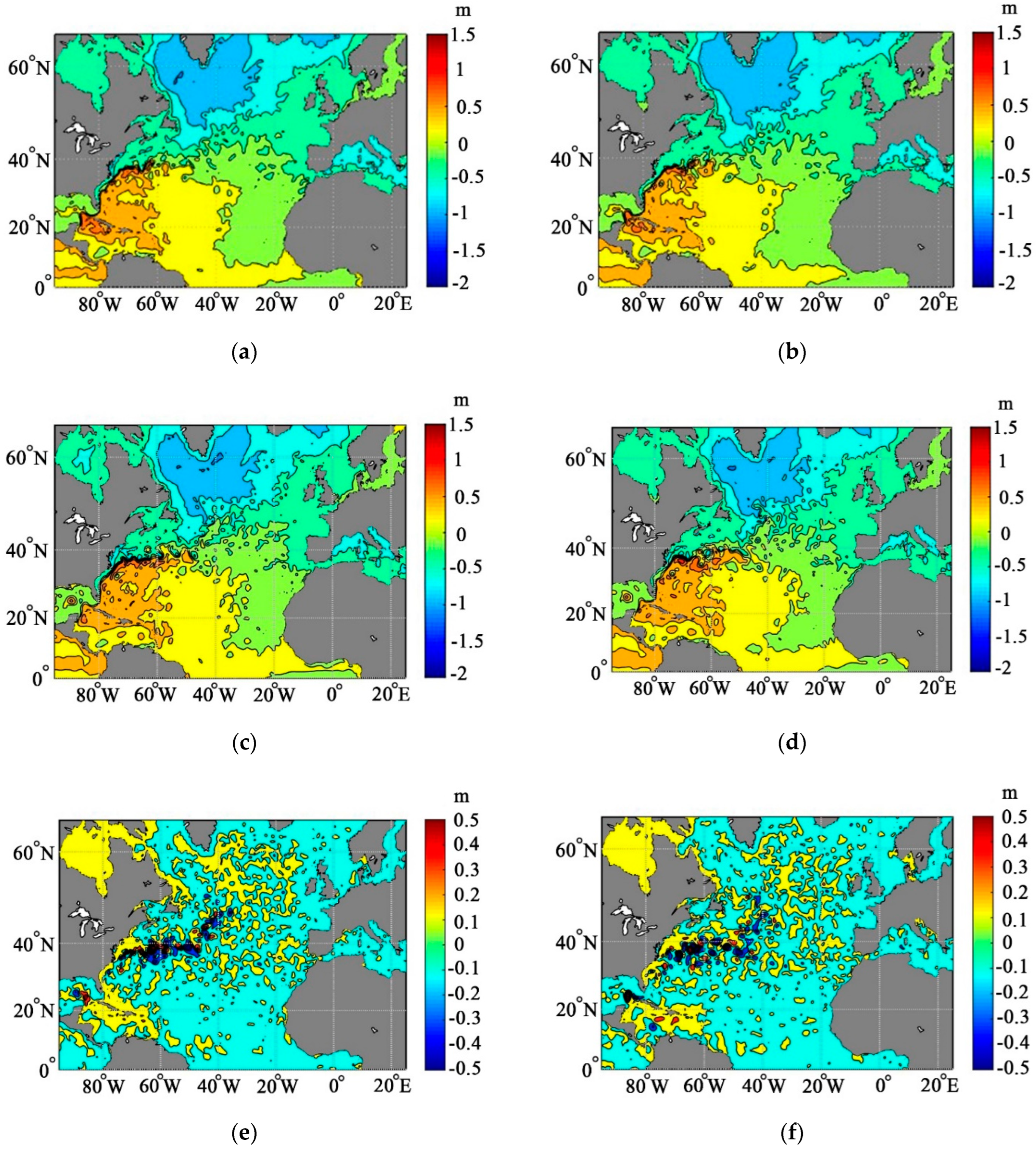
Figure 1 shows the SSH values calculated by the NEMO model without data assimilation (control calculation) (Figure 1a,b), with data assimilation by the GKF method (Figure 1c,d), and their difference (assimilation minus control) (Figure 1e,f) on 8 July and 27 August 2013 for the above-mentioned region of the Atlantic.

It can be seen from Figure 1a,b that the SSH has a pronounced negative large-scale spatial gradient from the south-west to the north-east. A rise of the SSH is distinctly visible in the region of the North Atlantic Current that locally exceeds the SSH to the north of this zone by more than 50 cm.

From the physical point of view, it is evident since this rise of the SSH maintains the current in the direction from the south-west to the north-east and the model describes this tendency correctly. For a one-month period, no global changes occur; a moderate increase in the SSH is seen in the region located to the north of Canada and to the east of the 40° west longitude towards the coast of Africa. One can also notice an increase in the synoptical variability, the occurrence of synoptic eddies both in the Gulf Stream region and to the east of 40° west longitude with a decrease in the SSH by 20–30 cm. Nonetheless, overall, the model demonstrates a fairly regular and smooth change in the SSH with no pronounced bends and eddies. When analyzing the calculation results with data assimilation (Figure 1c,d), the SSH fields become more chaotic and local gradients more pronounced: one can see an increase in the spatial gradient of the SSH between the Gulf Stream region and the cold Labrador Current in the region situated to the west of 60° west longitude; a more vortex field is observed to the north of 40° north latitude. The negative level minimum zone south of Greenland becomes deeper, the minimum values increase and exceed 1 m, while the model calculation shows no such values. In addition, the zone of the negative SSH in the Mediterranean Sea becomes significantly smaller; it is localized closer to the coasts of France and Croatia. However, overall, outside the zone of powerful Atlantic currents, there is no significant difference between the level fields in the calculation with DA and the control calculation. Figure 1e,f show the difference between these fields and their variability for the chosen dates. It can be seen clearly that at the beginning of the calculations with DA, the difference (with the negative sign; i.e., the model value of SSH is higher than the corrected value of SSH) is mainly located within a relatively small region between 35° and 45° north latitude and 40° west longitude, and then, it propagates along the main current of the Gulf Stream and its southern branch and encompasses the zone in the Gulf of Mexico to the south of Florida.

Having said that, the difference itself decreases because, over time, the SSH fields calculated according to the model with DA adjust to the observations. One can see that the initially large positive difference in the Caribbean Sea region decreases significantly, since no powerful current is observed in this region during this period of time. In general, the calculation results both with and without DA demonstrate the adequacy of the used model and the DA method and give appropriate quantitative estimates of the values of SSH fields in the North Atlantic and the adjacent water areas.

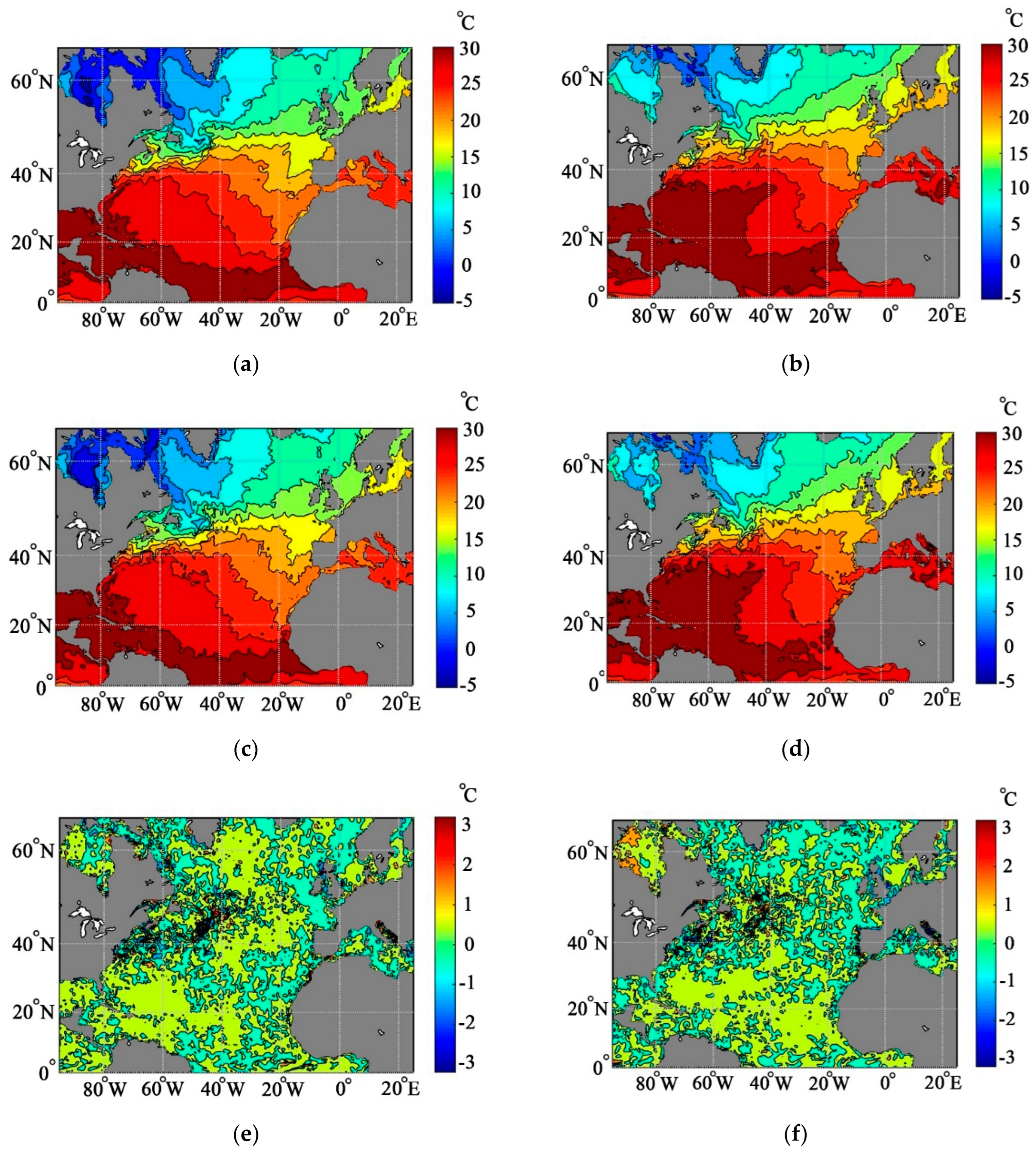
Figure 2 shows the results of calculations of the SST fields by using the NEMO model. Figure 2a,b show variability of the model values of SST with no data assimilation (the control calculation); Figure 2c,d show the SST field calculated with data assimilation according to the GKF method; Figure 2e,f show the difference of the SST fields in the calculation with DA and in the control calculation. It is seen from these figures that the SST fields are consistent with the SSH fields shown in Figure 1; the SST decreases in the direction from the south-west to the north-east, which corresponds to the spatial change in the SSH. That said, the warm SST zone propagates over the two months of calculations from the Gulf of Mexico and the coast of Florida to the middle part of the North Atlantic with a pronounced “tongue” in the direction of the North Atlantic Current up to 38° north latitude and approximately 40° west longitude. The structures of the fields in Figure 1 and Figure 2 are very similar; the difference between the SST fields in Figure 2 is mainly negative and corresponds to the difference between SSH fields shown in Figure 1. However, in comparison with the difference between SSH fields, the difference between SST fields is somewhat shifted to the north, which reflects not only the temperature difference (the thermal shift) but also the dynamics; the shift of the difference between SST fields relative to the difference between SSH fields occurs along the currents. The difference between SST fields decreases with time, just like the difference between SSH fields, since the fields calculated by using the model with DA over time adjust to the observations. At the end of August, a distinct anomalous area appears in the region of the Adriatic Sea near the coasts of Italy and Croatia; the model SST values there clearly exceed the observed SST values.

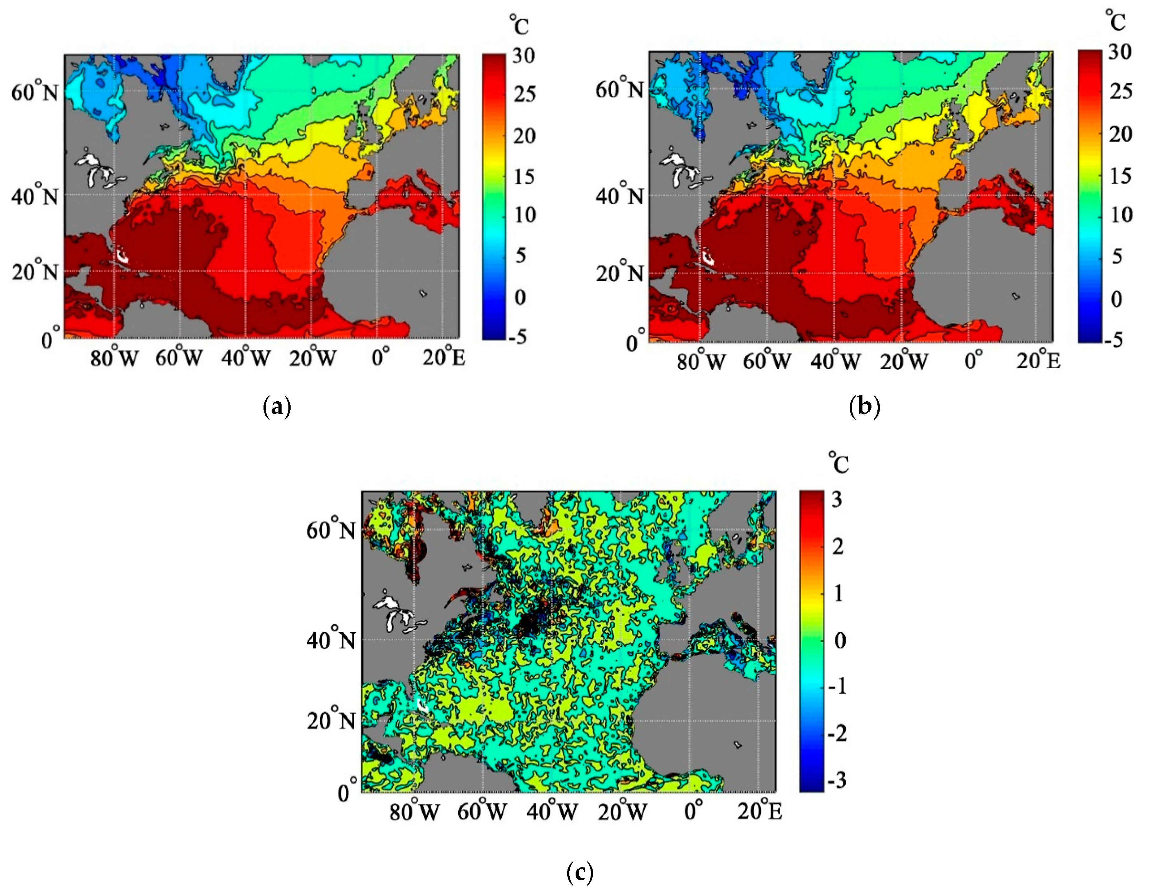
Since the model is three-dimensional, the assimilation of SSH data influences not just the ocean surface temperature but also the subsurface temperature, albeit at relatively shallow depths. Figure 3 shows the behavior of ocean temperature at a depth of 100 m at the halfway date of experiments, namely, on 5 August 2013.

It can be seen that the SST fields in Figure 3a,b are very similar to each other. Some moderate differences are seen in the region near 40° north latitude, with the inflow of warm water in the calculation with no DA as opposed to the calculation with DA. On the contrary, closer to the coast of America, the water in the calculation with DA becomes warmer. It can be seen in the difference between the fields in Figure 3c; however, the values of the difference are small and do not exceed 0.5 °C; they are concentrated both along the US coastline and in the middle part of the North Atlantic, at a point with coordinates 40° north latitude, 40° west longitude. Some difference between the fields is also observed in the Mediterranean Sea, which agrees with the difference between SSHs and the relatively shallow depths both in this region and in the Baltic Sea.

When correcting the model characteristics with the help of the observational data according to the Formulas (2)–(4), the process of information transmission from observational data to the model is performed through the weight matrix K at each time step. The problem of determining this matrix is the key problem in the data assimilation theory. This problem is entirely analogous to the problem of data transmission in radiophysics, where the information transmission from the source to the receiver is performed through the transfer function that is used to transform the amplitude–frequency characteristics of the initial signal. One of the key methods for the analysis of transfer functions in radiophysics is their spectral decomposition (Fourier analysis) which is used to theoretically investigate the properties of the resultant process and also optimize the transceiver devices themselves, filter out the noises, amplify the received signal, etc. Similar problems can be posed in the case of data assimilation. To do so, one must analyze in greater detail the properties of the weight matrix K, determining, in particular, its spectral (amplitude–frequency) characteristics.

As can be seen from the Formulas (4) and (5), the matrix K is the product of the matrices $K_{n+1}=S_{n+1}{Q}_{n+1}^{-1}$, where $S_{n+1}=({\mathsf{\Lambda }}_{n+1}-C_{n+1})(H{\mathsf{\Lambda }}_{n+1}{)}^{\mathrm{T}}$, and the scalar ${\sigma }_{n+1}^2=\left(H{\mathsf{\Lambda }}_{n+1}{)}^{\mathrm{T}}{Q}_{n+1}^{-1}\right(H{\mathsf{\Lambda }}_{n+1})$, whose value in the calculation can be taken to equal 1. The matrix $S_{n+1}$ is defined for all the model variables at each grid point and depends only on the model; the matrix $Q_{n+1}^{-1}$ is the inverse matrix for the covariance matrix of observation error, which depends only on observations and on the already known value of analysis $X_{a,n}$ at the previous time step, which means that in addition to everything else, it is a function of time. Therefore, the structure of the transfer matrix dependent on observations will be determined by the spectral characteristics of matrix $Q_{n+1}^{-1}$ or matrix $Q_{n+1}$, since the eigenvectors of these two matrices coincide, while their eigenvalues are inverse.

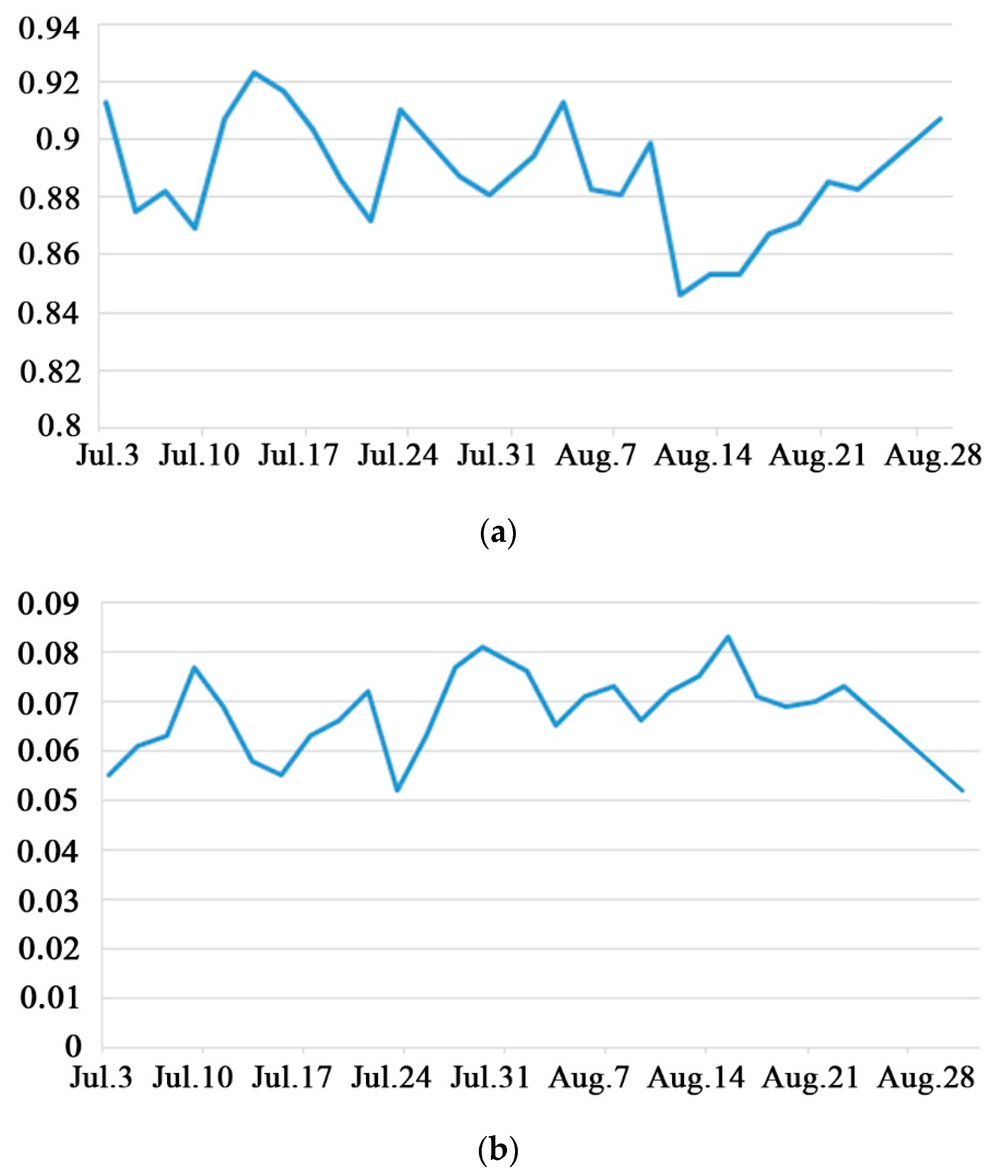
Figure 4 shows the graphs of the first two eigenvalues of the matrix $Q_{n+1}^{-1}$ for n = 1, …, 60. It can be seen that the values of the first eigenvalue (Figure 4a) significantly exceed those of the second eigenvalue (Figure 4b), but the graph of the first eigenvalue has on average a downward trend with a decrease of about 10% for the time interval under review, which can be explained by the model’s “adjusting” to observations over time. In addition, quasi-periodic oscillations of this quantity with a period of about 7–8 days are also observed, which is apparently associated with the astronomical sources of SSH oscillations. The graph of the second eigenvalue has no significant oscillations; its values change within an interval of 0.05–0.08 and there are neither any trends nor a well-pronounced periodicity. It should be noted that the third and subsequent eigenvalues obtained in calculations are small and do not exceed the calculation errors and their graphs are not presented.

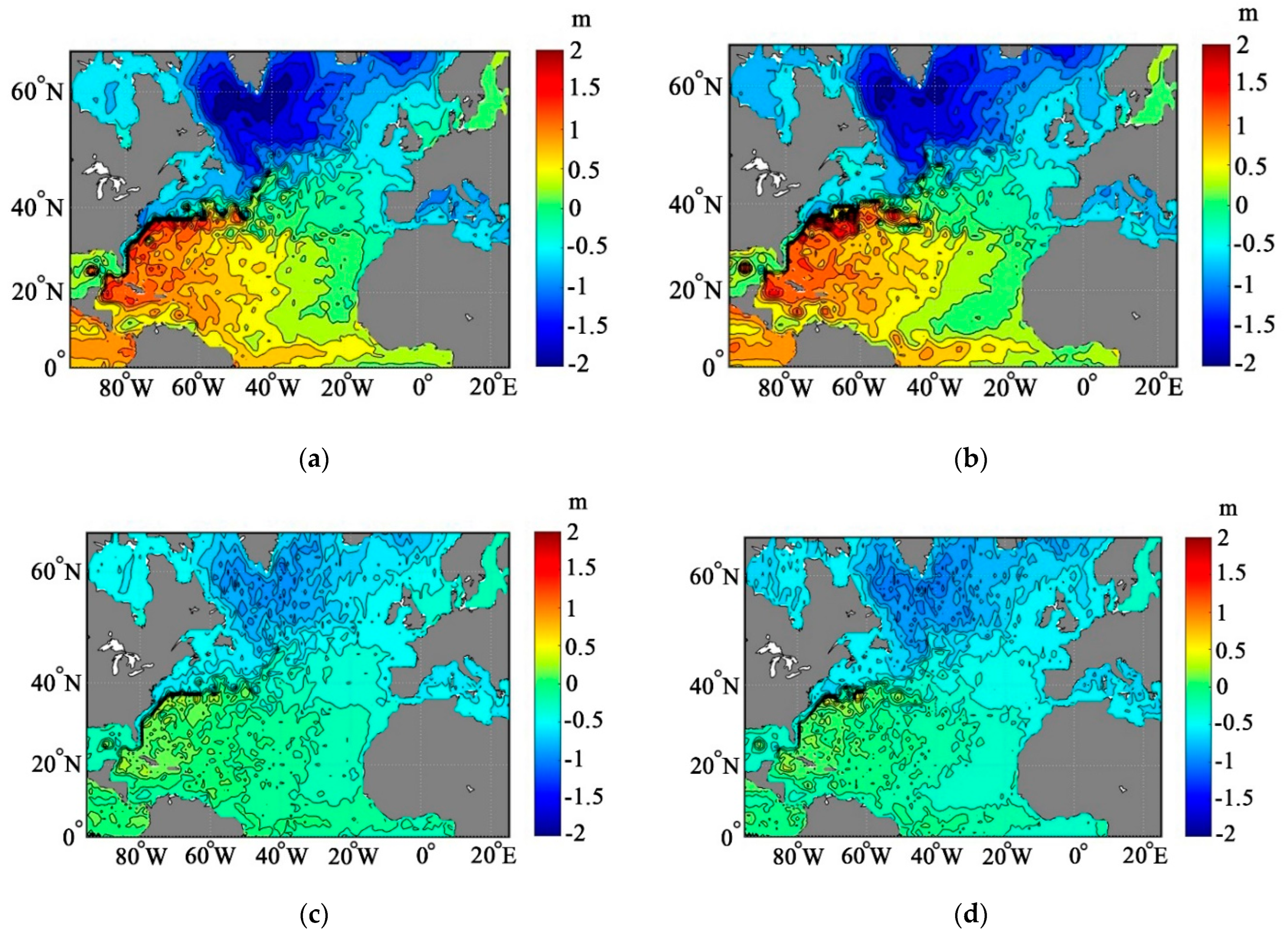
Figure 5 shows the first two eigenvectors of the matrix $Q_{n+1}$ for time moments $t_n$, n = 6, 54, which corresponds to the dates of 5 July 2013 and 25 August 2013. Analyzing the results shown in these figures, we can come to the following conclusions. First, it can be seen that the first eigenvector considerably exceeds the second eigenvector with respect to the values of SSH and spatial gradients of the SSH field. The general direction of the gradients of these fields is the same; a significant decrease with sign inversion occurs in the direction from the south-west to the north-east, which is consistent with the general dynamics of the currents. The gradient is well pronounced in the Gulf Stream region. One can also distinguish the boundary lines in the regions of the Mediterranean Sea–the Atlantic, the Canary Current, and the equatorial currents, as well as other peculiarities of currents in the Atlantic. All these phenomena are present in both figures, meaning that they are typical of both the first and second eigenvectors. Second, the structure of these eigenvectors is very much consistent with the calculated fields with DA and sufficiently consistent with the observations. The general structure of the eigenvectors does not change over time; however, there are some differences in details. For instance, the zone of negative SSH in the regions of the Mediterranean, Adriatic, and Ionic Seas is reduced; the spatial gradient between the Mediterranean Sea and the Atlantic is equalized. The dynamics in the equatorial zone become more pronounced; that said, separate eddies appear in the equatorial current region, which cannot be observed in the figures on the left. The second eigenvector becomes less pronounced; the zone of negative values to the south of Greenland widens but the gradient becomes less pronounced. In general, the dynamics of the eigenvectors is present, but it is not too distinct.

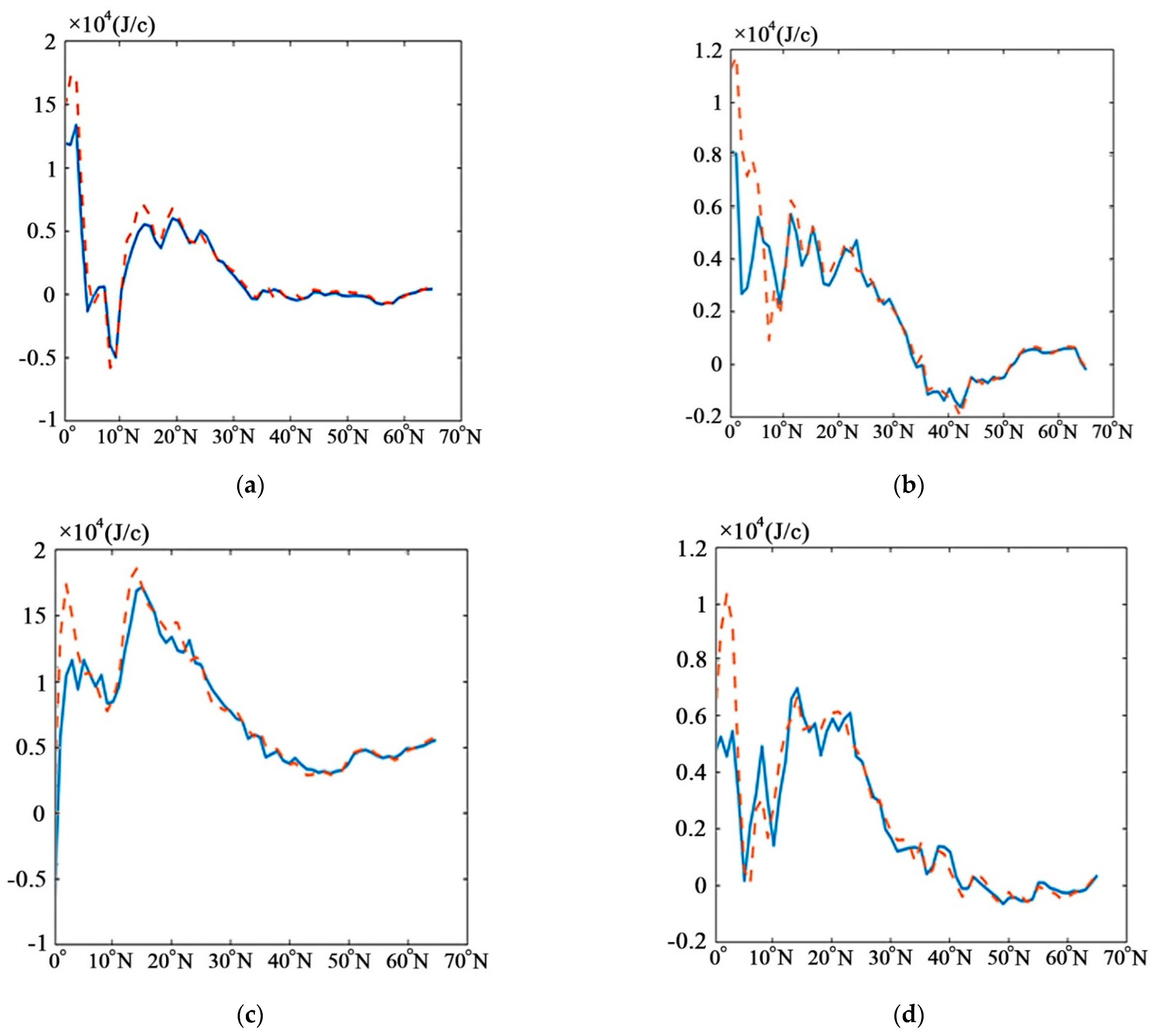
Let us show how certain secondary model characteristics depend on data assimilation. In oceanology and climatology, a very important climate indicator is the meridional heat transfer through a given parallel and its variability over time. Knowing this value, one can estimate the amount of heat transferred from the low to high latitudes and, further, the consumption of this energy in the process of heat transfer from the ocean to the atmosphere, which forms the basis for the medium- and long-term weather and climate forecasts. It goes without saying that in the process of data assimilation, all model characteristics change, including those that determine the meridional heat transfer, namely, the temperature and the meridional component of the currents’ velocity; that said, the changes they exhibit are nonlinear. Therefore, we should expect that the quantitative changes in this characteristic in the process of data assimilation will be much more pronounced than the changes in the SSH, SST, and current velocity.

The meridional heat transfer H (J/c) was calculated by using the formula:

$$H=c_p{\displaystyle \underset{\Sigma }{\iint }\rho Tv\hspace{0.17em}d\sigma },$$

(8)

where $\rho ,T,v$ are the density, temperature, and meridional component of the current velocity, respectively, expressed in the SI units; $c_p$ is the coefficient of water’s heat capacity, which is taken to be 4200 (J/kg °C) in this study. The integral is taken over the area of rectangle Σ, which is the product of the distance along a fixed parallel from the coast of North America to the coasts of Africa or Europe and of the vertical line from the ocean surface to the depth of 200 m.

Figure 6 shows the meridional heat transfer calculated by using Formula (8) for each degree in the North Atlantic. These figures demonstrate that both curves are in close proximity to each other in the regions located to the north of 40° north latitude, where the mainstream of the North Atlantic Current is compensated by the southward current; while discrepancy between these curves becomes quite noticeable to the south of 40° north latitude, where the main branch of the Gulf Stream is especially powerful. That said, it can be seen that while the differences between the control and corrected values of meridional heat transfer were relatively small at the beginning of calculations, by the end of the two-month calculation, the values differ significantly. This fact is explained by the accumulation of such differences in both the velocity fields and the temperature fields. As a consequence, these differences grow over time when integrating the heat flows by using Formula (8).

4. Conclusions

In this work, we present the results of numerical experiments on the calculation of ocean dynamics by using the known NEMO model with the application of the GKF data assimilation method previously developed by the authors. The analysis of the fields of characteristics obtained as a result of modeling with DA is performed by using the method of decomposition into eigenvalues and eigenvectors.

The detailed analysis of variability of both the main model characteristics (sea surface height, temperature, and current fields) and the derived characteristics (heat transfer) has shown that data assimilation has a significant effect. For the main characteristics, the changes in the model fields and in the fields corrected after DA are relatively small (10–15%), although they should not be neglected, especially in some regions. However, for the derived characteristics, such as the heat transfer, the difference is quite pronounced and may reach 30% and more. Therefore, when calculating the long-term variability and heat balance on time intervals of several months and longer, such corrections should be taken into account.

The detailed analysis of the data assimilation process with the help of the decomposition of weight matrices into empirical orthogonal functions (EOFs) shows that the first two orthogonal vectors play the principal role in this decomposition; while their variability over time is rather small, it is noticeable. The first eigenvalue has a distinct average downward trend over a two-month period; the second eigenvalue changes insignificantly. For the SSH field, one can notice the 7- to 8-day variations of these values, which are possibly associated with astronomical sources. In the future, these reasons can be studied in greater detail with the help of correlation and spectral analyses.

In the subsequent works, we plan to perform the assimilation experiments with the NEMO model in conjunction with the GKF method to assimilate not just the SSH data but also the SST and ARGO drift data and to perform assimilation experiments over a longer period of time, lasting up to one year.

References

- Dymnikov, V.P.; Tyrtyshnikov, E.E.; Lykossov, V.N.; Zalesny, V.B. Mathematical modeling of climate, dynamics atmosphere and ocean: To the 95th Anniversary of G.I. Marchuk and the 40th Anniversary of the INM RAS. Izv. Atm. Ocean. Phys. 2020, 56, 215–217. [Google Scholar] [CrossRef]
- Kalman, R.E. A new approach to linear filtering and prediction problems. J. Basic Eng. 1960, 82, 35–45. [Google Scholar] [CrossRef]
- Cummings, J.A.; Smedstad, O.M. Variational data analysis for the global ocean. In Data Assimilation for Atmospheric, Oceanic and Hydrologic Applications; Park, S.K., Xu, L., Eds.; Springer: Berlin/Heidelberg, Germany, 2013; Volume 2, pp. 304–343. [Google Scholar] [CrossRef]
- Agoshkov, V.I.; Ipatova, V.M.; Zalesnyi, V.B.; Parmuzin, E.I.; Shutyaev, V.P. Problems of variational assimilation of observational data for ocean general circulation models and methods for their solution. Izv. Atmos. Ocean. Phys. 2010, 46, 677–712. [Google Scholar] [CrossRef]
- Carrassi, A.; Bocquet, M.; Bertino, L.; Evensen, G. Data assimilation in the geosciences: An overview of methods, issues, and perspectives. WIREs Clim. Chang. 2018, 9, e535. [Google Scholar] [CrossRef]
- Kalnay, E.; Ota, Y.; Miyoshi, T.; Liu, J. A simpler formulation of forecast sensitivity to observations: Application to ensemble Kalman filters. Tellus A 2012, 64, 18462. [Google Scholar] [CrossRef]
- Barker, D.; Lorenc, A.; Clayton, A. Hybrid Variational/Ensemble Data Assimilation. ECMWF Data Assimilation Seminar, 6 September 2011. Crown Copyright 2011. Source: Met Office. Available online: https://www.ecmwf.int/sites/default/files/elibrary/2011/14950-hybrid-variationalensemble-data-assimilation.pdf (accessed on 18 May 2023).
- Bell, M.J.; Lefèbvre, M.; Le Traon, P.-Y.; Smith, N.; Wilmer-Becker, K. GODAE: The Global Ocean data assimilation experiment. Oceanography 2009, 22, 14–21. [Google Scholar] [CrossRef]
- Tanajura, C.A.S.; Santana, A.N.; Mignac, D.; Lima, L.N.; Belyaev, K.P. Observing system experiments over the Atlantic Ocean with the REMO ocean data assimilation system (RODAS) into HYCOM. Ocean Dyn. 2020, 70, 115–138. [Google Scholar] [CrossRef]
- Oke, P.R.; Brassington, G.B.; Griffin, D.A.; Schiller, A. The Bluelink Ocean Data Assimilation System (BODAS). Ocean Model. 2007, 21, 46–70. [Google Scholar] [CrossRef]
- Cummings, J.; Smedstad, M. Ocean Data Impacts in Global HYCOM. J. Atm. Ocean. Technol. 2014, 31, 1771–1791. [Google Scholar] [CrossRef]
- Tanajura, C.A.S.; Belyaev, K. A sequential data assimilation method based on the properties of a diffusion-type process. Appl. Math. Mod. 2009, 33, 2165–2174. [Google Scholar] [CrossRef]
- Belyaev, K.; Kuleshov, A.; Tuchkova, N.; Tanajura, C.A.S. An optimal data assimilation method and its application to the numerical simulation of the ocean dynamics. Math. Comput. Model. Dyn. Syst. 2018, 24, 12–25. [Google Scholar] [CrossRef]
- Belyaev, K.P.; Kuleshov, A.A.; Smirnov, I.N.; Tanajura, C.A.S. Generalized Kalman Filter and Ensemble Optimal Interpolation, their comparison and application to the Hybrid Coordinate Ocean Model. Mathematics 2021, 9, 2371. [Google Scholar] [CrossRef]
- Bleck, R.; Boudra, D. Initial testing of a numerical ocean circulation model using a hybrid (quasi-isopycnic) vertical coordinate. J. Phys. Oceanogr. 1981, 11, 755–770. [Google Scholar] [CrossRef]
- Gusev, A.; Diansky, N. Numerical simulation of the world ocean circulation and its climatic variability for 1948–2007 using the INMOM. Izvestiya Atm. Ocean. Phys. 2014, 50, 1–12. [Google Scholar] [CrossRef]
- Madec, G.; The NEMO team. NEMO ocean engine. Note du Pole de modélisation de l’Institut Pierre-Simon Laplace. 2016, 27. NEMO ocean engine. Available online: nemo-ocean.eu (accessed on 18 May 2023).
- Dussin, R.; Barnier, B.; Brodeau, L. DRAKKAR/MyOcean; Report 01-04-16; LGGE: Grenoble, France, 2016; Available online: https://www.drakkar-ocean.eu/publications/reports/report_DFS5v3_April2016.pdf (accessed on 18 May 2023).
- Belyaev, K.; Kuleshov, A.; Smirnov, I. Spatial–temporal variability of the calculated characteristics of the ocean in the Arctic zone of Russia by using the NEMO model with altimetry data assimilation. J. Mar. Sci. Eng. 2020, 8, 753. [Google Scholar] [CrossRef]
- Belyaev, K.; Tanajura, C.A.S. An extension of a data assimilation method based on the application of the Fokker–Planck equation. Appl. Math. Model. 2002, 26, 1019–1027. [Google Scholar] [CrossRef]
- Belyaev, K.P.; Kuleshov, A.A.; Tuchkova, N.P. The stability problem for a dynamic system with the assimilation of observational data. Lobachevskii J. Math. 2019, 40, 911–917. [Google Scholar] [CrossRef]
- Belyaev, K.; Kuleshov, A.; Smirnov, I. Spatial decomposition of covariance functions in Generalized Kalman filter method for data assimilation. In Proceedings of the 2020 Ivannikov Ispras Open Conference (ISPRAS), Moscow, Russia, 10–11 December 2020; pp. 125–129. [Google Scholar] [CrossRef]
- Schmidt, O.T.; Mengaldo, G.; Balsamo, G.; Wedi, N.P. Spectral empirical orthogonal function analysis of weather and climate data. Mon. Weather. Rev. 2019, 147, 2979–2995. [Google Scholar] [CrossRef]
- Shapiro, G.I.; Gonzalez-Ondina, J.M. An efficient method for nested high-resolution ocean modelling incorporating a data assimilation technique. J. Mar. Sci. Eng. 2022, 10, 432. [Google Scholar] [CrossRef]
- Timkoa, P.G.; Arbicb, B.K.; Hyderd, P.; Richmane, J.G.; Zamudioe, L.; O’Dead, E.; Wallcrafte, A.J.; Shriverf, J.F. Assessment of shelf sea tides and tidal mixing fronts in a global ocean model. Ocean. Model. 2019, 136, 66–84. [Google Scholar] [CrossRef]
- UNESCO Formula. Available online: https://link.springer.com/content/pdf/bbm%3A978-3-319-18908-6%2F1.pdf (accessed on 29 January 2023).
- AVISO Satellite Altimetry Data. Available online: http://www.aviso.altimetry.fr (accessed on 29 January 2023).
- Hybrid Computer K-60. Available online: http://www.kiam.ru/MVS/resourses/k60.html (accessed on 29 January 2023).
Figure 1.
Sea surface height field (m) calculated by using the NEMO model on 8 July (on the left) and 27 August (on the right), 2013: (a,b) calculation with no DA (the control calculation), (c,d) calculation with DA by the GKF method, and (e,f) difference between SSHs in calculations with and without DA.
Figure 2.
The sea surface temperature (SST) fields (°C) calculated by using the NEMO model on 8 July (on the left) and 27 August (on the right), 2013: (a,b) calculation with no DA (the control calculation), (c,d) calculation with DA by the GKF method, and (e,f) difference between SSTs in calculations with and without DA.
Figure 3.
The sea temperature fields (°C) at a depth of 100 m calculated by using the NEMO model on 5 August 2013: (a) with no DA (the control calculation), (b) with DA by the GKF method, and (c) difference between the SST fields in calculations with and without DA.
Figure 4.
Two first eigenvalues of the matrix calculated by using the NEMO model with DA by the GKF method: (a) first eigenvalue and (b) second eigenvalue.
Figure 5.
Maps of the two first eigenvectors (m) of the matrix calculated by using the NEMO model with DA by the GKF method on 5 July (on the left) and 25 August (on the right), 2013: (a,b) first eigenvector and (c,d) second eigenvector.
Figure 6.
North Atlantic meridional heat transfer (J/c) calculated by using the NEMO model; the blue curve refers to the calculation without DA (the control) and the red dotted curve refers to the calculation with DA by the GKF method: (a) on 5 July 2013, (b) on 5 August 2013, (c) on 15 August 2013, and (d) on 25 August 2013.
Disclaimer/Publisher’s Note: The statements, opinions and data contained in all publications are solely those of the individual author(s) and contributor(s) and not of MDPI and/or the editor(s). MDPI and/or the editor(s) disclaim responsibility for any injury to people or property resulting from any ideas, methods, instructions or products referred to in the content. |
© 2023 by the authors. Licensee MDPI, Basel, Switzerland. This article is an open access article distributed under the terms and conditions of the Creative Commons Attribution (CC BY) license (https://creativecommons.org/licenses/by/4.0/).
Share and Cite
MDPI and ACS Style
Belyaev, K.; Kuleshov, A.; Smirnov, I. Analysis of the Model Characteristics in the North Atlantic Simulated by the NEMO Model with Data Assimilation. J. Mar. Sci. Eng. 2023, 11, 1078. https://doi.org/10.3390/jmse11051078
AMA Style
Belyaev K, Kuleshov A, Smirnov I. Analysis of the Model Characteristics in the North Atlantic Simulated by the NEMO Model with Data Assimilation. Journal of Marine Science and Engineering. 2023; 11(5):1078. https://doi.org/10.3390/jmse11051078
Chicago/Turabian StyleBelyaev, Konstantin, Andrey Kuleshov, and Ilya Smirnov. 2023. "Analysis of the Model Characteristics in the North Atlantic Simulated by the NEMO Model with Data Assimilation" Journal of Marine Science and Engineering 11, no. 5: 1078. https://doi.org/10.3390/jmse11051078
Note that from the first issue of 2016, this journal uses article numbers instead of page numbers. See further details here.