Article

Application of Idealised Modelling and Data Analysis for Assessing the Compounding Effects of Sea Level Rise and Altered Riverine Inflows on Estuarine Tidal Dynamics

1
Water Research Laboratory, School of Civil and Environmental Engineering, UNSW Sydney, Sydney, NSW 2093, Australia
2
University Rouen Normandie, UNICAEN, CNRS, M2C UMR 6143, F-76000 Rouen, France
*
Author to whom correspondence should be addressed.
J. Mar. Sci. Eng. 2023, 11(4), 815; https://doi.org/10.3390/jmse11040815
Submission received: 24 February 2023 / Revised: 24 March 2023 / Accepted: 6 April 2023 / Published: 11 April 2023
(This article belongs to the Special Issue Estuaries, Coasts, and Seas in a Changing Climate)

Abstract

:
Estuaries worldwide are experiencing increasing threats from climate change, particularly from the compounding effects of sea level rise (SLR) and varying magnitude of river inflows. Understanding the tidal response of estuaries to these effects can guide future management and help assess ecological concerns. However, there is limited existing understanding on how estuarine tidal dynamics may respond to the compounding effects of SLR and altered riverine inflows in different estuaries. To partially address this knowledge gap, this study used data analysis and scrutinised idealised hydrodynamic models of different estuary shapes and boundary conditions to (i) identify broad effects of SLR on estuarine tidal dynamics under various river inflow conditions, (ii) determine how longitudinal cross-sections are impacted by these effects, and (iii) highlight some implications for environmental risk management. Results indicated that short- to moderate-length, high convergent estuaries experience the greatest and short- to moderate-length prismatic and low convergent estuaries experience the least variations in their overall tidal dynamics (i.e., tidal range, current velocity, and asymmetry). These variations were most evident in estuaries with large riverine inflows and macrotidal conditions. Compounding effects of SLR and altered riverine inflows induced spatially heterogenous changes to tidal range, current velocity, and asymmetry, with transects nearest to the estuary mouth/head and at a three-quarter estuary length (measured from estuary mouth) identified as the most and the least vulnerable zones, respectively. These findings provide an initial broad assessment of some effects of climate change in estuaries and may help to prioritise future investigations.

1. Introduction

Estuaries are amongst the most populated regions worldwide and are important locations for economic, cultural, and recreational activities. Estuaries offer a range of ecosystem services to humans including (but not limited to) water purification, food provision, and flood/erosion protection [1,2,3]. There is widespread consensus that climate change impacts, especially the compounding effects of sea level rise (SLR) and altered riverine inflows, increasingly endanger these ecosystem services and threaten the livelihoods of millions of people inhabiting estuarine environments [4,5,6,7].
SLR and altered riverine inflows (as well as their compounding effects) can alter estuarine tidal dynamics and potentially lead to erosion, entrance instability, failure of drainage systems, more frequent inundation, saltwater intrusion, and the loss of wetlands and associated ecosystems [8,9,10,11,12,13,14]. The variations in the magnitude of river inflows (hereafter called varying river inflows or altered riverine inflows) can alter estuarine tidal dynamics (e.g., tidal range) by changing the surface water slope and influencing the effective roughness and energy dissipation [15,16,17]. SLR has been observed to change the tidal prism, water depth, frictional effects, and the location of nodal points, modifying the tidal structure and propagation patterns [17,18,19]. Depending on the estuarine form (or geomorphic typology), tidal modifications induced by SLR and/or altered riverine inflows may deteriorate water quality, threaten vegetation communities, and alter the sediment budget and geomorphology over time and space [17,18,19]. As such, research that furthers the understanding of estuarine tidal dynamics is important as it may assist in guiding future assessments and management efforts.
Idealised hydrodynamic approaches (i.e., using simplified estuarine geometries such as converging and prismatic channels and running an ensemble of scenarios) have been identified as a promising approach to predict changes in estuarine tidal dynamics [20,21,22,23,24,25]. Idealised models require reduced data collection and computational resources compared with full hydrodynamic approaches and have been found to provide reasonable agreement with theoretical, analytical, and process-based assessments of estuarine hydrodynamics at real-world sites [20,21,22,26]. For instance, idealised prismatic and converging models of estuaries were observed to replicate tidal range responses obtained from a process-based model for the Chesapeake Bay and its tributaries such as the Potomac River, Rappahannock River, and York River [20], as well as the tidal range values obtained from analytical approximations [26]. However, idealised models typically include a large number of simulations to assess variations in estuary hydrodynamics due to the vast array of estuarine parameters, including shapes (e.g., length, depth, and convergence) and boundary conditions (e.g., friction) [21,22].
When dealing with idealised models, researchers have previously investigated individual tidal properties (e.g., tidal range)—as opposed to overall assessments of tidal properties (e.g., changes in tidal range, currents, and asymmetry)—under different boundary conditions and compounding effects [20,21,27,28,29]. Considering the quantity of hydrodynamic properties, the application of generic data analysis techniques may provide a promising approach to analyse large datasets and has been successfully applied to hydrodynamic and hydrology disciplines [30,31,32]. For instance, data analysis methods (e.g., neural network and random forest) have been utilised to assess flood risks [33,34,35,36], boundary condition enhancement [37], water quality [38,39], and spatial distribution of mobile organisms (e.g., fish) [40,41] in different water bodies worldwide.
As such, this study examines the application of a generic data analysis method to a large dataset of idealised models with findings specifically focusing on the compounding effects of SLR and altered riverine inflows. In particular, this study used a Pearson correlation analysis to explore the tidal dynamics (herein, simply defined as changes in tidal range, current velocity, and asymmetry) of a set of idealised hydrodynamic models with different estuary shapes (i.e., prismatic and converging) and boundary conditions (e.g., bed/banks friction) in present-day conditions and under future SLR, varying river inflows, and compounding conditions. Throughout this article, the overarching changes to tidal properties (i.e., tidal range, current velocity, and asymmetry) due to the effects of SLR and/or altered riverine inflows for different estuaries are discussed. Where relevant, findings are compared with real-world sites to cross-check the practicality of their application. Overall, this study addresses the following scientific questions:
  • Are data analysis techniques able to provide broad insights into the effects of SLR and varying river inflows on estuarine tidal dynamics?
  • What are the dominant effects of SLR and altered riverine inflows on estuarine tidal properties?
  • Which estuary types and locations are most vulnerable to changes in mean sea level and river inflows?
This paper is structured as follows. Section 2 presents the methodology, simulations, and tidal properties considered, as well as the data analysis techniques adopted. Section 3 details how parameters representative of estuarine tidal dynamics including tidal range, maximum current velocity, and asymmetry are likely to alter under the compounding influence of SLR and altered riverine inflows. Finally, Section 4 elaborates on the implications of altered tidal dynamics for estuarine management, provides broad conclusions, and offers directions for future research efforts.

2. Methods

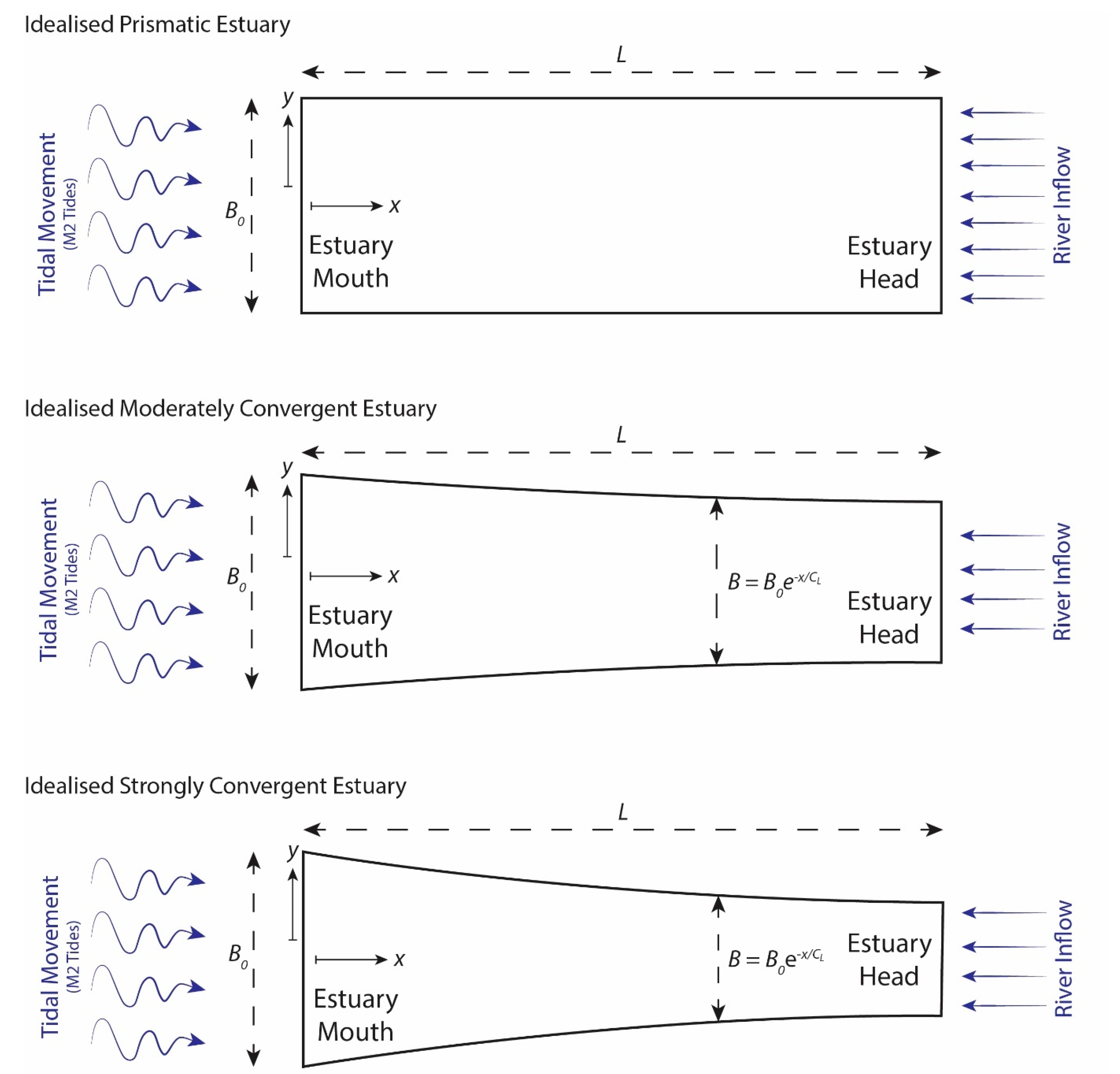
2.1. Numerical Modelling

A large subset of idealised simulations conducted by [21] has been re-analysed in this research. These simulations considered three simplified geometries comprising prismatic estuaries and converging estuaries with convergence lengths of CL = 160 km (weaker convergence) and CL = 80 km (stronger convergence) (Figure 1). Combinations of a wide range of estuarine parameters were investigated comprising estuary length (L = 40, 80, and 160 km), uniformly distributed Manning’s roughness (n = 0.015 and 0.03 s/m1/3), tidal range at the mouth (TR0 = 0.5, 1, and 4 m, representing microtidal, mesotidal, and lower boundaries of macrotidal coastal conditions, respectively), river inflow (Q) over tidal prism (TP) ratio (Q/TP = 0%, 1%, 5%, and 10%), and SLR = 0 and 1 m. The width at the mouth (B0 = 1000 m) and water depth (h = 5 m) were kept constant, and for all cases, sinusoidal M2 tides (as the dominant semi-diurnal tidal constituent along the majority of coastlines and a proxy for tidal range) were applied at the mouth with a period of T = 12.42 h. Initially, no river inflow was considered (Q/TP = 0%) to identify the tidal prism TP (i.e., the volume of water entering an estuary over a flood cycle). Using the identified TP, constant river inflows (Q/TP = 1%, 5%, and 10%) were adopted. The range of considered river inflow represents low to high fluvial input conditions. The combination of all variables resulted in 432 simulation cases (144 simulations for each estuary geometry).
The RMA-2 modelling package was used for the hydrodynamic modelling, which solves depth- and Reynolds-averaged Navier–Stokes equations using a finite element method [42]. To define the turbulent characteristics, the model utilises horizontal eddy viscosity coefficients [43]. The model captures the flow field, velocity components in the horizontal plane, and water surface elevations. Further details regarding the modelling suite, implementation of boundary conditions, model accuracy, and grid independence have been presented in previous research [21,22,44].

2.2. Tidal Properties
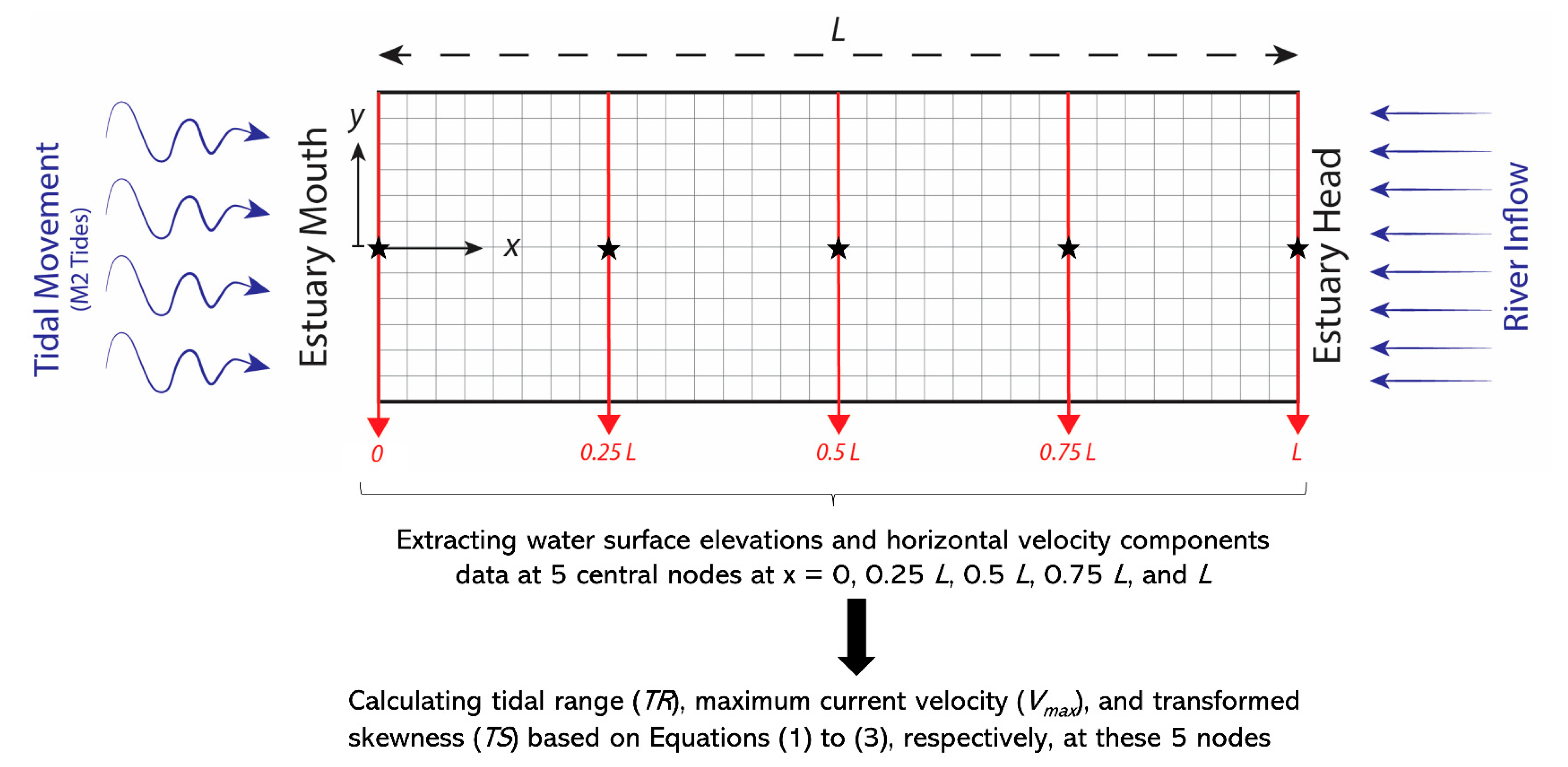
To achieve the research objectives, three key tidal properties that provide insights into inundation, shoreline recession, failure of drainage systems, etc. were extracted along the central nodes for each of the investigated cases including tidal range, maximum current velocity, and tidal asymmetry. In this study, tidal range (TR) is defined as the difference in the maximum water height during high tide ( δ ¯ h i g h ) and the minimum water height during low tide ( δ ¯ l o w ) measured along the central nodes of the estuaries:
T R = δ ¯ h i g h δ ¯ l o w
The maximum current velocity ( V m a x ) is calculated as the maximum of total current speed as resulting from maximum horizontal speeds at the x ( V x ,   m a x ) and y ( V y ,   m a x ) directions (see Figure 1) along the central nodes:
V m a x = V x ,   m a x 2 + V y ,   m a x 2
The tidal asymmetry, a tidal wave deformation process highlighting the inequality of the duration of rise and fall of tidal levels, can be characterised using statistical measures. Here transformed skewness (TS), as an asymmetry proxy, is used and can be calculated as
T S = S k i m a g H i η
S k x = 1 L t 1 t = 1 L t η t η ¯ 3 1 L t 1 t = 1 L t η t η ¯ 2 3 / 2
where Sk() is the skewness indicator, imag() represents the imaginary part, Hi() indicates the Hilbert transform, η t is the input signal time series, η ¯ is the mean value, and Lt is the length of equidistant time series data [45]. A positive value of TS denotes a longer rising tide duration and an ebb-dominated system, whereas a negative value suggests a longer falling tide duration and a flood-dominated system [45].

2.3. Data Analysis

For all 432 cases, these properties were evaluated at central nodes along the estuary (Figure 2), producing a large database of tidal properties. For this database, after an initial cluster analysis was conducted (for details, see [46]), a Pearson correlation (α) analysis was performed to identify changes induced by 1 m of SLR and varying river inflows (Q/TP = 0%, 1%, 5%, and 10%) on TR, V m a x , and TS. These results were extracted at five nodes along the estuaries comprising x = 0 (mouth), 0.25 L, 0.5 L, 0.75 L, and L (estuary head) (Figure 2). Note that an offset of 2 km was applied at the mouth and the estuary head to eliminate outliers in the dataset due to model effects. Although the Pearson correlation analysis denotes a simplified, linear association between two variables, it is a reasonable choice in providing empirical, first-pass estimates of changes in tidal properties [22].
Results from the Pearson correlation provided coefficients between −1 ≤ α ≤ +1, representing the linear association between two variables (e.g., tidal range and SLR), where a change in one variable is accompanied with a consistent change in the second variable. A value of α = −1 indicated a negative correlation, α = 0 indicated no correlation, and α = +1 indicated a positive correlation. A value of 0 α < 0.3 is commonly considered as a very weak correlation, 0.3   α < 0.5 is considered a weak correlation, 0.5 α < 0.7 is considered a moderate correlation, and 0.7 α 1 is considered a strong correlation. In this study, correlations that are very weak or weak were combined (0 α 0.5) and considered as “weak”, whereas moderate or strong correlations were regarded as “strong” (0.5 < α 1).

3. Results

This section presents the results of the Pearson correlation analysis to identify the influence of SLR and/or river inflows on tidal range (Table 1), maximum current velocity (Table 2), and transformed skewness (Table 3). The importance of estuary geometry (i.e., shape and length) and frictional effects as well as microtidal, mesotidal, and macrotidal coasts in assessing estuarine tidal dynamics under SLR and altered river inflow effects is also discussed. The results of these three representative tidal parameters were analysed for five different central nodes along the estuaries (x = 0, 0.25 L, 0.5 L, 0.75 L, and L; see Figure 2), which are represented by five consecutive triangles in the cells of Table 1, Table 2 and Table 3. For each river inflow scenario (Q/TP = 0% representing no inflows, Q/TP = 1% representing low inflows, Q/TP = 5% representing moderate inflows, and Q/TP = 10% representing high inflows), upward and downward directed triangles depict an increase or a decrease in any given tidal property due to 1 m of SLR. Hollow and solid triangles denote weak and strong Pearson correlations, respectively. To easily locate each cell in Table 1, Table 2 and Table 3, 2D indices are introduced such that rows are numbered from “1” to “36”, and columns are marked by the letters “a” to “f”. As such, when presenting the results, any given cell is referred to with a letter-number index. Further, dominant patterns of change in tidal range, maximum current velocity, and transformed skewness along the estuaries are highlighted with the same cell colour (e.g., shade of green, blue, or red) across Table 1, Table 2 and Table 3. This shading facilitates a cross-comparison between tidal properties and the overarching trends.

3.1. Effects of SLR and/or Altered Riverine Inflows on Estuarine Tidal Range

Table 1 summarises the effects that SLR and/or riverine inflows can have on the tidal range along the estuaries. Two general patterns of change in tidal range were found:
(i)
SLR led to minor (weak) increases in tidal range along the estuaries (dark green coloured cells);
(ii)
SLR substantially increased the tidal range at the mouth and then minimally strengthened it in a landward direction (light green coloured cells).
The first pattern dominated in prismatic and converging estuaries with microtidal or mesotidal coastal conditions (TR0 = 0.5 and 1 m), while the second pattern was often observed in estuaries with macrotidal conditions (TR0 = 4 m). Where SLR increased the tidal range, this was consistent with reported research of real-world estuaries, such as the Elbe River [47], York River [20], Rappahannock River [20], Hudson–Raritan Estuary [48], and Minnamurra River [49]. In these cases, amplified tides may exceed the crest of protective structures, exacerbate flood events [50], and lead to the failure of surface drainage infrastructures; shoreline erosion; and loss of wetlands, intertidal areas, and their associated ecosystems [7,12,51].
Converging estuaries were likely to amplify the tidal range under compounding effects of high inflows and high initial tidal range (Table 1). For all estuary shapes, and under these compounding conditions, SLR always amplified (often strongly) the tidal range at the estuary mouth. Interestingly, the tidal range for prismatic and converging estuaries with CL = 160 km largely varied along the first half of the estuary length (i.e., 0  x 0.5 L), whereas areas of strong tidal variations were located around the mouth and head (i.e., x = 0 and L) of converging estuaries with CL = 80 km. This finding aligned with predictions in real-world estuaries, such as the moderately converging Patuxent Estuary (L = ~40 km), which may experience larger variations in tidal range in its first 20 km [20], and the strongly converging Delaware Bay estuary, which may undergo a substantial tidal amplification in its upstream zones [52].
Tidal range also varied dynamically and nonlinearly under SLR for estuaries with high initial tidal range (TR0 = 4 m) (Table 1). In these estuaries, the dampening effect of the bottom friction became important (particularly in the upstream part of the estuary), and a larger Manning’s n could lead to a weaker tidal range amplification. For instance, in a converging estuary with CL = 80 km, TR0 = 4 m, L = 40 km, and Q/TP = 10%, a substantial increase in tidal range with an SLR of 1 m was observed at x = 0, 0.5 L, and L for n = 0.015 s/m1/3, whereas for n = 0.03 s/m1/3, the tidal range only increased at x = 0 (cells a-36 and b-36 in Table 1). In this case, it appeared that the convergence effect outweighed the reduced frictional effects under SLR when n = 0.015 s/m1/3, but friction dominated when Manning’s n increased to n = 0.03 s/m1/3. There were only four cases with CL = 80 km, L = 40 and 80 km, n = 0.015 and 0.03 s/m1/3, and Q/TP = 5% and 10% (cells a-35, b-35, c-35, and a-36 in Table 1) that experienced a substantial increase in tidal range at three or more nodes along the estuary when SLR = 1 m. Such an increase in tidal range due to SLR was observed in several estuaries around the British coast such as the Severn Estuary, which is a converging macrotidal site [53].
Effects of variations in inflows and the compounding effects with SLR are also shown in Table 1. Inflow effects on the tidal range patterns were predominantly evident in estuaries with either a high tidal range at the mouth (TR0 = 4 m) or a strongly converging shape (CL = 80 km) (Table 1). For example, in a converging estuary with CL = 160 km, TR0 = 4 m, L = 160 km, and n = 0.015 s/m1/3, an SLR of 1 m caused a tidal range amplification at all transects when Q/TP = 1%, with the strongest increases observed at the mouth (cell e-22 in Table 1). However, when Q/TP = 5%, SLR only strongly intensified the tidal range at the mouth, with tidal attenuation observed at x = 0.75 L (cell e-23 in Table 1). Increasing inflows appeared to act against the tidal propagation leading to tidal attenuation in the upstream part of the estuary [54]. A similar trend under rising river inflows has been reported in real-world estuaries, including the Ganges–Brahmaputra–Meghna Delta [55], the Scheldt Estuary [56], and the Pearl River [57].
There were a few cases (mainly prismatic or converging with CL = 160 km estuaries) where SLR could reduce the tidal range. These mainly included transects (nodes) at x = 0.25 L for prismatic cases with TR0 = 0.5 and 1 m, L = 160 km, n = 0.015 and 0.03 s/m1/3, and Q/TP = 0% and 1% (cells e-1, f-1, e-2, f-2, e-5, f-5, e-6, and f-6 in Table 1); transects at 0.25 Lx ≤ 0.5 L for prismatic cases with TR0 = 4 m, L = 40 and 80 km, n = 0.015 s/m1/3, and Q/TP = 5% (cells a-11 and c-11 in Table 1); and transects at x = 0.75 L for converging estuaries with CL = 160 km, TR0 = 4 m, L = 40, 80, and 160 km, n = 0.015 and 0.03 s/m1/3, and Q/TP = 1% and 5% (cells a-22 to e-22 and a-23 to f-23 in Table 1).
Table 1. Compounding effects of SLR and varying river inflows on tidal range at five nodes along the estuaries (x = 0, 0.25 L, 0.5 L, 0.75 L, and L), which are represented by five consecutive triangles in each cell. Upward and downward triangles indicate an increase or a decrease in tidal range induced by 1 m of SLR and for four varying river inflows (Q/TP = 0%, 1%, 5%, and 10%). Hollow and solid triangles imply weak (0 α 0.5) and strong (0.5 < α 1) Pearson correlation coefficients, respectively. The symbol “–” denotes the absence of a correlation (for details, see [46]). Dominant patterns of change in tidal properties under compounding effects of SLR and river inflows are highlighted with similar colours across Table 1, Table 2 and Table 3.
abcdef
L40 km80 km160 km
n0.015 s/m1/30.03 s/m1/30.015 s/m1/30.03 s/m1/30.015 s/m1/30.03 s/m1/3
PrismaticTR0 = 0.5 mNo inflow (Q/TP = 0%)
△△△△△△△△△△△△△△△△△△△△△▽△△△△▽△△△1
Low inflow (Q/TP = 1%)
△△△△△△△△△△△△△△△△△△△△△▽△△△△▽△△△2
Moderate inflow (Q/TP = 5%)
△△△△△△△△△△△△△△△△△△△△△△△△△△△△△△3
High inflow (Q/TP = 10%)
△△△△△△△△△△△△△△△△△△△△△△△△△△△△△△4
TR0 = 1 mNo inflow (Q/TP = 0%)
△△△△△△△△△△△△△△△△△△△△△▽△△△△▽△△△5
Low inflow (Q/TP = 1%)
△△△△△△△△△△△△△△△△△△△△△▽△△△△▽△△△6
Moderate inflow (Q/TP = 5%)
△△△△△△△△△△△△△△△△△△△△△△△△△△△△△△7
High inflow (Q/TP = 10%)
△△△△△△△△△△△△△△△△△△△△△△△△△△△△△△8
TR0 = 4 mNo inflow (Q/TP = 0%)
△△△△△△△△△△△▲△△△△△–△△△△△△△△△△△△9
Low inflow (Q/TP = 1%)
▲△△△△▲△△△△▲△△△△▲△–△△▲△△△△▲△△△△10
Moderate inflow (Q/TP = 5%)
▲▽▽△△▲△–△△▲▽▽△△▲△△△△▲△△△△▲△△△△11
High inflow (Q/TP = 10%)
▲△△△△▲△△△△▲△△△△▲△△△△▲△▲△△▲△△△△12
Converging with CL = 160 kmTR0 = 0.5 mNo inflow (Q/TP = 0%)
△△△△△△△△△△△△△△△△△△△△△△△△△△△△△△13
Low inflow (Q/TP = 1%)
△△△△△△△△△△△△△△△△△△△△△△△△△△△△△△14
Moderate inflow (Q/TP = 5%)
△△△△△△△△△△△△△△△△△△△△△△△△△△△△△△15
High inflow (Q/TP = 10%)
△△△△△△△△△△△△△△△△△△△△△△△△△△△△△△16
TR0 = 1 mNo inflow (Q/TP = 0%)
△△△△△△△△△△△△△△△△△△△△△△△△△△△△△△17
Low inflow (Q/TP = 1%)
△△△△△△△△△△△△△△△△△△△△△△△△△△△△△△18
Moderate inflow (Q/TP = 5%)
△△△△△△△△△△△△△△△△△△△△△△△△△△△△△△19
High inflow (Q/TP = 10%)
△△△△△△△△△△△△△△△△△△△△△△△△△△△△△△20
TR0 = 4 mNo inflow (Q/TP = 0%)
▲△△△△▲△△△△▲△△△△▲△△△△▲△▲△△▲△△△△21
Low inflow (Q/TP = 1%)
▲△△▽△▲△△▽△▲△△▽△▲△-▽△▲△△▽▲▲△△△▲22
Moderate inflow (Q/TP = 5%)
▲–▲▽△▲△–▽△▲▽▲▽△▲△△▽△▲△△▽△▲△△▽△23
High inflow (Q/TP = 10%)
▲▲△△△▲▲△△△▲▲△△△▲▲△△△▲▲△△△▲▲△△△24
Converging with CL = 80 kmTR0 = 0.5 mNo inflow (Q/TP = 0%)
△△△△△△△△△△△△△△△△△△△△△△△△△△△△△△25
Low inflow (Q/TP = 1%)
△△△△△△△△△△△△△△△△△△△△△△△△△△△△△△26
Moderate inflow (Q/TP = 5%)
△△△△△△△△△△△△△△△△△△△△△△–△△△△△△△27
High inflow (Q/TP = 10%)
△△△△△△△△△△△△△△▲△△△△▲△△△△▲△△△△▲28
TR0 = 1 mNo inflow (Q/TP = 0%)
△△△△△△△△△△△△△△△△△△△△△△△△△△△△△△29
Low inflow (Q/TP = 1%)
△△△△△△△△△△△△△△△△△△△△△△△△△△△△▲△30
Moderate inflow (Q/TP = 5%)
△△△△△△△△△△△△△△△△△△△△△△△–△△△△△△31
High inflow (Q/TP = 10%)
△△△△▲△△△△–△△△△▲△△△△▲△△△–▲△△△△▲32
TR0 = 4 mNo inflow (Q/TP = 0%)
△△△△△△△△△△△△△△△△△△△△△△▲△△△△△△△33
Low inflow (Q/TP = 1%)
▲△△△△▲△△△△▲△△△△▲△△△△▲△△△△▲△△▲△34
Moderate inflow (Q/TP = 5%)
▲▲▲▲–▲△▲▲▽▲▲▲▲△▲△△▲▽▲△△▲△▲△△▲△35
High inflow (Q/TP = 10%)
▲△▲△▲▲△△△△▲△▲△△▲△△△△▲△△△▲▲△△△▲36

3.2. Effects of SLR and/or Altered Riverine Inflows on Estuarine Maximum Current Velocity

As shown in Table 2, SLR was likely to alter the distribution of tidal currents including maximum current velocity, with some estuary types and shapes more affected than others. For all of the estuary shapes and tidal ranges tested, SLR effects on current velocities were most evident in the first half of the estuaries (0  x  0.5 L) and for high-fluvial-inflow conditions (Q/TP = 10%). Overall, two general patterns of change in maximum current velocity were identified:
(i)
Compounding effects of SLR and moderate to high inflows (Q/TP = 5–10%) increased this parameter particularly in the first half of estuaries (0  x  0.5 L) (e.g., dark and light shades of red in Table 2);
(ii)
SLR minimally reduced this parameter when L = 40 and 80 km, TR0 = 0.5 and 1 m, and Q/TP = 0–1% (e.g., very light shades of red in Table 2).
In short- and moderate-length estuaries (L = 40 and 80 km), SLR minimally decreased the current velocity for TR0 = 0.5 and 1 m and Q/TP = 0%, but for long estuaries (L = 160 km), both small increases and decreases were observed (Table 2). This observation of a mixed pattern was consistent with findings in the Hudson River, a long, mesotidal, moderately converging estuary (L  245 km, TR0  1.3 m, CL  140 km) [58,59], where SLR would lead to minor increases in the residual current speed mid-estuary and minor decreases in the upper bay [48]. Although the maximum velocity does not change considerably under SLR, the current velocity distribution (e.g., ebb or flood velocity values) may vary throughout the system [22].
For estuaries with TR0 = 4 m and Q/TP = 0%, SLR generally increased the velocity up to three quarters of the prismatic and converging cases with CL = 160 km (e.g., cells a-21 to f-21 in Table 2) but decreased at the mouth and head of converging estuaries with CL = 80 km (e.g., cells e-33 and f-33 in Table 2). For low inflows (Q/TP = 1%) and TR0 = 0.5 and 1 m, SLR often decreased the current velocity along prismatic and converging with CL = 160 km estuaries with L = 40 or 80 km (e.g., cells a-6 to d-6 in Table 2), whereas it increased in estuaries with L = 160 km (e.g., cells e-6 and f-6 in Table 2). This finding was consistent with the microtidal, ~100 km long Barataria Bay, where SLR decreased the longitudinal velocity by nearly 58% in the mid-estuary region [60]. When Q/TP = 1% and TR0 = 4 m, nearly all prismatic and converging with CL = 160 km estuaries (cells a-10 to f-10 and a-22 to f-22 in Table 2) and almost all converging cases with CL = 80 km experienced an increase in their maximum current velocity due to SLR.
In all investigated estuary types, SLR slightly increased the maximum current velocity when Q/TP = 5% but considerably strengthened it when Q/TP = 10% (Table 2). The increasing current speeds were caused by the compounding effects of SLR and higher river inflows. The varying inflows could also alter flood and ebb velocity distributions, as observed in the Ota River estuary, where the maximum flood and ebb currents changed by −35% and 18% during low and high river inflows, respectively [61].
The frictional effects can become important in estuaries with high tidal range at the mouth (TR0 = 4 m). For instance, for a converging case with CL = 80 km, TR0 = 4 m, L = 80 km, and Q/TP = 10%, SLR strongly increased the maximum current velocity from the mouth up to the mid-estuary (x = 0.5 L) when n = 0.015 s/m1/3 (cell c-36 in Table 2) and up to x = 0.25 L when n = 0.03 s/m1/3 (cell d-36 in Table 2). In converging estuaries, the funnelling effects outweighed the frictional effects from the entrance to a distance along the estuary before reaching a balance between these two forces [29,62].
The importance of friction in estuaries with a higher initial tidal range was consistent with theoretical approximations where friction has been identified with large ratios of tidal range and estuary depth [63]. In contrast, a low tidal range to depth ratio can minimise friction effects on the tidal dynamics, as reported for the Alfacs Bay [64]. Frictional effects can also become important in estuaries where SLR inundates adjacent, low-lying areas, adding increased dissipation over new shallow zones [65,66].
Table 2. Compounding effects of SLR and varying river inflows on maximum current velocity at five nodes along the estuaries (x = 0, 0.25 L, 0.5 L, 0.75 L, and L), which are represented by five consecutive triangles in each cell. Upward and downward triangles indicate an increase or a decrease in maximum current velocity induced by 1 m of SLR and for four varying river inflows (Q/TP = 0%, 1%, 5%, and 10%). Hollow and solid triangles imply weak (0 α 0.5) and strong (0.5 < α 1) Pearson correlation coefficients, respectively. The symbol “–” denotes the absence of a correlation (for details, see [46]). Dominant patterns of change in tidal properties under compounding effects of SLR and river inflows are highlighted with similar colours across Table 1, Table 2 and Table 3.
abcdef
L40 km80 km160 km
n0.015 s/m1/30.03 s/m1/30.015 s/m1/30.03 s/m1/30.015 s/m1/30.03 s/m1/3
PrismaticTR0 = 0.5 mNo inflow (Q/TP = 0%)
▽▽▽▽▽▽▽▽▽▽△▽▽▽▽△▽▽▽▽△△△▽▽△△△▽▽1
Low inflow (Q/TP = 1%)
▽▽▽▽△▽▽▽▽△△▽▽▽△△▽▽▽△△△△▽△△△△▽△2
Moderate inflow (Q/TP = 5%)
△△△△△△△△△△△△△△△△△△△△△△△△△△△△△△3
High inflow (Q/TP = 10%)
▲▲▲△△▲▲▲△△▲▲▲△△▲▲▲△△▲▲▲△△▲▲▲△△4
TR0 = 1 mNo inflow (Q/TP = 0%)
▽▽▽▽▽▽▽▽▽▽△▽▽▽▽△▽▽▽▽△△△▽▽△△△▽▽5
Low inflow (Q/TP = 1%)
▽▽▽▽△▽▽▽▽△△▽▽▽△△▽▽▽△△△△▽△△△△▽△6
Moderate inflow (Q/TP = 5%)
△△△△△△△△△△△△△△△△△△△△△△△△△△△△△△7
High inflow (Q/TP = 10%)
▲▲▲△△▲▲▲△△▲▲▲△△▲▲▲△△▲▲▲△△▲▲▲△△8
TR0 = 4 mNo inflow (Q/TP = 0%)
△▽△△▽△▽△△▽△▲△△▽△△–△▽△△△△▽△△△△▽9
Low inflow (Q/TP = 1%)
△▽△△△△▽△△△△△△△△△△-△△△△△△△△△△△△10
Moderate inflow (Q/TP = 5%)
△▲△△▲△△–▲▲△▲△△▲△△△▲▲△△△△▲△△△▲▲11
High inflow (Q/TP = 10%)
▲▲▲▲▲▲▲▲▲△▲▲▲▲△▲▲▲▲△▲▲▲▲△▲▲▲△△12
Converging with CL = 160 kmTR0 = 0.5 mNo inflow (Q/TP = 0%)
▽△▽▽▽▽△▽▽▽▽△▽▽▽▽△▽▽▽▽△△▽▽▽△△▽▽13
Low inflow (Q/TP = 1%)
▽△▽△△▽△▽△△▽△▽△△▽△▽△△▽△△△△▽△△△△14
Moderate inflow (Q/TP = 5%)
△▽△△△△▽△△△△△△△△△▲△△△△▲△△△△▲△△△15
High inflow (Q/TP = 10%)
▲▲△△△▲▲△△△▲▲△△△▲▲▲△△▲▲▲△△▲▲▲△△16
TR0 = 1 mNo inflow (Q/TP = 0%)
▽△▽▽▽▽△▽▽▽▽△▽▽▽▽△▽▽▽▽△△▽▽▽△△▽▽17
Low inflow (Q/TP = 1%)
▽△▽△△▽△▽△△▽△▽△△▽△▽△△▽△△△△▽△△△△18
Moderate inflow (Q/TP = 5%)
△▽△△△△▽△△△△△△△△△▲△△△△▲△△△△▲△△△19
High inflow (Q/TP = 10%)
▲▲△△△▲▲△△△▲▲△△△▲▲▲△△▲▲▲△△▲▲▲△△20
TR0 = 4 mNo inflow (Q/TP = 0%)
△△△△▽△△△△▽△△△△▽△△△△▽△△▲△▽△△△△▽21
Low inflow (Q/TP = 1%)
△△▽△△△△▽△△△△▽△△△△–△△△△△△▲△△△▽▲22
Moderate inflow (Q/TP = 5%)
△–△△△△▽–△△△▲△△△△△△△△△▽△△△△△△△△23
High inflow (Q/TP = 10%)
▲▲△△△▲▲△△△▲▲△△△▲▲△△△▲▲△△△▲▲△△△24
Converging with CL = 80 kmTR0 = 0.5 mNo inflow (Q/TP = 0%)
▽▽▽▽▽▽▽▽▽▽▽▽▽▽▽▽▽▽▽▽▽▽△▽▽▽▽△▽▽25
Low inflow (Q/TP = 1%)
▽△△△△▽△△△△▽△△△△▽△△△△▽△△△△▽△▽△△26
Moderate inflow (Q/TP = 5%)
△△△△△△△△△△△△△△△△△△△△△△–△△△△△△▽27
High inflow (Q/TP = 10%)
▲▲△△▲▲▲△△▲▲▲△△△▲▲△△△▲▲△△△▲▲△△△28
TR0 = 1 mNo inflow (Q/TP = 0%)
▽▽▽▽▽▽▽▽▽▽▽▽▽▽▽▽▽▽▽▽▽▽△▽▽▽▽△▽▽29
Low inflow (Q/TP = 1%)
▽△△△△▽△△△△▽△△△△▽△△△△▽△▽△△▽△▽△△30
Moderate inflow (Q/TP = 5%)
△△△△△△△△△△△△△△△△△△△▽△△△–▽△△△△▽31
High inflow (Q/TP = 10%)
▲▲△△△▲▲▽▽–▲▲△△△▲▲△△△▲▲△–△▲▲△△△32
TR0 = 4 mNo inflow (Q/TP = 0%)
▽△▽△▽▽△▽△▽▽△▽△▽▽△▽△▽▽△▲△▽▽△△△▽33
Low inflow (Q/TP = 1%)
△△▽△△△△▽△△△△▽△△△△▽△△△△▽△▲△△▽△▲34
Moderate inflow (Q/TP = 5%)
△▲△▲-△▽△▲△△▲△▲△△△△△△△△△△△△△△△△35
High inflow (Q/TP = 10%)
▲▲▲△▽▲▲△△△▲▲▲△△▲▲△△△▲▲△△△▲▲△△△36

3.3. Effects of SLR and/or Altered Riverine Inflows on Estuarine Asymmetry

Table 3 shows the effects of SLR and/or altered riverine inflows on estuarine asymmetry represented as transformed skewness. SLR generally enhanced the transformed skewness values in idealised estuaries (e.g., green cells in Table 3), particularly in converging cases or those with high tidal range at their mouths (TR0 = 4 m). These increased transformed skewness values do not necessarily imply ebb tide domination but can also represent a reduced flood tide domination. This is important as increasing transformed skewness may reinforce seaward sediment export/flushing and jeopardise shoreline stability and marsh accretion. This finding was consistent with the analytical predictions of [67,68], indicating that flood tide domination reduces with increasing water depth (e.g., under SLR) in estuaries with no (or small) tidal flats or with considerable overland inundation.
In converging estuaries with CL = 80 km and TR0 = 0.5 and 1 m, an SLR of 1 m generally increased the transformed skewness along most estuaries, leading to less flood tide domination or more ebb tide domination where Q/TP ≤ 5% (rows 25–27 and 29–31 in Table 3). Where Q/TP = 10% and TR0 = 0.5 and 1 m (rows 28 and 32 in Table 3), SLR enhanced ebb tide dominance along all transects (nodes) except at x = 0.75 L, where SLR brought about flood tide dominance. When CL = 80 km and TR0 = 4 m, SLR considerably reduced the flood tide dominance in all cases with Q/TP = ≤ 1 % (rows 33 and 34 in Table 3). As a converging estuary with minor river inflows, the Tamar River estuary in Australia is a real-world example that will likely experience a reduction of up to 40% in its flood tide dominance under SLR, enhancing flushing and altering the geomorphic trajectory of the system [69]. Converging cases with CL = 160 km largely followed similar trends as cases with stronger convergence (CL = 80 km), except for cases with L = 40 and 80 km, TR0 = 0.5 and 1 m, and Q/TP = 0%, where SLR reduced flood tide dominance at all cross-sections except the mid-estuary (cells a-13 to d-13 and a-17 to d-17 in Table 3). Prismatic estuaries with TR0 = 0.5 and 1 m, L = 40 km, and Q/TP = ≤ 1% were the only cases that underwent an increased flood tide dominance at their mouths (cells a-1, b-1, a-2, b-2, a-5, b-5, a-6, and b-6 in Table 3), boosting sediment import and basin infilling.
As geomorphic changes were not considered in this study, the relative strength of dissipation over convergence may help determine flood or ebb tide domination. The frictional effects were reduced under increasing water depth induced by SLR, rendering a less flood-tide-dominant system [70]. Bed friction became typically important in cases with either high initial tidal range or moderate to high river inflow conditions. For example, in a converging case with CL = 160 km, TR0 = 4 m, L = 80 km, and Q/TP = 5%, the transformed skewness strongly increased along the estuary from the oceanic entrance to the head when n = 0.015 s/m1/3 (cell c-23 in Table 3) but only strongly increased the transformed skewness at the entrance and head and decreased at other transects (nodes) when n = 0.03 s/m1/3 (cell d-23 in Table 3). As such, a system may shift from ebb tide dominant (or less flood dominant) to flood tide dominant (or less ebb tide dominant) by increasing friction, leading to an increasingly turbid estuary, as observed in the Ems River [71].
Table 3. Compounding effects of SLR and varying river inflows on transformed skewness at five nodes along the estuaries (x = 0, 0.25 L, 0.5 L, 0.75 L, and L), which are represented by five consecutive triangles in each cell. Upward and downward triangles indicate an increase or a decrease in transformed skewness induced by 1 m of SLR and for four varying river inflows (Q/TP = 0%, 1%, 5%, and 10%). Hollow and solid triangles imply weak (0 α 0.5) and strong (0.5 < α 1) Pearson correlation coefficients, respectively. The symbol “–” denotes the absence of a correlation (for details, see [46]). Dominant patterns of change in tidal properties under compounding effects of SLR and river inflows are highlighted with similar colours across Table 1, Table 2 and Table 3.
abcdef
L40 km80 km160 km
n0.015 s/m1/30.03 s/m1/30.015 s/m1/30.03 s/m1/30.015 s/m1/30.03 s/m1/3
PrismaticTR0 = 0.5 mNo inflow (Q/TP = 0%)
▽△▽△△▽△▽△△△△▽△△△△▽△△△▲▽△△△▲▽△△1
Low inflow (Q/TP = 1%)
▽△△△△▽△△△△△△△△△△△△△△△▲▽△△△▲▽△△2
Moderate inflow (Q/TP = 5%)
△△△△△△△△△△△△△△△△△△△△△△▽△△△△▽△△3
High inflow (Q/TP = 10%)
△△△▽△△△△▽△△△△▽△△△△▽△△△▽▽△△△▽▽△4
TR0 = 1 mNo inflow (Q/TP = 0%)
▽△▽△△▽△▽△△△△▽△△△△▽△△△▲▽△△△▲▽△△5
Low inflow (Q/TP = 1%)
▽△△△△▽△△△△△△△△△△△△△△△▲▽△△△▲▽△△6
Moderate inflow (Q/TP = 5%)
△△△△△△△△△△△△△△△△△△△△△△▽△△△△▽△△7
High inflow (Q/TP = 10%)
△△△▽△△△△▽△△△△▽△△△△▽△△△▽▽△△△▽▽△8
TR0 = 4 mNo inflow (Q/TP = 0%)
△△▲△△△△▲△△△▲▲△△△△-△△△△▽△△△△▽△△9
Low inflow (Q/TP = 1%)
▲△▲▲▲▲△▲▲▲▲△▲▲▲▲△–▲▲▲△▽▲▲▲△▽▲▲10
Moderate inflow (Q/TP = 5%)
▲△△△▲▲△–▼▲▲△△△▲▲△▽▼▲▲△▽△▲▲△▽▼▲11
High inflow (Q/TP = 10%)
▲△▼▽▲▲△△▽▲▲△△▽▲▲△△▽▲▲△▽▽▲▲△△▽▲12
Converging with CL = 160 kmTR0 = 0.5 mNo inflow (Q/TP = 0%)
△△▽△△△△▽△△△△▽△△△△▽△△△△△△△△△△△△13
Low inflow (Q/TP = 1%)
△△△△△△△△△△△△△△△△△△△△△△△△△△△△△△14
Moderate inflow (Q/TP = 5%)
△△△△△△△△△△△▽△△△△△△△△△▲▽△△△△▽△△15
High inflow (Q/TP = 10%)
△△△▽△△△△▽△△△△▽△△△▽▽△△△▽▽△△△▽▽△16
TR0 = 1 mNo inflow (Q/TP = 0%)
△△▽△△△△▽△△△△▽△△△△▽△△△△△△△△△△△△17
Low inflow (Q/TP = 1%)
△△△△△△△△△△△△△△△△△△△△△△△△△△△△△△18
Moderate inflow (Q/TP = 5%)
△△△△△△△△△△△▽△△△△△△△△△▲▽△△△△▽△△19
High inflow (Q/TP = 10%)
△△△▽△△△△▽△△△△▽△△△▽▽△△△▽▽△△△▽▽△20
TR0 = 4 mNo inflow (Q/TP = 0%)
▲△▲▲▲▲△▲▲▲▲△▲▲▲▲△△▲▲▲△▼▲▲▲△△▲△21
Low inflow (Q/TP = 1%)
▲△▲▲▲▲△▲▲▲▲△▲▲▲▲△-▲▲▲△△▲▲▲△△▲▲22
Moderate inflow (Q/TP = 5%)
▲–▲△▲▲▲–△▲▲▲▲△▲▲▽▽▽▲▲▲▽▽▲▲▽▽▽▲23
High inflow (Q/TP = 10%)
▲△△▽▲▲△▽▽▲▲△△▽▲▲△▽▽▲▲△▽▽▲▲△▽▽▲24
Converging with CL = 80 kmTR0 = 0.5 mNo inflow (Q/TP = 0%)
△△△△△△△△△△△△△△△△△△△△△△△△△△△△△△25
Low inflow (Q/TP = 1%)
△△△△△△△△△△△△△△△△△△△△△△△△△△△△△△26
Moderate inflow (Q/TP = 5%)
△△△△△△△△△△△△△△△△△△△△△△–△▲△△▽△▲27
High inflow (Q/TP = 10%)
△△△▽▲△△△▽▲△△△▽▲△△△▽▲△△△▽△△△△▽△28
TR0 = 1 mNo inflow (Q/TP = 0%)
△△△△△△△△△△△△△△△△△△△△△△△△△△△△△△29
Low inflow (Q/TP = 1%)
△△△△△△△△△△△△△△△△△△△△△△△△△△△△△△30
Moderate inflow (Q/TP = 5%)
△△△△△△△△△△△△△△△△△△△▲△△▽-▲△△▽△▲31
High inflow (Q/TP = 10%)
△△△▽▲△△△▽-△△△▽▲△△△▽▲△△▽-△△△△▽△32
TR0 = 4 mNo inflow (Q/TP = 0%)
▲△▲▲▲▲△▲▲▲▲△▲▲▲▲△▲▲▲▲△▲▲▲▲△△▲△33
Low inflow (Q/TP = 1%)
▲△▲▲▲▲△▲▲▲▲△▲▲▲▲△▲▲▲▲△△▲▲▲△△△▲34
Moderate inflow (Q/TP = 5%)
▲▲▲▲–▲▽▲▲▲▲▲▲▲▲▲▽▽▽▲▲▽▽▽▲▲▽▽▽▲35
High inflow (Q/TP = 10%)
▲△△△▲▲△▽△▲▲△△△▲▲△▽△▲▲△▽△▲▲△▽△▲36

4. Discussion

Climate change affects coastal environments in various ways, including through rising global mean sea levels and increasing the strength and/or frequency of river inflows. Estuaries, as low-lying areas where the ocean and rivers meet, are subjected to compounding effects of SLR and variable riverine inflows, making management decisions increasingly complex. The methods and findings presented herein can provide an initial, site-independent picture of estuarine hydrodynamic response to climate change effects where limited information of estuary length, depth, convergence, initial tidal range, friction, and riverine inflows exists. If these basic characteristics are available for any estuary worldwide, the results provided herein may help to provide preliminary insights into the anticipated variations in tidal dynamics (although a detailed modelling study is required at a later stage).
To discuss these implications for sustainable management of estuaries and provide a broader understanding of compound impacts due to SLR and altered riverine inflows, the results presented in Table 1, Table 2 and Table 3 are further discussed in the context of
(i)
The most common patterns of change in tidal properties along the length of estuaries;
(ii)
The estuary types influenced by compounding effects of SLR and varying riverine inflows; and,
(iii)
The most vulnerable estuarine cross-sections.
Repeated patterns in the hydrodynamic response of estuarine properties can highlight broad insights as to the effects of SLR and/or variable riverine inflows. Overall, dominant patterns of change in the tidal range, maximum current velocity, and transformed skewness under SLR denoted (a) a weak increase in tidal properties along all nodes, and (b) a strong increase in tidal properties at the mouth (x = 0) and then a weak increase for x = 0.25 L, 0.5 L, 0.75 L, and L (Table 1, Table 2 and Table 3).
Estuaries with tidal properties that substantially increase at three or more nodes (as per Table 1, Table 2 and Table 3) may represent cases that are most influenced by compounding effects of SLR and varying river inflows. Based on these results, it was observed that estuaries with moderate to high riverine inflows and macrotidal conditions experience the most drastic changes in their tidal dynamics, hence highlighting the importance of driving forces on estuarine hydrodynamics. Further, under SLR and variable riverine inflows, moderately converging and prismatic estuaries were observed to experience fewer variations in their tidal dynamics compared with highly converging estuaries. As such, management decisions related to changing estuarine shape/planform (e.g., land reclamation and dredging) should be made with caution as they may affect the hydrodynamics of the system and the resultant sediment distribution as well as how a system responds to compounding impacts.
The number of solid triangles (strong variations) was counted across Table 1, Table 2 and Table 3, identifying the estuary mouth as the most vulnerable location to the effects of SLR and/or high river inflows. This suggests that the estuary entrance should be prioritised to mitigate potential impacts (e.g., entrance training). The tidal dynamics of the landward end (estuary head) of the estuary became more sensitive to SLR and/or varying river inflows as the convergence increased. The least affected nodes were identified at x = 0.75 L. This part of the estuary was likely characterised by a force balance between the tides and riverine inflows as well as the convergence and roughness. In the Hudson River, it is reported that dredging resulted in amplified tides potentially due to the changes induced to the convergence length and effective roughness [59]. Therefore, any modifications to the convergence (e.g., dredging) and/or roughness (e.g., loss of adjacent wetlands) would alter estuarine tidal response to compounding events as well as the most/least impacted areas.
Compounding effects of SLR and variable river inflows can change the estuarine sediment dynamics by modifying the tidal range, maximum current velocity, and asymmetry. The transformed skewness values typically increased at the two ends of the macrotidal estuaries enhancing ebb domination and the resultant sediment flushing/export. On the other hand, SLR increased the maximum velocity at the estuary mouth and therefore intensified sediment entrainment. This can lead to a change in sediment dynamics of an estuary depending on the sediment settling velocity, shear force, and grain size [72], requiring appropriate dredging and nourishing management practices [65]. The combined effects of increasing the maximum velocity and tidal range at the estuary mouth may result in drowned barrier islands and intertidal areas as well as cause entrance/shoreline instability [73,74]. For instance, it is predicted that an SLR of 0.9 m could considerably increase the cross-sectional flow area, tidal range, and maximum current velocity in the inlet of the Lake Illawarra Estuary, leading to an increasingly unstable scouring entrance [75]. Another important ecological repercussion of altered sediment dynamics is the larvae transfer to marine waters, which places their existence at risk [76]. This will not only affect aquaculture and fishing industries but will also impact the whole ecosystem from plant growth to bird migration [77].
The simulations performed in this study assumed a constant rectangular cross-section, which may not be representative of bathymetry/shape for some estuaries (e.g., those with V-shaped or trapezoidal cross-sections). Any variations in estuarine bathymetric configurations may influence the resultant tidal dynamics in the present day and under future compounding effects, requiring further research. Additionally, for simplification purposes, this study assumed a constant river inflow and did not consider wind and wave forcing as well as the Coriolis effect when performing idealised simulations and, hence, may not capture the full spatial/temporal tidal variations caused by a compounding event. Despite these limitations, throughout this study, it was indicated that the overarching findings from idealised models can still be applied to some real-world estuaries, although the use of detailed hydrodynamic approaches should be considered in the next steps.

5. Conclusions

This study applied a Pearson correlation analysis to examine a large dataset of results of idealised hydrodynamic simulations of a wide range of estuaries. The compounding effects of SLR and variable riverine inflows were found to be a key forcing mechanism that could control/change estuarine tidal properties. Under these compounding effects, short length, high convergent as well as long prismatic and long, weak convergent cases are likely the estuary types experiencing the greatest variations in their tidal dynamics. The estuarine mouth (i.e., the parts of the estuary close to the oceanic tidal forcing) is the region most affected by the compounding effects of SLR and variable riverine inflows, as opposed to areas adjacent to the three-quarter estuary length (measured from estuary mouth) that are least affected. Given the limited financial resources available to address the overall climate change impacts in estuaries, it is important to prioritise the most vulnerable estuaries, as well as the most vulnerable areas within estuaries. However, further research is necessary to identify suitable adaptation strategies that consider the complex chain of hydro-eco-morphologic relationships and feedback loops as well as more sophisticated, nonlinear data analysis techniques. As indicated in this study, idealised hydrodynamic modelling may provide important guidance for future research and management efforts.

Author Contributions

Conceptualisation, D.K., T.V., W.G. and S.F.; methodology, D.K., T.V., W.G. and S.F.; software, D.K. and T.V.; validation, D.K., T.V. and S.F.; formal analysis, D.K., T.V. and H.S.; investigation, D.K., T.V. and H.S.; data curation, D.K., T.V. and H.S.; writing—original draft preparation, D.K., T.V. and H.S.; writing—review and editing, D.K., T.V., H.S., W.G. and S.F.; visualisation, D.K., T.V. and H.S.; supervision, D.K., W.G. and S.F.; project administration, D.K. All authors have read and agreed to the published version of the manuscript.

Funding

This research received no external funding.

Institutional Review Board Statement

Not applicable.

Informed Consent Statement

Not applicable.

Data Availability Statement

The data presented in this study are available on reasonable request from the corresponding author.

Acknowledgments

The lead author was supported by a UNSW Scientia Ph.D. Scholarship.

Conflicts of Interest

The authors declare no conflict of interest.

References

  1. Barbier, E.B. Valuing the storm protection service of estuarine and coastal ecosystems. Ecosyst. Serv. 2015, 11, 32–38. [Google Scholar] [CrossRef]
  2. Barbier, E.B.; Hacker, S.D.; Kennedy, C.; Koch, E.W.; Stier, A.C.; Silliman, B.R. The value of estuarine and coastal ecosystem services. Ecol. Monogr. 2011, 81, 169–193. [Google Scholar] [CrossRef]
  3. Day, J.W., Jr.; Kemp, W.M.; Yáñez-Arancibia, A.; Crump, B.C. Estuarine Ecology; John Wiley & Sons: Hoboken, NJ, USA, 2012. [Google Scholar]
  4. Harrison, L.M.; Coulthard, T.J.; Robins, P.E.; Lewis, M.J. Sensitivity of estuaries to compound flooding. Estuaries Coasts 2021, 45, 1250–1269. [Google Scholar] [CrossRef]
  5. Muis, S.; Verlaan, M.; Winsemius, H.C.; Aerts, J.C.; Ward, P.J. A global reanalysis of storm surges and extreme sea levels. Nat. Commun. 2016, 7, 11969. [Google Scholar] [CrossRef] [Green Version]
  6. Ward, P.J.; Couasnon, A.; Eilander, D.; Haigh, I.D.; Hendry, A.; Muis, S.; Veldkamp, T.I.; Winsemius, H.C.; Wahl, T. Dependence between high sea-level and high river discharge increases flood hazard in global deltas and estuaries. Environ. Res. Lett. 2018, 13, 084012. [Google Scholar] [CrossRef]
  7. Rayner, D.; Glamore, W.; Grandquist, L.; Ruprecht, J.; Waddington, K.; Khojasteh, D. Intertidal wetland vegetation dynamics under rising sea levels. Sci. Total Environ. 2021, 766, 144237. [Google Scholar] [CrossRef] [PubMed]
  8. Huang, Z.; Zong, Y.; Zhang, W. Coastal inundation due to sea level rise in the Pearl River Delta, China. Nat. Hazards 2004, 33, 247–264. [Google Scholar] [CrossRef] [Green Version]
  9. Riggs, S.R. Drowning the North Carolina Coast: Sea-Level Rise and Estuarine Dynamics; The National Oceanic and Atmospheric Administration: Silver Spring, MD, USA, 2003. [Google Scholar]
  10. Valentim, J.; Vaz, N.; Silva, H.; Duarte, B.; Caçador, I.; Dias, J. Tagus estuary and Ria de Aveiro salt marsh dynamics and the impact of sea level rise. Estuar. Coast. Shelf Sci. 2013, 130, 138–151. [Google Scholar] [CrossRef]
  11. Vu, D.; Yamada, T.; Ishidaira, H. Assessing the impact of sea level rise due to climate change on seawater intrusion in Mekong Delta, Vietnam. Water Sci. Technol. 2018, 77, 1632–1639. [Google Scholar] [CrossRef] [PubMed] [Green Version]
  12. Waddington, K.; Khojasteh, D.; Marshall, L.; Rayner, D.; Glamore, W. Quantifying the Effects of Sea Level Rise on Estuarine Drainage Systems. Water Resour. Res. 2022, 58, e2021WR031405. [Google Scholar] [CrossRef]
  13. Glamore, W.; Rayner, D.; Ruprecht, J.; Sadat-Noori, M.; Khojasteh, D. Eco-hydrology as a driver for tidal restoration: Observations from a Ramsar wetland in eastern Australia. PLoS ONE 2021, 16, e0254701. [Google Scholar] [CrossRef] [PubMed]
  14. Sadat-Noori, M.; Rankin, C.; Rayner, D.; Heimhuber, V.; Gaston, T.; Drummond, C.; Chalmers, A.; Khojasteh, D.; Glamore, W. Coastal wetlands can be saved from sea level rise by recreating past tidal regimes. Sci. Rep. 2021, 11, 1196. [Google Scholar] [CrossRef]
  15. Cai, H.; Savenije, H.; Toffolon, M. Linking the river to the estuary: Influence of river discharge on tidal damping. Hydrol. Earth Syst. Sci. 2014, 18, 287–304. [Google Scholar] [CrossRef] [Green Version]
  16. Dykstra, S.; Dzwonkowski, B. The propagation of fluvial flood waves through a backwater-estuarine environment. Water Resour. Res. 2020, 56, e2019WR025743. [Google Scholar] [CrossRef]
  17. Talke, S.A.; Jay, D.A. Changing tides: The role of natural and anthropogenic factors. Annu. Rev. Mar. Sci. 2020, 12, 121–151. [Google Scholar] [CrossRef] [PubMed] [Green Version]
  18. Khojasteh, D.; Glamore, W.; Heimhuber, V.; Felder, S. Sea level rise impacts on estuarine dynamics: A review. Sci. Total Environ. 2021, 780, 146470. [Google Scholar] [CrossRef] [PubMed]
  19. Khojasteh, D.; Lewis, M.; Tavakoli, S.; Farzadkhoo, M.; Felder, S.; Iglesias, G.; Glamore, W. Sea level rise will change estuarine tidal energy: A review. Renew. Sustain. Energy Rev. 2022, 156, 111855. [Google Scholar] [CrossRef]
  20. Du, J.; Shen, J.; Zhang, Y.J.; Ye, F.; Liu, Z.; Wang, Z.; Wang, Y.P.; Yu, X.; Sisson, M.; Wang, H.V. Tidal response to sea-level rise in different types of estuaries: The Importance of Length, Bathymetry, and Geometry. Geophys. Res. Lett. 2018, 45, 227–235. [Google Scholar] [CrossRef] [Green Version]
  21. Khojasteh, D.; Chen, S.; Felder, S.; Heimhuber, V.; Glamore, W. Estuarine tidal range dynamics under rising sea levels. PLoS ONE 2021, 16, e0257538. [Google Scholar] [CrossRef]
  22. Khojasteh, D.; Hottinger, S.; Felder, S.; De Cesare, G.; Heimhuber, V.; Hanslow, D.J.; Glamore, W. Estuarine tidal response to sea level rise: The significance of entrance restriction. Estuar. Coast. Shelf Sci. 2020, 244, 106941. [Google Scholar] [CrossRef]
  23. Moore, R.D.; Wolf, J.; Souza, A.J.; Flint, S.S. Morphological evolution of the Dee Estuary, Eastern Irish Sea, UK: A tidal asymmetry approach. Geomorphology 2009, 103, 588–596. [Google Scholar] [CrossRef] [Green Version]
  24. Ni, W.; Morgan, J.A.; Horner-Devine, A.R.; Kumar, N.; Ahrendt, S. Impacts of Sea-Level Rise on Morphodynamics and Riverine Flooding in an Idealized Estuary. Water Resour. Res. 2022, 58, e2022WR032544. [Google Scholar] [CrossRef]
  25. Garcia-Oliva, M.; Djordjević, S.; Tabor, G.R. The influence of channel geometry on tidal energy extraction in estuaries. Renew. Energy 2017, 101, 514–525. [Google Scholar] [CrossRef]
  26. Khojasteh, D.; Glamore, W.; Heimhuber, V.; Hottinger, S.; Felder, S. Implications of tidal resonance and water depth on predicting sea level rise in estuaries. In Proceedings of the Australasia Coasts & Ports Conference, Hobart, Australia, 10–13 September 2019. [Google Scholar]
  27. Savenije, H.H.G.; Toffolon, M.; Haas, J.; Veling, E.J.M. Analytical description of tidal dynamics in convergent estuaries. J. Geophys. Res. Ocean. 2008, 113, C10025. [Google Scholar] [CrossRef]
  28. Garel, E.; Cai, H. Effects of Tidal-Forcing Variations on Tidal Properties Along a Narrow Convergent Estuary. Estuaries Coasts 2018, 41, 1924–1942. [Google Scholar] [CrossRef] [Green Version]
  29. Van Rijn, L.C. Analytical and numerical analysis of tides and salinities in estuaries; part I: Tidal wave propagation in convergent estuaries. Ocean. Dyn. 2011, 61, 1719–1741. [Google Scholar] [CrossRef]
  30. Karim, F.; Armin, M.A.; Ahmedt-Aristizabal, D.; Tychsen-Smith, L.; Petersson, L. A Review of Hydrodynamic and Machine Learning Approaches for Flood Inundation Modeling. Water 2023, 15, 566. [Google Scholar] [CrossRef]
  31. Lange, H.; Sippel, S. Machine learning applications in hydrology. For. Water Interact. 2020, 1, 233–257. [Google Scholar]
  32. Xu, T.; Liang, F. Machine learning for hydrologic sciences: An introductory overview. Wiley Interdiscip. Rev. Water 2021, 8, e1533. [Google Scholar] [CrossRef]
  33. Rahman, M.; Chen, N.; Islam, M.M.; Mahmud, G.I.; Pourghasemi, H.R.; Alam, M.; Rahim, M.A.; Baig, M.A.; Bhattacharjee, A.; Dewan, A. Development of flood hazard map and emergency relief operation system using hydrodynamic modeling and machine learning algorithm. J. Clean. Prod. 2021, 311, 127594. [Google Scholar] [CrossRef]
  34. Hosseiny, H. A deep learning model for predicting river flood depth and extent. Environ. Model. Softw. 2021, 145, 105186. [Google Scholar] [CrossRef]
  35. Dazzi, S.; Vacondio, R.; Mignosa, P. Flood stage forecasting using machine-learning methods: A case study on the Parma River (Italy). Water 2021, 13, 1612. [Google Scholar] [CrossRef]
  36. Sampurno, J.; Vallaeys, V.; Ardianto, R.; Hanert, E. Integrated hydrodynamic and machine learning models for compound flooding prediction in a data-scarce estuarine delta. Nonlinear Process. Geophys. 2022, 29, 301–315. [Google Scholar] [CrossRef]
  37. Huang, S.; Xia, J.; Wang, Y.; Wang, W.; Zeng, S.; She, D.; Wang, G. Coupling Machine Learning Into Hydrodynamic Models to Improve River Modeling With Complex Boundary Conditions. Water Resour. Res. 2022, 58, e2022WR032183. [Google Scholar] [CrossRef]
  38. Pyo, J.; Cho, K.H.; Kim, K.; Baek, S.-S.; Nam, G.; Park, S. Cyanobacteria cell prediction using interpretable deep learning model with observed, numerical, and sensing data assemblage. Water Res. 2021, 203, 117483. [Google Scholar] [CrossRef]
  39. Jin, D.; Lee, E.; Kwon, K.; Kim, T. A deep learning model using satellite ocean color and hydrodynamic model to estimate chlorophyll-a concentration. Remote Sens. 2021, 13, 2003. [Google Scholar] [CrossRef]
  40. Guénard, G.; Morin, J.; Matte, P.; Secretan, Y.; Valiquette, E.; Mingelbier, M. Deep learning habitat modeling for moving organisms in rapidly changing estuarine environments: A case of two fishes. Estuar. Coast. Shelf Sci. 2020, 238, 106713. [Google Scholar] [CrossRef]
  41. Olivetti, S.; Gil, M.A.; Sridharan, V.K.; Hein, A.M. Merging computational fluid dynamics and machine learning to reveal animal migration strategies. Methods Ecol. Evol. 2021, 12, 1186–1200. [Google Scholar] [CrossRef]
  42. King, I. A Two-Dimensional Finite Element Model for Flow in Estuaries and Streams; RMA-2, Users Guide; University of California: Davis, CA, USA, 1997. [Google Scholar]
  43. King, I. A Two-Dimensional Finite Element Model for Flow in Estuaries and Streams; Resource Modelling Associates: Sydney, NSW, Australia, 2015. [Google Scholar]
  44. Khojasteh, D.; Chen, S.; Felder, S.; Glamore, W.; Hashemi, M.R.; Iglesias, G. Sea level rise changes estuarine tidal stream energy. Energy 2022, 239, 122428. [Google Scholar] [CrossRef]
  45. Guo, L.; Wang, Z.B.; Townend, I.; He, Q. Quantification of tidal asymmetry and its nonstationary variations. J. Geophys. Res. Ocean. 2019, 124, 773–787. [Google Scholar] [CrossRef]
  46. Vibhani, T. Estuarine Tidal Response to Sea Level Rise: The Influence of Sea Level Rise on Key Estuarine Parameters. Honours Thesis, UNSW Sydney, Sydney, NSW, Australia, 2021. [Google Scholar]
  47. Bol, R. Effect of Deepening versus Sea Level Rise on Tidal Range in the Elbe Estuary. Bachelor’s Thesis, University of Amsterdam, Amsterdam, The Netherlands, 2014. [Google Scholar]
  48. Feizabadi, S.; Rafati, Y.; Ghodsian, M.; Akbar Salehi Neyshabouri, A.; Abdolahpour, M.; Mazyak, A.R. Potential sea-level rise effects on the hydrodynamics and transport processes in Hudson–Raritan Estuary, NY–NJ. Ocean. Dyn. 2022, 72, 421–442. [Google Scholar] [CrossRef]
  49. Kumbier, K.; Rogers, K.; Hughes, M.G.; Lal, K.K.; Mogensen, L.A.; Woodroffe, C.D. An Eco-Morphodynamic Modelling Approach to Estuarine Hydrodynamics & Wetlands in Response to Sea-Level Rise. Front. Mar. Sci. 2022, 9, 613. [Google Scholar] [CrossRef]
  50. Moftakhari, H.R.; AghaKouchak, A.; Sanders, B.F.; Feldman, D.L.; Sweet, W.; Matthew, R.A.; Luke, A. Increased nuisance flooding along the coasts of the United States due to sea level rise: Past and future. Geophys. Res. Lett. 2015, 42, 9846–9852. [Google Scholar] [CrossRef] [Green Version]
  51. Craft, C.; Clough, J.; Ehman, J.; Joye, S.; Park, R.; Pennings, S.; Guo, H.; Machmuller, M. Forecasting the effects of accelerated sea-level rise on tidal marsh ecosystem services. Front. Ecol. Environ. 2009, 7, 73–78. [Google Scholar] [CrossRef] [Green Version]
  52. Lee, S.B.; Li, M.; Zhang, F. Impact of sea level rise on tidal range in Chesapeake and Delaware Bays. J. Geophys. Res. Ocean. 2017, 122, 3917–3938. [Google Scholar] [CrossRef]
  53. Ward, S.L.; Green, J.M.; Pelling, H.E. Tides, sea-level rise and tidal power extraction on the European shelf. Ocean. Dyn. 2012, 62, 1153–1167. [Google Scholar] [CrossRef]
  54. Kukulka, T.; Jay, D.A. Impacts of Columbia River discharge on salmonid habitat: 1. A nonstationary fluvial tide model. J. Geophys. Res. Ocean. 2003, 108. [Google Scholar] [CrossRef] [Green Version]
  55. Elahi, M.; Jalón-Rojas, I.; Wang, X.; Ritchie, E. Influence of seasonal river discharge on tidal propagation in the Ganges-Brahmaputra-Meghna Delta, Bangladesh. J. Geophys. Res. Ocean. 2020, 125, e2020JC016417. [Google Scholar] [CrossRef]
  56. Wang, Z.B.; Vandenbruwaene, W.; Taal, M.; Winterwerp, H. Amplification and deformation of tidal wave in the Upper Scheldt Estuary. Ocean. Dyn. 2019, 69, 829–839. [Google Scholar] [CrossRef] [Green Version]
  57. Cao, Y.; Zhang, W.; Zhu, Y.; Ji, X.; Xu, Y.; Wu, Y.; Hoitink, A. Impact of trends in river discharge and ocean tides on water level dynamics in the Pearl River Delta. Coast. Eng. 2020, 157, 103634. [Google Scholar] [CrossRef]
  58. Lanzoni, S.; Seminara, G. On tide propagation in convergent estuaries. J. Geophys. Res. Ocean. 1998, 103, 30793–30812. [Google Scholar] [CrossRef]
  59. Ralston, D.K.; Talke, S.; Geyer, W.R.; Al-Zubaidi, H.A.; Sommerfield, C.K. Bigger tides, less flooding: Effects of dredging on barotropic dynamics in a highly modified estuary. J. Geophys. Res. Ocean. 2019, 124, 196–211. [Google Scholar] [CrossRef] [Green Version]
  60. Payandeh, A.R.; Justic, D.; Huang, H.; Mariotti, G.; Hagen, S.C. Tidal change in response to the relative sea level rise and marsh accretion in a tidally choked estuary. Cont. Shelf Res. 2022, 234, 104642. [Google Scholar] [CrossRef]
  61. Khadami, F.; Kawanisi, K.; Al Sawaf, M.B.; Gusti, G.N.N.; Xiao, C. Spatiotemporal response of currents and mixing to the interaction of tides and river runoff in a mesotidal estuary. Ocean. Sci. J. 2022, 57, 37–51. [Google Scholar] [CrossRef]
  62. Lyddon, C.; Brown, J.M.; Leonardi, N.; Plater, A.J. Flood hazard assessment for a hyper-tidal estuary as a function of tide-surge-morphology interaction. Estuaries Coasts 2018, 41, 1565–1586. [Google Scholar] [CrossRef] [Green Version]
  63. Prandle, D. Relationships between tidal dynamics and bathymetry in strongly convergent estuaries. J. Phys. Oceanogr. 2003, 33, 2738–2750. [Google Scholar] [CrossRef]
  64. Cerralbo, P.; Grifoll, M.; Valle-Levinson, A.; Espino, M. Tidal transformation and resonance in a short, microtidal Mediterranean estuary (Alfacs Bay in Ebre delta). Estuar. Coast. Shelf Sci. 2014, 145, 57–68. [Google Scholar] [CrossRef]
  65. Leuven, J.R.; Pierik, H.J.; Vegt, M.v.d.; Bouma, T.J.; Kleinhans, M.G. Sea-level-rise-induced threats depend on the size of tide-influenced estuaries worldwide. Nat. Clim. Change 2019, 9, 986–992. [Google Scholar] [CrossRef]
  66. Shafiei, H.; Soloy, A.; Turki, I.; Simard, M.; Lecoq, N.; Laignel, B. Numerical investigation of the effects of distributary bathymetry and roughness on tidal hydrodynamics of Wax Lake region under calm conditions. Estuar. Coast. Shelf Sci. 2022, 265, 107694. [Google Scholar] [CrossRef]
  67. Friedrichs, C.T.; Madsen, O.S. Nonlinear diffusion of the tidal signal in frictionally dominated embayments. J. Geophys. Res. Ocean. 1992, 97, 5637–5650. [Google Scholar] [CrossRef]
  68. Friedrichs, C.T. Barotropic tides in channelized estuaries. Contemp. Issues Estuar. Phys. 2010, 27, 61. [Google Scholar]
  69. Palmer, K.; Watson, C.; Fischer, A. Non-linear interactions between sea-level rise, tides, and geomorphic change in the Tamar Estuary, Australia. Estuar. Coast. Shelf Sci. 2019, 225, 106247. [Google Scholar] [CrossRef]
  70. Jiang, L.; Gerkema, T.; Idier, D.; Slangen, A.; Soetaert, K. Effects of sea-level rise on tides and sediment dynamics in a Dutch tidal bay. Ocean. Sci. 2020, 16, 307–321. [Google Scholar] [CrossRef] [Green Version]
  71. Dijkstra, Y.M.; Schuttelaars, H.M.; Schramkowski, G.P.; Brouwer, R.L. Modeling the transition to high sediment concentrations as a response to channel deepening in the Ems River Estuary. J. Geophys. Res. Ocean. 2019, 124, 1578–1594. [Google Scholar] [CrossRef] [Green Version]
  72. Dronkers, J. Tidal asymmetry and estuarine morphology. Neth. J. Sea Res. 1986, 20, 117–131. [Google Scholar] [CrossRef]
  73. Miselis, J.L.; Lorenzo-Trueba, J. Natural and human-induced variability in barrier-island response to sea level rise. Geophys. Res. Lett. 2017, 44, 11922–11931. [Google Scholar] [CrossRef] [Green Version]
  74. Moore, L.J.; Patsch, K.; List, J.H.; Williams, S.J. The potential for sea-level-rise-induced barrier island loss: Insights from the Chandeleur Islands, Louisiana, USA. Mar. Geol. 2014, 355, 244–259. [Google Scholar] [CrossRef]
  75. Young, S.; Couriel, E.; Jayewardene, I.; McPherson, B.; Dooley, B. Case study: Assessment of the entrance stability of the Lake Illawarra Estuary. Aust. J. Civ. Eng. 2014, 12, 41–52. [Google Scholar] [CrossRef]
  76. Ludt, W.B.; Rocha, L.A. Shifting seas: The impacts of Pleistocene sea-level fluctuations on the evolution of tropical marine taxa. J. Biogeogr. 2015, 42, 25–38. [Google Scholar] [CrossRef] [Green Version]
  77. Galbraith, H.; Jones, R.; Park, R.; Clough, J.; Herrod-Julius, S.; Harrington, B.; Page, G. Global climate change and sea level rise: Potential losses of intertidal habitat for shorebirds. Waterbirds 2002, 25, 173–183. [Google Scholar] [CrossRef]
Figure 1. Plan view of different estuarine geometries investigated in this study including prismatic (top panel), converging with CL = 160 km (middle panel), and converging with CL = 80 km (bottom panel). All panels depict co-ordinate system, driving forces, and boundary conditions.
Jmse 11 00815 g001
Figure 2. An example of a gridded prismatic estuary together with five different locations at x = 0, 0.25 L, 0.5 L, 0.75 L, and L, where data of water surface elevations and horizontal velocity components were extracted to calculate tidal range, maximum current velocity, and transformed skewness. Star symbols show the nodes where the flow data were extracted and examined.
Jmse 11 00815 g002
Disclaimer/Publisher’s Note: The statements, opinions and data contained in all publications are solely those of the individual author(s) and contributor(s) and not of MDPI and/or the editor(s). MDPI and/or the editor(s) disclaim responsibility for any injury to people or property resulting from any ideas, methods, instructions or products referred to in the content.

