Long-Term Observations of Sea Surface Temperature Variability in the Gulf of Mannar

Abstract

In this study, we conducted long-term temporal and spatial observations of monthly, interannual, and decadal sea surface temperature (SST) variation in the Gulf of Mannar (GoM) for the period from 1870 to 2018. We obtained climatological data from the Met Office Hadley Centre, UK. The monthly time series revealed that April and August were the warmest and coolest months of the year, respectively. The mean SSTs for April and August were 29.85 ± 0.44 °C and 27.15 ± 0.49 °C, respectively. The mean annual highest and lowest SSTs were observed in 2015 and 1890 with SSTs of 28.93 ± 0.31 °C and 27.45 ± 0.31 °C, respectively, and the annual time series revealed a warming SST trend of 0.004 °C. Decadal time series also revealed a warming SST trend of 0.04 °C, with the highest and lowest mean decadal SSTs being 28.56 ± 0.21 °C in 2010–2018 and 27.78 ± 0.25 °C in 1890–1889, respectively. Throughout the study period, the spatial distribution of climate trends over decades across the GoM revealed a strong spatial gradient, and the region between 6–8° N and 77–78° E was warmer than all other regions of the GoM.

1. Introduction

Sea surface temperature (SST) is the water temperature near the surface of the ocean. It varies primarily with latitude, with the warmest waters typically located near the equator and the coldest waters located in the Arctic and Antarctic regions [1]. The cooler SSTs result in stronger monsoon cooling but are not the cause of the greater rainfall, which is the apparent statistical relationship. Moreover, phenomena like the Madden-Julian Oscillation, and the El Niño–Southern Oscillation, which affect the marine community, are also related to SST. Therefore, SST measurement is regarded as one of the most crucial aspects of the ocean community [2]. This is because measuring SST is particularly useful for forecasting the onset of extreme weather events such as the El Niño and the La Niña cycles. During an El Niño cycle, warmer-than-normal temperatures are observed in the Pacific Ocean near the equator. During a La Niña cycle, the same region experiences cooler-than-average ocean temperatures [3]. These cycles affect ocean circulation, global weather patterns, and marine ecosystems as a result of changes in pressure and wind speed occurring over multiple years. Because the oceans cover almost 71% of the Earth’s surface, SST measurements are conducted to better understand the interaction between the oceans and atmosphere. In atmospheric model simulations, weather forecasting, and the study of marine ecosystems, SST measurements provide critical information on the global climate system. Such measurements are useful for various operational purposes, such as seasonal and climate monitoring and forecasting, military defensive operations, atmospheric model validation, sea turtle tracking, coral bleaching assessment, tourism, and commercial fishery management. To measure SST, temperature sensors are utilized in marine telemetry and are installed on satellites, buoys, ships, and ocean reference stations. Because of the data fusion of the U.S. Integrated Ocean Observing System and the Center for Satellite Applications and Research of the National Oceanic and Atmospheric Administration (NOAA), SST data have been made globally accessible. Satellites are regarded as one of the most accurate methods for measuring SST. For instance, satellite microwave radiometry can be used to measure SST in all weather conditions except for rain. In this technique, microwaves penetrate clouds with minimal attenuation, providing a clear view of the ocean’s surface. Since 1978, satellite detection has been used to collect data on numerous oceanographic parameters. These data have been very useful in the fields of oceanography and fishery management [4,5,6]. Because of the availability of large-scale data, additional analysis may uncover relevant information on improper fishery management and use [7,8,9,10]. Moreover, data collected through accurate detection may aid academicians in the development of models for efficient fishery management and may also help modelers obtain statistics and fishermen improve their fuel consumption while searching for fishing locations. Currently, numerous satellites are used to measure SST, such as the Moderate Resolution Imaging Spectroradiometer, the Visible Infrared Imaging Radiometer Suite, Copernicus, and the Advanced Microwave Scanning Radiometer.

The Gulf of Mannar (GoM) has three distinct coastal ecosystems [11]: coral reefs, seagrass beds, and mangroves. In terms of marine biodiversity, this region is regarded as one of the richest in the world. It is renowned for its extraordinary biological diversity and marine diversity, both of which are of global significance. It is also the habitat of one marine mammal species, four shrimp species, four lobster species, one hundred and six crab species, seventeen sea cucumber species, four hundred and sixty-six mollusk species, one hundred and eight sponge species, and one hundred echinoderm species [12]. In this region, seagrass beds provide a habitat for both macroalgae and microalgae as epiphytes, as well as spawning and nursery grounds for various organisms. In addition to sea turtles, the largest and most endangered marine animal, the dugong, feeds in this area [13]. This region is also the last refuge for the rare living fossil Balanoglossus, an invertebrate that connects vertebrates and invertebrates [14]. The GoM is renowned for having the greatest pearl fisheries, and Pliny the Elder referred to them as the most productive in the world [15]. The most essential species in this area is Pinctada fucata, also known as the Akoya pearl oyster. This is one of the rarest and most valuable oysters, with an occurrence rate of 1/1000. These high-quality pearls range in price from 65 to USD 5000 or even higher. Thus, the GoM provides vital economic support to local fishermen.

Temperature has a considerable effect on the growth rate of pearls, with the maximum growth occurring between 26 and 30 °C and almost no growth at 34 °C. However, increasing SST is currently regarded as a global concern worldwide. As with other fisheries, the GoM pearl fishery is expected to be severely affected by global warming. Increasing temperatures and ocean acidification may result in the physiological, morphological, reproductive, migratory, and behavioral responses of oysters. For oysters, a decrease in pH means a decrease in the amount of carbonates, on which they rely to build their shells. With increasing SST and acidity, these shells become thinner, the growth rate of oysters decreases, and their death rate increases. Therefore, in this study, we examined changes in SST between the past and present in the GoM and the possible causes of these changes. Our results may be useful for fishermen and other stakeholders considering the implementation of mitigation measures to save the GoM pearl fishery.

2. Materials and Methods

HadISST1 is a global SST climatological data set created by the Met Office Hadley Centre that includes global fields with a 1° × 1° spatial resolution and a monthly temporal resolution, covering all the months (from January to December) from 1870 to 2018 [2]. The technique and data used in this analysis were obtained from a previous study [1] and updated for 2018.

Only nine 1° cells were located within the GoM (Figure 1, bottom). However, the data set revealed a distinct geographical gradient of long-term SST changes within the strait. Monthly SST time series were extracted for each 1° node to analyze the regional variations of such trends. Average monthly SSTs were obtained by averaging the same months for all the years from 1870 to 2018. Monthly SSTs for each 1° node were then used to calculate the time series of annual SSTs, and linear trends were estimated from the time series of annual SSTs for each 1° node. To accurately estimate the area-mean SST trend in the GoM, the GoM region was approximated by a polygon constructed on a 1° × 1° grid between 6 and 10° N, followed by SST interpolation onto this grid. For each month, from January 1870 to December 2018, the area-weighted, strait-wide mean monthly SST was calculated using the 0.25° × 0.25° grid data. The long-term mean monthly SSTs were then calculated by averaging each month’s individual mean monthly SST from 1870 to 2018. To calculate the mean annual SST for the whole GoM and to determine the long-term trend for this region from 1870 to 2018, the same individual mean monthly SST data were averaged for each year. Anomalies were calculated by deducting the present SST from the previous SST of any year or month.

3. Results

3.1. Temporal Variations in SST

Figure 2 shows the average monthly SST variation in the study area from 1870 to 2018. After January, SST increased until April (from 27.4 ± 0.443 °C to 29.6 ± 0.441 °C) and then decreased until August (from 29.6 ± 0.441 °C to 27.2 ± 0.492 °C). SST then exhibited another increasing trend from August to November (from 27.2 ± 0.492 °C to 28.1 ± 0.432 ℃). April was the warmest month of the year, with an SST of nearly 29.6 ± 0.441 °C, whereas August was the coldest month of the year, with an SST of 27.2 ± 0.492 °C. From January to December, a decreasing trend in SST was observed, with a and b values of 28.42 and −0.057, respectively.

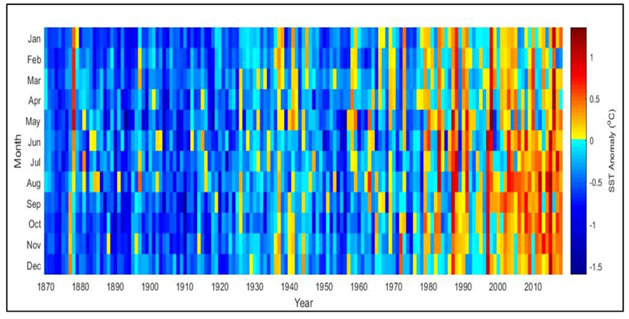
Figure 3 depicts long-term variations in SST anomalies in the GoM from 1870 to 2018. From 1870 to 1970, the SST anomaly was almost 0 or less, ranging between 0 and −1.5 °C, except in 1877. However, from 1970 to 2018, a positive anomaly was detected, ranging between 0.01 and more than 1 °C. The largest positive anomalies were observed between 2005 and 2018. In brief, higher positive changes in SST anomaly were mainly observed mainly between 1998 and 2018.

During the study period, continuous increasing and decreasing trends were observed in the mean yearly SST in the GoM. From 1870 to 1874, there was a decrease in the mean yearly SST from 27.97 ± 0.31 °C to 27.6 ± 0.31 °C. From 1874 to 1878, there was an increase in the mean yearly SST from 27.6 ± 0.31 °C to 28.6 ± 0.31 °C. From 1878 to 1926, a decreasing trend was observed in the mean yearly SST (from 28.6 ± 0.31 °C to 27.9 ± 0.31 °C). However, from 1926 to 1946, an increasing trend was observed. After 1946, the mean yearly SST markedly decreased, and this trend continued until 1958 (27.5 ± 0.31 °C). From 1958 to 2018, a long-term increasing trend in the mean yearly SST was observed (from 27.5 ± 0.31 °C to 28.6 ± 0.31 °C). From 1870 to 2018, the average mean yearly SST was 28.04 ± 0.31 °C, and it remained below this value from 1870 to 1926, except in 1878 and 1898. From 1927 to 1946, the mean yearly SST exceeded the average value, except in 1934, 1938, 1942, and 1946. From 1947 to 1958, the mean yearly SST was again less than the average range, except in 1954. Finally, from 1959 to 2018, SST exceeded the average range, except in 1966, 1970, 1974, 1976, 1994, and 1998 (Figure 4).

Figure 5 shows changes in the annual SST in the study area from 1870 to 2018. The highest positive and negative changes in SST were recorded in 1996 and 2000, respectively. Positive changes in SST were observed in the range of 0 to +0.7 °C. Negative changes in SST were observed in the range of 0 to −0.8 °C. The highest positive and negative SST changes were observed in 1996 (+0.7 °C) and 1999 (−0.8 °C), respectively. The lowest positive and negative SST changes were observed in 1923 (+0.03 °C) and 1959 (−0.02 °C), respectively.

Figure 6 shows the decadal variation of SST in the study area. The highest and lowest average decadal SSTs were observed from 2010 to 2018 (28.5 ± 0.215 °C) and from 1890 to 1899 (27.75 ± 0.252 °C), respectively. During the study period, the change in SST from 2010 to 2018 and from 2000 to 2009 exhibited the greatest increase (+0.35 °C), whereas the change in SST from 1950 to 1959 and from 1940 to 1949 exhibited the greatest decrease (−0.18 °C).

Figure 7 shows the average SST variation of each 1° × 1° node in the study area from 1870 to 2018. Nodes 1, 5, and 6 exhibited the highest and lowest average SST during the study period, with values of 28.15 ± 0.32 °C, 27.96 ± 0.322 °C, and 27.96 ± 0.314 °C, respectively. Each node demonstrated only an increasing trend in SST from 1870 to 2018 (Figure 8).

3.2. Spatial Variations in SST

Figure 9 shows the spatial variation of the average SST in the GoM from 1870 to 2018. In January and February, SSTs ranged from 27 to 27.5 °C and from 27.5 to 28.3 °C, respectively. In March, SSTs ranged from 28.3 to 28.7 °C. April was the warmest month of the year, with SSTs ranging from 29.5 to 30 °C. After April, a reduction in SSTs was observed until December. In May, SSTs ranged from 29 to 29.5 °C, whereas in June, SSTs ranged from 28 to 28.7 °C. From July to September, SSTs decreased, ranging from 27.2 to 28 °C. However, during October and November, SSTs increased, ranging from 28 to 28.5 °C. The spatial distribution of SSTs was low in December, ranging from 27 to 28 °C. In summary, an increasing trend in SSTs was observed from January to April, a decreasing trend was observed from April to September, and an increasing trend was observed in October and November. In brief, the period between March and May was the warmest period of the year.

Figure 10 depicts the tempospatial changes in SSTs in the GoM from 1870 to 2018, from 1920 to 2018, and from 1970 to 2018. The largest change in tempospatial variation was observed between 1870 and 2018, whereas the smallest change was observed between 1970 and 2018. The tempospatial changes in SSTs in the GoM during 1870–2018, 1920–2018, and 1970–2018 ranged from 0.79 to 0.88 °C, from 0.71 to 0.79 °C, and from 0.51 to 0.64 °C, respectively.

3.3. Seasonal Variation

Figure 11 depicts the seasonal changes in SST in the GoM from 1870 to 2018. From December to February, the average SST variation ranged from 0.55 to 0.7 °C. From March to August, the average SST variation ranged from 0.76 to 0.82 °C. From September to November, the average SST variation ranged from 0.85 to 0.95 °C, finally reaching an average of 0.9–0.95 °C. The frequency of SST variation was high from March to May and low from September to November.

4. Discussion

4.1. SST Variation in the Present Study

Figure 2 depicts the average monthly SST variations for the study area from 1870 to 2018. From January to April/May, an increasing trend in SST was observed, followed by a decreasing trend. According to the Tamil Nadu weather department, an unusually warm climate occurred from January to May. April was the warmest month of the year, with an SST of nearly 29.5 °C. From March to May, SST remained above 29 °C because this is the summer season in the GoM. Throughout the year, SST exceeded 27 °C. Edward et al. [16] reported that SST in the GoM has never been below 26 °C and that in the summer season, it remains above 29 °C. August was the coldest month of the year, with an SST of nearly 27 °C. From August to December, the average SST in the GoM was 27 °C. This is because of the moderate to heavy rainfall during October to mid-December as a result of the northeastern monsoons [17]. Being the warmest among the major oceans, the Indian Ocean plays a critical role in regulating the mean climate and variability of the Asian monsoon, as well as the dynamics over the tropics. During summer, the central-east Indian Ocean is characterized by a warm pool with sea surface temperatures (SST) greater than 28.0 °C, making it highly conducive for enhanced convection. Studies on SST trends during the past half-century have pointed out substantial warming over this warm pool, though the reasons behind this monotonic warming have remained ambiguous. The Indian Ocean is warming faster than the global average, which includes the Gulf of Mannar. This is because tropical oceans get more heat. In the case of the Indian Ocean, the waterbody is landlocked to the north, causing heat accumulation in the northern Indian Ocean, which includes the Gulf of Mannar. Another possible reason is the southwest monsoon circulation, which plays a role in directing the heat of the North Indian Ocean southward and has weakened in recent decades. That may have allowed more heat accumulation in the northern Indian Ocean, including the Gulf of Mannar. El Niño appears as an event through which the Pacific Ocean throws out its heat, which partially gets accumulated in the Indian Ocean via a modified Walker circulation, and this might be one more possible reason.

Figure 4 depicts the annual SST variations in the study area from 1870 to 2018. Throughout the study period, sudden fluctuations in SSTs were observed. This may be due to the effect of the dipole mode index (DMI) on the GoM. Figure 12 depicts SST and DMI variability throughout the study period, with a correlation value of 0.512, indicating a moderate correlation [18]. Changes in SST exhibited a similar trend. The DMI index is an indicator of the east-west temperature gradient across the tropical Indian Ocean, linked to the Indian Ocean dipole or zonal mode. Positive or negative changes in DMI indicate positive or negative changes in SSTs [19].

Figure 6 depicts the decadal SST variations in the study area. The highest and lowest average decadal SST values were recorded between 2010 and 2018 and between 1890 and 1899, respectively. Before 1960, the CO₂ concentration was less than 320 ppm (according to Statista). However, it peaked from 2010 to 2018, reaching 418.2 ppm (according to Statista). This may be the reason for the high decadal SST from 2010 to 2018. The average SST between 2010 and 2018 was 28.4 °C, whereas it was less than 28 °C before 1960. Figure 8 depicts the largest positive SST anomalies from 2010 to 2018.

Figure 9 depicts the spatial variations of the average SST in the GoM from 1870 to 2018. In January and February, SSTs ranged from 27 to 27.5 °C and from 27.5 to 28.3 °C, respectively. In March, SSTs ranged from 28.3 to 28.7 °C. April was the warmest month of the year, with SSTs ranging from 29.5 to 30 °C. After April, a reduction in SST was observed until December. In the GoM, the summer season spans from March to May. From September to December, the reduction in SST observed was primarily due to moderate to heavy rainfall [16,17].

4.2. Possible Causes for Increased SST

Generally, the increase in SST from historical times to the present time in the GoM is primarily attributable to the increase in CO₂. The following are some of the reasons for the CO₂ emissions observed in the area:

First, one of the most likely causes of the increase in CO₂ emissions is the rapid growth of the fishing and maritime industries along the southern coast of India. The industrial revolution began in the early 19th century, when machinery powered by new energy sources started to replace manual labor. As a result of the rapid combustion of fuels, the concentrations of greenhouse gases increased, which may have been the sole possible cause for the increase in CO₂ emissions;

Second, with the development of industries, fishing and maritime activities rapidly grew, resulting in an increase in the operation of fuel-powered fishing vessels. Following this trend, the number of fishing vessels increased in the GoM to increase fishing activity and thus meet the high demand. Currently, 45,488 fishing vessels operate along the coast of Tamil Nadu (MPEDA 2021), indicating an increase in CO₂ emissions in the study area.

Third, with the increase in fishing activities, marine communities are being captured and killed at a rate faster than they can regenerate. As a result, stocks are starting to decline, despite increased fishing activities in an effort to find new locations. This increased fishing effort is a major contributor to the increase in CO₂ emissions because more fuel is consumed.

Fourth, as a result of the overfishing of surface species, stocks have begun to decline; thus, bottom trawling has started to be used to fish from the bottom of the ocean. Bottom trawling is the practice of dragging an open fishing net along the ocean floor. When the net is dragged, the entire coral or marine plant community may be destroyed. These communities play a critical role in balancing the CO₂ content of the oceans. Complete destruction of these communities may result in increased CO₂ emissions.

All these abovementioned factors contribute to increased CO₂ emissions in general. Therefore, they are strongly believed to be the reasons for the increase in SST in the GoM from 1870 to 2018. Figure 13 illustrates the increase in greenhouse gas emissions due to industrialization from 1980 to 2020.

4.3. Importance of the Study for the Future

Figure 14 depicts the potential effect of increased SST as well as the sustainable development goals that cannot be met as a result of the increased SST (in parentheses). Historically [20,21] and in future projections, climate change has been linked to substantial biological changes in the structure and function of marine ecosystems [22,23,24]. These include changes in the distribution and abundance of species at local and global scales as well as modifications to ocean productivity [25,26]. Over the next century, these changes are expected to have a substantial effect on the structure and function of marine ecosystems as well as on ecosystem products and services, including the provision of food from fisheries and aquaculture, the production of oxygen, and the storage of anthropogenic carbon [27,28]. Many studies have predicted future changes in marine life in large marine ecosystems [29], coastal seas [30], and global oceans.

Because SST affects oceanographic and biological processes at various temporal and geographical scales, the rates of change in the structure and function of marine ecosystems are expected to vary across ocean basins [31]. According to Cheung et al. [22] and Pinsky et al. [32], marine organisms respond to increasing ocean temperatures by changing their distribution, with expected regional shifts toward colder, deeper, farther offshore, or polar waters as well as global range expansions toward higher latitudes and range retractions at equatorial boundaries [22,31,33]. In addition, in polar marine ecosystems, regional surface temperatures are increasing twice as rapidly as compared with the global average, causing the Arctic marine animal community to become more boreal and resulting in a greater abundance of boreal species than polar affine species [31,34]. By contrast, the overall species abundance in tropical ocean basins and semi-enclosed seas (e.g., the Mediterranean and Baltic Seas) is expected to decrease with future ocean changes [33]. Changes in SST will result in many aspects, both directly and indirectly, that will affect the marine community in the future. Thus, in the present study, we just checked the SST variability, and in our next study, we will assess the effect of changing SSTs on marine communities. In brief, the distribution and richness of species, the availability of food from fisheries and aquaculture, the generation of oxygen, and the storage of anthropogenic carbon are just a few of the ecosystem services and products that are anticipated to be significantly impacted by changes in SSTs [35,36,37,38,39,40].

5. Conclusions

The long-term temporal and spatial trends in SSTs in the GoM from 1870 to 2018 were explored in this study. The mean highest and lowest SSTs during the study period were 29.85 °C in April and 27.15 °C in August, respectively. Monthly time series data from 1870 to 2018 showed a 0.05 °C cooling trend in SSTs from January to December. The mean annual maximum and minimum SST values were 28.93 °C and 27.45 °C, respectively, in 2015 and 1890. The annual time series showed an increase in SSTs of 0.004 °C from 1870 to 2018, 28.56 °C in 2010–2018, and 27.78 °C in 1890–1889 were the mean values for the highest and lowest decadal SSTs, respectively. A decadal time series showed a 0.04 °C warming trend in SSTs from 1870 to 2018. A decadal time series of SSTs revealed a 0.04 °C warming trend from 1870 to 2018. Between 1870 and 2018, the regional distribution of climatic changes in the GoM exhibited a distinct spatial gradient. Throughout the study period, the region between 6–8° N and 77–78° E was the warmest in the GoM. The above results can lead to a few important conclusions, i.e., firstly, there is a significant mean annual SST increase from historic to present time, and secondly, a significant increase in mean decadal SST also exists. Thirdly, the present decade (2010–2018) of the study period was found to be the warmest decade compared to previous decades. All these findings point to the GoM continuously warming from the past to the present. Finally, the southern part of the GoM was observed with warmer SSTs and the highest changes in SSTs throughout the study period.

References

- Belkin, I.M.; Cornillon, P.; Ullman, D. Ocean fronts around Alaska from satellite SST data. In Proceedings of the American Meteorological Society’s 7th Conference on the Polar Meteorology and Oceanography and Joint Symposium on High-Latitude Climate Variations, Hyannis, MA, USA, 12–16 May 2003; Volume 12. [Google Scholar]
- Rayner, N.A.A.; Parker, D.E.; Horton, E.B.; Folland, C.K.; Alexander, L.V.; Rowell, D.P.; Kent, E.C.; Kaplan, A. Global analyses of sea surface temperature, sea ice, and night marine air temperature since the late nineteenth century. J. Geophys. Res. Atmos. 2003, 108. [Google Scholar] [CrossRef] [Green Version]
- McCarthy, G.D.; Haigh, I.D.; Hirschi, J.J.M.; Grist, J.P.; Smeed, D.A. Ocean impact on decadal Atlantic climate variability revealed by sea-level observations. Nature 2015, 521, 508–510. [Google Scholar] [CrossRef] [PubMed] [Green Version]
- Lan, K.-W.; Kawamura, H.; Lee, M.-A.; Lu, H.-J.; Shimada, T.; Hosoda, K.; Sakaida, F. Relationship between albacore (Thunnus alalunga) fishing grounds in the Indian Ocean and the thermal environment revealed by cloud-free microwave sea surface temperature. Fish. Res. 2012, 113, 1–7. [Google Scholar] [CrossRef]
- Maul, G.A. Introduction to Satellite Oceanography; Springer Science and Business Media LLC: Berlin/Heidelberg, Germany, 1985; p. 3. [Google Scholar]
- Zhou, C.; He, P.; Xu, L.; Bach, P.; Wang, X.; Wan, R.; Tang, H.; Zhang, Y. The effects of mesoscale oceanographic structures and ambient conditions on the catch of albacore tuna in the South Pacific longline fishery. Fish. Oceanogr. 2020, 29, 238–251. [Google Scholar] [CrossRef]
- Chen, X.; Tian, S.; Chen, Y.; Liu, B. A modeling approach to identify optimal habitat and suitable fishing grounds for neon flying squid (Ommostrephes bartramii) in the northwest Pacific Ocean. Fish. Bull. 2010, 108, 1–14. [Google Scholar]
- Zainuddin, M.; Saitoh, S. Detection of potential fishing ground for albacore tuna using synoptic measurements of ocean color and thermal remote sensing in the northwestern North Pacific. Geophys. Res. Lett. 2004, 31, 31. [Google Scholar] [CrossRef]
- Zainuddin, M.; Saitoh, K.; Saitoh, S.-I. Albacore (Thunnus alalunga) fishing ground in relation to oceanographic conditions in the western North Pacific Ocean using remotely sensed satellite data. Fish. Oceanogr. 2008, 17, 61–73. [Google Scholar] [CrossRef] [Green Version]
- Lan, K.-W.; Lee, M.-A.; Chou, C.-P.; Vayghan, A.H. Association between the interannual variation in the oceanic environment and catch rates of bigeye tuna (Thunnus obesus) in the Atlantic Ocean. Fish. Oceanogr. 2018, 27, 395–407. [Google Scholar] [CrossRef]
- Kumaraguru, A.K.; Joseph, V.E.; Marimuthu, N.; Wilson, J.J. Scientific information on Gulf of Mannar-A bibliography; Gulf of Mannar Marine Biosphere Reserve Trust: Ramanathapuram, India, 2006. [Google Scholar]
- Edward, J.K.P.; Mathews, G.; Raj, K.D.; Thinesh, T.; Patterson, J.; Tamelander, J.; Wilhelmsson, D.; Yellowlees, D.; Hughes, T.P. Coral reefs of Gulf of Mannar, India: Signs of resilience. Prevalence 2012, 10, 100. [Google Scholar]
- Luis, A.J.; Kawamura, H. Characteristics of atmospheric forcing and SST cooling events in the Gulf of Mannar during winter monsoon. Remote Sens. Environ. 2001, 77, 139–148. [Google Scholar] [CrossRef]
- Achuthankutty, C.T.; Kakodkar, A.; Nath, A.I.V. Indobis and Its Relevance to the Gulf of Mannar Biosphere Reserve. 2008. Available online: https://drs.nio.org/drs/bitstream/handle/2264/1463/Biodiv_Conserv_Gulf_Mannar_Bios_Res_2007_299.pdf?sequence=3&isAllowed=y (accessed on 15 October 2022).
- Krishnan, P.; Purvaja, R.; Sreeraj, C.R.; Raghuraman, R.; Robin, R.S.; Abhilash, K.R.; Mahendra, R.S.; Anand, A.; Gopi, M.; Mohanty, P.C.; et al. Differential bleaching patterns in corals of Palk Bay and the Gulf of Mannar. Curr. Sci. 2018, 2018, 679–685. [Google Scholar] [CrossRef]
- Edward, J.K.P.; Mathews, G.; Raj, K.D.; Tamelander, J. Coral reefs of the Gulf of Mannar, Southeastern India-observations on the effect of elevated SST during. In Proceedings of the 11th International Coral Reef Symposium, Ft. Lauderdale, FL, USA, 7–11 July 2008. [Google Scholar]
- Asir, N.; Kumar, P.D.; Arasamuthu, A.; Mathews, G.; Raj, K.D.; Kumar, T.K.; Bilgi, D.S.; Edward, J.K. Eroding islands of Gulf of Mannar, Southeast India: A consequence of long-term impact of coral mining and climate change. Nat. Hazards 2020, 103, 103–119. [Google Scholar] [CrossRef]
- Saji, N.H.; Goswami, B.N.; Vinayachandran, P.N.; Yamagata, T. A dipole mode in the tropical Indian Ocean. Nature 1999, 401, 360–363. [Google Scholar] [CrossRef]
- Ratner, B. The correlation coefficient: Its values range between+ 1/− 1, or do they? J. Target. Meas. Anal. Mark. 2009, 17, 139–142. [Google Scholar] [CrossRef] [Green Version]
- Harnik, P.G.; Lotze, H.K.; Anderson, S.C.; Finkel, Z.V.; Finnegan, S.; Lindberg, D.R.; Liow, L.H.; Lockwood, R.; McClain, C.R.; McGuire, J.L.; et al. Extinctions in ancient and modern seas. Trends Ecol. Evol. 2012, 27, 608–617. [Google Scholar] [CrossRef]
- Yasuhara, M.; Danovaro, R. Temperature impacts on deep-sea biodiversity. Biol. Rev. 2016, 91, 275–287. [Google Scholar] [CrossRef] [Green Version]
- Cheung, W.W.; Lam, V.W.; Sarmiento, J.L.; Kearney, K.; Watson, R.; Pauly, D. Projecting global marine biodiversity impacts under climate change scenarios. Fish Fish. 2009, 10, 235–251. [Google Scholar] [CrossRef]
- Pecl, G.T.; Araújo, M.B.; Bell, J.D.; Blanchard, J.; Bonebrake, T.C.; Chen, I.C.; Clark, T.D.; Colwell, R.K.; Danielsen, F.; Evengård, B.; et al. Biodiversity redistribution under climate change: Impacts on ecosystems and human well-being. Science 2017, 355, eaai9214. [Google Scholar] [CrossRef]
- Worm, B.; Lotze, H.K. Marine biodiversity and climate change. In Climate and Global Change: Observed Impacts on Planet Earth; Letcher, T., Ed.; Elsevier: Amsterdam, The Netherlands, 2016; pp. 195–212, Chapter 13. [Google Scholar]
- Boyce, D.G.; Lewis, M.R.; Worm, B. Global phytoplankton decline over the past century. Nature 2010, 466, 591–596. [Google Scholar] [CrossRef]
- Moore, J.K.; Fu, W.; Primeau, F.; Britten, G.L.; Lindsay, K.; Long, M.; Doney, S.C.; Mahowald, N.; Hoffman, F.; Randerson, J.T. Sustained climate-warming drives declining marine biological productivity. Science 2018, 359, 1139–1143. [Google Scholar] [CrossRef] [Green Version]
- Pörtner, H.O.; Knust, R. Climate change affects marine fishes through the oxygen limitation of thermal tolerance. Science 2007, 315, 95–97. [Google Scholar] [CrossRef] [PubMed] [Green Version]
- Vichi, M.; Manzini, E.; Fogli, P.G.; Alessandri, A.; Patara, L.; Scoccimarro, E.; Masina, S.; Navarra, A. Global and regional ocean carbon uptake and climate change: Sensitivity to a substantial mitigation scenario. Clim. Dyn. 2011, 37, 1929–1947. [Google Scholar] [CrossRef]
- Blanchard, J.L.; Jennings, S.; Holmes, R.; Harle, J.; Merino, G.; Allen, J.I.; Holt, J.; Dulvy, N.K.; Barange, M. Potential consequences of climate change for primary production and fish production in large marine ecosystems. Philos. Trans. R. Soc. B Biol. Sci. 2012, 367, 2979–2989. [Google Scholar] [CrossRef] [PubMed]
- Barange, M.; Merino, G.; Blanchard, J.L.; Scholtens, J.; Harle, J.; Allison, E.H.; Allen, J.I.; Holt, J.; Jennings, S. Impacts of climate change on marine ecosystem production in societies dependent on fisheries. Nat. Clim. Change 2014, 4, 211–216. [Google Scholar] [CrossRef]
- Fossheim, M.; Primicerio, R.; Johannesen, E.; Ingvaldsen, R.B.; Aschan, M.M.; Dolgov, A.V. Recent warming leads to a rapid borealization of fish communities in the Arctic. Nat. Clim. Change 2015, 5, 673–677. [Google Scholar] [CrossRef]
- Pinsky, M.L.; Worm, B.; Fogarty, M.J.; Sarmiento, J.L.; Levin, S.A. Marine taxa track local climate velocities. Science 2013, 341, 1239–1242. [Google Scholar] [CrossRef] [Green Version]
- Cheung, W.W.; Watson, R.; Pauly, D. Signature of ocean warming in global fisheries catch. Nature 2013, 497, 365–368. [Google Scholar] [CrossRef]
- Hoegh-Guldberg, O.; Bruno, J.F. The impact of climate change on the world’s marine ecosystems. Science 2010, 328, 1523–1528. [Google Scholar] [CrossRef]
- Tonelli, M.; Signori, C.N.; Bendia, A.; Neiva, J.; Ferrero, B.; Pellizari, V.; Wainer, I. Climate projections for the southern ocean reveal impacts in the marine microbial communities following increases in sea surface temperature. Front. Mar. Sci. 2021, 8, 636226. [Google Scholar] [CrossRef]
- Alexander, M.A.; Scott, J.D.; Friedland, K.D.; Mills, K.E.; Nye, J.A.; Pershing, A.J.; Thomas, A.C. Projected sea surface temperatures over the 21st century: Changes in the mean, variability and extremes for large marine ecosystem regions of Northern Oceans. Elem. Sci. Anthr. 2018, 6, 9. [Google Scholar] [CrossRef] [Green Version]
- Sweijd, N.A.; Smit, A.J. Trends in sea surface temperature and chlorophyll-a in the seven African Large Marine Ecosystems. Environ. Dev. 2020, 36, 100585. [Google Scholar] [CrossRef]
- Gittings, J.A.; Raitsos, D.E.; Krokos, G.; Hoteit, I. Impacts of warming on phytoplankton abundance and phenology in a typical tropical marine ecosystem. Sci. Rep. 2018, 8, 1–12. [Google Scholar] [CrossRef]
- Popova, E.; Yool, A.; Byfield, V.; Cochrane, K.; Coward, A.C.; Salim, S.S.; Gasalla, M.A.; Henson, S.A.; Hobday, A.J.; Pecl, G.T.; et al. From global to regional and back again: Common climate stressors of marine ecosystems relevant for adaptation across five ocean warming hotspots. Glob. Change Biol. 2016, 22, 2038–2053. [Google Scholar] [CrossRef] [Green Version]
- Tommasi, D.; Stock, C.A.; Alexander, M.A.; Yang, X.; Rosati, A.; Vecchi, G.A. Multi-annual climate predictions for fisheries: An assessment of skill of sea surface temperature forecasts for large marine ecosystems. Front. Mar. Sci. 2017, 4, 201. [Google Scholar] [CrossRef]
Figure 1.
Bathymetry of the study area.
Figure 2.
Average monthly SST variation in the study area from 1870 to 2018. Black straight lines indicate the standard error.
Figure 3.
Long-term variations of SST anomalies in all years and months in the Gulf of Mannar (GoM) from 1870 to 2018.
Figure 4.
Annual SST variation in the study area from 1870 to 2018. The red line indicates the average SST (28.04 °C) during the study period. The black, straight lines indicate the standard deviation limits.
Figure 5.
Changes in the mean annual SST in the study area from 1870 to 2018. The black, straight lines indicate the standard error.
Figure 6.
Decadal SST variation in the study area from 1870 to 2018. The black, straight lines indicate the standard error.
Figure 7.
Average SST variation of each 1° × 1° node in the study area. The black, straight lines indicate the standard error.
Figure 8.
Annual SST variation of each 1° × 1° node (nine nodes) in the study area from 1870 to 2018.
Figure 9.
Spatial variation of average SSTs in the GoM from 1870 to 2018.
Figure 10.
Spatial changes in SSTs in the GoM from (a) 1870–2018, (b) 1920–2018, and (c) 1970–2018.
Figure 11.
Seasonal changes in SST in the GoM from 1870 to 2018.
Figure 12.
(a) SST and dipole mode index (DMI) variability and (b) correlation between SST and DMI throughout the study period.
Figure 13.
Increasing trend of greenhouse gas emissions from 1980 to 2020. Source: https://ccsknowledge.com/what-is-ccs/climate-change (Access date 1 December 2022).
Figure 14.
Potential effects of increased SST in the GoM.
Disclaimer/Publisher’s Note: The statements, opinions and data contained in all publications are solely those of the individual author(s) and contributor(s) and not of MDPI and/or the editor(s). MDPI and/or the editor(s) disclaim responsibility for any injury to people or property resulting from any ideas, methods, instructions or products referred to in the content. |
© 2023 by the authors. Licensee MDPI, Basel, Switzerland. This article is an open access article distributed under the terms and conditions of the Creative Commons Attribution (CC BY) license (https://creativecommons.org/licenses/by/4.0/).
Share and Cite
MDPI and ACS Style
Mondal, S.; Lee, M.-A. Long-Term Observations of Sea Surface Temperature Variability in the Gulf of Mannar. J. Mar. Sci. Eng. 2023, 11, 102. https://doi.org/10.3390/jmse11010102
AMA Style
Mondal S, Lee M-A. Long-Term Observations of Sea Surface Temperature Variability in the Gulf of Mannar. Journal of Marine Science and Engineering. 2023; 11(1):102. https://doi.org/10.3390/jmse11010102
Chicago/Turabian StyleMondal, Sandipan, and Ming-An Lee. 2023. "Long-Term Observations of Sea Surface Temperature Variability in the Gulf of Mannar" Journal of Marine Science and Engineering 11, no. 1: 102. https://doi.org/10.3390/jmse11010102
Note that from the first issue of 2016, this journal uses article numbers instead of page numbers. See further details here.