Marine GIS as a Tool to Support Backscatter Data Analysis for Zooplankton Investigations

Abstract

Echo-sounders and Vessel-Mounted Acoustic Doppler Current Profilers (VM-ADCP) are widely operating onboard research vessels with the aim of providing real-time backscatter and ocean current profiles along the route, while the vessel is moving. Backscatter data are exploited to infer important information about zooplankton presence and distribution. Nevertheless, as these organisms daily vertically migrate even below the depth of the instrument range, the combination of space and time variability make their mapping from a moving vessel quite complex. The objective of this work is to describe a GIS application developed for the management and analysis of these data. The GIS capability as a tool to facilitate zooplankton investigations is assessed by means of a test-case in the area of the Ligurian Sea (Western Mediterranean) by using VM-ADCP backscatter data made available during oceanographic campaigns. The system, which includes a high-resolution bathymetry, environmental parameters, ephemeris, allows to select and visualize data sorted according to all the possible layer combinations. Moreover, different backscatter profiles, characterizing the identified migration phases can be enlightened by means of false color scale representation.

1. Introduction

Remotely active acoustic measurements at frequencies in the range of a few hundred kHz are widely exploited to investigate zooplankton abundance and distribution in the oceans and lakes [1,2,3].

Acoustic Doppler Current Profilers (ADCPs) are powerful instruments for the measurements of 3D ocean currents profiles up to great depths, exploiting the Doppler shift of an acoustic signal backscattered by the particles transported by the currents [4]. As ADCPs operate at frequencies in the range of a few hundred kHz, it was soon discovered that the estimation of the vertical velocity was affected—even not almost completely determined—by the presence of migrating zooplankton [5,6]. Despite ADCPs not being designed with the aim of acoustic detection, starting from the 1990s many scientists have successfully analyzed the ancillary backscatter data obtained by the ADCP to extract information about the distribution and abundance of zooplankton [7,8,9,10].

VM-ADCPs are usually mounted in the ships’ hull or a retractable keel, to perform continuous current profiles along the route and are now regularly operating onboard most of the research vessels. Even if they are primarily used for current measurements, the huge amount of continuous acoustic backscatter data is made available during oceanographic campaigns, and these data represent a precious source of additional information that can support further environmental and biological investigations. Nevertheless, in many cases, in particular when the experiments focus on different objectives, they are not properly archived, with the risk that they become lost.

This paper describes a GIS application developed for the management, elaboration and visualization of acoustic backscatter data to facilitate the analysis of zooplankton distribution and variability.

Zooplankton spatial distribution can be characterized by a noteworthy daily and sub-daily vertical migration up to some hundred meters and covers a wide range of temporal variability related to meteorological, oceanographic and climatic conditions [11,12,13,14,15,16,17].

Acoustic devices operating from fixed points provide long time series of backscatter data on the water column; this allows the analysis of phenological indices related to organism’s migration such as the timing of initiation and termination, peak and duration [18,19], but does not provide information on their spatial distribution.

Despite the improvements in understanding and modeling the response of zooplankton organism to the acoustic frequencies, remote acoustic detection still fails to provide reliable information about the species composition [20]. Such information can be only obtained from the analysis of in situ samples collected during at sea experiments with nets or by continuous plankton recording that are highly time-consuming and seldom satisfy the spatial-temporal resolution required for a 3D synoptic view over a wide basin, as the spatial pattern is strongly modified by the daily vertical migrations.

In this context, geographic information systems (GIS), due to their capability to integrate and visualize spatial data, have proven to be an efficient tool for the management of heterogeneous data and can be of advantage for scientific investigations specifically devoted to marine environmental studies. Most of the applications rely on the possibility to merge model data, satellite observations and in situ measurements, facilitating data interpretation and enlightening existing relations among different environmental parameters [21,22,23,24].

The described Q-GIS tool developed by the Italian Hydrographic Service has the aim to preserve and provide added value to the acoustic backscatter data collected during oceanographic and hydrographic campaigns as a support to studies on zooplankton migration.

The area chosen for the test case is the Ligurian Sea, which hosts a rich ecosystem compared to the rest of the Mediterranean Sea and includes two Marine Protected Areas and the Whale Sanctuary, whose population depends on zooplankton biomass. Anchovies are among the more required species in the basin and their abundance strictly depends on annual zooplankton availability, making its knowledge of great importance for a sustainable fishing management. This precious natural environment coexists with a high coastal urbanization and industrialization and experiences some of the most maritime traffic in the Mediterranean, and hence needs sound environmental assessments as a first step to control its trophic state and ecological potential.

For the evaluation of the implemented Q-GIS tool, we took into consideration the main factors influencing the zooplankton migratory pattern along the water column, and in particular, the daily cycle and the meteorological and oceanographic conditions. The test also included multispectral analysis and false color composition technique for the analysis and representation of the vertical structure. VM-ADCP data used for the test-case were acquired during oceanographic campaigns in the Ligurian Sea and concurrent time series from fixed moorings in the same region, as well as meteorological and oceanographic data, which were used to support the findings of this study.

The paper is structured as follows: Section 2 provides an overview of the used data set and the implemented software tool; Section 3 is devoted to the description of the observed migration pattern; Section 4 shows the capability of the proposed tool to effectively support scientists in the data analysis; results are discussed in Section 5.

2. Tools and Methodologies

2.1. Data Set for the Test Case

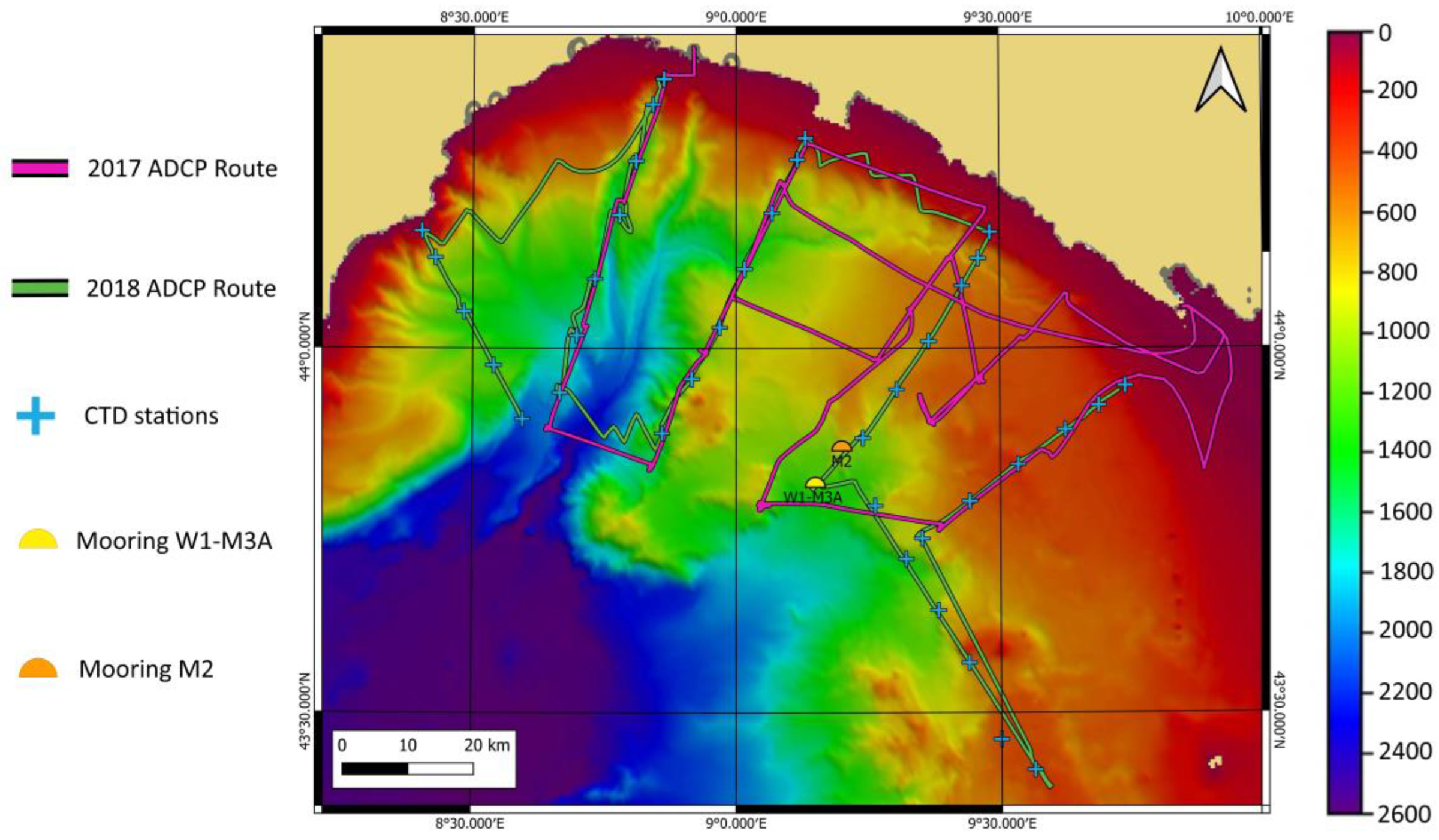
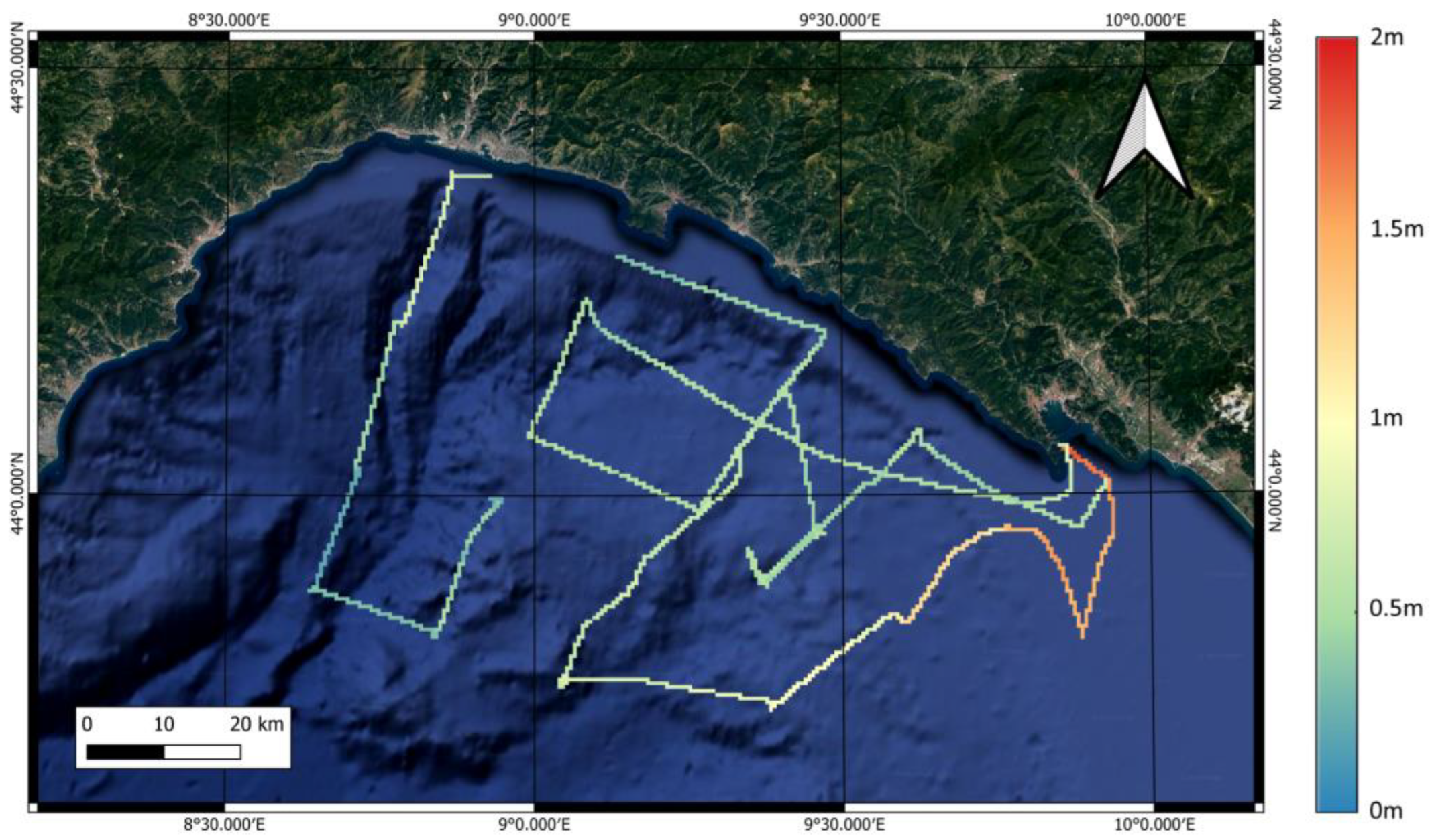
During 2017–2018, several oceanographic experiments took place in the Central and Eastern part of the Ligurian Sea and even if planned to fulfil different scientific purposes, all the experiments included ADCP measurements, from both fixed moorings and moving vessels. Two oceanographic campaigns were carried out along similar routes, the first during April 2017 onboard N/O MINERVA, operated by the National Research Council of Italy (CNR), and the second on September 2018 onboard R/V ARETUSA, operated by the Italian Hydrographic Institute (IIM).

Time-series of ADCP data from the fixed position were obtained during the period 30 March–29 August 2017 from a Nortek Aquadopp Profiler (400 kHz) operated by ENEA and located on the W1-M3A observatory, in the center of the Ligurian Sea [25] on a sea bed of 1200 m operating in the first 30 m of the water column in an upward looking configuration.

The other time series of ADCP data was collected from a fixed mooring (referred to as M2) deployed at 43.865° N; 09.200° E by NATO-CMRE in the framework of the LOGMEC17 experiment [26]. The sea depth was 1020 m and the ADCP sampled the water column from the depth of 250 m up to the near-surface for about two months (14 September–14 November 2017).

The time and position associated with each profile has been acquired with DGPS FUGRO 9205 GNSS with Marinestar HP+G2 corrections.

Details of the ADCP measurement and their spatial and temporal coverage are described in the

Table 1. Details of the analyzed acoustic dataset provided by deployed ADCPs.

Period	Cruise/Observatory	Region/Position	ADCP Model	Layer [m]	Depth of the Cell [m]	Sampling Period [min]
20–25 April 2017	CNR-MINERVA	Central-Eastern Ligurian Sea	RDI VM-150 kHz	0–250	4	5
3–6 September 2018	IIM-ARETUSA	Central-Eastern Ligurian Sea	RDI VM-150 kHz	0–250	4	10
30 March–29 August 2017	W1-M3A	43.815° N, 09.1133° E	Nortek Aquadopp Profiler 400 kHz	0–32	4	30
13 September–14 November 2017	Mooring M2	43.864° N 09.2000° E	RDI Quartermaster 150 kHz	0–250	8	15

, whereas the route of the campaigns along with the CTD sampling position are displayed in Figure 1.

The acoustic data-set obtained during the two campaigns was chosen for the test case to prove the capabilities of the developed GIS, while data from fixed mooring allowed one to better characterize zooplankton migrations in the area and was useful as a reference test for modal decomposition. Sea temperature and salinity profiles obtained during the campaigns are also included, whereas information about the presence and composition of zooplankton were obtained from some net samples collected during the campaign of April 2017.

Bathymetry and topography used for the GIS is based on the high-resolution bathymetry rasters acquired, and processed by the IIM and Ephemeris are those computed each year by IIM.

2.2. Q-GIS

Data acquired by the ADCPs have both temporal and spatial (horizontal and vertical) variability, and the use of a GIS allows one to consider several variables into the same system and integrate them with each other. For the purposes of this work, among the various GIS systems, it was chosen QGIS^®, a widely used open-source professional GIS application developing a plugin in the Python programming language.

ADCP and CTD data were integrated along with their GNSS time and position (ETRF2014), in order to create a raw dataset to be processed.

To represent a comprehensible integration between the analyzed parameters, false color techniques are also available: these techniques, mainly devised for the analysis of multispectral radiometric images (satellite or aerial photos), consist of color rendering methods to obtain false color images. Each band of the image (usually wavelength regions of electromagnetic radiation) is associated with a different color of the visible light of human eyes (red, green and blue) and the resulting false color image highlights details that otherwise are not easily recognizable. The process used in this work consists in creating multilayer images with acoustic layers (and qualitative parameters) instead of electromagnetic bands.

2.3. Relative versus Absolute Values: Mean Volume Backscatter Computation

Raw acoustic data underwent a post-processing to make them comparable, as they are generated by different instruments. To this end, the Mean Volume Backscatter Strength (Sv) in dB rel (4πm)⁻¹ was computed according to [27] with the improvements suggested by [28] and [29] and reported in Equation (A1). Hereafter, for the sake of brevity, the unit will simply be referred to as dB.

The information about instrument characteristics is provided by the manufacturers; the sound absorption coefficients were computed following [30], the environmental parameters were selected from the CTD cast in the points closest both in time and space (using their GNSS data) to the ADCP profile. Moreover, to consider the effects of the attenuation with the depth, the slant range (R) was included in the computation and a 4-D matrix (Lat, Lon, Depth, time) of Sv in dB was obtained.

The script was developed using Python, which is compatible with Q-GIS and was integrated as a plug-in and data elaboration tool. For this test-case, the tool was specifically designed for RDI ADCP data processing, but software for ADCPs of other manufacturers can be developed and integrated. The complete formulas are reported in Appendix A.

3. Migration Patterns’ Characterization

Zooplankton has an essential role in the marine food chain, being the link between the higher trophic levels and phytoplankton, which are primary producers in the marine environment and represent preys of big cetaceans and fish, which, in turn, sustain top predators. Modulation of such particular behaviors of these organisms is of great interest for marine environmental science as well as for fish management. Several investigations of zooplankton carried out in the Ligurian Sea allowed one to characterize species composition, distribution and migration patterns in this region [31,32,33]. Most of the results from past experiments were obtained by net sampling; only starting from the 2000s, long-term time series from acoustic devices and ADCP backscatter data were also exploited [34,35].

In general, nocturnal migration is the most common pattern and involves the upward movement of zooplankton at dusk to feed on phytoplankton, and they descend at dawn, staying at a depth during the day where the probability of being predated by a visually hunting predator is higher. Other two patterns are recognized: reverse migration when organisms tend to stay at surface during the day and move downward at night and, less common, twilight migration, distinguished by ascent at dusk and sunrise, descent at midnight and immediately after sunrise [36]. These latter migration patterns have the advantage of avoiding other nocturnal migrators, such as non-visually hunting invertebrate predators or simply competitors.

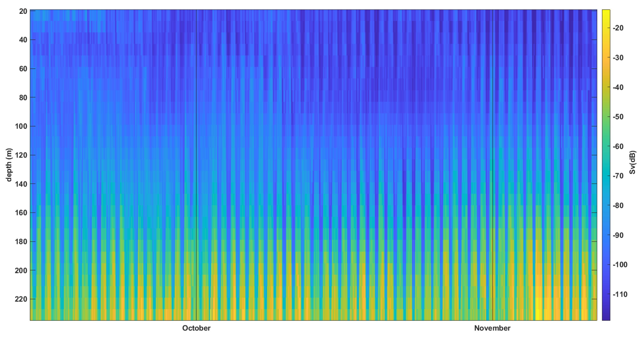
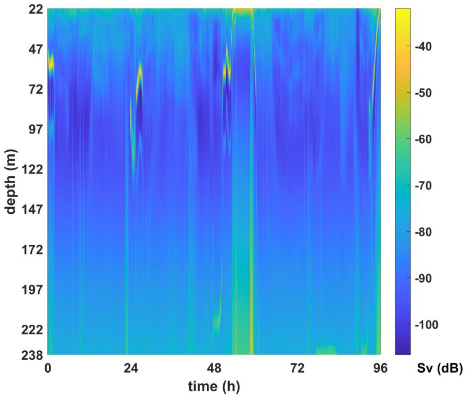
Additional ADCP time series, as reported in Table 1, and partly concurrent with the data from the oceanographic campaigns, are here analyzed to characterize the zooplankton migration during the test case, covering the period from spring to late autumn. As the cyclic variation in the backscatter intensity is mostly related to the migration, a time-frequency analysis of acoustic data proved to be a good method to identify the presence of zooplankton over long periods and, as an example, the variation of the duty cycle of day/night from early September to late November is well identified in the backscatter time series of mooring M2 (Figure 2). The limit of acoustic detection is that it requires accurate in situ calibration with biological samples to quantify the biomass, otherwise only qualitative information can be extracted.

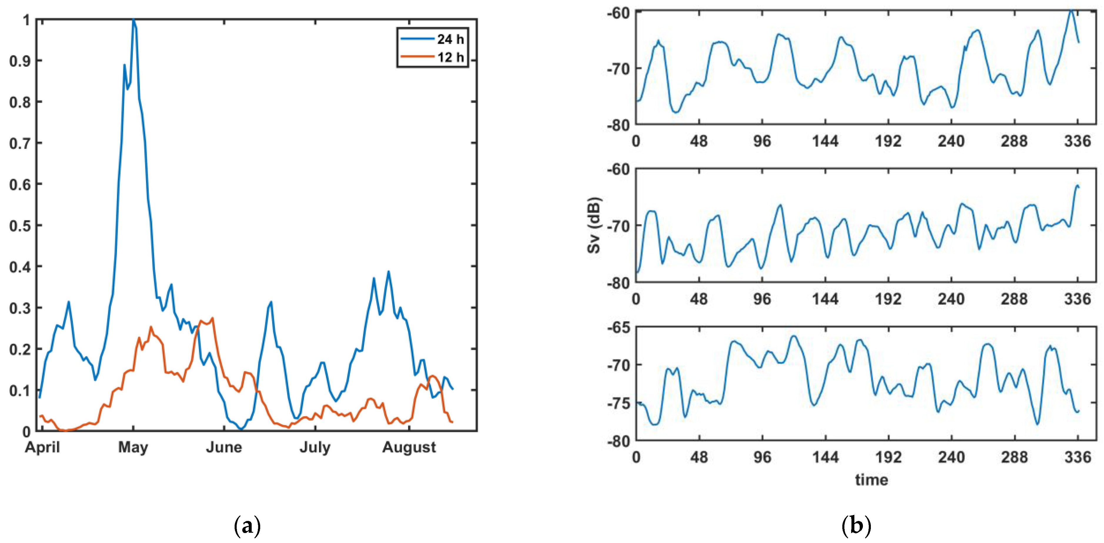
This good correspondence between acoustic backscatter and periodic zooplankton migration allows the application of time-frequency methods, which are here used to objectively detect the occurrence and the relative contribution of 24 and 12-h migration periods at the different depths.

Fast Fourier Transform (FFT) spectra were performed using a 10-days window for the first time series (W1-M3A) and 6 days for the second (M2), due to its limited length with a time step of 24 h for both. The signals’ amplitude of the harmonic associated with 24-h and 12-h period was extracted and the resulting time-series analyzed (Figure 3): high values indicate the prevalence of migration with the selected periodicity and can help to provide information about the behaviors of the community.

Daily migration was found dominant during the whole analyzed period, with peaks lasting about two weeks, the most relevant occurring in mid-May and October in agreement with the known delay of one month in zooplankton bloom, with respect to the peak of surface primary production.

Semidiurnal and mixed migration patterns were also identified, but their contribution to the backscatter signal was of less importance, indicating a smaller amount of backscatter from species having this behavior: highest values were found from mid-May to early June and no significant correlation was found between the two series. Nevertheless, as the backscatter is related to the dimension of the scatterers, the possibility must be considered of large uncertainties ascribed to the use of only one frequency in the acoustic detection, which can miss smaller organisms.

Preliminary investigations on time series W1-M3A [37] did not reveal significant relations between migration and lunar cycle, mainly for the absence of clear nights during full moon lunar-phases in the analyzed period.

4. Test-Case for GIS Applications

The test-case described in this chapter aims at demonstrating the advantage of the use of the developed Q-GIS tool to support zooplankton investigations, and specifically, the analysis of zooplankton spatial distribution and its relation with the migration phase, and meteorological and oceanographic conditions, are addressed in the reported examples.

4.1. Setting the Geographical Domain

The geographical boundaries were set by using high-resolution bathymetry rasters acquired and processed by IIM on an area of a more than 3000 m deep basin, opened to the Southwest and characterized by a narrow shelf [38]. Important and deep canyons are stemming from the coasts in front of Genoa and eastward close to Bonassola, which, due to the strong bottom currents and the considerable contribution of suspended sediments and organic substances, creates environments favorable to the development and growth of valuable ecosystems such as deep corals [39,40] and are perfect areas for backscatter data analysis.

The shelf narrows to the west, while in the eastern part, in the Gulf of La Spezia, it flattens, reaching a depth of only a few tenths of meters. The connection with the Tyrrhenian Sea in the east occurs through the Corsica Channel, a 400 m, sill which prevents the deep waters’ exchange between the two basins.

Sea depth dataset are also used for quality check procedures, since it is known that the ADCP, when operating at depths lower than the instrument range, is strongly affected by the presence of the bottom; the data cannot be considered valid, and the cross-checking with the bathymetry allows one to discard the anomalous high backscatter values due to the presence of the bottom.

To better characterize the geographical and environmental domain, in addition to the salinity and temperature profiles obtained during the campaigns, the system can manage layers with horizontal maps of data from different sources such as in situ and satellite observations, as well as models’ results and climatology data-set.

4.2. Day and Night; Lunar Phases

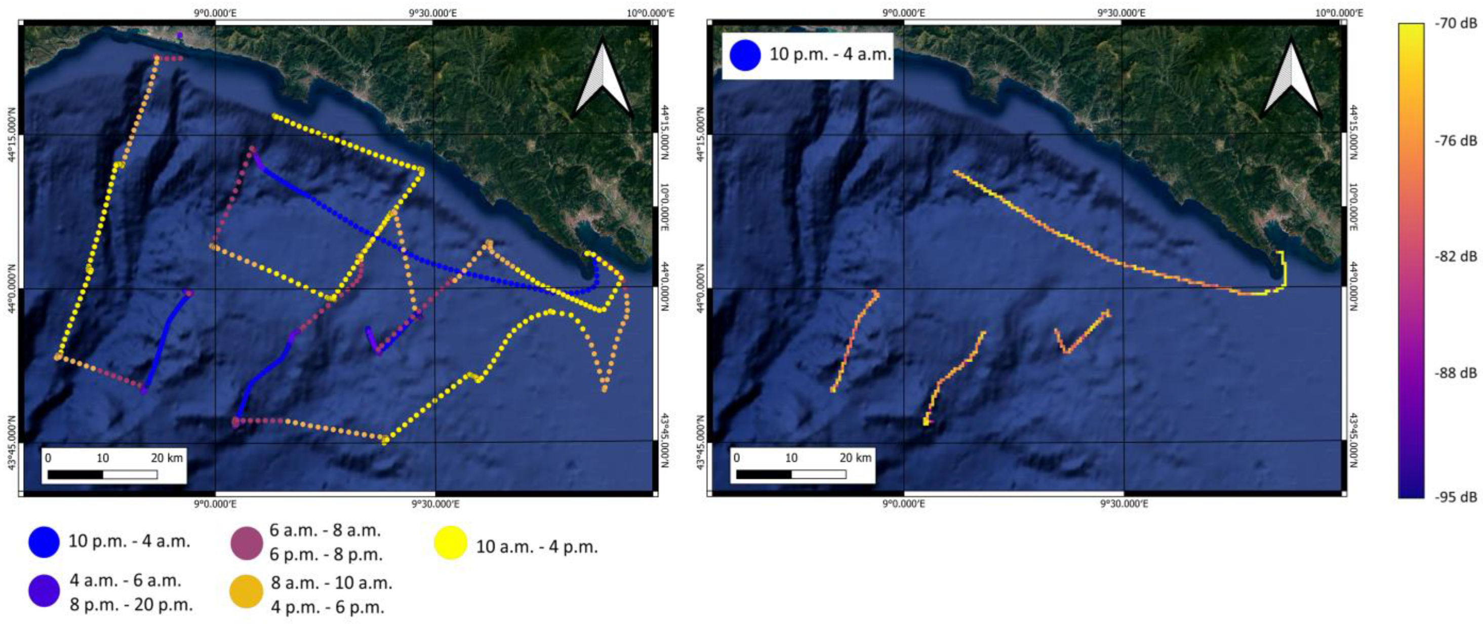
Most of the zooplankton organisms vertically migrate from deep layers, where they are generally found during the day, to the surface, which is reached after dusk.

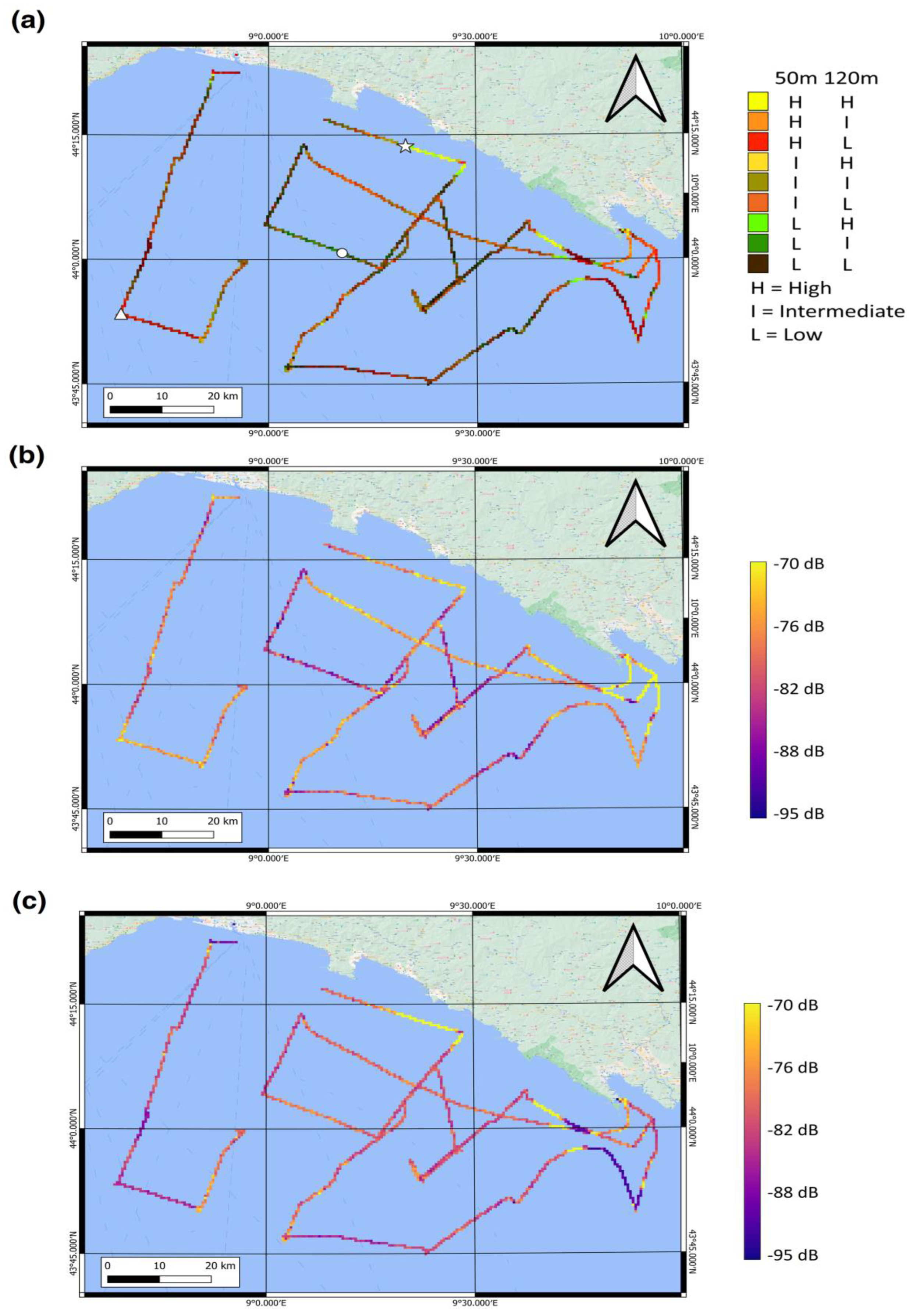
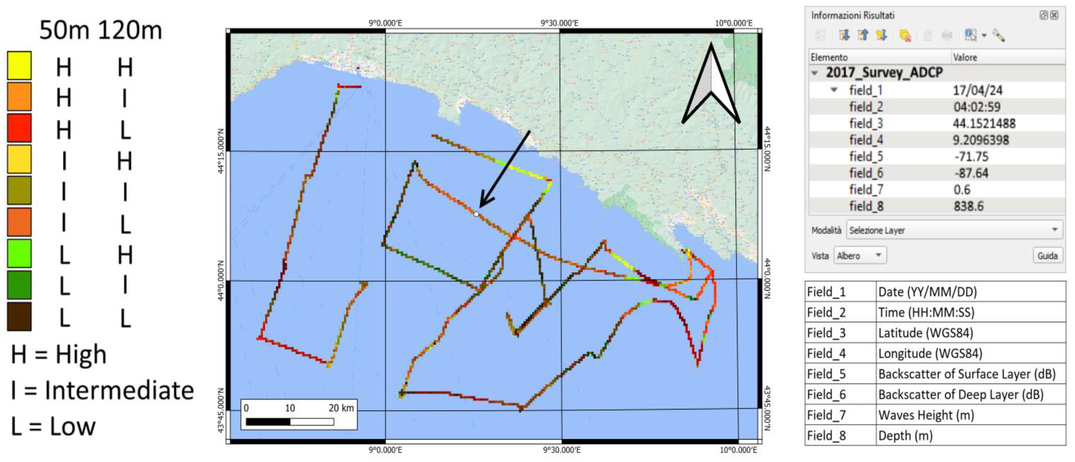
The use of the ephemeris allows one to precisely identify and select the profiles collected at a time corresponding to the different phases of the day-light (dusk, night, dawn and day), which are represented in the maps by different colors (in the left panel of Figure 4 night is blue, day is yellow, and dusk and dawn are purple). The same analogy can be applied to select the data according to the lunar phases, which are known to influence the migrating behavior. GNSS time is integrated in the acoustic georeferenced data: GIS allows one to automatically extract the profiles included within defined time ranges.

This can help for a better interpretation of the spatial distribution, as all the data are taken during the same migration phase; this is particularly useful when working over a large region, where the time required for the monitoring activities is not consistent with a synoptic view.

In the reported example, backscatter strength values at 50 m collected during the night period (blue dot in Figure 4 on the left side) are selected and represented in the right panel of Figure 4. It shows relatively high backscatter values and a quite uniform spatial variability.

4.3. Vertical Structure and Horizontal Distribution: False Color Composition

GIS have been mainly devised with the aim of managing and representing horizontal spatial data, and the application to the marine environment also requires one to represent and analyze the vertical distribution of relevant environmental parameters along the water column.

Generally, this is accomplished by mapping the horizontal distribution at different depths: when the profiles can be described with an appropriate metric, which associates a single to value each profile, the GIS has the advantage of allowing a horizontal overview of the vertical structure below. An example is the mixed layer depth, which is an important value that, along with surface temperature, well describe the sea temperature profile.

Vertical profiles of acoustic backscatter strongly change their shape with time and space due to the zooplankton daily migration as well as a response to local environmental conditions or according to the seasonal cycle. The feasibility of false color composition technique to help to identify the main vertical structure of acoustic profiles from a surface map is here assessed.

4.3.1. Empirical Orthogonal Function Analysis

Modal decomposition techniques are widely used in atmospheric and earth science to reconstruct profiles or 2D fields (generally surfaces) as a linear combination of a number of defined profiles (or surfaces), the so-called modes [41]. This allows one to infer the vertical structure of the data and the dominant shape from the values of each coefficient; although modal decomposition is the result of mathematical computation (such as eigenvectors and eigenvalues), for most of the application, each mode can be associated to a statistical or to a physical property of the analyzed parameter, thus facilitating the data interpretation and the relation with specific forcing.

To display and localize the relative contribution of each mode in a GIS, the function of false color composition is of great advantage when the signal can be described by a linear combination of two or three coefficients, since if we associate a basic color to each coefficient, the resulting color will be the linear combination of them. To simplify, if we associate the blue to the first mode coefficient and the red to the second mode, a magenta dot on the map will represent a situation of equal contribution percentage from the two modes.

The capacity of modal decomposition to represent the acoustic backscatter profiles was firstly tested on the time series collected by the ADCP, located in mooring M2, where Empirical Orthogonal Function (EOF) analysis was applied [42]. Before the analysis, the time series was firstly smoothed with a 5-step moving average and then hourly mean data were computed; the number of vertical levels, which determine the total number of modes, was halved by vertically averaging over two bins.

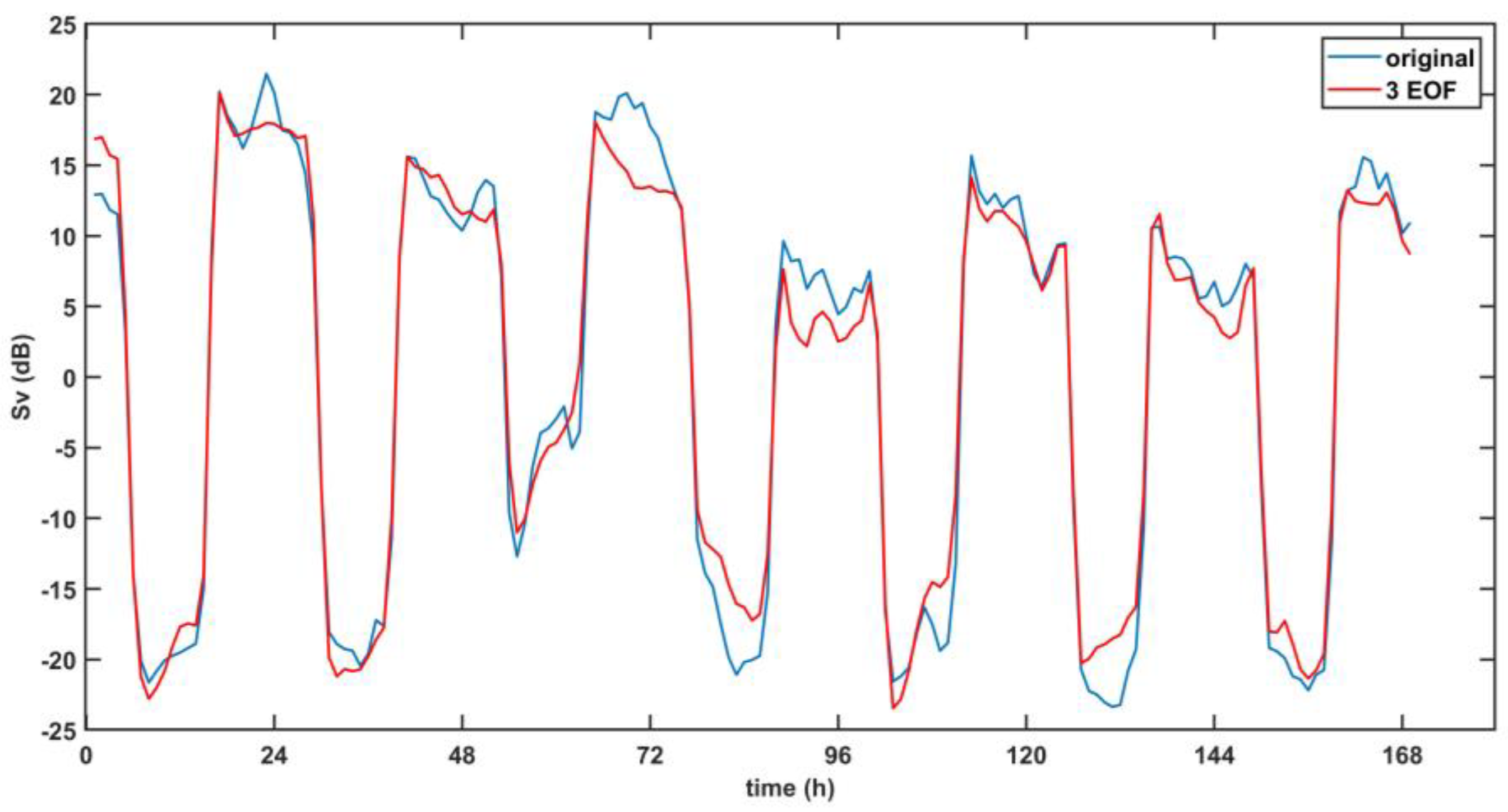
The first three modes are able to account for about 80% of the entire signal, but only even the first two provided good results. The three EOF modes (Figure 5) reproduce the original signal shape and amplitude quite well (Figure 6) but present an almost constant bias of about 20 dB, and miss some surface variability.

Root-mean square error between the signal and the modal reconstruction is 20.8 using three modes and 43.4 with only two, and the time series of the first coefficient display a clear 24-h periodicity well related to the daily migration, as well as a longer-term modulation.

4.3.2. Test Case: False Color Composition

In the reported case-study, a different metric, which ensures an easier and immediate interpretation, is proposed with the advantage that it can be applied even to ADCP profiles collected over a different water column depth, which happens when the vessel passes along coastal regions where the sea depths are lower than the instrument range.

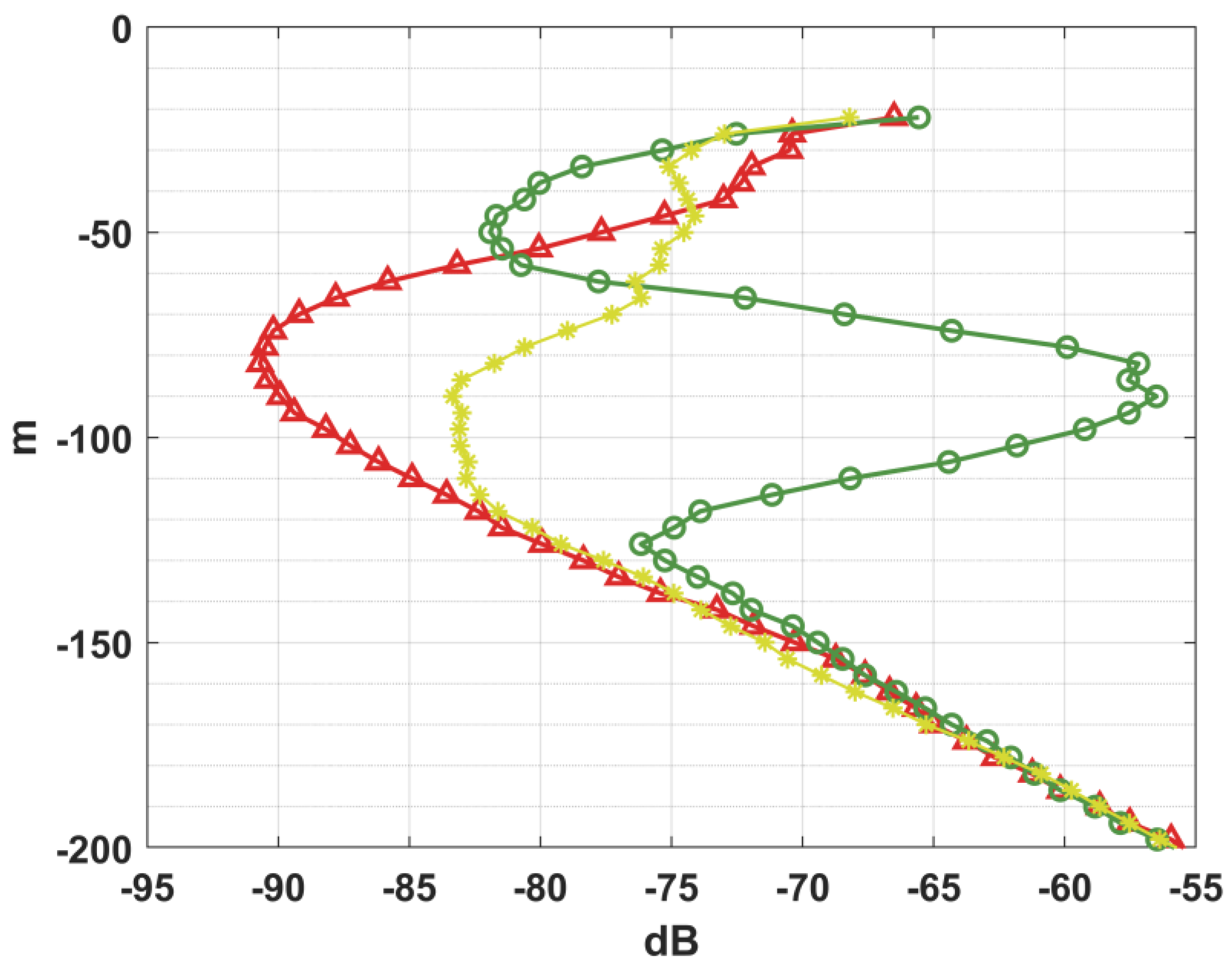
Each profile was characterized in terms of three backscatter value limits at two selected depths describing the situations that better characterize the diel vertical migration: high zooplankton presence at the surface during the night and high zooplankton presence at depths during the day, which allows for all their possible combinations. Two RGB colors were used: a scale of red for the surface data (50 m) and scale of green for deeper data (120 m). The color scales were set with the minimum value in the range associated with the minimum backscatter value detected in the deepest water, so that it represented the background noise, while the maximum value was associated with the maximum backscatter value detected at the reference depth. The full range of backscatter was discretized in three sub-ranges: High, Intermediate, Low and the combination of these two layers (representing two different depths) results in different additive colors, as shown in Figure 7a. Each combination of colors depicts a different situation whose horizontal distribution is reported in the map with the colored dots. To validate the metrics defined for this test, Figure 7b,c report the backscatter values at the two depths, 50 m and 120 m, respectively. As an example, the red dots in the first panel are associated with high backscatter values (yellow), both at 50 m and 120 m in the lower panels.

Moreover, three backscatter profiles associated with three different positions on the map were also selected and displayed in Figure 8. The profiles fit reasonably well with the defined metric: as an example, the profile marked with stars and corresponding to a yellow dot in Figure 7a evidences high values at both levels, while the one marked with circles and corresponding to a green dot in Figure 7a shows an increase with the depth. The observed linear increase in the signals in the deeper layers can be related to the slant range correction applied in the pre-processing, which becomes less effective at higher depths. For this reason, the “deep layer” considered for the comparison between the different profiles was set at 120 m, where the differences can be still appreciated.

4.4. Backscatter and Meteo-Oceanographic Conditions

Meteo-oceanographic conditions are able to affect the acoustic propagation, modifying the backscatter signal received by the ADPC at the surface. It was soon discovered that the analysis of upward-looking ADCP backscatter data could be also exploited to infer information about surface wind and sea state in the open oceans [43,44] and severe meteorological conditions and intense ocean dynamic can hamper zooplankton organisms to swim up to the surface and influence the migration patterns [45]. All these factors may generate misleading interpretation of the acquired data, thus the need to integrate the analysis with information about the oceanographic conditions.

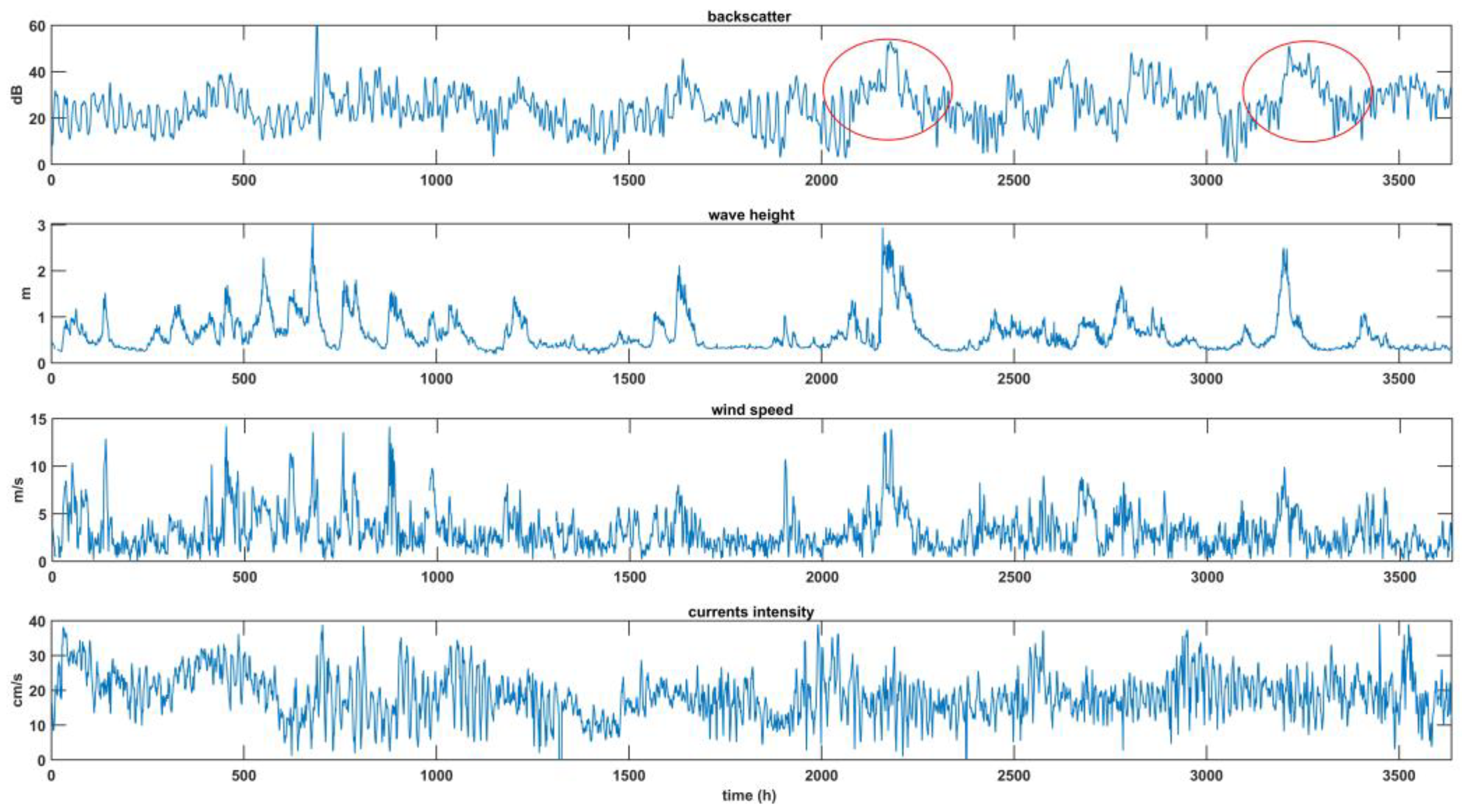
To this end, the time series of backscatter data collected from a W1-M3A system at 8 m depth were checked against concurrent Meteo-Oceanographic data provided by the same observation system (Figure 9).

The experiments took place from April to the end of August, a period generally characterized by mild and calm weather conditions and by a less intense cyclonic circulation [46,47].

Two main significant events of persistent rough sea state with waves higher than 2.5 m occurred during the examined period in a correspondence of which the backscatter increased but the amplitude of the daily oscillations, indicating the migrations, was strongly reduced, if not even hardly detected.

The wind does not seem to directly affect the acoustic signal, probably because its effect is attenuated by the 8 m depth water column.

Horizontal currents measured by the ADCP at an 8 m depth are dominated by the inertial motions; mean current intensity during the whole period is 18.5 cm/s, with some peaks up to 40 cm/s. Measurements in the layers below as well as previous investigations in the same position [47] depict a barotropic layer moving to the north-west; these currents do not have an influence on the migration patterns and no evident relation with the wind could be found.

Results indicate to also consider GIS layers with Meteo-Oceanographic data, as reported in the example of Figure 10, where wave height was displayed for each position at the time of each measurement with a color scale.

5. Discussions

Remote measurements of acoustic backscatter have become a widely used system for marine environmental monitoring [48].

The GIS application here described addressed the question of how an efficient GIS management of backscatter data obtained from moving platforms such as research and hydrographic vessels and, more recently, from the gliders can be of advantage for biological investigations. The main problem faced during the analysis of these data-sets is related to the need of combining the movements of the platform along its route with the vertical movement of the investigated organisms, in order to accurately map their spatial distribution. To this end, the capability of GIS to select the data corresponding to the different migration phases allows for a more precise determination of patches’ size and structures.

The advantage of GIS to integrate different layers is also a great help to enlighten the relation of zooplankton behavior and ecology with environmental and climatic conditions, since the system can manage layers with horizontal maps of climatological data, as well as surface maps from satellite observations and/or Essential Ocean Variables (EOV) data measured during oceanographic campaigns.

Whichever is the selected layer, by clicking on a position, the values of the parameters associated to all the other layers in that point are immediately visualized on a panel in the screen (Figure 11); moreover, the user can easily switch from one layer to another to have a view of the spatial distribution of the selected parameter.

The analysis of the backscatter data should also take into consideration the effects of local meteorological and geographic conditions that can hamper a clear data interpretation. The backscatter increase due to the sea waves was confirmed in this analysis; along the coasts, river runoff and the associated sediment transport may alter the backscatter signals. The high values detected at the exit of the Port of La Spezia (Figure 7) can be likely ascribed to the high sediment transport characterizing the area, but even the presence of high biomass [49] can contribute to the local high values. Moreover, a backscatter increase related to the rough sea cannot be excluded, as the wave height was above 1.5 m, the highest reached during that campaign.

The use of the false color technique seems to be a promising solution to visualize the horizontal distribution of the depth dependent pattern, provided that the metric defined for the characterization of the mode decomposition is of easy user interpretation. Despite this technique being validated adopting a simple scheme, random selected data were well fitted with the model, thus allowing one to expand the GIS functions to the management of the backscatter profiles. A similar processing can be also of the advantage to automatically identify “anomalies” in large data bases: an example is the higher backscatter intensity in front of Genoa Port (Figure 12), probably to be ascribed to high sediment concentration. However, the high backscatter values due to the bottom can be eliminated by integration with the layer of the bathymetry.

The results from the test case also put in to evidence some weaknesses, thus indicating the way for future developments: an important source of remote acoustic data also comes from long-term monitoring systems from fixed locations. As GIS are not devised to be used for the analysis of these data, increased effort must be made to find the best technique to integrate the time series of data from a fixed point within the system.

For the presented test case, the data collected along the route during two oceanographic campaigns were used but the limited amount of the available data did not provide an adequate spatial coverage for a horizontal gridded field representation, so that the effectiveness of some applications could not be properly proved. As the population of the database will increase, more visualizations and analysis tools will be tested. Moreover, the developed system will be extended to manage the huge amount of water column multibeam echosounder data collected by IIM for hydrographic purposes in order to give added values and make them available to support other environmental studies.

GIS has been proven to be an efficient tool for supporting analysis in the field of ecological research but the application to zooplankton distribution is a relative novel scenario in the literature. In this study, the added value consists in the merging of metadata with a geospatial component based on maps to provide insight on the migration pattern of zooplankton. GIS allowed one to analyze changes in the backscatter data due to day–night alternation in an intuitive way, without the need for the researchers to create different datasets, as, for example, being associated to night-time or day-time. Using the proposed tool, it is possible to study the zooplankton migration pattern with temporal and spatial variability of environmental conditions, which is another added value of GIS. Furthermore, GIS can provide immediate information on the different layers related to the different depths and specifically, for our study it provides information on the zooplankton distribution along the water column, that is one of the key issues for ecological studies based on indirect measurements. The added value of this tool has also been proven recently in literature [24,50,51] describing the GIS tool developed by other authors to investigate the spatial and temporal distribution of zooplankton in the surveyed areas. In these works, it is well stressed how this methodology can be useful to different specialists for understanding the patterns and drivers of zooplankton diversity and biomass variations at large scales. The same approach could also be useful for other parameters linked to backscatter data such as sediment distribution.

References

- Lavery, A.C.; Chu, D.; Moum, J.N. Measurements of Acoustic Scattering from Zooplankton and Oceanic Microstructure Using a Broadband Echosounder. ICES J. Mar. Sci. 2010, 67, 379–394. [Google Scholar] [CrossRef] [Green Version]
- Reiss, C.S.; Cossio, A.M.; Walsh, J.; Cutter, G.R.; Watters, G.M. Glider-Based Estimates of Meso-Zooplankton Biomass Density: A Fisheries Case Study on Antarctic Krill (Euphausia Superba) Around the Northern Antarctic Peninsula. Front. Mar. Sci. 2021, 8, 604043. [Google Scholar] [CrossRef]
- Johnson, J.J.; Miksis-Olds, J.L.; Lippmann, T.C.; Jech, J.M.; Seger, K.D.; Pringle, J.M.; Linder, E. Decadal Community Structure Shifts with Cold Pool Variability in the Eastern Bering Sea Shelf. J. Acoust. Soc. Am. 2022, 152, 201–213. [Google Scholar] [CrossRef] [PubMed]
- Gordon, R.L. Acoustic Doppler Current Profiler: Principles of Operation—A Practical Primer; Teledyne RD Instruments: Poway, CA, USA, 1996; p. 52. [Google Scholar]
- Schott, F.; Johns, W. Half-Year-Long Measurements with a Buoy-Mounted Acoustic Doppler Current Profiler in the Somali Current. J. Geophys. Res. 1987, 92, 5169. [Google Scholar] [CrossRef]
- Schott, F.; Leaman, K.D. Observations with Moored Acoustic Doppler Current Profilers in the Convection Regime in the Golfe Du Lion. J. Phys. Oceanogr. 1991, 21, 558–574. [Google Scholar] [CrossRef]
- Plueddemann, A.J.; Pinkel, R. Characterization of the Patterns of Diel Migration Using a Doppler Sonar. Deep Sea Research Part A. Oceanogr. Res. Pap. 1989, 36, 509–530. [Google Scholar] [CrossRef]
- Jiang, S.; Dickey, T.D.; Steinberg, D.K.; Madin, L.P. Temporal Variability of Zooplankton Biomass from ADCP Backscatter Time Series Data at the Bermuda Testbed Mooring Site. Deep Sea Res. Part I Oceanogr. Res. Pap. 2007, 54, 608–636. [Google Scholar] [CrossRef]
- Cisewski, B.; Strass, V.H.; Rhein, M.; Krägefsky, S. Seasonal Variation of Diel Vertical Migration of Zooplankton from ADCP Backscatter Time Series Data in the Lazarev Sea, Antarctica. Deep Sea Res. Part I Oceanogr. Res. Pap. 2010, 57, 78–94. [Google Scholar] [CrossRef] [Green Version]
- Potiris, E.; Frangoulis, C.; Kalampokis, A.; Ntoumas, M.; Pettas, M.; Petihakis, G.; Zervakis, V. Acoustic Doppler Current Profiler Observations of Migration Patterns of Zooplankton in the Cretan Sea. Ocean Sci. 2018, 14, 783–800. [Google Scholar] [CrossRef] [Green Version]
- Raybaud, V.; Nival, P.; Mousseau, L.; Gubanova, A.; Altukhov, D.; Khvorov, S.; Ibañez, F.; Andersen, V. Short Term Changes in Zooplankton Community during the Summer-Autumn Transition in the Open NW Mediterranean Sea: Species Composition, Abundance and Diversity. Biogeosciences 2008, 5, 1765–1782. [Google Scholar] [CrossRef]
- Ursella, L.; Pensieri, S.; Pallàs-Sanz, E.; Herzka, S.Z.; Bozzano, R.; Tenreiro, M.; Cardin, V.; Candela, J.; Sheinbaum, J. Diel, Lunar and Seasonal Vertical Migration in the Deep Western Gulf of Mexico Evidenced from a Long-Term Data Series of Acoustic Backscatter. Prog. Oceanogr. 2021, 195, 102562. [Google Scholar] [CrossRef]
- Brun, P.; Stamieszkin, K.; Visser, A.W.; Licandro, P.; Payne, M.R.; Kiørboe, T. Climate Change Has Altered Zooplankton-Fuelled Carbon Export in the North Atlantic. Nat. Ecol. Evol. 2019, 3, 416–423. [Google Scholar] [CrossRef] [PubMed] [Green Version]
- González-Gil, R.; Taboada, F.G.; Höfer, J.; Anadón, R. Winter Mixing and Coastal Upwelling Drive Long-Term Changes in Zooplankton in the Bay of Biscay (1993–2010). J. Plankton Res. 2015, 37, 337–351. [Google Scholar] [CrossRef]
- Greene, C. The Response of Calanus Finmarchicus Populations to Climate Variability in the Northwest Atlantic: Basin-Scale Forcing Associated with the North Atlantic Oscillation. ICES J. Mar. Sci. 2000, 57, 1536–1544. [Google Scholar] [CrossRef]
- Warren, J.D. Zooplankton in the Ligurian Sea: Part II. Exploration of Their Physical and Biological Forcing Functions during Summer 2000. J. Plankton Res. 2004, 26, 1419–1427. [Google Scholar] [CrossRef] [Green Version]
- Picco, P.; Schiano, M.E.; Pensieri, S.; Bozzano, R. Time-Frequency Analysis of Migrating Zooplankton in the Terra Nova Bay Polynya (Ross Sea, Antarctica). J. Mar. Syst. 2017, 166, 172–183. [Google Scholar] [CrossRef]
- Molinero, J.C.; Ibanez, F.; Souissi, S.; Chifflet, M.; Nival, P. Phenological Changes in the Northwestern Mediterranean Copepods Centropages Typicus and Temora Stylifera Linked to Climate Forcing. Oecologia 2005, 145, 640–649. [Google Scholar] [CrossRef]
- Salgado-Hernanz, P.M.; Racault, M.-F.; Font-Muñoz, J.S.; Basterretxea, G. Trends in Phytoplankton Phenology in the Mediterranean Sea Based on Ocean-Colour Remote Sensing. Remote Sens. Environ. 2019, 221, 50–64. [Google Scholar] [CrossRef]
- Fielding, S.; Griffiths, G.; Roe, H.S.J. The Biological Validation of ADCP Acoustic Backscatter through Direct Comparison with Net Samples and Model Predictions Based on Acoustic-Scattering Models. ICES J. Mar. Sci. 2004, 61, 184–200. [Google Scholar] [CrossRef] [Green Version]
- Novikov, M.A. Integrated GIS-Based Estimate of Plankton and Benthos Biomasses in the Barents Sea. Water Resour. 2008, 35, 212–219. [Google Scholar] [CrossRef]
- Wright, D. GIS for the Oceans; ESRI: Redlands, CA, USA, 2011. [Google Scholar]
- Putra, M.; Lewis, S.; Kurniasih, E.; Prabuning, D.; Faiqoh, E. Plankton Biomass Models Based on GIS and Remote Sensing Technique for Predicting Marine Megafauna Hotspots in the Solor Waters. IOP Conf. Ser.Earth Environ. Sci. 2016, 47, 012015. [Google Scholar] [CrossRef] [Green Version]
- Volvenko, I.V. Geographical Zonation in the Distribution of the Integral Characteristics of Net Zooplankton in Far Eastern Seas and in the North Pacific. Sci. Total Environ. 2020, 715, 136961. [Google Scholar] [CrossRef] [PubMed]
- Bordone, A.; Ciuffardi, T.; Raiteri, G.; Schirone, A.; Bozzano, R.; Pensieri, S.; Pennecchi, F.; Picco, P. Improved Current Estimates from Spar Buoy-Mounted ADCP Measurement Station: A Case Study in the Ligurian Sea. JMSE 2021, 9, 466. [Google Scholar] [CrossRef]
- Storto, A.; Oddo, P.; Cozzani, E.; Coelho, E.F. Introducing Along-Track Error Correlations for Altimetry Data in a Regional Ocean Prediction System. J. Atmos. Ocean. Technol. 2019, 36, 1657–1674. [Google Scholar] [CrossRef]
- Deines, K.L. Backscatter Estimation Using Broadband Acoustic Doppler Current Profilers. In Proceedings of the IEEE Sixth Working Conference on Current Measurement (Cat. No.99CH36331); IEEE: San Diego, CA, USA, 1999; pp. 249–253. [Google Scholar]
- Gostiaux, L.; van Haren, H. Extracting Meaningful Information from Uncalibrated Backscattered Echo Intensity Data. J. Atmos. Ocean. Technol. 2010, 27, 943–949. [Google Scholar] [CrossRef]
- Mullison, J. Backscatter Estimation Using Broadband Acoustic Doppler Current Profilers—Updated. In Proceedings of the ASCE Hydraulic Measurements & Experimental Methods Conference, Durham, UK, 9 July 2017; American Society of Civil Engineers: Reston, VA, USA, 2017. [Google Scholar]
- Ainslie, M.A.; McColm, J.G. A Simplified Formula for Viscous and Chemical Absorption in Sea Water. J. Acoust. Soc. Am. 1998, 103, 1671–1672. [Google Scholar] [CrossRef]
- Boucher, J.; Ibanez, F.; Prieur, L. Daily and Seasonal Variations in the Spatial Distribution of Zooplankton Populations in Relation to the Physical Structure in the Ligurian Sea Front. J. Mar. Res. 1987, 45, 133–173. [Google Scholar] [CrossRef]
- Licandro, P. Changes of Zooplankton Communities in the Gulf of Tigullio (Ligurian Sea, Western Mediterranean) from 1985 to 1995. Influence of Hydroclimatic Factors. J. Plankton Res. 2000, 22, 2225–2253. [Google Scholar] [CrossRef]
- Licandro, P.; Icardi, P. Basin scale distribution of zooplankton in the Ligurian Sea (north-western Mediterranean) in late autumn. Hydrobiologia 2009, 617, 17–40. [Google Scholar] [CrossRef]
- Tarling, G.A.; Matthews, J.B.L.; David, P.; Guerin, O.; Buchholz, F. The Swarm Dynamics of Northern Krill (Meganyctiphanes Norvegica) and Pteropods (Cavolinia Inflexa) during Vertical Migration in the Ligurian Sea Observed by an Acoustic Doppler Current Profiler. Deep Sea Res. Part I Oceanogr. Res. Pap. 2001, 48, 1671–1686. [Google Scholar] [CrossRef]
- Bozzano, R.; Fanelli, E.; Pensieri, S.; Picco, P.; Schiano, M.E. Temporal Variations of Zooplankton Biomass in the Ligurian Sea Inferred from Long Time Series of ADCP Data. Ocean Sci. 2014, 10, 93–105. [Google Scholar] [CrossRef] [Green Version]
- Guerra, D.; Schroeder, K.; Borghini, M.; Camatti, E.; Pansera, M.; Schroeder, A.; Sparnocchia, S.; Chiggiato, J. Zooplankton Diel Vertical Migration in the Corsica Channel (North-Western Mediterranean Sea) Detected by a Moored Acoustic Doppler Current Profiler. Ocean Sci. 2019, 15, 631–649. [Google Scholar] [CrossRef] [Green Version]
- Fella, A. Estimating Zooplankton Distribution from ADCP Backscatter Acoustic Analysis: Ligurian Sea Case Study. In Post Graduate Master Degree on Marine Geomatics: Advanced Technologies Applied on Marine Environment; University of the Study of Genoa: Genoa, Italy, 2022. [Google Scholar]
- Morelli, D.; Locatelli, M.; Corradi, N.; Cianfarra, P.; Crispini, L.; Federico, L.; Migeon, S. Morpho-Structural Setting of the Ligurian Sea: The Role of Structural Heritage and Neotectonic Inversion. JMSE 2022, 10, 1176. [Google Scholar] [CrossRef]
- Fanelli, E.; Delbono, I.; Ivaldi, R.; Pratellesi, M.; Cocito, S.; Peirano, A. Cold-Water Coral Madrepora Oculata in the Eastern Ligurian Sea (NW Mediterranean): Historical and Recent Findings. Aquatic. Conserv. Mar. Freshw. Ecosyst. 2017, 27, 965–975. [Google Scholar] [CrossRef]
- Pratellesi, M.; Ivaldi, R.; Delbono, I. Dual Use Hydrographic Surveys for Seabed Nature and Morphological Research. Hydro Int. 2014, 18, 26–29. [Google Scholar]
- Thomson, R.E.; Emery, W.J. Data Analysis Methods in Physical Oceanography, 3rd ed.; Elsevier: Amsterdam, The Netherlands, 2014; ISBN 978-0-12-387782-6. [Google Scholar]
- Hannachi, A. Empirical Orthogonal Functions. In Patterns Identification and Data Mining in Weather and Climate; Springer Atmospheric Sciences; Springer International Publishing: Cham, Switzerland, 2021; pp. 31–69. ISBN 978-3-030-67072-6. [Google Scholar]
- Visbeck, M.; Fischer, J. Sea Surface Conditions Remotely Sensed by Upward-Looking ADCPs. J. Atmos. Ocean. Technol. 1995, 12, 141–149. [Google Scholar] [CrossRef]
- Marmorino, G.O.; Hallock, Z.R. On Estimating Wind Velocity Using an Upward-Looking ADCP. J. Atmos. Ocean. Technol. 2001, 18, 791–798. [Google Scholar] [CrossRef]
- Wang, H.; Chen, H.; Xue, L.; Liu, N.; Liu, Y. Zooplankton Diel Vertical Migration and Influence of Upwelling on the Biomass in the Chukchi Sea during Summer. Acta Oceanol. Sin. 2015, 34, 68–74. [Google Scholar] [CrossRef]
- Prieur, L.; D’Ortenzio, F.; Taillandier, V.; Testor, P. Physical Oceanography of the Ligurian Sea. In The Mediterranean Sea in the Era of Global Change 1; Migon, C., Nival, P., Sciandra, A., Eds.; Wiley: New York, NY, USA, 2020; pp. 49–78. ISBN 978-1-78630-428-5. [Google Scholar]
- Picco, P.; Cappelletti, A.; Sparnocchia, S.; Schiano, M.E.; Pensieri, S.; Bozzano, R. Upper Layer Current Variability in the Central Ligurian Sea. Ocean Sci. 2010, 6, 825–836. [Google Scholar] [CrossRef] [Green Version]
- Colbo, K.; Ross, T.; Brown, C.; Weber, T. A Review of Oceanographic Applications of Water Column Data from Multibeam Echosounders. Estuar. Coast. Shelf Sci. 2014, 145, 41–56. [Google Scholar] [CrossRef]
- Gasparini, G.P.; Abbate, M.; Bordone, A.; Cerrati, G.; Galli, C.; Lazzoni, E.; Negri, A. Circulation and Biomass Distribution during Warm Season in the Gulf of La Spezia (North-Western Mediterranean). J. Mar. Syst. 2009, 78, S48–S62. [Google Scholar] [CrossRef]
- Canencia, M.O.P.; Ascaño, C.P. Marine Zooplankton Distribution Model and Seriation Index across Different Habitat Types. Int. J. Res. Appl. Sci. Eng. Technol. (IJRASET) 2017, 5, 1646–1652. [Google Scholar] [CrossRef]
- Ismail, A.H.; Rahman, A.A.; Chin, L.C. The Use of GIS to Visualize Spatial Distribution of Zooplankton in Teluk Bahang Reservoir, Penang, Malaysia. J. Environ. Sci. Manag. 2020, 23, 60–71. [Google Scholar] [CrossRef]