Effects of Strain-Softening and Strain-Rate Dependence on the Anchor Dragging Simulation of Clay through Large Deformation Finite Element Analysis

Abstract

Large-deformation finite element (LDFE) analysis with the coupled Eulerian–Lagrangian (CEL) technique for large-deformation soil functions without twisting or distorting the mesh. However, the model does not consider the strain-softening and strain-rate dependence of clay-based soils. The undrained shear strength of clay is sensitive to the strain rate. In addition, the strain-softening effect of soil strength reduction accompanied by large-scale shear deformation should be considered. In this study, anchor dragging simulations were performed for large-deformation analysis considering strain-softening and strain-rate dependence. Furthermore, a shear strength equation expressing the strain-softening and strain-rate dependence of the Tresca constitutive model was developed based on VUMAT, an ABAQUS/Explicit subroutine. The equation was designed so that it could be linked to the LDFE/CEL model. The model was verified by performing comparative analysis with the Mohr–Coulomb (M–C) perfect-plasticity model. The newly constructed Tresca base strain-softening and strain-rate-dependence VUMAT algorithm in the LDFE/CEL model analysis confirmed the effects of strain-softening and strain-rate dependence. The proposed model enabled a highly realistic simulation of the actual phenomenon than the M–C model. Finally, a parametric study on strain-softening and strain-rate dependence was conducted, and the behavior of clay due to the anchor drag phenomenon was revealed.

1. Introduction

Finite element analysis (FEA) is an important tool for material behavioral simulation and analysis in disciples such as civil engineering, where it is used to examine the soil-structure interaction. However, simulations of the behavior of terrain composed of clay, such as the seabed, experience severe mesh distortions and contact problems owing to excessive deformation. Consequently, the accuracy and convergence of the analysis are degraded [1]. Efforts to solve this problem include applying large-deformation finite element (LDFE) analysis to various cases involving large-deformation soil.

A typical method utilized in LDFE analysis is the coupled Eulerian–Lagrangian (CEL) technique, which combines Lagrangian and Eulerian simulations for the large deformation of the anchor and the relatively small deformation of the soil together by defining the continuum behavior as the coordinates and time of the object. The behavior of Lagrangian elements in the region simulated by Eulerian is expressed as EVF (Eulerian volume fraction), which is the volume ratio of each element as depicted in Figure 1, each Eulerian element is expressed as a ratio of physical properties, and an analysis has been conducted without twisting or distorting the mesh.

The LDFE/CEL model technique has been applied to various soils composed of clay. Simulations of the penetration and dragging of ship anchors [2,3] and studies on the penetration depth of OMNI-Max and Torpedo anchors [4,5,6] have also been performed. An investigation comparing three methods (the Implicit, Explicit, and CEL methods) was conducted for the pile installation problem [7]. In addition, various studies on the effects of horizontal pullout on plate anchors under large-deformation conditions have been conducted [8,9,10,11].

The behavior of caissons resulting from soil uplift [12] and the cone penetration test [13] have also been simulated using the CEL technique. In particular, a numerical simulation method for anchor dragging has been applied to the analysis of the LDFE/CEL model and is being actively studied [14,15].

However, studies in which anchor drag has been simulated have not considered the strain-softening or strain-rate dependence of clay soils. In general, the undrained shear strength of clay is sensitive to the strain rate. The softening effect of ground strength reduction accompanied by large-scale shear deformation (herein, referred to as large deformation) should also be considered. According to previous studies, the softening effect negates the increase in strength due to the strain rate [4]. However, these complex effects significantly vary with the type and sensitivity of the clay soil. Moreover, this effect decreases as the soil becomes sandy [16]. Accordingly, to simulate the LDFE/CEL model analysis of large-deformation clay and, by extension, the anchor drag, the complex effects of strain-softening and strain-rate dependence must be considered.

Therefore, in this study, anchor drag was simulated by performing LDFE/CEL model analysis considering the strain-softening and strain-rate dependence. To this end, a return mapping algorithm based on the Tresca constitutive model was defined [17] and an ABAQUS user subroutine was created to consider the strain-softening and strain-rate dependence on the anchored ground. The subroutine was reflected in VUMAT [18]. In addition, the shear strength equation considering the strain-softening and strain-rate dependence, proposed by Einav and Randolph [19], and formalized by Zhou and Randolph [20], was modified for use in VUMAT, in conjunction with the return mapping algorithm. By applying VUMAT to the basic soil behavior problem, we verified its consistency. This step was preceded by a comparative analysis of the mentioned equation with the Mohr–Coulomb (M–C) model, which does not consider strain-softening or strain-rate dependence. To examine the effects of the strain-softening and strain-rate dependence, cases were classified, analyzed, and compared. Based on the results, the LDFE/CEL model was reflected and applied to the ship-anchor drag scenario to analyze the soil behavior resulting from anchor dragging. Finally, a parametric study was performed on the parameters applied in the simulation to reveal the behavior of clay due to the anchor drag phenomenon.

2. Implementation of Soil Constitutive Models

2.1. Failure Criterion

The Tresca yield occurs when the maximum shear stress generated in the material reaches a specific critical value (Figure 2a) and can be expressed as:

$${\tau }_{max}=max\left\{\frac{1}{2}\left|{\sigma }_1-{\sigma }_2\right|,\frac{1}{2}\left|{\sigma }_2-{\sigma }_3\right|,\frac{1}{2}\left|{\sigma }_3-{\sigma }_1\right|\right\}=k.$$

(1)

The Tresca model yield criterion, which is the most common yield criterion for various materials, is independent of hydrostatic pressure. In this criterion, the yield surface is a regular hexagonal column in the diagonal spatial direction, with the center on the diagonal spatial line. In addition, the yield criterion for the M–C model, an extension of the Tresca model yield criterion, is depicted in Figure 2b and is based on the following equation:

$${\tau }_u=c+{\sigma }_n\mathit{tan}\varphi ,$$

(2)

where $c$ and $\varphi$ are the cohesive and internal friction angles, respectively, and ${\tau }_u$ and ${\sigma }_n$ are the mean shear and normal stresses acting on the fracture surface, respectively. When $\varphi =0$ and $c=k$, the M–C model yield criterion transforms into the Tresca model yield criterion. The failure criteria in the principal stress space of the M–C and Tresca models are depicted in Figure 2.

In this study, the more simplified Tresca model yield criterion was applied for terrain composed of clay.

2.2. General Stress Return Mapping Algorithm

The basic concept of plasticity is that, when the material yields, the yield function becomes 0:

$$f\left(\sigma \right)=0,$$

(3)

where $\mathsf{\sigma }$ is the stress tensor expressed as a matrix. The elements constituting the stress and strain can be expressed as:

$$\sigma ={\left[{\sigma }_x{\sigma }_y{\sigma }_z{\tau }_{xy}{\tau }_{xz}{\tau }_{yz}\right]}^T,\epsilon ={\left[{\epsilon }_x{\epsilon }_y{\epsilon }_{z}2{\epsilon }_{xy}2{\epsilon }_{xz}2{\epsilon }_{yz}\right]}^T.$$

(4)

The flow rule can be used to express the plastic strain increment as follows:

$$d{\epsilon }^P=d\lambda \frac{\partial f}{\partial \sigma }.$$

(5)

In the elasto-plastic analysis, using the finite element method, the load increment was applied incrementally, and the stress increment was updated within each displacement increment as follows:

$$\Delta \sigma ={{\displaystyle \int }}_{{\epsilon }_j}^{{\epsilon }_j+\Delta \epsilon }{D}^{ep}\left(\sigma \right)d\epsilon ,$$

(6)

where $\Delta \mathsf{\sigma }$ is the finite stress increment, ${\epsilon }_j$ is the total strain after increment $j$, and $D^{ep}\left(\sigma \right)$ is the infinitesimal elasto-plastic constituent matrix that varies with the current stress state. As $D^{ep}\left(\sigma \right)$ shares a strong non-linear relationship with $\Delta \sigma$, the approximate solution of the strain increment for Equation (6) is generally used. In addition, the basic assumption of the return mapping algorithm with a small strain is that the increase in strain is contributed in the order of elasticity and plasticity, as follows:

$$d\epsilon =d{\epsilon }^e+d{\epsilon }^p,$$

(7)

where the elastic stress increments can be derived from Hooke’s Law.

$$d\sigma =D^{e}d{\epsilon }^e=D^e\left(d\epsilon -d{\epsilon }^p\right),$$

(8)

where $D^e$ is a linear elastic isotropic tensor, and rewriting Equations (5) and (6) gives:

$$d\sigma =D^{e}d\epsilon -d\lambda D^e\frac{\partial f}{\partial \sigma }.$$

(9)

The finite stress increment $\Delta \sigma$ was calculated by integrating Equation (9), and the return mapping principle in Figure 3 can be defined as follows:

$${\sigma }^C={\sigma }^B-\Delta {\sigma }^p,$$

(10)

where $\Delta {\sigma }^e=D^e\Delta \epsilon$ and $\Delta {\sigma }^p$ are called the elastic predictor increment and plastic corrector increment, respectively. The concept of the return mapping algorithm reflects the radial return mapping algorithm proposed by Wilkins [21] and Maenchen and Sack [22] for application to the von Mises yield criterion. In their expression, the stress is first updated under the assumption that the material is elastic, where, if the elastic trial stress is outside the yield surface, it is projected to the nearest point on the yield surface (stress return).

This stress return ensures that the updated stress does not violate the yield condition, and the separation of the strain increment into elastic and plastic components is consistent with the final stress state. This system is illustrated in Figure 3. The return mapping algorithm can be evaluated using the following equation:

$$\Delta {\sigma }^p=\Delta \lambda D^{ep}{\left.\frac{\partial f}{\partial \sigma }\right|}_p,$$

(11)

where the trial principal stresses ${\sigma }_P^B$ can be calculated from ${\sigma }^B$ in Equation (10), along with the transformation matrix N through the analysis program, ABAQUS subroutine, and can be expressed as follows:

$${\sigma }_p^B=N{\sigma }^B.$$

(12)

In this study, the Tresca model yield criterion applied to clay included only the linear function of the principal stress. The corresponding yield surface at the principal stress location took the form of a line ${\sigma }_1={\sigma }_2={\sigma }_3$ and a hexagonal prism and was defined by six linear yield functions as follows:

$$\begin{gathered} f_1\left(\sigma ,s_u\right)={\sigma }_1-{\sigma }_2-2s_u, f_2\left(\sigma ,s_u\right)={\sigma }_2-{\sigma }_1-2s_u, \\ {f}_3\left(\sigma ,s_u\right)={\sigma }_2-{\sigma }_3-2s_u, f_4\left(\sigma ,s_u\right)={\sigma }_3-{\sigma }_2-2s_u, \\ {f}_5\left(\sigma ,s_u\right)={\sigma }_3-{\sigma }_1-2s_u,f_6\left(\sigma ,s_u\right)={\sigma }_1-{\sigma }_3-2s_u. \end{gathered}$$

(13)

As illustrated in Figure 4 [18], $f_{\mathrm{i}}\left(\sigma ,s_u\right)$ corresponds to surface $S_{\mathrm{i}}$ of the principal stress space, indicated as a boundary plane for the stress region of the Tresca yield criterion. In addition, the stress region related to each boundary surface $S_{\mathrm{i}}$ can be expressed by a pair of planes perpendicular to the lines at the two edges. The boundary of the stress region related to each line $L_{ij}$ passes through a line perpendicular to the two boundary surfaces $S_{\mathrm{i}}$ intersecting along the corresponding line. It is bound by two planes on which the trial principal stress ${\sigma }_p^B$ is calculated by Equation (12). It is located within the stress interface expressed in Figure 4 and returned by the return technique as a plane or line to obtain ${\sigma }_p^C$. Then, ${\sigma }^C$ in Equation (10), which is returned to the ABAQUS program, can be obtained from ${\sigma }^C=N^{-1}{\sigma }_p^C$ by using the transformation matrix N.

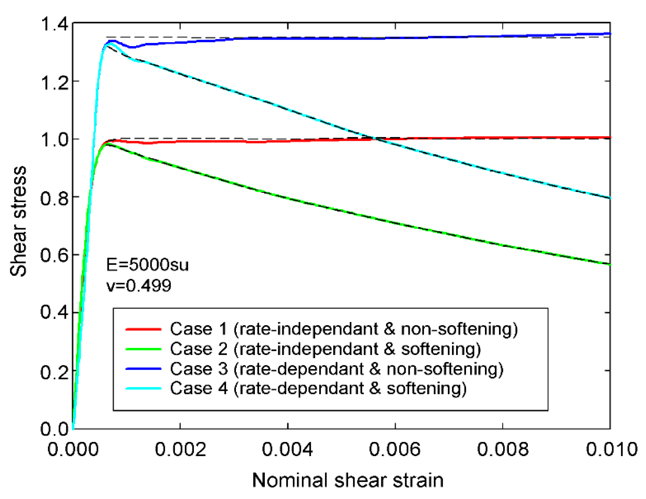
2.3. Strain-Softening and Strain-Rate Dependence

The effects of the strain softening and strain rate on the shear strength of the soil were implemented in the ABAQUS subroutine VUMAT by modifying the Tresca material using Equation (14) as follows [19,20]:

$$\begin{gathered} S_u=S_u{}_0\left[{\delta }_{rem}+\left(1-{\delta }_{rem}\right)e^{-\frac{3\xi }{{\xi }_{95}}}\right] \\ \left[1+\mu \log (\frac{\max \left({\dot{\gamma }}_{max},{\dot{\gamma }}_{ref}\right)}{{\dot{\gamma }}_{ref}}) \right], \end{gathered}$$

(14)

where $S_u$ is the shear strength of the soil, $S_u{}_0$ is the initial shear strength of the soil, $\xi$ is the plastic shear strain, and ${\delta }_{rem}$ is the reciprocal of the sensitivity of the soil $S_t$. Furthermore, $\dot{\gamma }$ is the shear strain and $\mu$ is the viscosity parameter of the soil. In Equation (14), ${\delta }_{rem}$, ${\xi }_{95}$, $\mu$, and ${\dot{\gamma }}_{ref}$ are constants related to the soil properties and were input as fixed values at the start of the analysis. A more detailed analysis will be provided in Section 5. In addition, the plastic shear strain $\xi$ and the maximum shear strain ${\dot{\gamma }}_{max}$ were calculated using the VUMAT algorithm and set to “continuously update” according to the analysis time.

In addition, the accumulated $\xi$ was stored by applying the solution-dependent variables (SDVs) that can be used in the VUMAT algorithm. Whenever VUMAT was linked in the Abaqus main program, the incremental strain $d\epsilon$ to be imposed by the current time increment was determined by searching for $\xi$ at the beginning of the time increment; this value is expressed as ${\xi }_t$. Here, the virtual strain rate $\dot{{\epsilon }^{\prime }}$ was calculated using $\dot{{\epsilon }^{\prime }}=d\epsilon /dt$, and $dt$ was employed to update the analysis model with time increments. In addition, the virtual loading rate utilized in the simulation is not necessarily the same as the actual simulation speed, because the rate of change of speed was set to be gradual to implement the static problem.

Therefore, it is necessary to introduce a scale factor $S_F$ to correct $\dot{{\epsilon }^{\prime }}$ with respect to the actual strain $\dot{\epsilon }$ by using the equation $\dot{\epsilon }=S_F\dot{{\epsilon }^{\prime }}$. The loading speed is $\nu$, and in the case of the loading process wherein the simulation loading speed is ${\nu }^{\prime }$, $S_F=\nu /\nu ’$. This scaling factor was defined as a material property, together with other parameters ($S_t$, ${\xi }_{95}$, etc.) and was input into the Abaqus/Explicit program and transmitted to the subroutine VUMAT. Moreover, when $\dot{\epsilon }$ was obtained, the maximum shear strain ${\dot{\gamma }}_{max}$ for Equation (14) could be calculated as $\dot{{\epsilon }_1}-\dot{{\epsilon }_3}$, and the currently applicable shear strength of the material was derived based on $\xi$ and ${\dot{\gamma }}_{max}$. Subsequently, VUMAT was matched with the yield condition of the material, and the stress in Figure 4 was returned with the yield surface. If the material yielded, all incremental strains used were considered plastic strains, and the cumulative plastic shear strains were calculated and updated as follows:

$${\xi }_{t+dt}={\xi }_t+\left({\dot{\epsilon }}_1-{\dot{\epsilon }}_3\right)dt,$$

(15)

where ${\xi }_{t+dt}$ is the plastic shear strain at the last time increment. The updated ${\xi }_{t+dt}$ is stored in VUMAT by the SDVs and is used to calculate the shear strength at the next time increment. As the elastic strain is a significantly small fraction (typically 0.002) compared with the plastic strain after yielding of the material, the problem of inaccuracy in the large deformation soil analysis performed in this study was excluded.

Thus, the contents implemented by the return mapping algorithm and the ABAQUS subroutine VUMAT in this study were based on the early research of Hazell (2008) [24] and Kong (2015) [23]. A new version of VUMAT was developed and applied in this study so that each variable could be incorporated into the defined algorithm by matching it with Equation (14), reflecting the dependency. The developed VUMAT version was implemented in ABAQUS to enable LDFE/CEL model analysis by adding a geotechnical concept to simulate the large-deformation ground in further detail. The technical name for the model that integrates the algorithm and large deformation analysis is the Tresca base strain-softening and strain-rate dependence (TBSR)–VUMAT model.

3. Verification of the TBSR–VUMAT Model

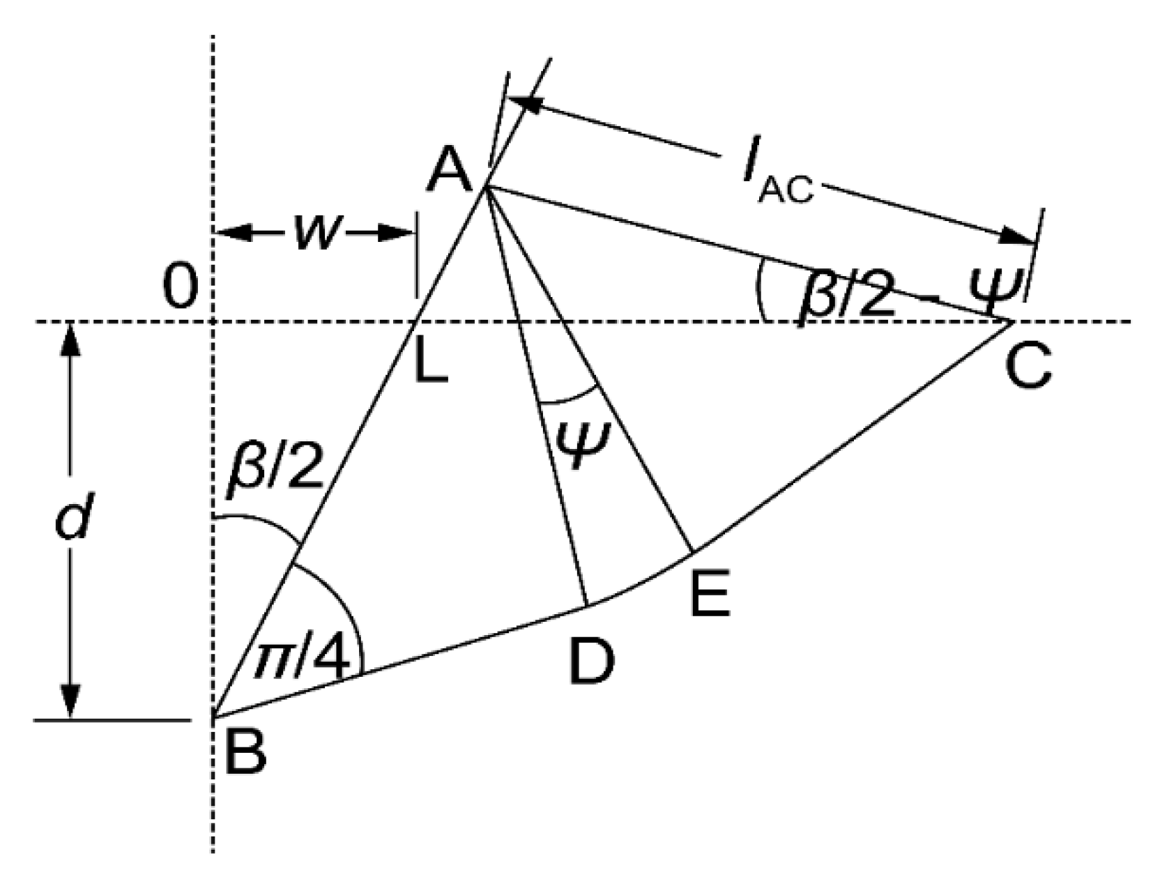
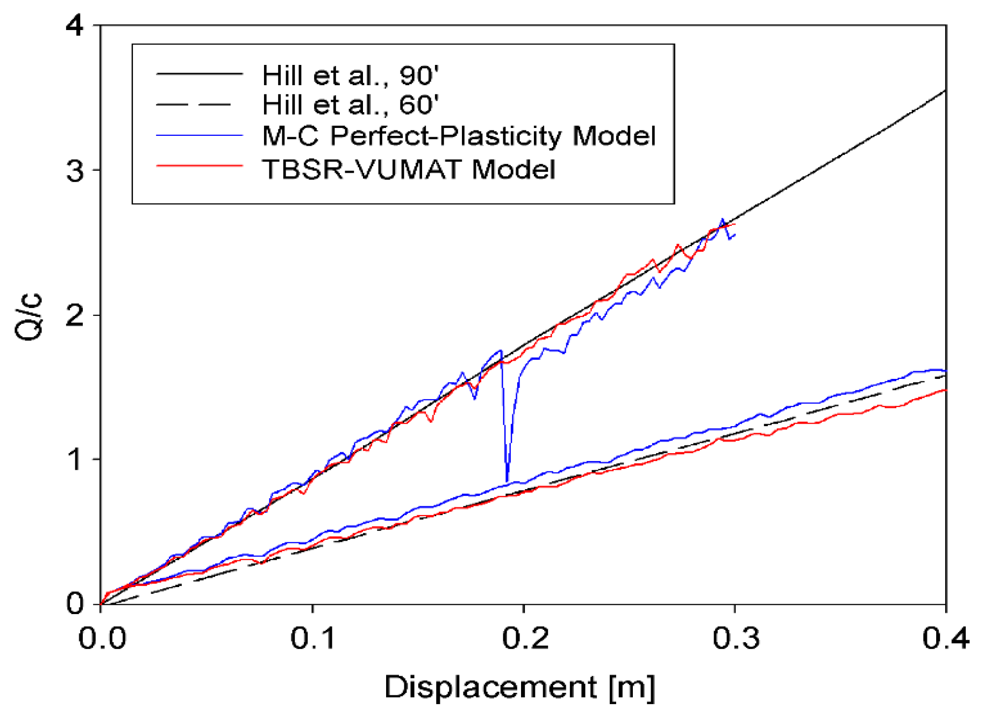
3.1. Effects on Failure Mechanisms

The developed algorithm was verified by examining the TBSR–VUMAT algorithm and comparing the results with those of Kong [24]. First, only the strain-softening- and strain-rate-dependence effects in the TBSR–VUMAT algorithm were verified, without considering large deformations, i.e., the LDFE/CEL model. For this purpose, the analysis and numerical results were compared after entering the variables in Equation (14) for the load response analysis of individual elements under pure shear stress. A model (C3D8R) composed of eight-node elements in the form of a regular hexagon with dimensions of 1 m $\times$ 1 m $\times$ 1 m was derived from the comparative model. A speed of 0.01 m/s was applied in the x-direction from the upper part of the model, and the bottom surface was fixed.

Four types of TBSR–VUMAT models were considered: non-softening and rate-independent soil (Case 1, ideal soil); softening and rate-independent soil (Case 2); non-softening and rate-dependent soil (Case 3); and softening and rate-dependent soil (Case 4).

Table 1. Strain-rate and strain-softening parameters.

	Strain Rate	Strain Softening
	µ	${\mathsf{\delta }}_{\mathit{r}\mathit{e}\mathit{m}}$	${\mathsf{\xi }}_{95}$
Case 1	0	1	1
Case 2	0	0.01	0.05
Case 3	0.1	1	1
Case 4	0.1	0.01	0.05

summarizes the parameters for each case, and Figure 5 compares the results of these cases with those of Kong (2015). The results indicated by the dotted line in Figure 5 agree with the numerical analysis results (from Equation (14)) represented by the solid line. Furthermore, the TBSR–VUMAT algorithm realistically reflects the strain-softening and strain-rate dependence.

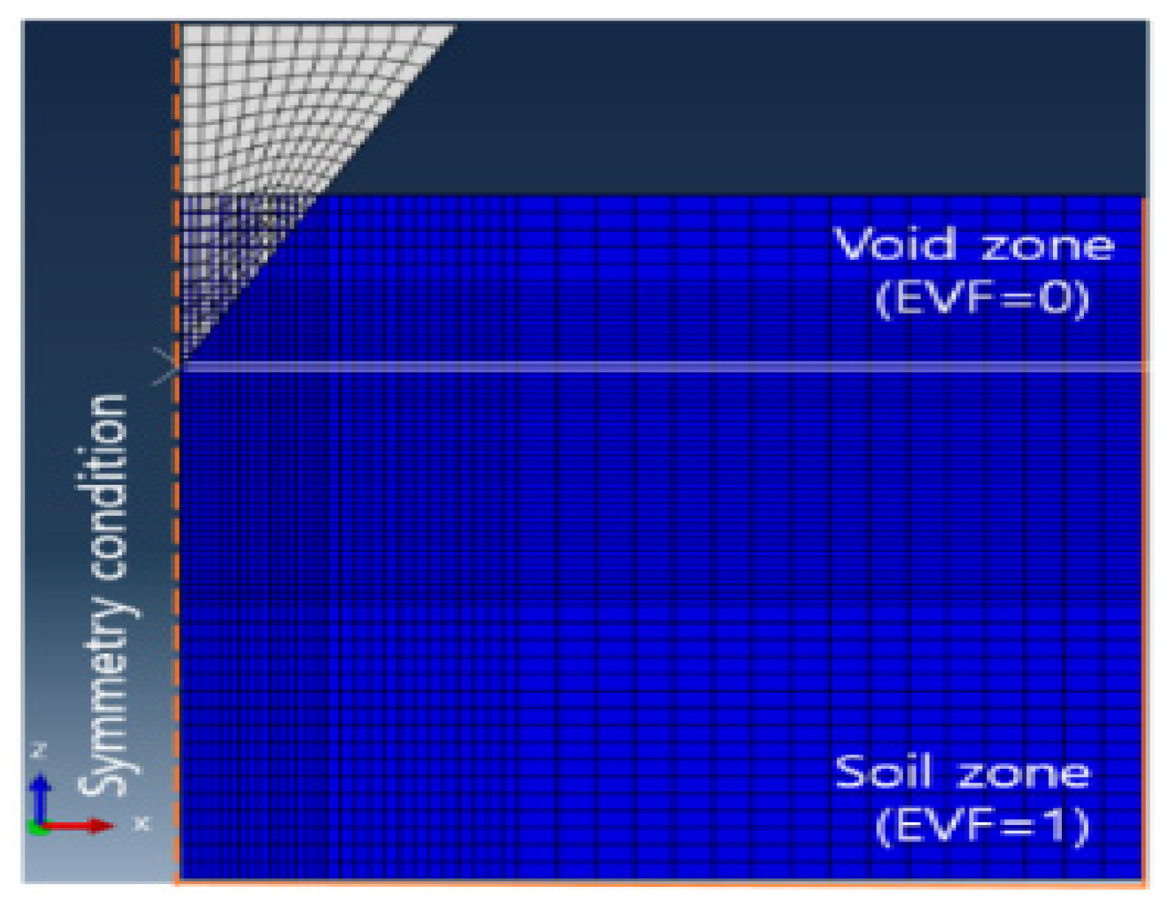
3.2. Validation of the TBSR–VUMAT Algorithm in the LDFE/CEL Model

For the second verification, an indentation test on a smooth wedge formed by a rigid body, as described by Hill et al. (1945), was applied, and the large deformations reflecting the LDFE/CEL and TBSR–VUMAT models were applied simultaneously. The analysis results were compared with those of the M–C model. The research mechanism of Hill et al. (1945) is illustrated in Figure 6. The mechanism was defined by the penetration angle and soil resistance, i.e., penetration force, in Equations (16) and (17):

$$\mathit{cos}\left(\beta -\psi \right)=\frac{cos\psi }{1+cos\psi },$$

(16)

$$Q=2p{l}_{AC}sin\frac{\beta }{2}=4c{l}_{AC}\left(1+\psi \right)sin\frac{\beta }{2}.$$

(17)

The LDFE/CEL technique was applied in the FEA model for the equations and comparisons. The model with eight nodes (EC3D8R) was constructed to model the ground. The Eulerian element was briefly introduced in Section 1. In addition, the symmetry condition was applied, and the parameters of the wedge were restrained in all directions except for the z-direction so that displacement could occur only in that direction. The wedge had a shape with angles of $60°$ and $90°$ ($\beta$/2), which could penetrate to depths of 0.4 m and 0.3 m, respectively. The topography of the entire analysis model is illustrated in Figure 7.

For the ground, a density of 0.1 $\mathrm{kg}/{\mathrm{m}}^3$, as in the work of Hill et al. [25], Young’s modulus E of 400c, and Poisson’s ratio $\upsilon$ of 0.499 were applied. Here, c is the shear strength of the ground, which was assumed to be 1 kPa. As discussed in this section, the results of the TBSR–VUMAT model to which the LDFE/CEL technique was applied and the existing M–C model with perfect plasticity as well as strain-softening and strain-rate dependence were compared. As observed in Figure 8, the results of the M–C and TBSR–VUMAT models are generally similar to those obtained by Hill et al. [25].

However, when $\beta$ is $90°$ in the M–C model, the results are marginally unstable and the error is large. Therefore, the TBSR–VUMAT model produces better results in large-deformation soil, i.e., results are slightly larger than those obtained when $\beta$ is $60°$. Therefore, the TBSR–VUMAT model algorithm used in this study accurately expresses the strain-softening- and strain-rate-dependence effects of clay. A comparison between the proposed model and the M–C model widely applied in the geotechnical field revealed that the proposed model can accurately simulate large deformation soil and yields more stable analysis results.

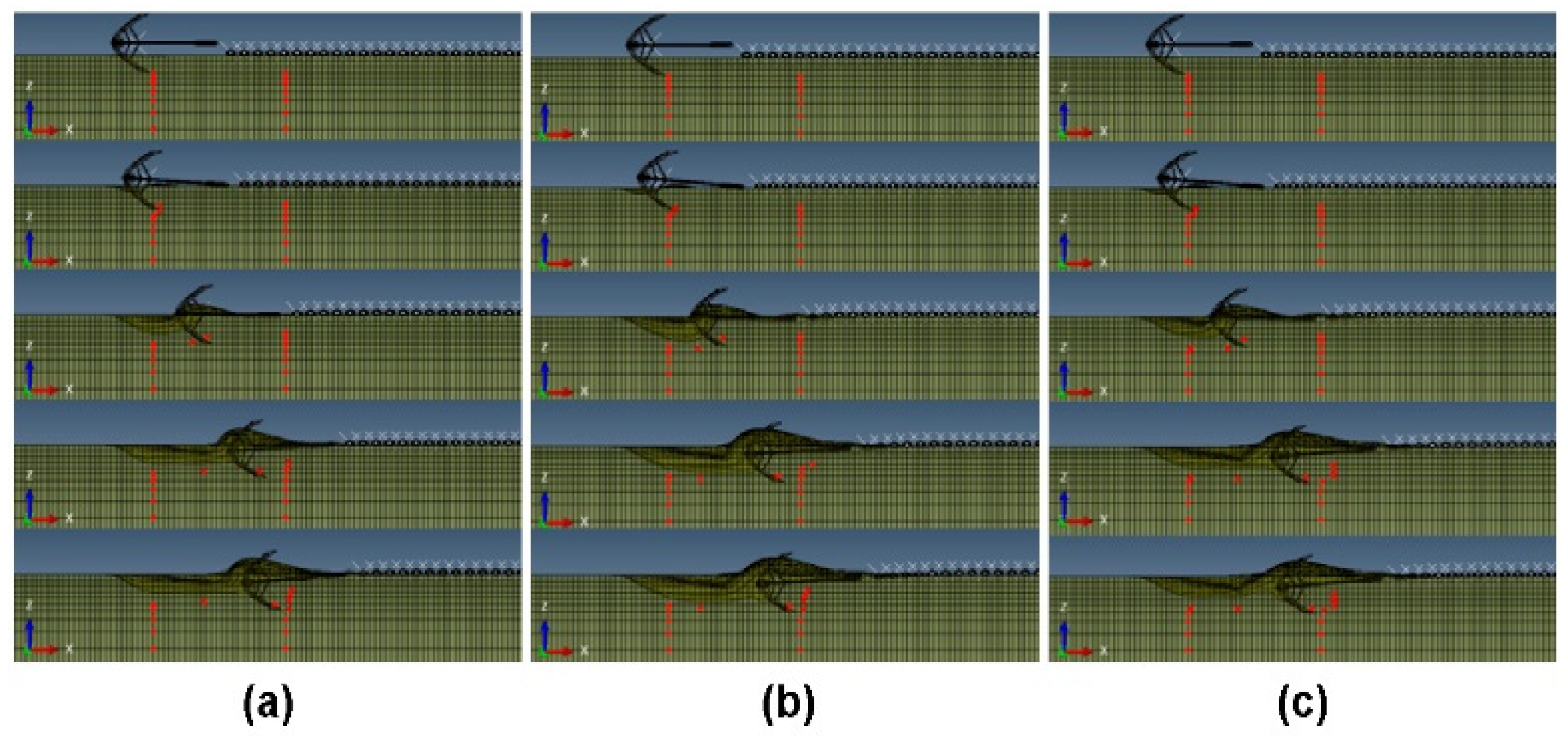
4. Anchor Dragging Simulation with TBSR–VUMAT Model

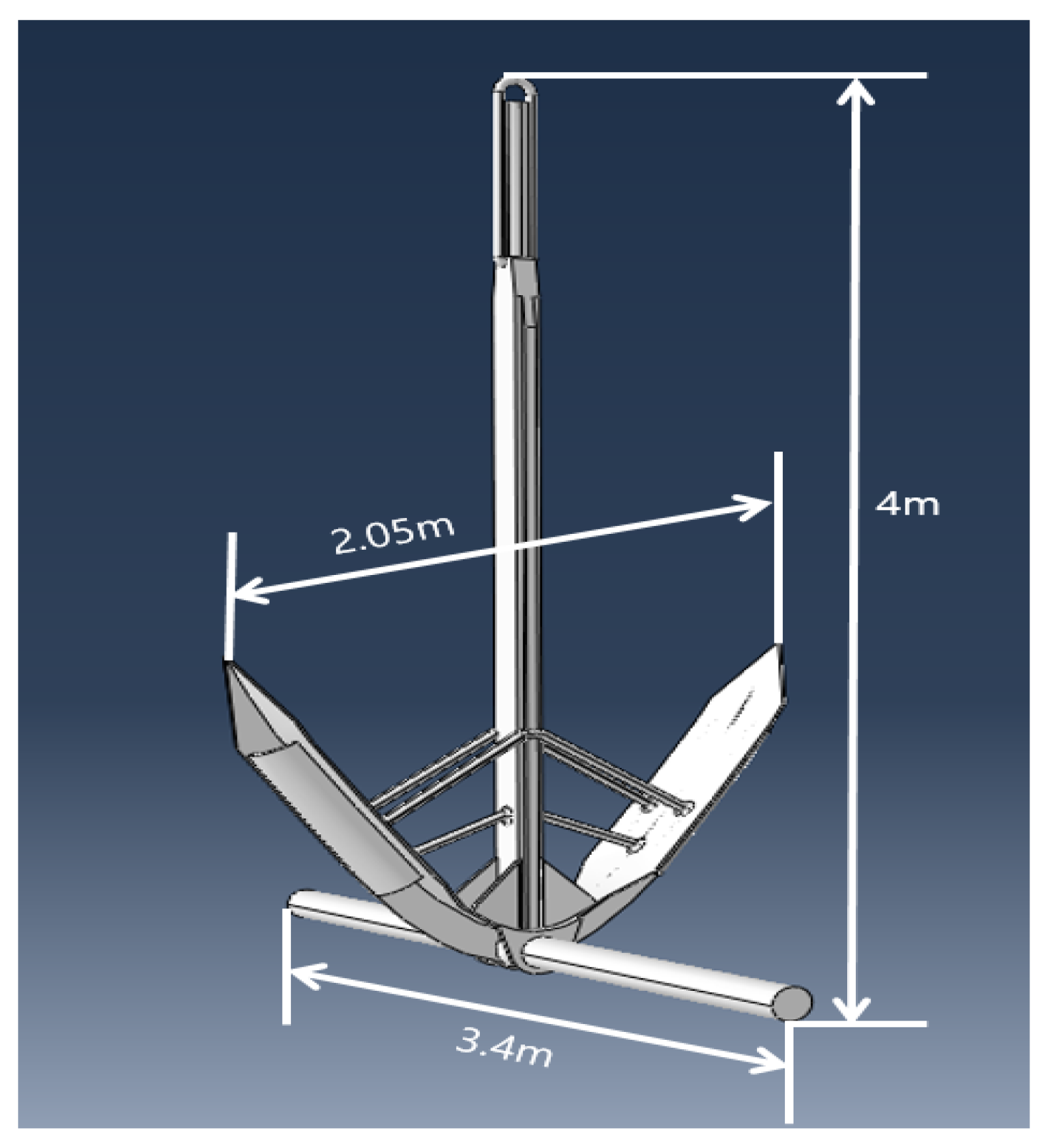
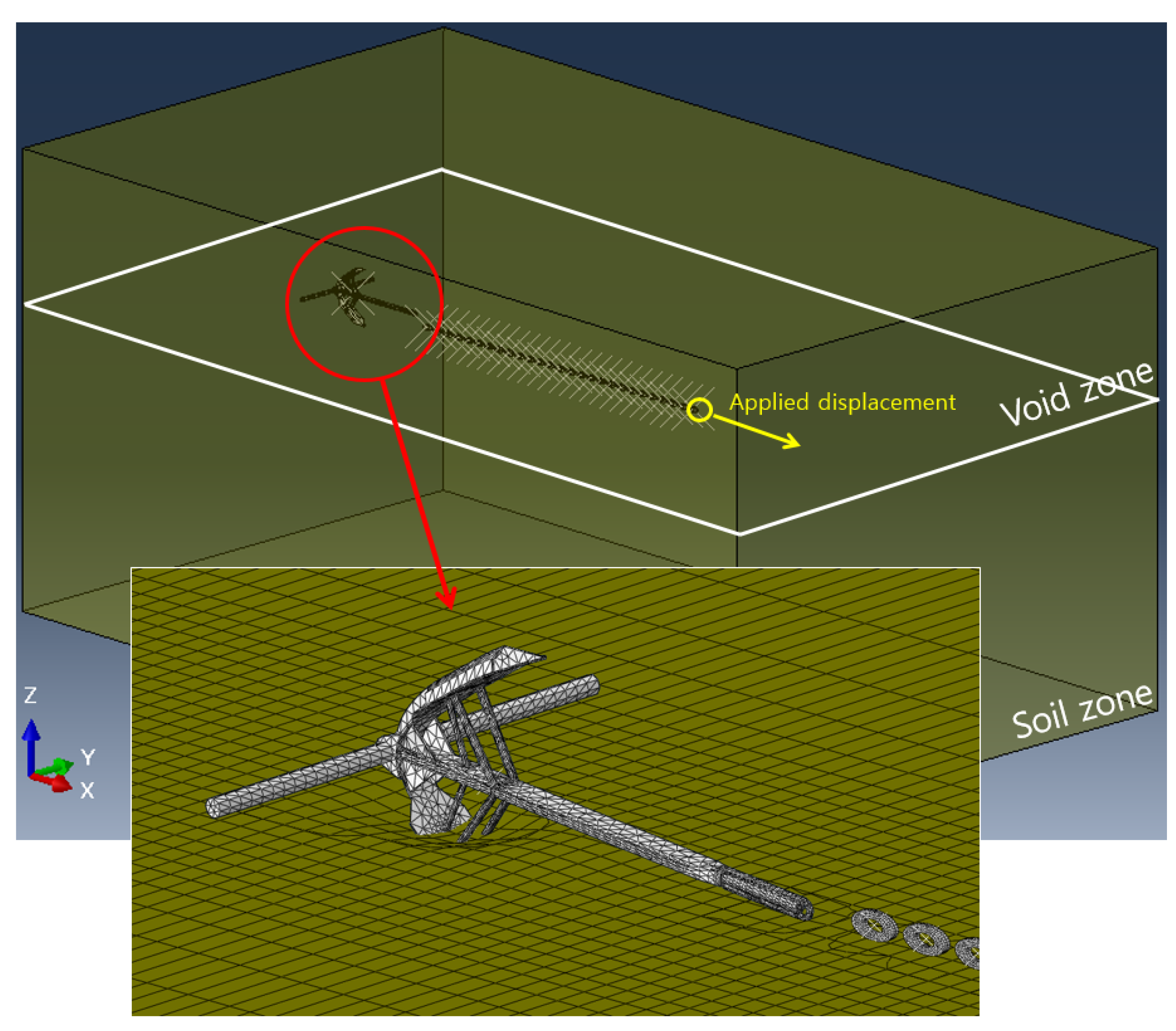
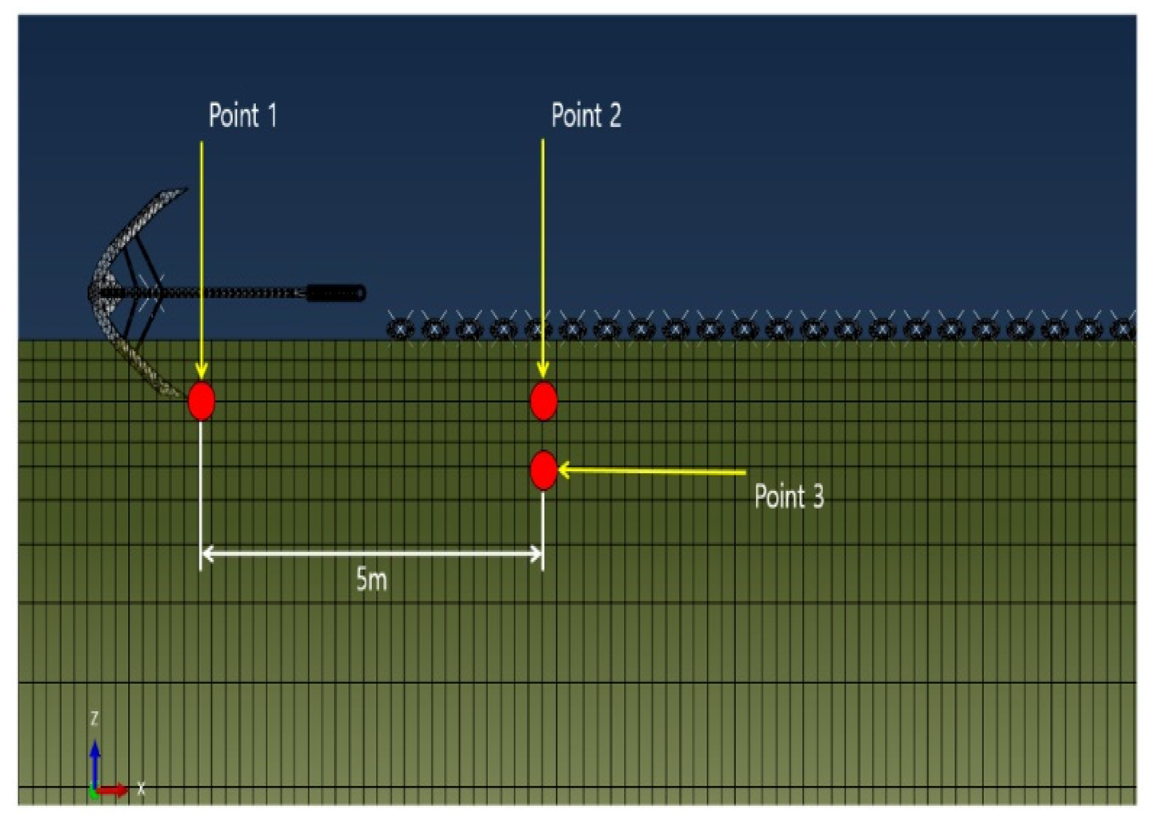
4.1. Description of the Numerical Model

The most prominent examples of LDFE/CEL model analysis include analyses of the effects of the seabed penetration depth, Torpedo anchor, and Spudcan fall [26]. Referring to the study by Shin et al. [3], in which a stow net anchor (AnGangMang, AGM anchor) used to anchor operating ships and fishing vessels was considered, the large deformation soil effect caused by drag after falling, instead of penetration by fall, was analyzed in this study. To this end, the LDFE/CEL model was applied first. As indicated in Figure 9, the AGM anchor was assumed to be a rigid body with a weight of 700 kg. The dimensions of the applied anchor are shown in Figure 9.

In addition, the model anchor was connected to a chain at its end and set to emulate the actual motion of an anchor using the weight and drag force without constraining its rotation. Similarly, the chain was set as a rigid body to control the rotation of the X- and Z-axes of the connecting part by connecting the anchor, chain, and the link-type wire connecting the chain. Displacement was applied to the last chain modeled as an anchor chain, and it was set to occur gently according to the step with the Smooth Step setting. In addition, as illustrated in Figure 10, the anchor and anchor chain were placed on the ground modeled using the LDFE/CEL approach. The model was separated into a soil zone and void zone. The number of meshes used in the FEA was 179,854, and the number of nodes was 188,209.

The boundary condition of the soil was imposed to constrain the displacements of both the bottom and side parts. In addition, the soil was modeled inside the initial Eulerian domain to impart physical properties. The boundary conditions were applied to each surface, together with the geostatic stress conditions. Geostatic stress was used to help create an initial soil more similar to the actual soil and was applied up to the final step. The equation for the geostatic stress implemented in ABAQUS was applied as the total stress of the soil and was expressed as:

$${\sigma }_v={\sigma }_v^{’}+u={\gamma }_{sat}·z.$$

(18)

In Equation (18), ${\sigma }_v$ is the total stress of the soil, ${\sigma }_v^{’}$ is the effective stress, $u$ is the pore pressure, ${\gamma }_{sat}$ is the saturated unit weight of the soil, and $z$ is the soil depth. After all the initial ground settings were implemented, displacement was applied to the anchor chain, after which the anchor was drawn.

Table 2. Material properties of the M–C model.

	$\mathit{E}$ (kPa)	$\mathsf{\upsilon }$	${\mathsf{\gamma }}_{\mathit{s}\mathit{a}\mathit{t}}$ (kg/m3)	$\mathsf{\varphi }$ $(°)$	c (kPa)
Clay	1600	0.49	1611	0.01	5.9

and

Table 3. Material properties of soil in the TBSR–VUMAT model.

	$\mathit{E}$ (kPa)	$\mathsf{\upsilon }$	$$\begin{gathered} {\mathit{S}}_{\mathit{u}} \\ \left(\mathbf{kPa}\right) \end{gathered}$$	$\mathit{k}$ (kPa/m)	${\mathsf{\delta }}_{\mathit{r}\mathit{e}\mathit{m}}$	${\mathsf{\xi }}_{95}$	$\mathsf{\mu }$	Amp
Clay	1600	0.49	2.3	3.6	0.3	20	0.1	1

list the material parameters applied to the ground.

The physical properties of the clay in the M–C model were sourced from Das [27], and the parameters applied in the TBSR–VUMAT model were obtained from Dingle et al. [28]. The values of the parameters were known and used to simulate the clay soil.

A Coulomb friction model based on the shear friction model was applied to consider the effects of friction between the anchor and soil and between the soils. If the frictional stress (${\tau }_{eq}$) defined in Equations (19) and (20) is smaller than the critical stress (${\tau }_{crit}$), then no relative motion occurs; when they are equal, slip occurs [18]:

$${\tau }_{eq}=\sqrt{{\tau }_1^2+{\tau }_2^2},$$

(19)

$${\tau }_{crit}=\mu p,$$

(20)

where ${\tau }_1$ and ${\tau }_2$ are the shear stresses at the contact surface, $\mu$ is the friction coefficient, and $p$ is the contact pressure. For the definition of such contact conditions, the friction coefficient between the anchor and ground can be defined by applying a penalty algorithm in ABAQUS. Thus, the friction coefficient between the anchor and soil is 0.2. Ryu et al. [29] demonstrated that this value agreed with that in ASME B31.8.

The analysis was performed in three steps. The LDFE/CEL model, mesh formation, geostatic stress conditions, and contact conditions were set and the physical properties constituting each soil were provided in Step 1. A boundary condition was imposed and the stabilization process was performed in Step 2 to examine the variation of the soil under its own weight. The analysis settings were imposed such that the anchor was dragged forward in Step 3, as shown in Figure 10.

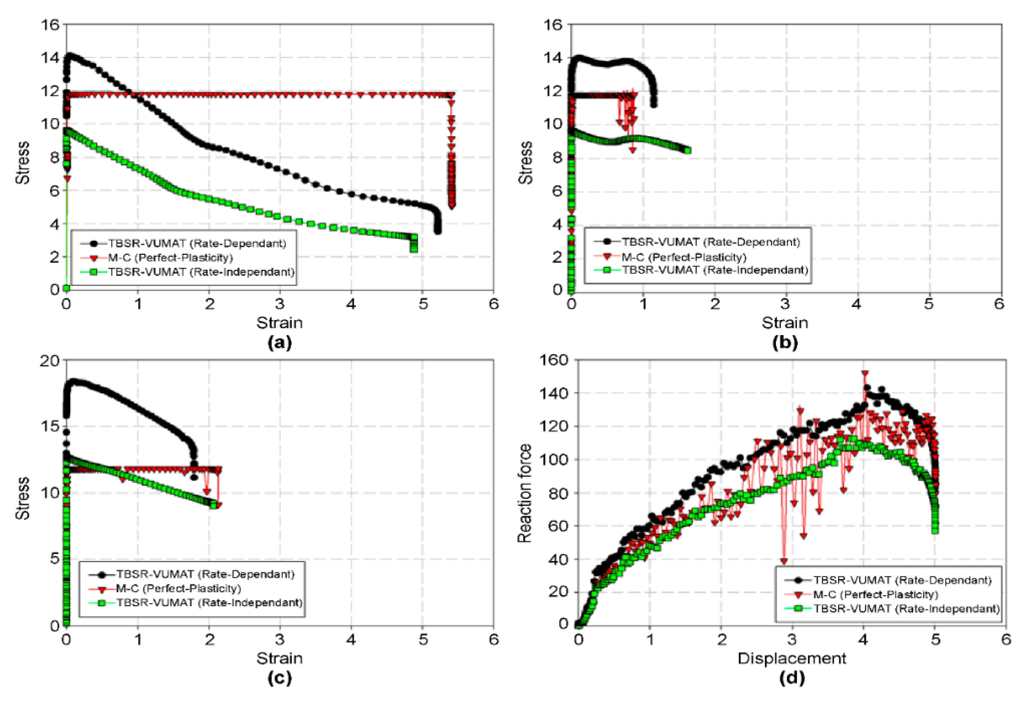
4.2. Results of the TBSR–VUMAT and M–C Models in the LDFE/CEL Model Analysis

To confirm the analysis results, as presented in Figure 11, the node point data were extracted. The results derived for Point 1 were set as the node immediately in front of the fluke of the anchor; Point 2 was set 5 m away from Point 1; and finally, Point 3 was assumed to be the location at which pipelines or cables were buried 5 m underground. Here, the behavior of the large-deformation soil was analyzed by deriving its stress–strain curve from the nodal results, and the reaction force–displacement curve results were obtained to examine the resistance of the soil according to the properties of each soil type. The results of the TBSR–VUMAT model were categorized into rate-dependent and rate-independent results and compared with those of the M–C model (Figure 12).

At Point 1 on the stress–strain curve of the soil, a large displacement occurs as the anchor drags and moves, causing a large strain. Furthermore, at Points 1 and 2, the results of the M–C model are located between the rate-dependent and rate-independent curves. All the models differ, and the M–C model generates stress in a straight line after yield.

However, in Figure 12c, the rate-independent curve displays a larger stress than the M–C model curve at Point 3, and the rate-dependent curve also exhibits higher stress than at Points 1 and 2. The soil begins to yield, and thereafter, the curve tends to decrease gradually owing to the softening effect. The change in the shear strength $S_u$, which varies depending on the depth of the ground set in the TBSR–VUMAT model, and the self-weight and upper part of the soil may be the underlying causes for this trend. As shown in Figure 12d, the rate dependence of the TBSR–VUMAT model produces the largest resistance in the ground. Furthermore, the resistance decreases in the order of M–C model > rate-independent TBSR–VUMAT. Compared with the result of composing the ground with the TBSR–VUMAT model, the result of the soil composed of the M–C model marginally deviated after yield, making it difficult to judge the accuracy of the result.

In particular, in the soil resistance trend, as the displacement increases, the results are not well expressed due to jaggedness. This characteristic was inferred to be due to poor analysis of the soil behavior after failure of the constructed soil. In addition, the FEA results obtained with tracer particles were analyzed to investigate the displacement of the ground for nodes in the depth direction (z-axis) from Points 1 and 2 in front of the anchor fluke (Figure 13). The results reveal different tracer particle behaviors between the models. In particular, the tracer particles set in the depth direction from Point 2 exhibit rather large differences among the three models. This tendency is due to the soil resistance from the front part. The displacement is the smallest in the rate-dependent case in which the resistance is the largest, and it is the largest in the rate-independent case. The same results were obtained for the depth of anchor penetration by dragging through all three types of ground. However, the behavior of the ground around the anchor is slightly different in each time zone.

5. Parametric Study

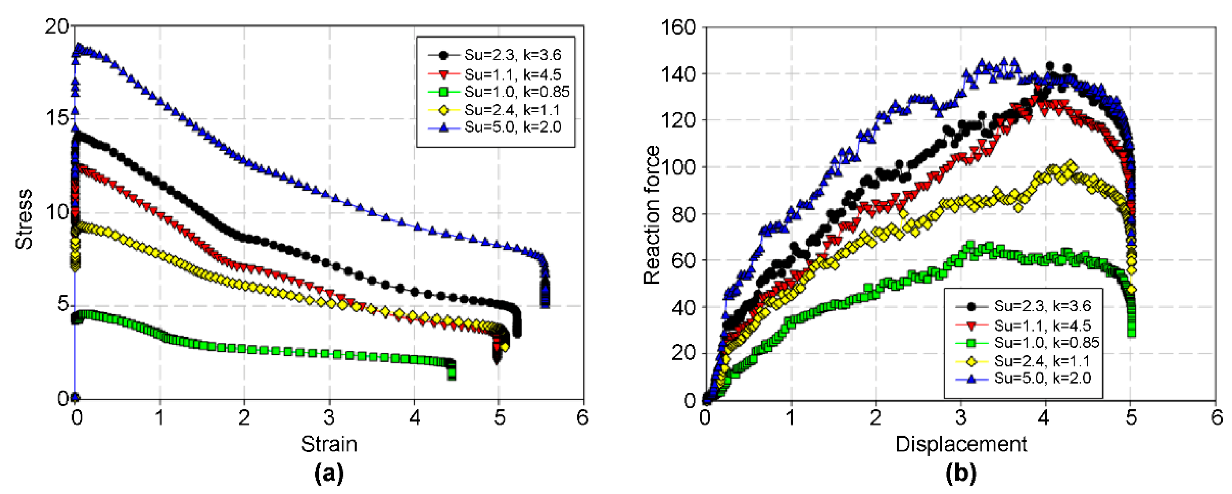
5.1. Soil Behavior According to the Effect of Undrained Shear Strength

The TBSR–VUMAT model expresses the shear strength to consider the strain-softening and strain-rate dependence of clay soil. This model was analyzed and compared with the commonly applied M–C model. However, there is a limit to the applicability of the fixed parameters among the various parameters related to the soil, as indicated in the shear strength formula in Equation (14). Therefore, it was necessary to verify the parameters in Equation (14).

First, to evaluate the effects of the undrained shear strength of the ground, an analysis was performed by referring to five cases with clay ground composed and verified by previous scholars [4,28,30,31]. The results for these five cases are illustrated in Figure 14.

Figure 14a depicts the stress–strain curve at Point 1 in each case, which indicates the compounded effects of the input values of $S_u{}_0$, $k$, and the difference in the yield stress. Similarly, in the force–displacement curve in Figure 14b, large differences are observed between the results obtained in the different cases; in particular, the largest value of 5 + 2 z [4] and the smallest value of 1.0 + 0.85 z [31] exhibit a three-fold difference. The value set according to the undrained shear strength and the depth of the ground had a large effect on the simulated ground. For accurate verification and comparison, the experimental results were obtained for the set parameters.

All results in Figure 14 were acquired considering strain-softening and strain-rate dependence. As described in the previous section, to investigate the effects of TBSR–VUMAT on the strain-softening and strain-rate dependence, four cases were explored: softening and rate dependence (S–D case); non-softening and rate dependence (NS–D case); softening and rate independence (S–ID case); and non-softening and rate independence (NS–ID case). Twelve sets of results, representing three results for each of the four cases above, are illustrated in Figure 15, with 5 + 2 z showing the largest results, 1.1 + 4.5 z showing the median results, and 1 + 0.85 z showing the smallest results.

Figure 15a–c present the stress–strain results, and Figure 15d–f depict the force–displacement results for the same cases as Figure 15a–c, respectively. First, the stress–strain results in Figure 15c reveal a large difference in the values depending on whether strain-softening and strain-rate dependence are considered. The gap narrows as the undrained shear strength decreases. In addition, in the case with a significantly small undrained shear strength (Figure 15b), the NS–ID and S–D cases show relatively similar stress results as the anchor is dragged. This is the result of the undrained shear strength of clay being sensitive to the strain rate when modeling the undrained shear strength of clay, and softening should be additionally considered for large deformation soil. The difference in the yield point and the softening effect in the early stage are not accurately simulated, and the difference increases toward the subsequent stage. The same tendencies are observed in Figure 15d–f. The results represented by the yellow square marks corresponding to the NS–ID case and the black circle marks corresponding to the S–D case are almost identical.

However, the results in the early and late stages are slightly different, confirming that it is essential to consider the effects of the strain softening and strain rate in the simulation of clay soil accompanied by large deformation.

5.2. Anchor Penetration Depth Results According to the Effects of Undrained Shear Strength

This section addresses the behavior and resistance of the soil. Moreover, in the anchor drag problem, it should be possible to determine the depth of penetration into the soil, i.e., whether the anchor is colliding with a submarine pipeline or cable under the seabed, which can be determined from the anchor penetration depth. The penetration depth in the soil according to the dragging distance of the anchor is presented in Figure 16. The trajectory of the anchor point penetrating the deepest end of the anchor fluke, i.e., the deepest point in the ground, was traced (Figure 15), and all three parameters of the undrained shear strength and the four results with or without consideration of strain-softening and strain-rate dependence were calculated. These results confirm shallow penetration due to anchor dragging, in the case in which the existing largest undrained shear strength of 5 + 2 z is applied. In addition, no significant difference exists between the results in the case of 1 + 0.85 z, corresponding to the smallest undrained shear strength, and 1.1 + 4.5 z, which is the median value. We inferred the presence of a limit to the anchor penetration depth for the effect of the undrained shear strength of the clay. In addition, in the previous force–displacement results, the S–D and NS–ID cases yielded similar results, as the increase in the strain rate was lost due to the softening effect. In the actual anchor drag results, all undrained shear strengths are distinct. This finding indicates that, considering the strain-softening and strain-rate dependence, different results are obtained when evaluating the risks to submarine pipelines and cables considering anchor dragging.

In addition, in all three undrained shear strength cases, the effect of the strain rate is large, and the anchor penetration is shallower than in the case in which it is not considered. Conversely, strain softening results in deeper anchor penetration than in the case in which it is not considered. The strain-softening and strain-rate dependence have rather large effects on the penetration depth when the anchor is dragging. However, it is necessary to verify the parameters reflecting the effects of strain-softening and strain-rate dependence, which requires a comparison of the present results with those of previous studies.

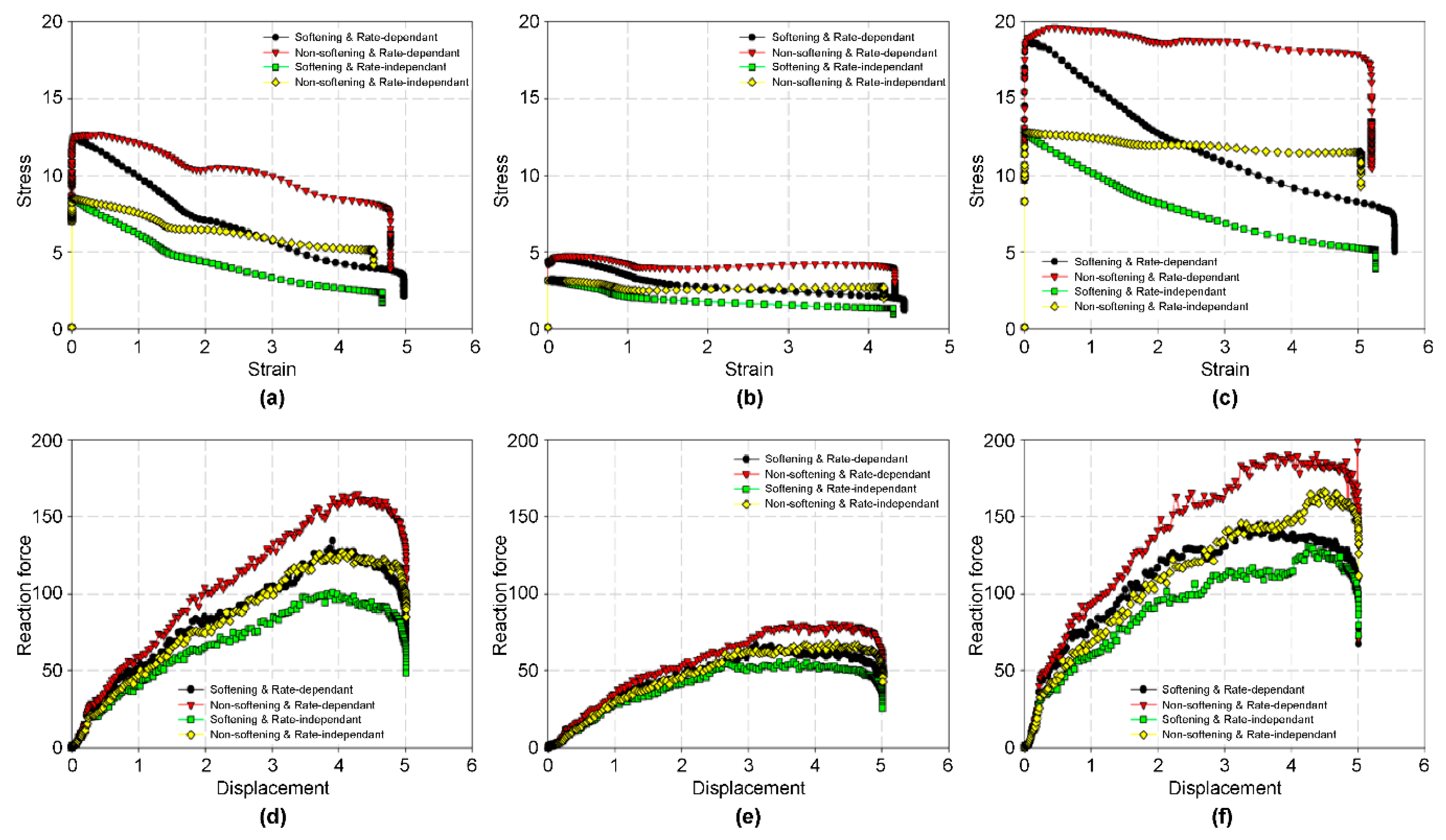
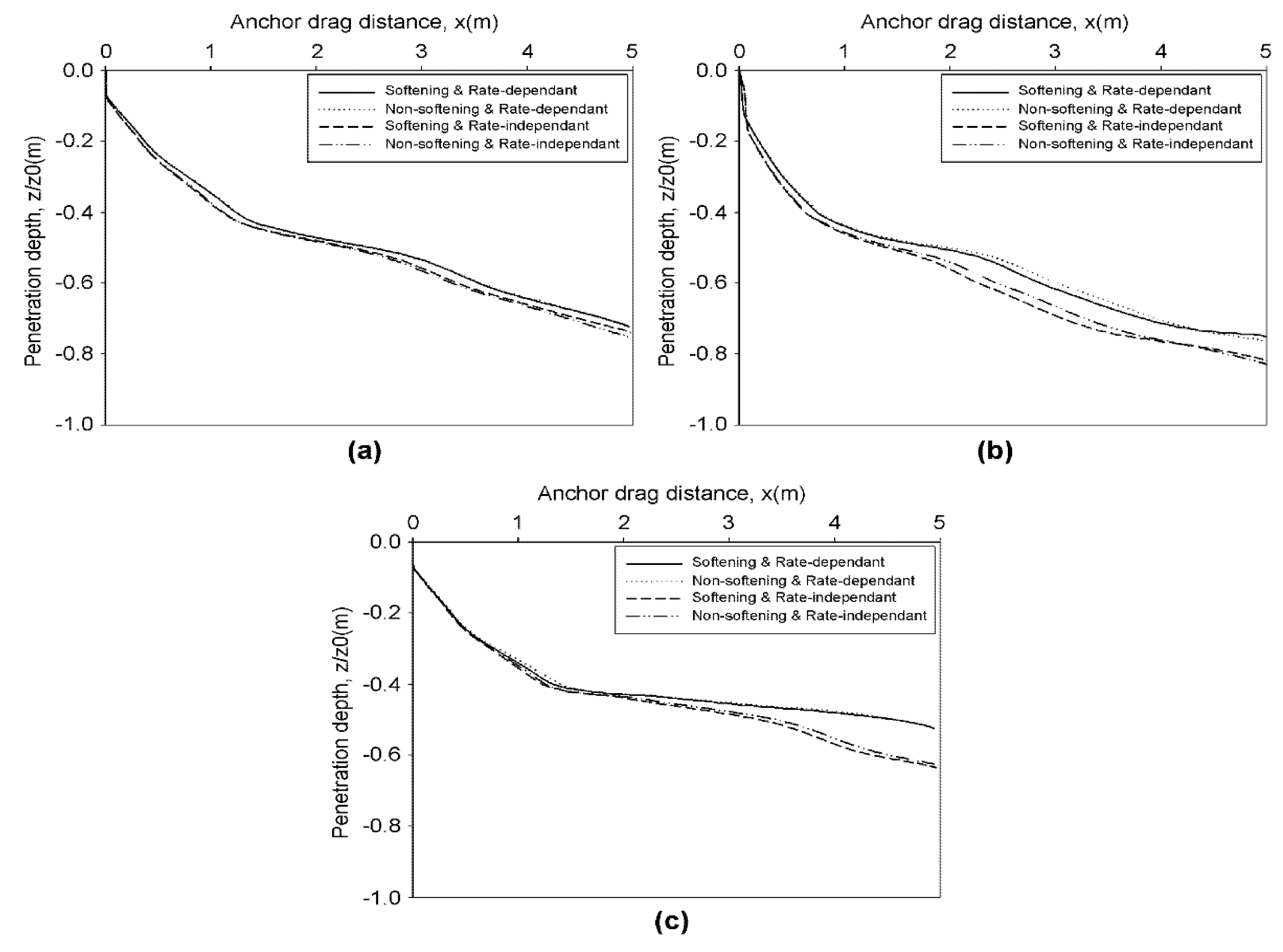
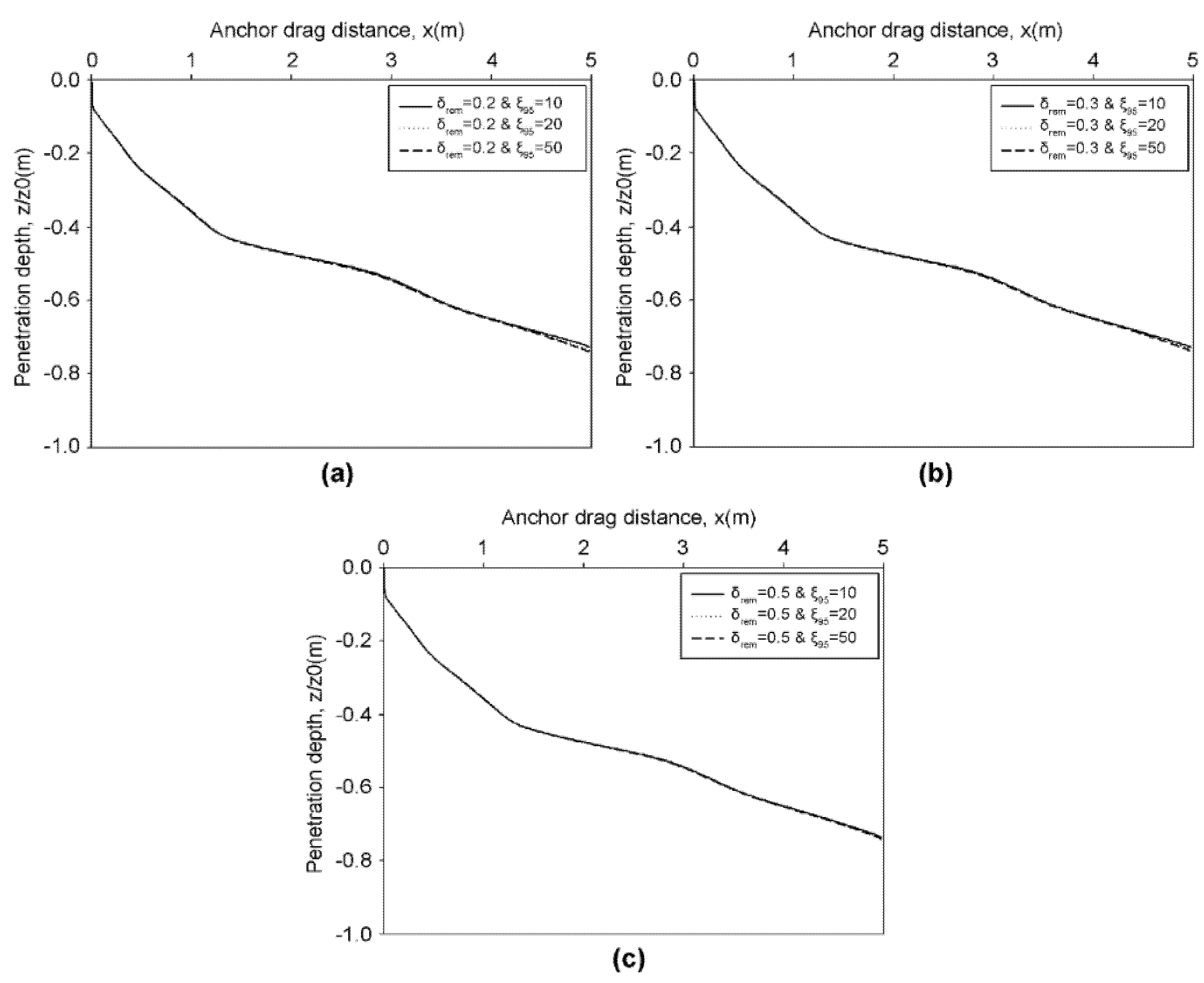
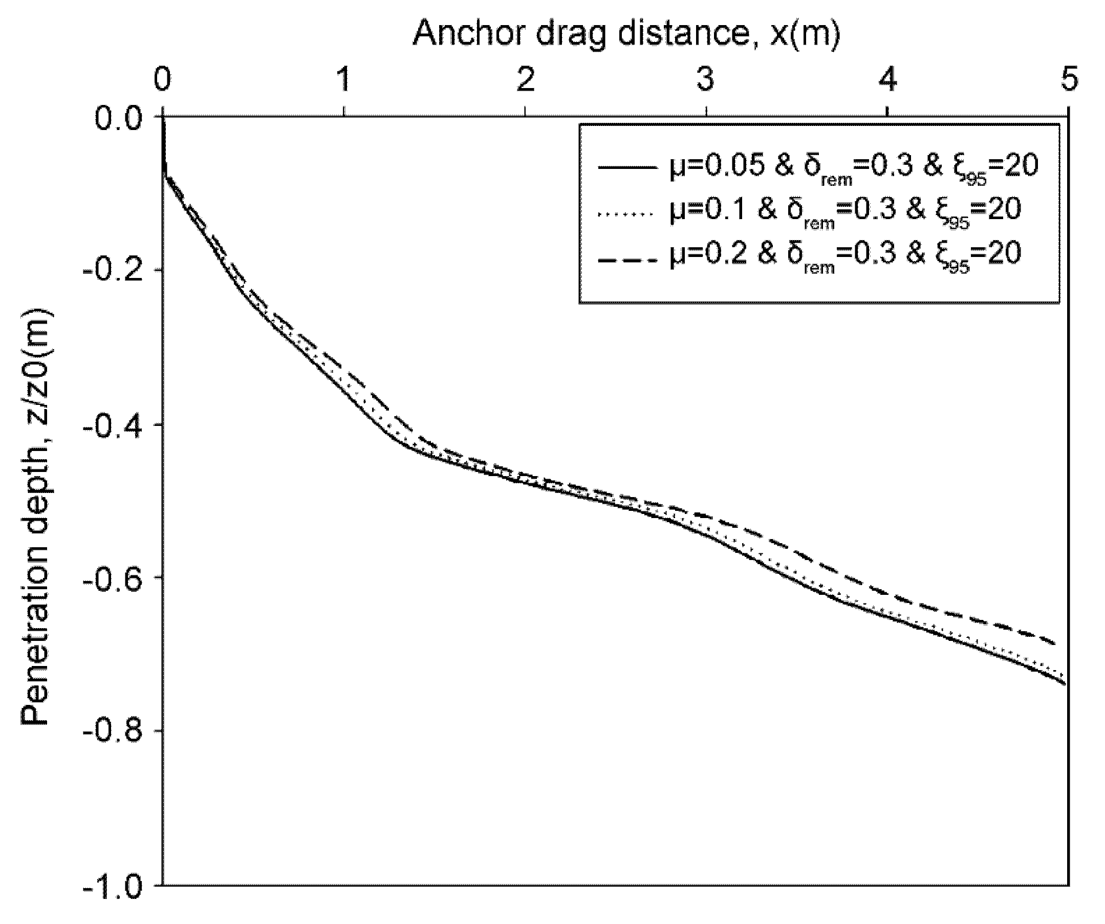
5.3. Anchor Penetration Depth According to the Effects of Strain-Softening and Strain-Rate Dependence

In this parametric study, the parameters listed in

Table 4. Strain-rate and strain-softening parameters.

Strain Rate	Strain Softening
Viscosity Parameter of Soil $\left(\mathsf{\mu }\right)$	Remolded Strenght Ratio of Soil $\left({\mathsf{\delta }}_{\mathit{r}\mathit{e}\mathit{m}}\right)$	Ductility Parameter of Soil $\left({\mathsf{\xi }}_{95}\right)$
0.05, 0.1, 0.2	0.2, 0.3, 0.5	10, 20, 50

were verified by applying the intermediate value 1.1 + 4.5 z, which was judged to limit the penetration depth compared with those in the undrained shear strength cases. The variables in Table 4 were sourced from Randolph [32]. Here, 27 cases were analyzed while changing the variables that determined the strain-softening effect based on $\mu$, which reflects the strain rate. The ground penetration depth of the anchor was calculated in each case. The results of the softening effect for a strain rate of 0.05 are illustrated in Figure 17. The differences between the results when ${\delta }_{rem}$ is fixed and ${\xi }_{95}$ is varied are insignificant. In particular, the error of the results for ${\xi }_{95}$ decreases as ${\delta }_{rem}$ increases. After the final dragging motion is completed, any differences in the final penetration depth disappear, and the results are nearly identical.

Figure 17a–c exhibit almost the same results, with no difference in the penetration depth. Note that the strain rate was fixed and the clay ground was simulated as proposed by Randolph (2004). The results are similar for all softening variables. Therefore, without analyzing additional cases, the effects of the strain rate with fixed softening parameters were derived from the results of the discussed cases (Figure 18). As shown in Figure 18, among the strain-softening parameters proposed by Randolph [32], the intermediate values of ${\delta }_{rem}$ = 0.3 and ${\xi }_{95}$ = 20 were implemented as default values, and the results were derived by varying $\mu$, a strain-rate variable.

The results are approximately identical to those obtained by varying the undrained shear strength in Figure 16. However, the results in Figure 17 are significantly different from those obtained by varying the strain-softening parameters. In addition, the strain-softening effect in the large-deformation soil is weak yet significant, and therefore, must be considered.

6. Conclusions

In this study, we improved large-deformation analysis and the TBSR-VUMAT model to simulate clay in which large deformation occurs and the effects of strain-softening and strain-rate dependence more accurately. We applied this analysis technique and model to the anchor drag phenomenon, and the results can be summarized as follows:

(1) The strain–stress and force–displacement curves of clay soil with anchor dragging were derived and compared with the results obtained using the existing M–C model for verification. The drag phenomenon was more clearly simulated in the clay soil accompanied by large deformation in the newly developed model than in the M–C model. An numerical analysis confirmed the theoretical effects of strain-softening and strain-rate dependence.

(2) To verify the soil parameters in the anchor-drag problem, they were analyzed by varying the undrained shear strength. Five distinct types of undrained shear strength were applied. The effects of strain-softening and strain-rate dependence were also simulated. As part of the analysis, the force–displacement curve confirmed that the ratio increased by the strain rate effect was decreased to a certain extent by the softening effect, showing similar results among all cases analyzed. However, the anchor penetration depth analysis, which is fundamental to the anchor-drag problem, confirmed that the results were clearly different between the cases in which these two effects were considered.

(3) A parametric study of the strain-softening and strain-rate dependence clarified the effect of the strain rate, as well as the weak effect of strain softening. In large-deformation soil, such as that deformed due to anchor drag, it is essential to consider the effects of strain-softening and strain-rate dependence. In particular, the basic analysis to be performed when setting the variables in clay soil was conducted in this study, and the results were compared and analyzed.

This study demonstrates that the TBSR–VUMAT model can be improved as the M–C model base, and thereby, extended to silt or sandy soil, in addition to clay soil.

References

1. Kim, Y.H.; Jeong, S.S. Analysis of Dynamically Penetrating Anchor Based on Coupled Eulerian-Lagrangian (CEL) Method. J. Korean Soc. Civ. Eng. 2014, 34, 895–906. [Google Scholar] [CrossRef] [Green Version]
2. Han, C.C.; Chen, X.J.; Liu, J. Physical and Numerical Modeling of Dynamic Penetration of Ship Anchor in Clay. J. Waterw. Port Coast. Ocean Eng. 2019, 145, 04018030. [Google Scholar] [CrossRef]
3. Shin, M.B.; Park, D.S.; Seo, Y.K. Design of Rock-Berm by Anchor Dragging Simulation Using CEL Method. J. Ocean Eng. Technol. 2017, 31, 397–404. [Google Scholar] [CrossRef] [Green Version]
4. Hossain, M.S.; Kim, Y.H.; Gaudin, C. Experimental Investigation of Installation and Pull-Out of Dynamically Penetrating Anchors in Clay and Silt. J. Geotech. Geoenviron. Eng. 2014, 140, 04014026. [Google Scholar] [CrossRef] [Green Version]
5. Kim, Y.H.; Hossain, M.S. Dynamic Installation of OMNI-Max Anchors in Clay: Numerical Analysis. Géotechnique 2015, 65, 1029–1037. [Google Scholar] [CrossRef] [Green Version]
6. Liu, H.X.; Xu, K.; Zhao, Y.B. Numerical Investigation on the Penetration of Gravity Installed Anchors by a Coupled Eulerian-Lagrangian Approach. Appl. Ocean Res. 2016, 60, 94–108. [Google Scholar] [CrossRef]
7. Hamann, T.B.; Qiu, G.; Grabe, J.G. Application of a Coupled Eulerian-Lagrangian Approach on Pile Installation Problems Under Partially Drained Conditions. Comput. Geotech. 2015, 63, 279–290. [Google Scholar] [CrossRef]
8. Bhattacharya, P. Pullout Capacity of Strip Plate Anchor in Cohesive Sloping Ground Under Undrained Condition. Comput. Geotech. 2016, 78, 134–143. [Google Scholar] [CrossRef]
9. Merifield, R.S.; Lyamin, A.V.; Sloan, S.W. Stability of Inclined Strip Anchors in Purely Cohesive Soil. J. Geotech. Geoenviron. Eng. 2005, 131, 792–799. [Google Scholar] [CrossRef]
10. Song, Z.; Hu, Y.; Randolph, M.F. Numerical Simulation of Vertical Pullout of Plate Anchors in Clay. J. Geotech. Geoenviron. Eng. 2008, 134, 866–875. [Google Scholar] [CrossRef]
11. Wang, D.; Hu, Y.; Randolph, M.F. Three-Dimensional Large Deformation Finite-Element Analysis of Plate Anchors in Uniform Clay. J. Geotech. Geoenviron. Eng. 2010, 136, 355–365. [Google Scholar] [CrossRef]
12. Wang, Q.; Zhou, X.W.; Zhou, M.; Hu, Y.X. Inner Soil Heave of Stiffened Caisson During Installation in Soft-Over-Stiff Clay. Comput. Geotech. 2021, 138, 104336. [Google Scholar] [CrossRef]
13. Ma, H.; Zhou, M.; Hu, Y.; Shazzad Hossain, M. Interpretation of Layer Boundaries and Shear Strengths for Soft-Stiff-Soft Clays Using CPT Data: LDFE Analyses. J. Geotech. Geoenviron. Eng. 2016, 142, 04015055. [Google Scholar] [CrossRef] [Green Version]
14. Huang, Z.; Yin, F.; Li, Z.; Liu, Y.B. Numerical Simulation of Drag Anchor Trajectory in Non-linear Soil Based on CEL Method. In Proceedings of the 31st International Ocean and Polar Engineering Conference, Rhodes, Greece, 20–25 June 2021; pp. 1339–1345. [Google Scholar]
15. Liu, H.X.; Liang, K.; Peng, J.S.; Xiao, Z. A Unified Explicit Formula for Calculating the Maximum Embedment Loss of Deepwater Anchors in Clay. Ocean Eng. 2021, 236, 109454. [Google Scholar] [CrossRef]
16. Cassidy, M.J. Experimental Observations of the Penetration of Spudcan Footings in Silt. Géotechnique 2012, 62, 727–732. [Google Scholar] [CrossRef]
17. Clausen, J.; Damkilde, L.; Andersen, L. Efficient Return Algorithms for Associated Plasticity With Multiple Yield Planes. Int. J. Numer. Methods Eng. 2006, 66, 1036–1059. [Google Scholar] [CrossRef]
18. ABAQUS. ABAQUS User’s Manual; Dssault Systems; ABAQUS: Paris, France, 2018. [Google Scholar]
19. Einav, I.; Randolph, M.F. Combining Upper Bound and Strain Path Methods for Evaluating Penetration Resistance. Int. J. Numer. Methods Eng. 2005, 63, 1991–2016. [Google Scholar] [CrossRef]
20. Zhou, H.; Randolph, M.F. Computational Techniques and Shear Band Development for Cylindrical and Spherical Penetrometers in Strain-Softening Clay. Int. J. Geomech. 2007, 7, 287–295. [Google Scholar] [CrossRef]
21. Wilkins, M. Calculation of Elastoplastic Flows. Methods Comp. Physiol. 1964, 3, 211–263. [Google Scholar]
22. Maenchen, G.; Sack, S. The Tensor Code. Methods Comp. Physiol. 1964, 3, 12–35. [Google Scholar]
23. Kong, D. Large Displacement Numerical Analysis of Offshore Pipe-Soil Interaction on Clay. Ph.D. Thesis, University of Oxford, Oxford, UK, 2015. [Google Scholar]
24. Hazell, E. Numerical and Experimental Studies of Shallow Con Penetration in Clay. Ph.D. Thesis, University of Oxford, Oxford, UK, 2008. [Google Scholar]
25. Hill, R.; Lee, E.H.; Tupper, S.J. The Theory of Wedge Indentation of Ductile Materials. Proc. R. Soc. Lond. A Math. Phys. Eng. Sci. 1945, 188, 273–290. [Google Scholar]
26. Hossain, M.S.; Randolph, M.F. Effect of Strain Rate and Strain Softening on the Penetration Resistance of Spudcan Foundations on Clay. Int. J. Geomech. 2009, 9, 122–132. [Google Scholar] [CrossRef]
27. Das, B.M. Principles of Geotechnical Engineering, 7th ed.; Cengage Learning: Sacramento, CA, USA, 2002. [Google Scholar]
28. Dingle, H.R.C.; White, D.J.; Gaudin, C. Mechanisms of Pipe Embedment and Lateral Breakout on Soft Clay. Can. Geotech. J. 2008, 45, 636–652. [Google Scholar] [CrossRef]
29. Ryu, D.M.; Lee, C.S.; Choi, K.H.; Koo, B.Y.; Song, J.K.; Kim, M.H.; Lee, J.M. Lab-Scale Impact Test to Investigate the Pipe-Soil Interaction and Comparative Study to Evaluate Structural Responses. Int. J. Nav. Arch. Ocean Eng. 2015, 7, 720–738. [Google Scholar] [CrossRef]
30. Lee, Y.S. Physical and Numerical Modelling of Pipe-Soil Interaction in Clay. Ph.D. Thesis, The University of Sheffield, Sheffield, UK, 2012. [Google Scholar]
31. Zimmerman, E.H.; Smith, M.W.; Shelton, J.T. Efficient Gravity Installed Anchor for Deep Water Mooring. In Proceedings of the Offshore Technology Conference, Houston, TX, USA, 4 May 2009. paper OTC20117. [Google Scholar]
32. Randolph, M.F. Characterization of Soft Sediments for Offshore Applications. In Proceedings of the 2nd International Conference on Site Characterization, Porto, Portugal, 1 January 2004; pp. 209–231. [Google Scholar]
Figure 1. Eulerian volume fraction.
Jmse 10 01734 g001
Figure 2. Linear yield criteria in principal stress space [17]. (a)Tresca model; (b)M–C model.
Jmse 10 01734 g002
Figure 3. Principle of return mapping [17].
Jmse 10 01734 g003
Figure 4. Plane surfaces from the Tresca yield surface [23].
Jmse 10 01734 g004
Figure 5. Verification results.
Jmse 10 01734 g005
Figure 6. Indentation mechanism of a smooth wedge.
Jmse 10 01734 g006
Figure 7. Coupled Eulerian–Lagrangian (CEL) model illustrating the mesh topography.
Jmse 10 01734 g007
Figure 8. Influence of β on wedge indentation in CEL analysis [25].
Jmse 10 01734 g008
Figure 9. Dimensions of the stow net anchor (AGM anchor).
Jmse 10 01734 g009
Figure 10. Large deformation finite element (LDFE) modeling using the CEL method.
Jmse 10 01734 g010
Figure 11. Points used for the observation and analysis of the results.
Jmse 10 01734 g011
Figure 12. Results of TBSR–VUMAT and M–C models. (a) Point 1, (b) Point 2, (c) Point 3, and (d) force–displacement curve.
Jmse 10 01734 g012
Figure 13. Results of TBSR–VUMAT and M–C models. (a) M–C model, (b) TBSR–VUMAT model in the rate-dependent case, and (c) TBSR–VUMAT model in the rate-independent case.
Jmse 10 01734 g013
Figure 14. Results of the TBSR–VUMAT model according to undrained shear strength. (a) Stress–strain curve and (b) force–displacement curve.
Jmse 10 01734 g014
Figure 15. Results of TBSR–VUMAT model according to strain softening and strain rate (a,d) 1.1 + 4.5 z, (b,e) 1.0 + 0.85z, and (c,f) 5 + 2 z.
Jmse 10 01734 g015
Figure 16. Anchor penetration depths obtained from TBSR–VUMAT model according to strain softening and rate: (a) 1.1 + 4.5 z, (b) 1+ 0.85 z, and (c) 5 + 2 z.
Jmse 10 01734 g016
Figure 17. Anchor penetration depths of the TBSR–VUMAT model for a strain rate of 0.05 when δ r e m is (a) 0.2, (b) 0.3, and (c) 0.5.
Jmse 10 01734 g017
Figure 18. Effects of strain rate on anchor penetration depth.
Jmse 10 01734 g018