
Normalized Radar Scattering Section Simulation and Numerical Calculation of Freak Wave


College of Computer Science and Engineering, Shandong University of Science and Technology, Qingdao 266590, China
*
Author to whom correspondence should be addressed.
J. Mar. Sci. Eng. 2022, 10(11), 1631; https://doi.org/10.3390/jmse10111631
Submission received: 26 September 2022
/
Revised: 23 October 2022
/
Accepted: 27 October 2022
/
Published: 2 November 2022
(This article belongs to the Special Issue Extreme Coastal and Ocean Waves)
Abstract
:The improved phase modulation method is used to numerically simulate a two-dimensional freak wave. While generating freak waves at specific positions, the spectral structure of the target spectrum can also be maintained, and the statistical characteristics of wave sequences can be satisfied. The numerical simulation process is discussed in detail from the perspective of different wave spectra and other parameters, the priority applicability of the Joint North Sea Wave Project (JONSAWP) spectrum is determined, and the accuracy of the numerical simulation is significantly improved. At the same time, the electromagnetic scattering characteristics of freak waves are studied based on the two-scale method (TSM). The calculation results of normalized radar cross section (NRCS) under different wave spectra and different polarization modes are compared, and the effects of wind speed, incident frequency, and incident angle on the calculation results are discussed. Experiments show that the NRCS of the freak wave is obviously lower than the background wave, and the calculation of the NRCS is relatively simple. This provides an effective reference for radar detection of freak waves in offshore engineering.
1. Introduction
A freak wave is an extreme wave with a prominent wave crest, concentrated energy, and strong destructive power. The concept of a freak wave was first proposed by Draper [1]. Its wave height is generally greater than or equal to twice the wave height of the background wave. According to marine observation records, freak waves appear in all major sea areas in the world, and there are few actual measurement records. Didenkulova et al. [2] documented accidents of freak waves and the damage they caused during 2019–2021. Even if the return period of extreme waves is very long, they are usually not considered in the design of offshore structures [3]. Since the appearance of a freak wave is sudden and unpredictable, it will cause serious harm to marine structures and ship safety [4,5,6]. Based on this, freak waves have attracted more and more researchers’ attention. Wang et al. [7] used computational fluid dynamics to numerically simulate the well-known freak wave “New Year Wave”. Gao et al. [8], using the fully nonlinear Boussinesq model, FUNWAVE 2.0, simulated the focused transient wave group and studied its interactions with the harbor. Fedele et al. [9] used the WAVEWATCH III wave model and Higher Order Spectral method (HOS) to study the physical and statistical characteristics of freak waves by comparing the measured records of freak waves. Amrutha et al. [10] recorded the wave statistical parameters during Cyclone Phailin’s passage through the northern Bay of Bengal in October 2013, during which eight freak wave events were observed. They recorded the relevant wave heights and kurtosis, which provided an important reference for the study of freak waves. Zhang [11] used the Peregrine breathing solution model to simulate the freak wave and established a three-dimensional hull structure model. Zeng et al. [12] proposed inserting an extreme wave into the carrier sequence in the time domain to generate a freak wave; it can conveniently modulate the freak wave profile while maintaining the waveform at other moments. At present, there are also some advances in the research on the prediction of freak waves. Doong et al. [13] used the artificial neural network model to predict the probability of coastal freak waves. Cui et al. [14] established the linear regression relationship between the spatial position of the largest wave crest and instantaneous moment and proposed a method to predict the freak wave speed through regression analysis and studied the nonlinear characteristics of the freak wave speed. In addition, many researchers have studied the formation of freak waves and their effects on offshore structures [15,16,17,18].
In practical engineering, we can combine electromagnetic scattering technology with the ocean to study some characteristics of the ocean or identify the characteristics of the ocean. For example, Mansoori et al. [19] used the SPM small perturbation scattering method to simulate the NRCS of clean and oil-polluted sea ice to distinguish clean and oil-polluted sea ice. Wei et al. [20] used an NRCS calculation method based on the ratio of median and mean to improve the wind speed retrieval of high-resolution SAR under pollution conditions. Schulz-Stellenfleth et al. [21] analyzed synthetic aperture radar (SAR) images from Environmental Research Satellites and proposed a method to retrieve sea wave parameters from SAR, which can realize a reasonable estimation of significant wave height. The research of Hopkin [22] and Van Groesen et al. [23,24] provides a reference for the observation and prediction of freak waves using radar snapshots. In addition, some researchers propose to predict the sea surface through radar images [25,26]. In recent years, many studies have proved the feasibility of applying radar and electromagnetic scattering technology to monitor and identify the sea surface. The research on the prediction of freak waves mainly focuses on wave height, the interaction between waves, the sea state, water depth, and other factors. However, there are relatively few studies on the use of electromagnetic scattering models to calculate and analyze simulated freak waves, study the related characteristics of freak waves, and identify freak waves. In this paper, an improved phase modulation method is used to numerically simulate a two-dimensional freak wave. Based on the Longuet-Higgins random wave theory, by adjusting the initial phases of some of the constituent waves to keep some wave surfaces always positive, the freak wave can be generated at specific locations. In order to improve the accuracy and efficiency of the numerical simulation of freak waves, we have discussed the simulation process in detail for different wave spectra, the different number of constituent waves, and the different modulation ratios, and we reference wave steepness. This effectively improves the accuracy of our numerical simulations. The study of theoretical calculation of electromagnetic scattering from stochastic rough sea surfaces has always been a very important research topic. On the basis of the numerical simulation results, we combined the electromagnetic scattering theory to calculate the backscattering coefficient of the freak wave and compared and studied the scattering characteristics of the freak wave. Moreover, we discuss the effects of different wind speeds, different incident frequencies, and different incident angles on the experimental results.
2. Wave Spectra Model and Numerical Simulation Model
2.1. Wave Spectrum Model
2.1.1. JONSWAP Spectrum
The JONSWAP spectrum [27] is derived from a large number of field measurements and statistical analyses outside the border coastlines of Germany and Denmark by several countries. The JONSWAP spectrum is considered to be the international standard ocean wave spectrum. The JONSWAP spectrum indicates that the wind and waves are in a growing state, and the peak value of the spectrum is higher. Moreover, the JONSWAP spectrum can be transformed into the JONSWAP TMA spectrum for arbitrary water depth [28,29]. Its expression is:
where is the dimensionless constant, is the peak elevation factor, is the peak shape parameter, is the peak frequency when , , when , , and is the acceleration of gravity. The JONSWAP spectrum can be transformed into the P-M spectrum for .
2.1.2. Wen’s Spectrum
Wen’s spectrum summarizes and analyzes the existing wave spectrum models through analytical methods. It describes the different stages of wind and wave growth and applies them to different water depths. After deduction and improvement, the simplified expression of “Wen’s Improved Spectrum” [30] was obtained:
where , , , , , and represent the significant wave height and significant period, respectively.
2.1.3. PM Spectrum
The PM spectrum is the result of Pierson and Moskowitz [31] through the analysis and statistics of fully developed wave data in the North Atlantic Ocean in 1964. It is an empirical spectrum suitable for fully developed seas. Its expression is:
where , is the wind speed at 19.5m from the sea surface, and is the acceleration of gravity.
2.2. Numerical Simulation Method of Freak Wave
In Longuet-Higgins‘s random wave theory [32], countless cosine waves with different periods, wave heights, and initial phases are linearly superimposed to represent the wave surface equation at a fixed position at any time. The basic expression is:
where is the instantaneous height of the wave surface of the i-th constituent wave relative to the still water surface, represents the number of constituent waves, are the initial phase, amplitude, angular frequency and the number of waves of the i-th constituent wave. The wave surface is obtained by combining the amplitude with the wave spectrum. Based on focusing the energy of random waves to simulate freak waves, we adjust the initial phases of some of the constituent waves to keep the statistical characteristics of the simulated random waves consistent with those of natural ocean waves [33]. First, we assume that a freak wave occurs at time and position , and we adjust the initial random phase to make take a positive value. The constituent wave is divided into two superimposed waves and , and the above expression is rewritten as the superimposed wave surface of the freak wave and the background wave:
Assuming that the constituent wave is focused on a specific position to produce a freak wave, we need to modulate this part of the random phase to make , we need to discuss the range of :
When , we set the integer , that is, the round-down operation for . We can know that , then is a positive value slightly smaller than , , at this time, we want to make , that is, , . When , since includes four quadrants, we discuss it in four cases:
When ,;
When ,;
When ,
;
When ,.
When , the discussion method is the same as above, and the range of can also be obtained. At this time, the waveform formed by the superposition of and will have waves as positive amplitude waves so that is a positive value, thus forming a freak wave.
2.3. Calculation Model of Electromagnetic Scattering of Freak Wave
Since the actual rough sea surface is irregular, we use the two-scale method (TSM) [34] combining the small perturbation method (SPM) [35] of the small rough surface and the Kirchhoff approximation (KA) [36] method of the large rough surface when calculating the electromagnetic scattering of the rough sea surface. The scattering coefficient is numerically equal to four times the ratio of the total scattered power to the total incident power, and its expression is:
where is generally the distance between the source of the scattered wave and the scattering target (such as freak wave surface), is the scattering power in this direction, is the incident field and represents the irradiation area. Based on the theory of TSM, the calculation method [37] of the backscattering coefficient is:
The two-scale method divides the rough surface into large-scale waves and small-scale waves. Large-scale wave is the gravity wave fluctuation of a rough wave, while the small-scale wave is the micro rough fluctuation on a large-scale wave. Moreover, represents the ensemble average operation for small-scale waves based on the surface slope of large-scale waves. We know that the components of water waves that resonate with electromagnetic waves are called Bragg waves. The relation between Bragg wavelength and incident electromagnetic wave wavelength is:
represents the incident angle of the electromagnetic wave. When the incident wavelength is determined, the number of waves satisfying belongs to the small rough size part in the TSM method ( is the incident wavenumbers and is the small rough size cutoff wavenumbers), we use the SPM method to calculate the scattered field. in Equation (9) can be expressed as:
where and represent the backscattering coefficients calculated in the vertical and horizontal polarization modes, respectively, and represent the backscattered fields of small-scale surface roughness under the vertical and horizontal polarization modes. and represent the incident angles in the global coordinate system and local coordinate system, respectively. , , , represent the vertical and horizontal polarization vectors in global and local coordinates, respectively. Combined with the definition of the scattering coefficient in Equation (8), the backscattering coefficient of the SPM method is:
where represents the incident wave number, represents the relative permittivity of seawater, and represents the two-dimensional ocean wave spectrum. The number of waves satisfying belongs to the large rough size part of the TSM method ( is the small rough size cutoff wavenumbers). We use the KA method to calculate the scattered field, and its backscattering coefficient is:
where is the probability density function of the surface slope. , , , , , where , , , and represent incident angle, scattering angle, incident azimuth angle, and scattering azimuth angle, respectively, and represents the imaginary unit. is the polarization coefficient. Scattering calculation is performed by Fresnel reflection coefficients , , where , .
3. Results and Discussion
3.1. Simulation and Analysis of Freak Wavel
In this paper, three classic ocean wave spectra, including the JONSWAP spectrum, PM spectrum, and Wen’s spectrum, are selected as the target spectrum for comparative analysis. According to the definition of freak wave [38], are the characteristic parameters of the freak wave, where , , , , represents the significant height of the background wave, represents the height of the freak wave, , respectively represent the wave heights of the two waves immediately before and after the freak wave in the simulation sequence and is the crest height of the freak wave.
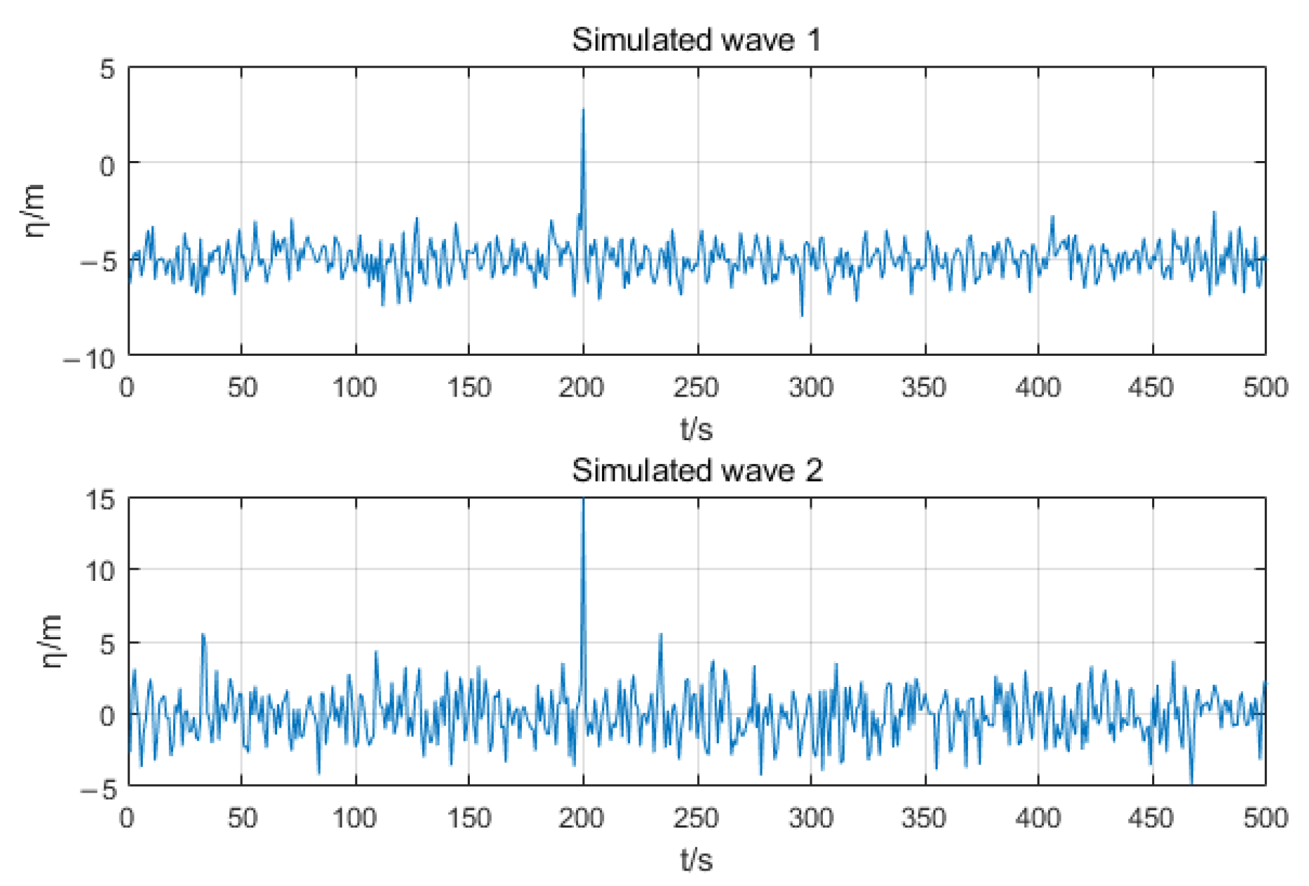
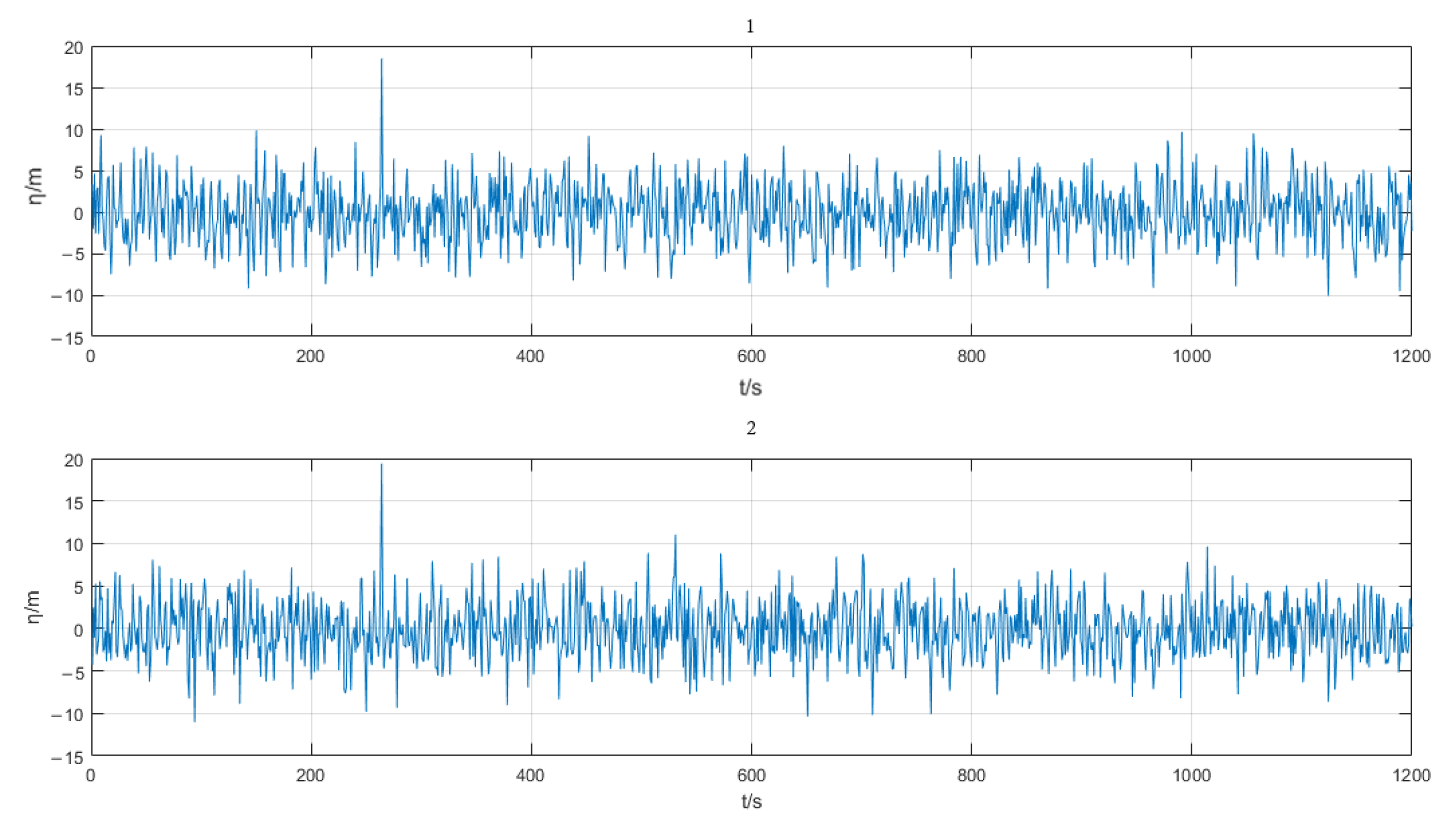
The experiment first uses the JONSWAP spectrum as an example, selects the spectral rise factor , the water depth , the peak period of the spectrum is , the number of constituent waves is selected as 200, the significant wave height , the number of modulated waves is selected as 160. Figure 1 shows the two simulation results of the time series of freak waves.
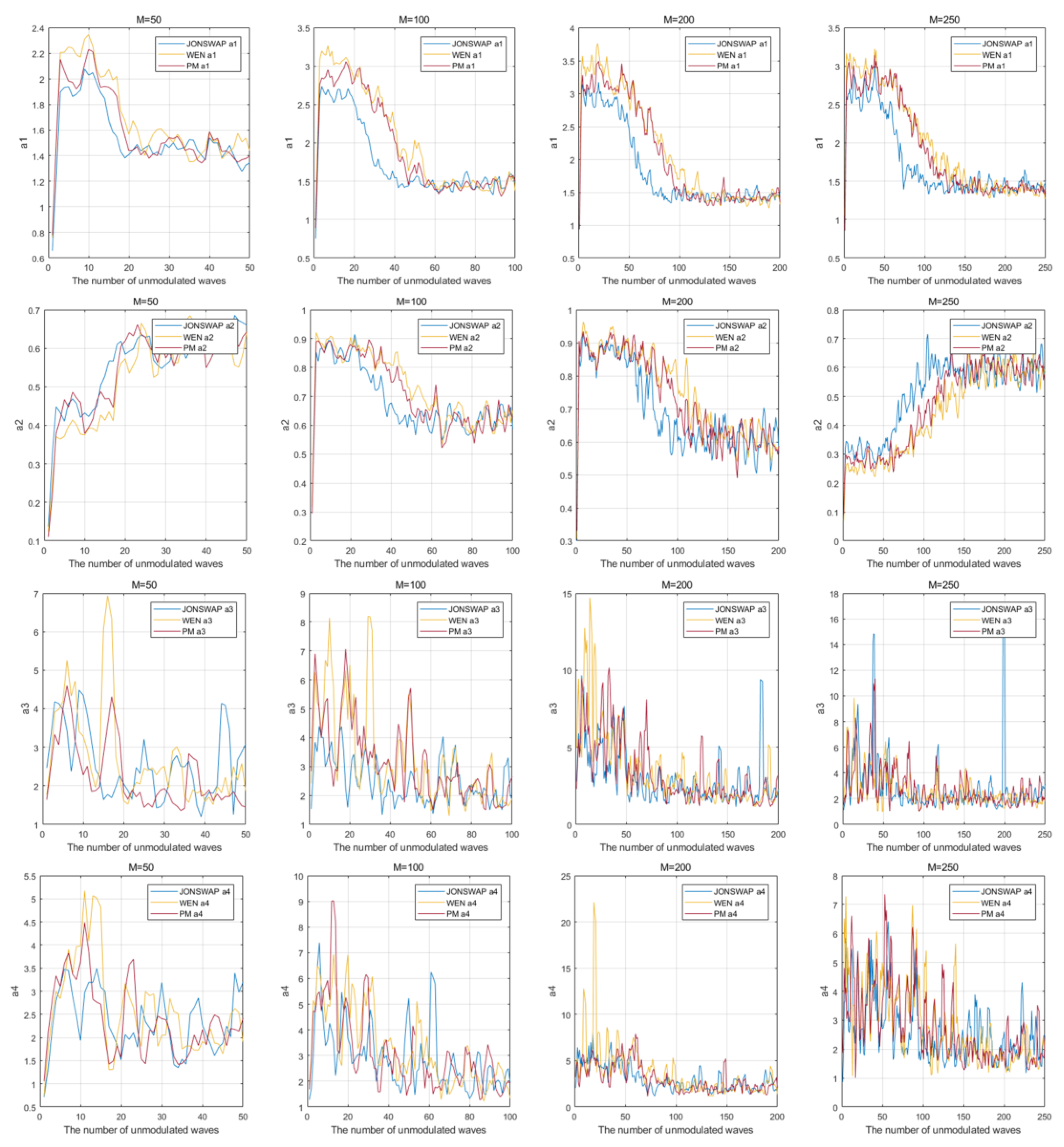
In the above experiment, the selection of the number of modulated waves is a theoretical empirical value. In Figure 1, the simulated wave 1 is a freak wave that meets the definition, but the simulated wave 2 is not a freak wave (a4 = 1.12). After many experiments, under this modulation ratio, there is also a situation where the generation of freak waves cannot be simulated. Therefore, we discuss the numerical calculation of a more accurate and efficient two-dimensional freak wave by selecting a different number of constituent waves and setting specific modulation ratios under a given number of constituent waves and comparing the differences between different wave spectra. We take the number of constituent waves of 50, 100, 200, and 250 as examples for comparison and verification. In order to ensure the accuracy of the experimental results, we use the number of unmodulated waves within the range of all numbers of constituent waves to correspond to the values of the basic indicators a1, a2, a3, and a4 of the freak wave and the comparison results are shown in Figure 2.
It can be seen that a1 and a2 can more intuitively see the range that meets the definition. Record the qualified a1 and a2 of each wave spectra in the experiment under different numbers of constituent waves in Table 1:
It can be seen from Table 1 that when the number of constituent waves is 100 and 200, the proportion of a1 and a2 that conform to the basic indicators of a freak wave is the highest. When the number of constituent waves is 100, the proportion of the basic index of a freak wave is similar to that when the number of constituent waves is 200, but the latter is slightly higher. Combined with the above results, we choose the number of constituent waves of 200 for the next experiment. Since not all freak waves can be generated when the number of constituent waves is 200, we will continue to discuss the selection of modulation interval. After many experiments, we can obtain the preliminary modulation range of three wave spectra through a1 and a2: the number of modulated waves of the JONSWAP spectrum is 141–200, the number of modulated waves of Wen’s spectrum is 111–200, and the number of modulated waves of PM spectrum is 121–200. It can be seen from Figure 2 that the three wave spectra fluctuate greatly within the conditions of a3 and a4, and the specific range cannot be determined intuitively. Therefore, we choose to conduct experiments on the three wave spectra within the range satisfying a1 and a2 and judge the optimal modulation interval by the number of freak waves generated in each interval. In order to eliminate the uncertain influence of the random initial phase of the constituent wave on the simulation results as much as possible, we conducted 1000 same experiments and selected 150 typical ones, and recorded the interval numbers that satisfying the conditions of a3 and a4 in Table 2, respectively. We do not record those that are not within each wave spectrum interval.
It can be seen from Table 2 that under the premise that the number of constituent waves is 200, the number of freak waves generated by JONSWAP spectrum simulation is the largest within the number of modulated waves of 171–180, while the number of freak waves generated by the number of modulated waves within the range of 141–150 is the least, which is only 899. The number of freak waves generated by Wen’s spectrum simulation is the largest within the number of modulated waves of 171–180, while the number of freak waves generated by the number of modulated waves within the range of 111–120 is the least, which is only 957. The number of freak waves generated by PM spectrum simulation is the largest within the number of modulated waves of 151–160, while the number of freak waves generated by the number of modulated waves within the range of 121–130 is the least, which is only 990. Analysis of the above experimental results shows that under the premise that the number of constituent waves is 200, with the increase of the number of modulated waves, the number of freak waves generated by the three wave spectra simulations shows a roughly increasing trend. Moreover, the total number of simulated freak waves generated by the three wave spectra is the largest when the number of modulated waves is within 171–180, which is the smallest difference from the number of simulated freak waves when the number of modulated waves is within 151–160.
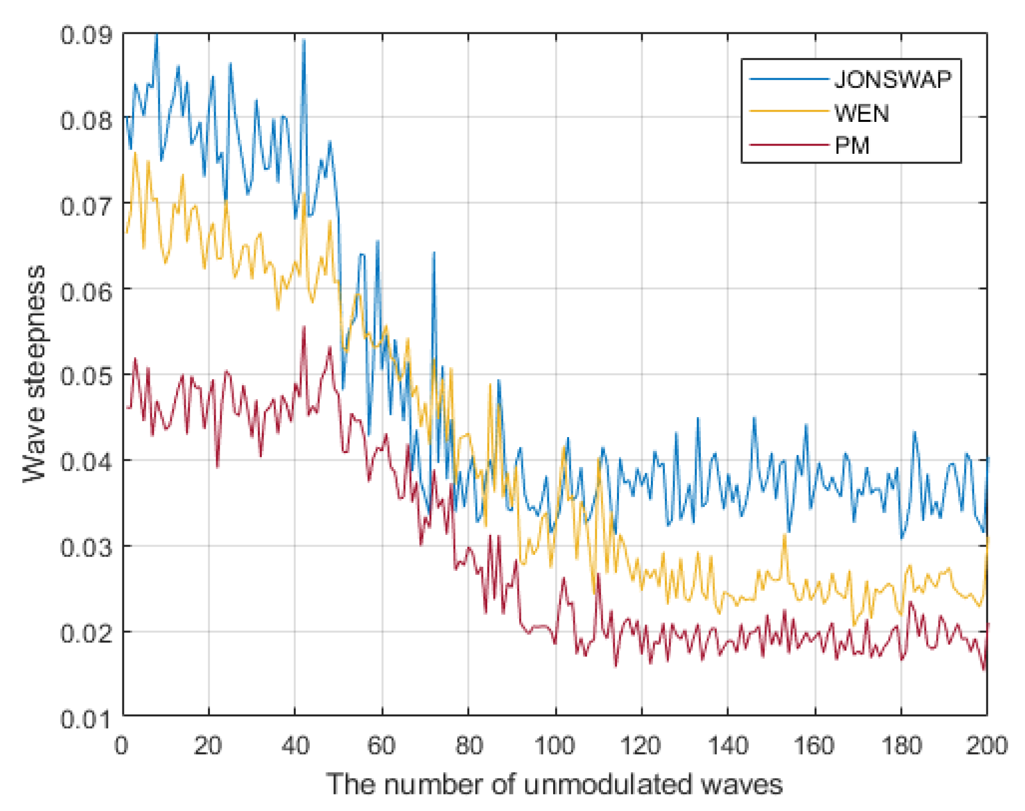
According to references [39,40], given some conditions, such as one-way waves, the probability of freak waves will increase with the increase of wave steepness. In the process of determining the number of modulated waves, we refer to the important characteristic quantity in ocean engineering—wave steepness [41]. As the ratio of wave height and wavelength, wave steepness is difficult to measure directly in actual ocean engineering. Generally, period estimation is used, that is, , where is the wave height, is the acceleration of gravity, and is the period. The results of the variation of the wave steepness with the number of unmodulated waves for the three wave spectra are recorded in Figure 3.
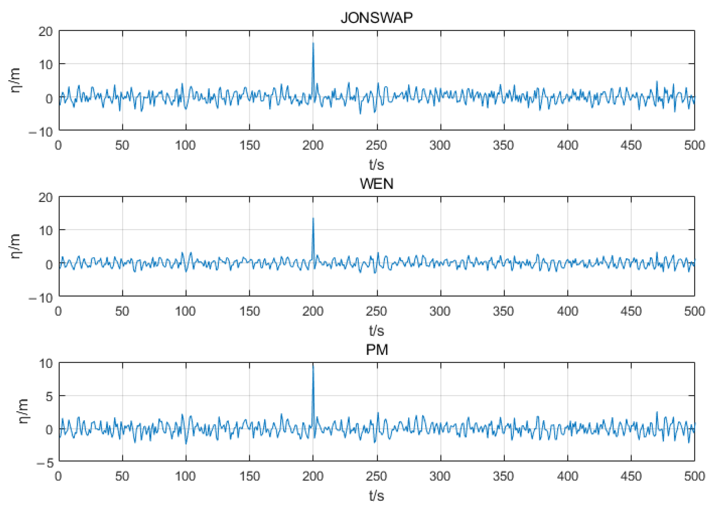
It can be seen from Figure 3 that the wave steepness of the three wave spectra shows a downward trend as a whole with the decrease in the number of modulated waves. The wave steepness is also larger when the number of modulated waves is larger, which also verifies that it is more reasonable to select a larger modulation interval in the previous experiments. Moreover, the wave steepness of the JONSWAP spectrum is generally larger than that of Wen’s spectrum and the PM spectrum. From the point of view of wave steepness, it is more appropriate to select the JONSWAP spectrum for the simulation of freak waves. In addition, considering the wave breaking when generating freak waves, Mori [42] has proved through a large number of experimental studies that when the wave steepness is less than 0.12, the wave is a non-breaking wave. It can be seen from Figure 3 that the wave steepness of the freak wave generated by the three wave spectra simulation will not produce wave breaking under each number of modulated waves, but as an extreme wave, the limit wave steepness of the freak wave remains to be discussed. According to the change of wave steepness, in the modulation interval 171–180 obtained from the above experiment, we select the number of modulated waves as 180 to simulate the time series of freak waves generated by the three wave spectra. The simulation results are recorded in Figure 4, and the wave characteristic parameters of the simulated freak waves are listed in Table 3.
From the comparison of the parameters in Table 3, it can be seen that the numerical calculation results of different wave spectra under this number of modulated waves all meet the definition of freak wave and the requirements of wave breaking. Through the comparison of characteristic parameters and the comparison of wave steepness of different wave spectra, it can be well proved that the feasibility of numerical simulation of the two-dimensional freak wave method and the accuracy of parameter selection in this paper, and the JONSWAP spectrum is more suitable for the simulation of freak waves.
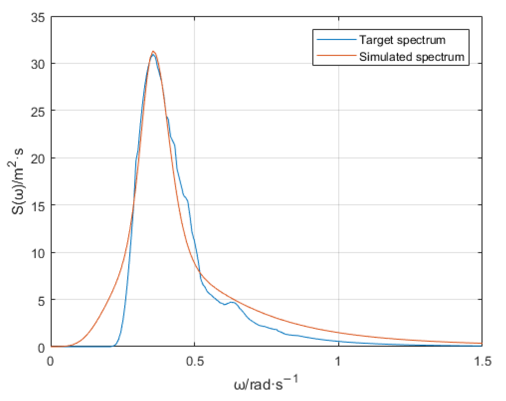
The most famous freak wave in history is the “New Year Wave” [43,44] that occurred in the Norwegian waters of the North Sea on January 1st, 1995, which was recorded by the Draupner jacket platform. According to the record, the freak wave occurred when the wave train t = 264.5 s. The characteristic parameters of the freak wave are a1 = 2.15, a2 = 0.72, a3 = 2.25, a4 = 3.99. The crest height is 18.50 m, the significant wave height is 11.92 m, and the maximum wave height is 25.60 m. Based on the above experimental results, we used the JONSWAP spectrum and selected the number of modulation waves to be 180 to simulate the “New Year Wave” and recorded the results of five experiments in Table 4. The time series of the first two numerical simulations of the “New Year Wave” are shown in Figure 5. In addition, we perform Fourier transform on the wave train of the “New Year Wave” to obtain the energy spectrum of the wave train and smooth it. We take this energy spectrum as the target spectrum and compare it with the energy spectrum of a numerical simulation. The results are shown in Figure 6.
For the time series of the New Year Wave, please refer to [43]. It can be seen from Figure 5 that the numerical simulation freak wave can be generated at a specific position. From the data in Table 4, it can be seen that the results of several numerical simulations of the “New Year Wave” are in good agreement with the measured data of the “New Year Wave”, and it can be seen from Figure 6 that the target spectrum and the simulated spectrum fit well. The above results can well illustrate that the improved phase modulation method obtained by comparing parameters is feasible.
3.2. Calculation and Analysis of Freak Wave Electromagnetic Scattering
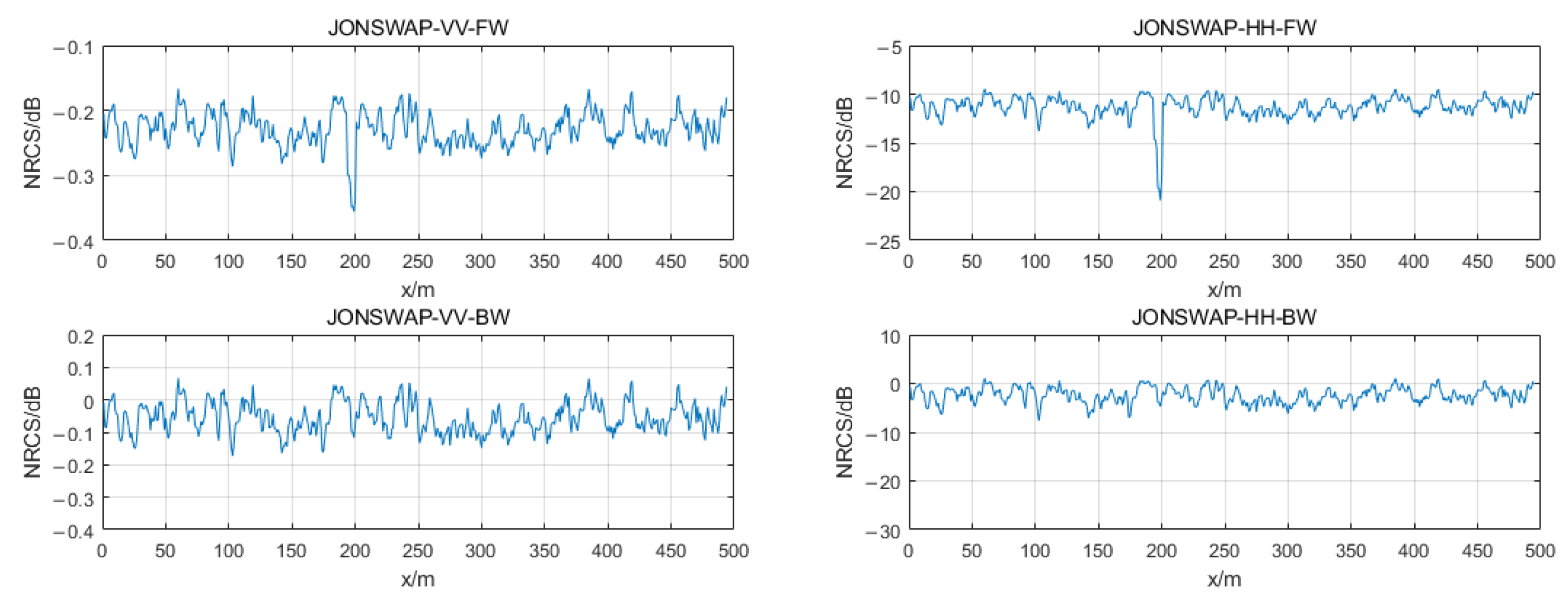
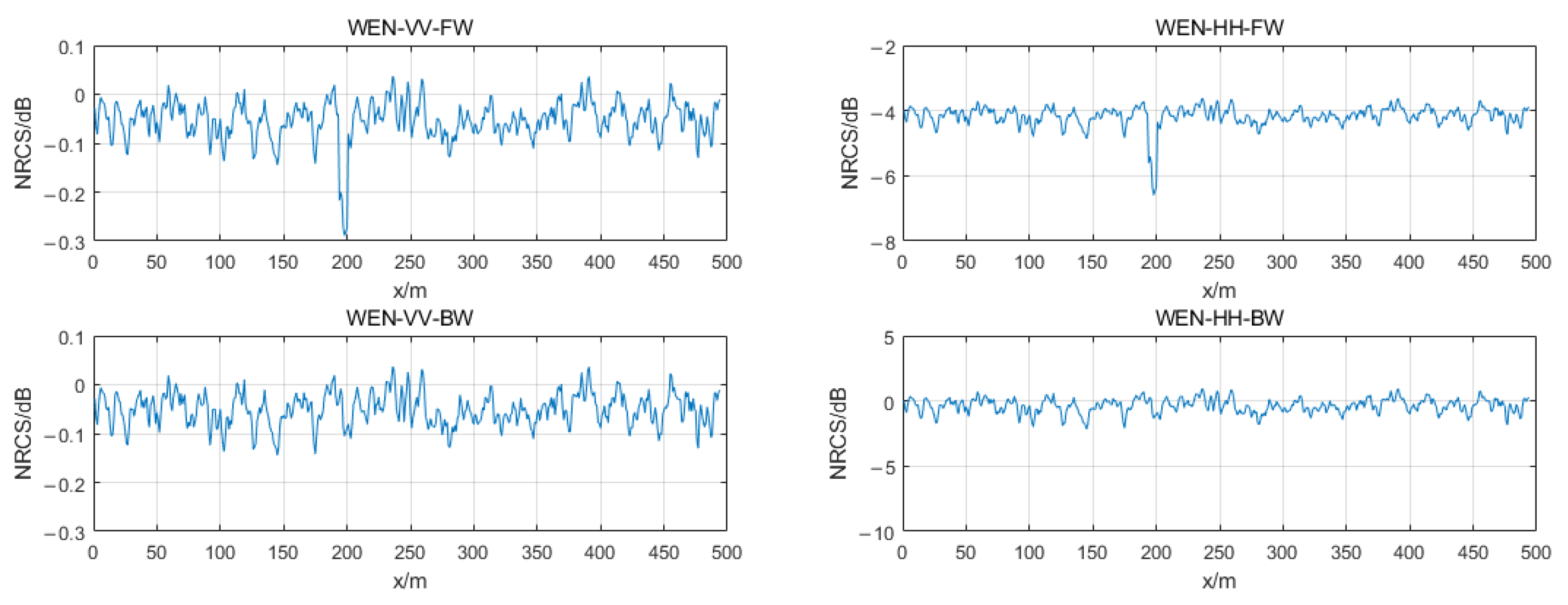
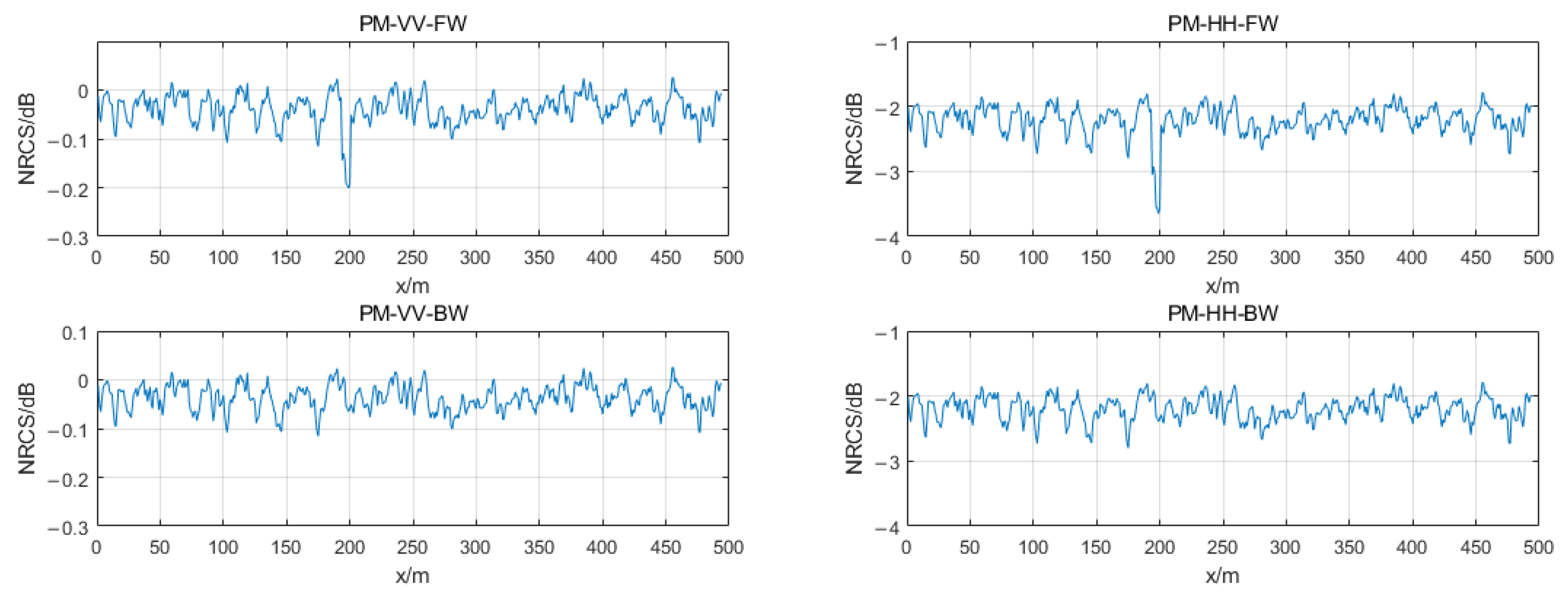
For rough seas, the normalized radar cross section (NRCS) is used to represent the electromagnetic scattering capability. The electromagnetic scattering characteristics of freak wave surfaces simulated by different wave spectra are studied. According to the experimental results of the freak wave numerical simulation, the number of constituent waves and the number of modulated waves are taken as 200 and 180, respectively, and the radar operating frequency is selected as , the incident angle is , the wind area is , the wind speed , and the relative azimuth angle is , the dielectric constant of seawater is 81. Generally, the echo strength of cross-polarization ( and ) is much lower than that of co-polarization ( and ). So in the study of electromagnetic scattering, we usually use polarization and polarization. We select three wave spectra, compare the two polarization modes of and , and calculate the electromagnetic scattering coefficient of the simulated freak wave. The results are shown in Figure 7, Figure 8, and Figure 9.
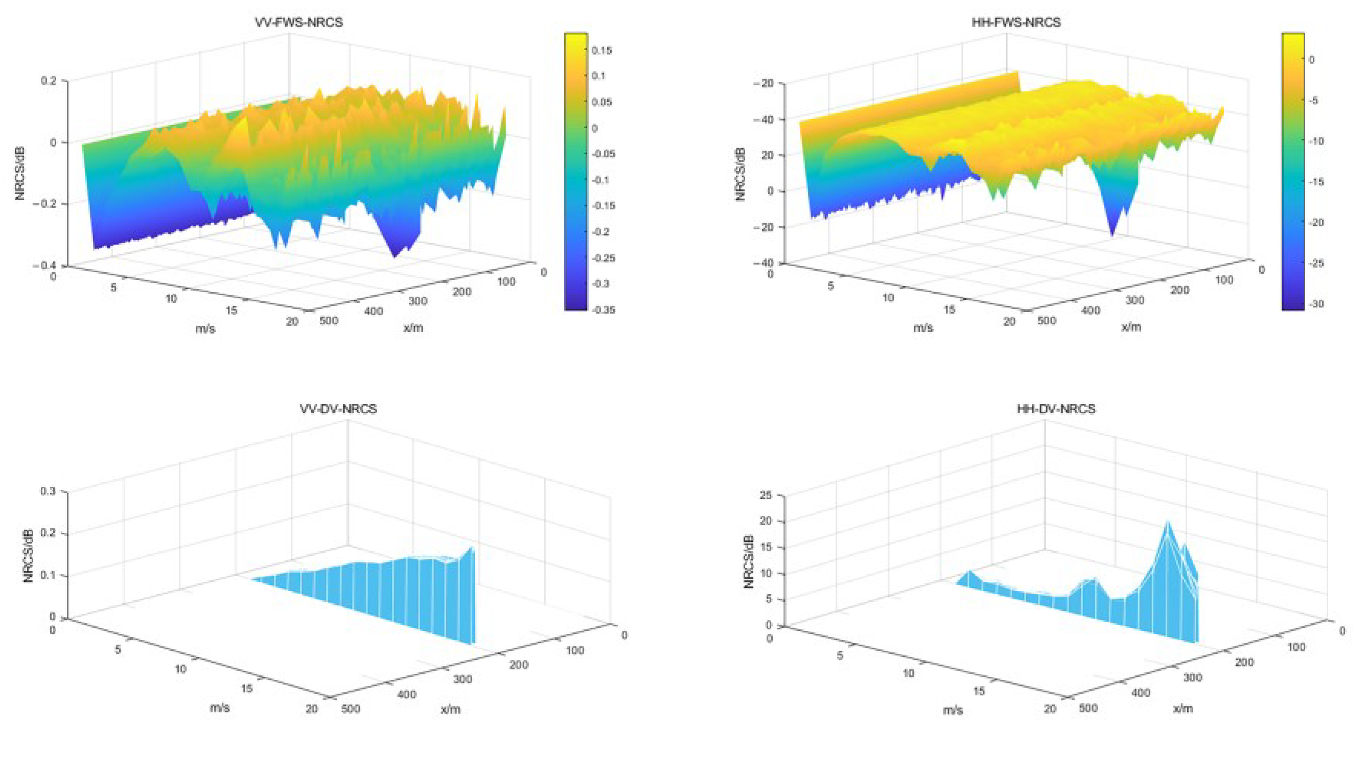
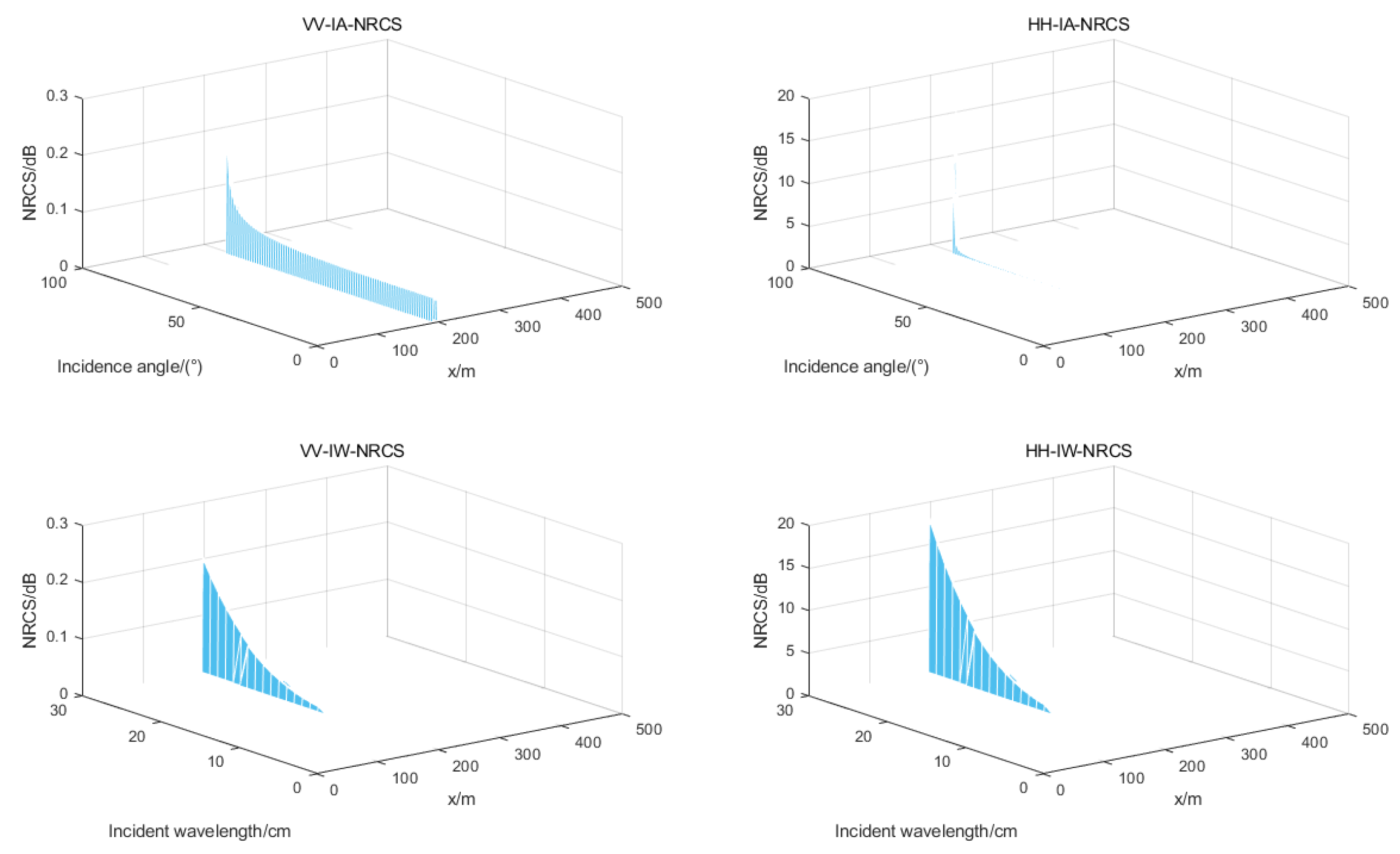
From the analysis of the experimental results, it can be seen that the scattering characteristics of the freak wave and its background wave are basically the same. The NRCS reaches a minimum value at the trough position and a maximum value at the peak position, and the NRCS is significantly lower than the background wave at the position where the freak wave is generated. As an extreme wave, a freak wave will change the incident plane from sea level to the plane along the freak wave where it is generated so that part of the energy of the wave whose phase is opposite and whose wavelength amplitude meets certain conditions is offset, resulting in the reduction of the scattering coefficient. In the polarization mode, the NRCS of the JONSWAP spectrum reaches the minimum value of at the location where the freak wave is generated, which is different from the NRCS of the background wave; the NRCS of Wen’s spectrum reaches the minimum value of at the location where the freak wave is generated, which is different with the NRCS of the background wave; the NRCS of the PM spectrum reaches the minimum value of at the location where the freak wave is generated, which is different with the NRCS of the background wave. It can be seen from the comparison that the difference value of NRCS of the JONSWAP spectrum is significantly larger than that of the other two wave spectra. The difference value of NRCS of the three wave spectra under the polarization mode is similar and significantly smaller than those under the polarization mode. This is consistent with the results of Kudryavtsev’s research [45] that NRCS under VV polarization is smaller than that under HH polarization. At the position where the freak wave appears, the transition of the electromagnetic scattering coefficient is not smooth because the actual sea surface is divided into different scales only according to the theory, which is different from the actual sea surface [46], so the TSM also has shortcomings. Based on the above experimental results, we studied the variation of NRCS of freak wave surface generated by the JONSWAP spectrum and the difference value of NRCS between freak wave and background wave with wind speed at the generation position of a freak wave under two polarization modes. We also studied the variation of the difference value of NRCS with incident angle and incident wavelength. The results are shown in Figure 10 and Figure 11.
It can be seen from Figure 10 that the NRCS of the freak wave surface first increases and then decreases with the increase of the wind speed , and the NRCS at the location where the freak wave was generated is obviously low. The difference value of NRCS of the two polarization modes increases with the increase of wind speed, and the difference value of NRCS of the polarization mode is significantly larger. It can be seen from Figure 11 that with the increase of the incident angle , the difference value of NRCS between a freak wave and a background wave under the two polarization modes are both increasing and show a significant increasing trend. This is because as the incident angle increases, the radar incident wave gradually approaches the angle parallel to the sea surface, and the NRCS is low. In the L-band range of the radar, the difference value of NRCS increases with the increase of the incident wavelength. We know that the incident wavelength is inversely proportional to the incident frequency. That is, the difference value of NRCS decreases with the increase of the incident frequency (the L-band corresponds to the incident frequency ), and the change trends of the two polarization modes are similar. Based on the above experimental analysis, the freak wave and the background wave have a relatively obvious NRCS difference, among which the difference under the JONSWAP spectrum and polarization is . Therefore, the difference value of NRCS can be used as an indicator of the freak wave detected by the radar. The above experiments only consider relatively ideal sea conditions. In practical situations, the influence of receiver noise, shadows, foam, etc., on the electromagnetic scattering results should also be considered. This is also where our future research needs to be improved.
4. Conclusions
In this paper, an improved phase modulation method is used to simulate a two-dimensional freak wave. Simulated freak waves can be generated at specific locations. In order to improve the accuracy and efficiency of numerical simulation, the simulation process is discussed from several aspects: the JONSWAP spectrum is more suitable for numerical simulation to generate freak waves than Wen’s spectrum and PM spectrum; when the number of constituent waves is 200 and the modulation interval is 171–180, the accuracy of numerical simulation is higher. The feasibility of our method is verified by spectral estimation. Combined with the numerical simulation results, we use the electromagnetic scattering calculation model based on TSM to study the electromagnetic scattering characteristics of the freak wave, and it is determined that the NRCS of the freak wave is different from that of the background wave. When the JONSWAP spectrum and polarization mode are selected, the difference value reaches . In addition, wind speed, incident angle, and incident frequency will have a significant impact on the scattering results. Considering the actual sea conditions, it is more convenient to calculate the difference value of NRCS of the freak wave than the parameters defined by the freak wave. Therefore, the difference value of NRCS can be considered as the identification mark of freak waves in practical engineering.
Author Contributions
All authors contributed to the research in this paper. Data curation, B.L.; formal analysis, G.W.; investigation, G.W.; methodology, L.H.; software, B.L.; writing—original draft, B.L.; writing—review and editing, G.W. All authors have read and agreed to the published version of the manuscript.
Funding
This research was funded by the Natural Science Foundation of Shandong Province, China, grant number ZR2021MD063.
Institutional Review Board Statement
Not applicable.
Informed Consent Statement
Not applicable.
Data Availability Statement
The raw data supporting the conclusions of this article will be made available by the authors, without undue reservation.
Conflicts of Interest
The authors declare no conflict of interest.
References
- Draper, L. Freak wave. Mar. Obs. 1965, 35, 193–195. [Google Scholar]
- Didenkulova, I.; Didenkulova, E.; Didenkulov, O. Freak wave accidents in 2019–2021. In Proceedings of the OCEANS 2022-Chennai, Chennai, India, 21–24 February 2022. [Google Scholar]
- Haver, S. Freak Waves: A Suggested Definition and Possible Consequences for Marine Structures, Rogue Waves: Brest, France, 20 October 2004.
- Residori, S.; Onorato, M.; Bortolozzo, U.; Arecchi, F. Rogue waves: A unique approach to multidisciplinary physics. Contemp. Phys. 2017, 58, 53–69. [Google Scholar] [CrossRef]
- Xu, P.; Du, Z.; Gong, S. Numerical Investigation into Freak Wave Effects on Deepwater Pipeline Installation. J. Mar. Sci. Eng. 2020, 8, 119. [Google Scholar] [CrossRef] [Green Version]
- Dysthe, K.; Krogstad, H.E.; Müller, P. Oceanic rogue waves. Annu. Rev. Fluid Mech. 2008, 40, 287–310. [Google Scholar] [CrossRef]
- Wang, Y.; Xu, F.; Zhang, Z. Numerical Simulation of Inline Forces on a Bottom-Mounted Circular Cylinder Under the Action of a Specific Freak Wave. Front. Mar. Sci. 2020, 7, 1149. [Google Scholar] [CrossRef]
- Gao, J.; Ma, X.; Zang, J.; Dong, G.; Ma, X.; Zhu, Y.; Zhou, L. Numerical investigation of harbor oscillations induced by focused transient wave groups. Coast. Eng. 2020, 158, 103670. [Google Scholar] [CrossRef]
- Fedele, F.; Brennan, J.; Ponce de León, S.; Dudley, J.; Dias, F. Real world ocean rogue waves explained without the modulational instability. Sci. Rep. 2016, 6, 27715. [Google Scholar] [CrossRef]
- Amrutha, M.M.; Sanil Kumar, V.; Anoop, T.R.; Nair, B.; Nherakkol, A.; Jeyakumar, C. Waves off Gopalpur, northern Bay of Bengal during cyclone Phailin. Ann. Geophys. 2014, 32, 1073–1083. [Google Scholar] [CrossRef] [Green Version]
- Zhang, H.; Yuan, Y.; Tang, W.; Xue, H.; Liu, J.; Qin, H. Numerical analysis on three-dimensional green water events induced by freak waves. Ships Offshore Struct. 2021, 16 (Suppl. S1), 33–43. [Google Scholar] [CrossRef]
- Zeng, F.; Zhang, N.; Huang, G.; Gu, Q.; Pan, W. A novel method in generating freak wave and modulating wave profile. Mar. Struct. 2022, 82, 103148. [Google Scholar] [CrossRef]
- Doong, D.-J.; Chen, S.-T.; Chen, Y.-C.; Tsai, C.-H. Operational Probabilistic Forecasting of Coastal Freak Waves by Using an Artificial Neural Network. J. Mar. Sci. Eng. 2020, 8, 165. [Google Scholar] [CrossRef]
- Cui, C.; Zhang, N.; Kang, H.; Yu, Y. An experimental and numerical study of the freak wave speed. Acta Oceanol. Sin. 2013, 32, 51–56. [Google Scholar] [CrossRef]
- Slunyaev, A.; Didenkulova, I.; Pelinovsky, E. Rogue waters. Contemp. Phys. 2011, 52, 571–590. [Google Scholar] [CrossRef]
- Chabchoub, A.; Hoffmann, N.; Onorato, M.; Akhmediev, N. Super rogue waves: Observation of a higher-order breather in water waves. Phys. Rev. X 2012, 2, 011015. [Google Scholar] [CrossRef] [Green Version]
- Clauss, G.; Stutz, K.; Schmittner, C. Rogue wave impact on offshore structures. In Proceedings of the Offshore Technology Conference, Houston, TX, USA, 3–6 May 2004. [Google Scholar]
- Clauss, G.F.; Schmittner, C.E.; Hennig, J.; Guedes Soares, C.; Fonseca, N.; Pascoal, R. Bending Moments of an FPSO in Rogue Waves. In Proceedings of the ASME 2004 23rd International Conference on Offshore Mechanics and Arctic Engineering, Vancouver, BC, Canada, 20–25 June 2004. [Google Scholar]
- Mansoori, A.; Desmond, D.; Stern, G.; Isleifson, D. Modeling Normalized Radar Cross-Section of Oil-contaminated Sea Ice with Small Perturbation Method. In Proceedings of the 2021 IEEE 19th International Symposium on Antenna Technology and Applied Electromagnetics (ANTEM), Winnipeg, MB, Canada, 8–11 August 2021; pp. 1–2. [Google Scholar]
- Wei, S.; Yang, S.; Xu, D. On accuracy of SAR wind speed retrieval in coastal area. Appl. Ocean Res. 2020, 95, 102012. [Google Scholar] [CrossRef]
- Schulz-Stellenfleth, J.; König, T.; Lehner, S. An empirical approach for the retrieval of integral ocean wave parameters from synthetic aperture radar data. J. Geophys. Res. Ocean. 2007, 112, 1–13. [Google Scholar] [CrossRef]
- Hopkin, M. Sea snapshots will map frequency of freak waves. Nature 2004, 430, 492–493. [Google Scholar] [CrossRef] [Green Version]
- Van Groesen, E.; Turnip, P.; Kurnia, R. High waves in Draupner seas—Part 1: Numerical simulations and characterization of the seas. J. Ocean Eng. Mar. Energy 2017, 3, 233–245. [Google Scholar] [CrossRef] [Green Version]
- Van Groesen, E.; Turnip, P.; Kurnia, R. High waves in Draupner seas—Part 2: Observation and prediction from synthetic radar images. J. Ocean Eng. Mar. Energy 2017, 3, 325–332. [Google Scholar] [CrossRef] [Green Version]
- Law, Y.Z.; Santo, H.; Chua, K.H. Wave-field prediction based on radar snapshots taken on a moving vessel. J. Phys. 2022, 2311, 012022. [Google Scholar] [CrossRef]
- Wijaya, A.P.; Naaijen, P.; Van Groesen, E. Reconstruction and future prediction of the sea surface from radar observations. Ocean Eng. 2015, 106, 261–270. [Google Scholar] [CrossRef]
- Hasselmann, D.; Dunckel, M.; Ewing, J. Directional Wave Spectra Observed during JONSWAP 1973. J. Phys. Oceanogr. 1980, 10, 1264–1280. [Google Scholar] [CrossRef]
- Bouws, E.; Günther, H.; Rosenthal, W.; Vincent, C.L. Similarity of the wind wave spectrum in finite depth water: 1. Spectral form. J. Geophys. Res. Ocean. 1985, 90, 975–986. [Google Scholar] [CrossRef]
- Bouws, E.; Günther, H.; Rosenthal, W.; Vincent, C.L. Similarity of the wind wave spectrum in finite depth water part 2: Statistical relations between shape and growth stage parameters. Dtsch. Hydrogr. Z. 1987, 40, 1–24. [Google Scholar] [CrossRef]
- Wen, S.; Guan, C.; Sun, S.; Wu, K.; Zhang, D. Effect of water depth on wind-wave frequency spectrum I. Spectral form. Chin. J. Oceanol. Limnol. 1996, 14, 97–105. [Google Scholar]
- Pierson, W.; Moskowitz, L. A proposed spectral form for fully developed wind seas based on the similarity theory of S. A. Kitaigorodskii. J. Geophys. Res. Atmos. 1964, 69, 5181–5190. [Google Scholar] [CrossRef]
- Longuet-Higgins, M. On the Statistical Distribution of the Heights of Sea Waves. J. Mar. Res. 1952, 11, 245–266. [Google Scholar]
- Wu, G.; Liang, Y.; Xu, S. Numerical computational modeling of random rough sea surface based on JONSWAP spectrum and Donelan directional function. Concurr. Comput. Pract. Exp. 2021, 33, 1–15. [Google Scholar] [CrossRef]
- Fung, A.; Lee, K. A semi-empirical sea-spectrum model for scattering coefficient estimation. IEEE J. Ocean. Eng. 1982, 7, 166–176. [Google Scholar] [CrossRef]
- Ulaby, F.T.; Moore, R.K.; Fung, A.K. Microwave Remote Sensing: Active and Passive. Volume III—From Theory to Applications; Artech House Inc.: London, UK, 1986; Volume 22, pp. 1223–1227.
- Holliday, D. Resolution of a controversy surrounding the Kirchhoff approach and the small perturbation method in rough surface scattering theory. IEEE Trans. Antennas Propag. 1987, 35, 120–122. [Google Scholar] [CrossRef]
- Li, D. Research on Electromagnetic Scattering Characteristics of Nonlinear Sea Surface. Ph.D. Thesis, University of Electronic Science and Technology of China, Chengdu, China, 2020. (In Chinese). [Google Scholar]
- Klinting, P.; Sand, S. Analysis of Prototype Freak Waves; ASCE: New York, NY, USA, 1987. [Google Scholar]
- Kim, D. On the Statistical Characteristics of Freak Wave Occurrence. J. Korean Soc. Mar. Environ. Eng. 2011, 14, 138–145. [Google Scholar] [CrossRef] [Green Version]
- Andrade, D.; Stuhlmeier, R.; Stiassnie, M. Freak waves caused by reflection. Coast. Eng. 2021, 170, 104004. [Google Scholar] [CrossRef]
- Kim, D. Statistical Analysis of Draupner Wave Data. J. Ocean Eng. Technol. 2019, 3, 252–258. [Google Scholar] [CrossRef]
- Mori, N. Effects of wave breaking on wave statistics for deep-water random wave train. Ocean Eng. 2003, 30, 205–220. [Google Scholar] [CrossRef]
- Haver, S. A possible freak wave event measured at the Draupner Jacket 1 January 1995. Rogue Waves 2004, 2004, 1–8. [Google Scholar]
- Clauss, G.F.; Klein, M. The New Year Wave: Spatial Evolution of an Extreme Sea State. J. Offshore Mech. Arct. Eng. 2009, 131, 041001. [Google Scholar] [CrossRef] [Green Version]
- Kudryavtsev, V.; Hauser, D.; Caudal, G.; Chapron, B. A semiempirical model of the normalized radar cross-section of the sea surface 1. Background model. J. Geophys. Res. Ocean. 2003, 108, FET 2-1-FET 2-24. [Google Scholar] [CrossRef]
- Wu, G.; Ji, G.; Ji, T.; Ren, H. Study of electromagnetic scattering from two-dimensional rough sea surface based on improved Wen’s spectrum. Acta Phys. Sin. 2014, 63, 134203. [Google Scholar]
Figure 1.
Simulated wave 1 and simulated wave 2 generated by JONSWAP spectrum based on phase modulation method.
Figure 1.
Simulated wave 1 and simulated wave 2 generated by JONSWAP spectrum based on phase modulation method.

Figure 2.
a1, a2, a3, a4 of freak waves generated by three wave spectra corresponding to different numbers of unmodulated waves under different numbers of constituent waves.
Figure 2.
a1, a2, a3, a4 of freak waves generated by three wave spectra corresponding to different numbers of unmodulated waves under different numbers of constituent waves.

Figure 3.
Wave steepness values of freak waves generated by different wave spectra for different numbers of unmodulated waves.
Figure 3.
Wave steepness values of freak waves generated by different wave spectra for different numbers of unmodulated waves.

Figure 4.
JONSWAP spectrum simulation freak wave time series, Wen’s spectrum simulation freak wave time series, and PM spectrum simulation freak wave time series based on phase modulation method.
Figure 4.
JONSWAP spectrum simulation freak wave time series, Wen’s spectrum simulation freak wave time series, and PM spectrum simulation freak wave time series based on phase modulation method.

Figure 5.
Numerical simulation of “The New Year Wave” wave train 1 and wave train 2.

Figure 6.
Comparison of simulated wave spectrum and target “New Year Wave” spectrum.

Figure 7.
Comparison of NRCS results of freak wave (FW) and its background wave (BW) simulated by JONSWAP spectrum under VV polarization and HH polarization.
Figure 7.
Comparison of NRCS results of freak wave (FW) and its background wave (BW) simulated by JONSWAP spectrum under VV polarization and HH polarization.

Figure 8.
Comparison of NRCS results of freak wave (FW) and its background wave (BW) simulated by Wen’s spectrum under VV polarization and HH polarization.
Figure 8.
Comparison of NRCS results of freak wave (FW) and its background wave (BW) simulated by Wen’s spectrum under VV polarization and HH polarization.

Figure 9.
Comparison of NRCS results of freak wave (FW) and its background wave (BW) simulated by PM spectrum under VV polarization and HH polarization.
Figure 9.
Comparison of NRCS results of freak wave (FW) and its background wave (BW) simulated by PM spectrum under VV polarization and HH polarization.

Figure 10.
NRCS of freak wave surface (FWS) and the variation of the difference value (DV) of NRCS with wind speed under two polarization modes.
Figure 10.
NRCS of freak wave surface (FWS) and the variation of the difference value (DV) of NRCS with wind speed under two polarization modes.

Figure 11.
Variation of the difference value of NRCS with incident angle (IA) and incident wavelength (IW) under two polarization modes.
Figure 11.
Variation of the difference value of NRCS with incident angle (IA) and incident wavelength (IW) under two polarization modes.


Table 1.
The number of freak wave basic indicators a1 and a2 under different numbers of constituent waves (“−”represents that the number is too small and will not be recorded temporarily).
Table 1.
The number of freak wave basic indicators a1 and a2 under different numbers of constituent waves (“−”represents that the number is too small and will not be recorded temporarily).
| M = 50 | M = 100 | M = 200 | M = 250 | |
|---|---|---|---|---|
| JONSWAP a1 | − | 27 | 56 | 66 |
| JONSWAP a2 | − | 51 | 108 | − |
| WEN a1 | 15 | 42 | 91 | 100 |
| WEN a2 | − | 67 | 136 | − |
| PM a1 | 10 | 38 | 82 | 100 |
| PM a2 | − | 62 | 127 | − |
Table 2.
The number of freak waves generated by the three wave spectra in different modulation intervals and the total number of generated freak waves in each interval.
Table 2.
The number of freak waves generated by the three wave spectra in different modulation intervals and the total number of generated freak waves in each interval.
| JONSWAP | WEN | PM | SUM | |
|---|---|---|---|---|
| (0–9) | 1078 | 1113 | 1089 | 3280 |
| (10–19) | 1065 | 1090 | 1102 | 3257 |
| (20–29) | 1085 | 1133 | 1092 | 3310 |
| (30–39) | 1063 | 1095 | 1084 | 3242 |
| (40–49) | 1080 | 1126 | 1110 | 3299 |
| (50–59) | 899 | 1111 | 1099 | 3109 |
| (60–69) | - | 1108 | 1080 | 2188 |
| (70–79) | - | 1065 | 990 | 2055 |
| (80–89) | - | 957 | - | 957 |
Table 3.
Characteristic parameter values of freak waves of three kinds of wave spectra.
| a1 | a2 | a3 | a4 | S | |
|---|---|---|---|---|---|
| JONSWAP | 2.8811 | 0.8729 | 6.1197 | 3.8265 | 0.0792 |
| WEN | 3.2140 | 0.9107 | 6.0411 | 4.4050 | 0.0620 |
| PM | 3.0242 | 0.9074 | 5.1363 | 4.0284 | 0.0445 |
Table 4.
Comparison of parameters between the measured “New Year Wave” and the numerical simulation “New Year Wave”.
Table 4.
Comparison of parameters between the measured “New Year Wave” and the numerical simulation “New Year Wave”.
| The New Year Wave | Experiment 1 | Experiment 2 | Experiment 3 | Experiment 4 | Experiment 5 | |
|---|---|---|---|---|---|---|
| a1 | 2.15 | 2.10 | 2.12 | 2.17 | 2.02 | 2.13 |
| a2 | 0.72 | 0.73 | 0.80 | 0.70 | 0.79 | 0.79 |
| a3 | 2.25 | 2.54 | 2.17 | 2.03 | 2.55 | 2.79 |
| a4 | 3.99 | 3.99 | 4.18 | 4.09 | 3. 69 | 3.65 |
| significant wave height | 11.92 | 11.98 | 11.36 | 12.08 | 12.37 | 12.33 |
| maximum wave height | 25.60 | 25.20 | 24.14 | 26.27 | 25.08 | 26.22 |
| wave crest height | 18.50 | 18.49 | 19.42 | 18.30 | 19.88 | 20.70 |
Publisher’s Note: MDPI stays neutral with regard to jurisdictional claims in published maps and institutional affiliations. |
© 2022 by the authors. Licensee MDPI, Basel, Switzerland. This article is an open access article distributed under the terms and conditions of the Creative Commons Attribution (CC BY) license (https://creativecommons.org/licenses/by/4.0/).
Share and Cite
MDPI and ACS Style
Wu, G.; Liu, B.; Han, L. Normalized Radar Scattering Section Simulation and Numerical Calculation of Freak Wave. J. Mar. Sci. Eng. 2022, 10, 1631. https://doi.org/10.3390/jmse10111631
AMA Style
Wu G, Liu B, Han L. Normalized Radar Scattering Section Simulation and Numerical Calculation of Freak Wave. Journal of Marine Science and Engineering. 2022; 10(11):1631. https://doi.org/10.3390/jmse10111631
Chicago/Turabian StyleWu, Gengkun, Bin Liu, and Lichen Han. 2022. "Normalized Radar Scattering Section Simulation and Numerical Calculation of Freak Wave" Journal of Marine Science and Engineering 10, no. 11: 1631. https://doi.org/10.3390/jmse10111631
Note that from the first issue of 2016, this journal uses article numbers instead of page numbers. See further details here.