Position Control of Heave Compensation for Offshore Cranes Based on a Particle Swarm Optimized Model Predictive Trajectory Path Controller

Abstract

The wave compensation system can be very useful in several naval applications. It can greatly reduce the relative irregular motion between the two ships when replenishment operations are performed, or between the ship and the offshore platform, which is caused by the waves. It is widely used in offshore operations, offshore cargo transfer, oil and gas exploitation, deep-sea mining, the hoisting and recovery of submersibles, etc. However, when a crane is used in a ship or moving platform, due to the influence of the hull, the crane load movement is similar to a space ball pendulum, which causes the heave displacement to show significant nonlinear motion characteristics. Moreover, the time delay of the detection mechanism and control error could result in untimely compensation, which deteriorates the performance. Consequently, this paper proposes one advanced prediction compensation method, namely Particle Swarm Optimized Model Predictive Trajectory Path controller (PSO−MPTP), which can improve the heave compensation performance. This method, which is based on Model Predictive Control (MPC), is firstly applied to the position servo system and takes into account the heave prediction and control effects simultaneously. The heave displacement of the crane load could be predicted in multiple steps in advance and used as the input of the position loop of the compensation machine. The achieved simulations show that the proposed controller has better prediction ability, higher control accuracy, and stronger robustness.

1. Introduction

Human maritime industrial activities have become more and more significant in recent years. Consequently, crane operation, an essential part of the offshore industry and offshore facility supply chain, becomes more and more important. However, the interference of waves will make the ship move with 6-Degrees of Freedom (DOF) (sway, surge, heave, roll, pitch, and yaw) and seriously affect offshore lifting and cargo shifting operations on ships due to the complicated ocean environment [1]. In particular, the heave motion and yaw motion have the most significant impact on the crane load during the operation process [2]. Due to other relatively small motions compared to the heave motion, heave compensation is the more crucial motion for the offshore work of cranes.

Normally, the basic principle of heave compensation is to use sensors to detect and record the relative distance of ship and crane load and produce a compensation signal to the crane to make the load swing at the opposite speed. In this way, a collision between the cargo and ship deck caused by waves can be avoided, and the safety of cargo operators during lifting work can be improved. If the heave motion of cranes could be predicted in advance and the servo system can effectively compensate over time, the unnecessary heave movement of the load can be significantly reduced [3].

The wave compensation system is generally divided into the Passive Heave Compensation system (PHC), Active Heave Compensation system (AHC), and Semi-Active Heave Compensation system (SAHC) [4]. In principle, the PHC device is located between the offshore crane and the crane load and can be represented by a parallel spring damping system. It does not require energy and is generally used with heavy loads and low accuracy requirements. PHC cannot compensate for the relative motion between the effective load and the ship in real-time, which has a specific time delay. To summarize, PHC has limitations in compensating for relative motion. The compensation efficiency of PHC in decoupling ship heave motion and load motion does not exceed 80% [5], while for AHC, the performance largely depends on the reliability of the control system. The relative compensated speed is much faster and the compensation accuracy is much higher. It can adjust the overcompensation more actively and significantly suppress the coupling of the heave motion of the payload [6]. However, this system consumes energy and is more suitable for small and medium-sized systems. SAHC combines the advantages of PHC and AHC, which can achieve satisfactory compensation accuracy with lower energy consumption [7]. Nevertheless, due to the combination of the two systems, SAHC is more complicated and expensive.

Huang et al. designed an AHC that satisfies the good control characteristics of the wave compensation system and obtains higher compensation accuracy [8]. The Motion Reference Unit (MRU) measures the actual ship motion. The AHC controller then calculates the motion of the actuator to counteract the ups and downs. The efficiency of the system can reach more than 90% [9,10]. The primary actuation of most AHCs is delivered by either hydraulic or electric drive systems. The electric drive system-based AHC has more advantages than the hydraulic system-based AHC in terms of compensation accuracy and speed. The efficiency of the electric heave compensation systems is between 70% and 80%. Compared with hydraulic systems, the characteristics of no oil reservoir and low motor noise have attracted more and more consumers. Moreover, for hydraulic systems in general, the biggest disadvantage is low efficiency with likely as low as 10% to 35% average efficiency of some open-loop systems [11].

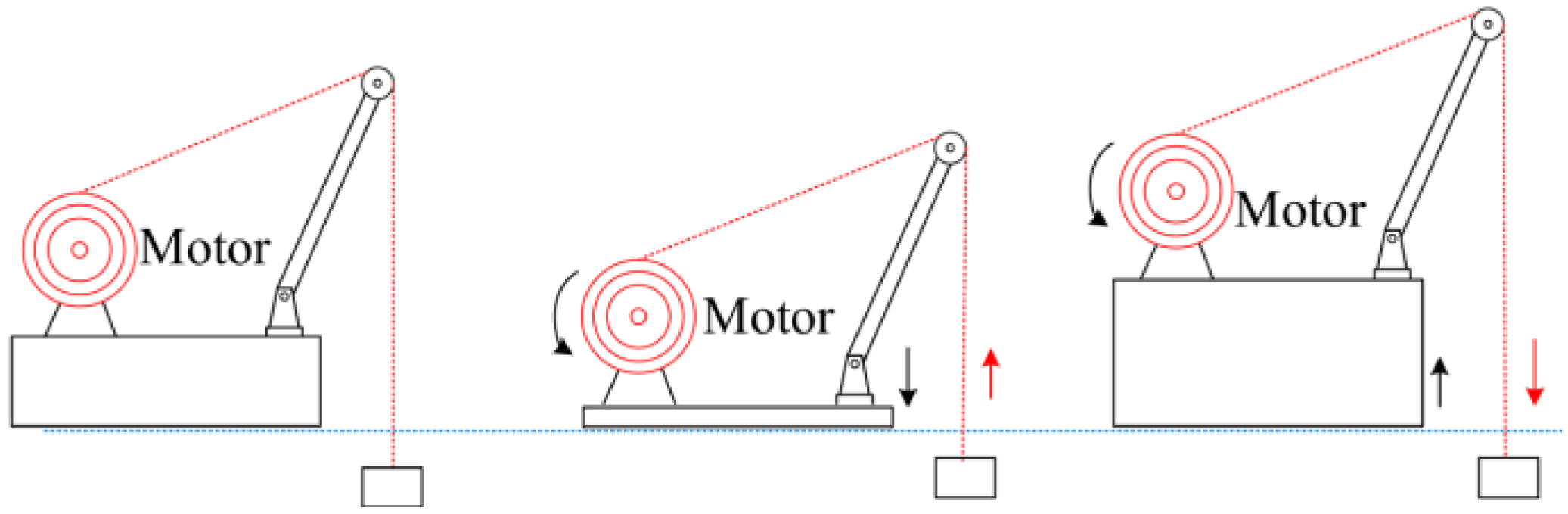
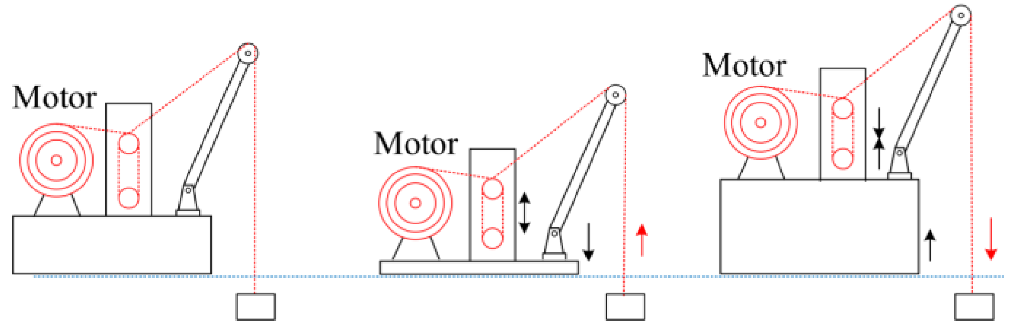
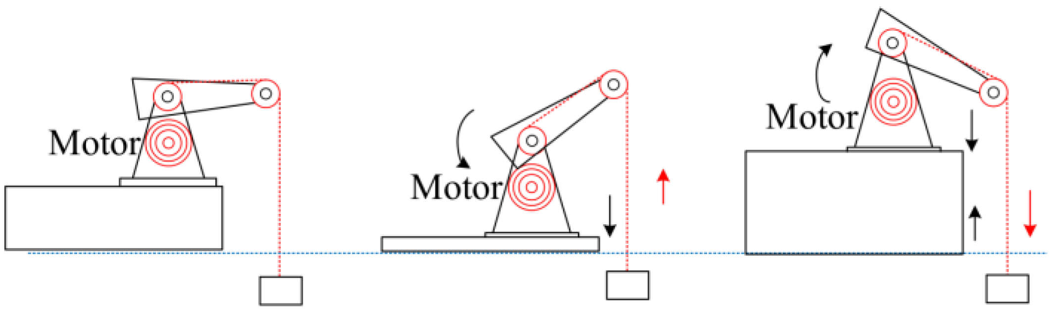
As shown in Figure 1, Figure 2 and Figure 3, AHCs are mainly divided into the draw-works retractable type, the hydraulic cylinder telescopic type, and the boom luffing type [12]. This paper will mainly focus on the draw-works retractable type, which is shown in Figure 1.

A number of papers have investigated AHC with the aim of reducing compensation errors. The most commonly used method is predicting the movement of the crane load and compensating for the prediction result. Lin et al. compensated for the heave motion of a crane based on motion prediction and fuzzy PID control [13]. Due to the hysteresis of the hydraulic system, it is difficult to respond quickly and accurately to the control signal. The compensation action and wave motion are out of step, which affects the compensation effect. The method proposed in Ref. [13] can not only solve the hysteresis, which has always existed in hydraulic actuators, but also uses motion prediction and fuzzy PID to avoid overshoot and instability. Chu et al. proposed a neural network-based ship motion prediction method to apply to offshore crane operations and implemented the proposed AHC algorithm [14]. They trained a multi-layer perceptron model to predict the ship’s motion and used the ship’s future motion information as the controller’s input to compensate for the shaking of the crane load. This method used predictive data for control and helped to overcome the signal delay of measuring sensor data. Longer forecasts can also provide on-board support and early warnings to prevent system failures. Neupert et al. used the prediction of heave motion as part of the AHC crane control method [15]. A crane dynamics-based linear model and a pole-assignment control method to set the load position were adopted. Shi et al. proposed a Kalman filter-based using Kalman Filter Particle Swarm Optimization to improve the prediction performance of a Support Vector Regression (KPSO-SVR) advanced statistical machine learning algorithm to analyze and research deep-sea fishing vessels [16]. Unlike the previous neural network algorithm, it can avoid the neural network over-fitting phenomenon that may occur due to the minimization of the Structural Risk Minimization (SRM ) structure risk to accurately predict the heave motion of the ship crane to compensate for the crane load. The proposed prediction model can overcome the increasing lag of the Autoregressive Moving Average Model (ARMA) prediction model over time. Küchler et al. proposed a prediction algorithm for the heave movement of crane load [17]. The Fast Fourier Transform (FFT) analyzes the motion caused by waves in the frequency domain. A peak detection algorithm extracts the amplitude, frequency, and other signals from the frequency domain signal, which is then processed by a Kalman filter. After the identification, the heave movement of the crane load is estimated. Using the controller and prediction method, which can significantly reduce the heave movement of the crane load, compensates for the dead time in the system.

High-precision compensation for the heave of the crane load is carried out using the control algorithm in the compensation mechanism. Cai, Zheng, and Liu proposed an adaptive robust dual-loop control scheme and proposed a multi-degree-of-freedom velocity feedforward compensator to decouple motion disturbances from the basic platform [18]. The original dynamic model was transformed into a linear parameterized form, and the adaptive law was used to estimate the basic parameters. A command-filter-based adaptive robust controller was developed to solve the problem that the uncertainty from the load and hydraulic system may reduce the system performance. Woodacre, Bauer, and Irani designed a Model Predictive Control (MPC) controller to drive a hydraulic test system for unloading and compared the experimental results of the PID controller [19]. It was found that the MPC controller can track various test cases and references and is better than the PID controller in all experiments. The decoupling of the transmitted movement by the MPC-PI controller can reduce the percentage by 99.6%. Johansen et al. combined the traditional AHC with the feedforward control strategy [20]. It reduced the impact force and effectively improved the stability of the crane load. Messineo and Serrani proposed an adaptive controller for heavy cranes [21]. It used an adaptive observer and two adaptive external interference models to make the closed-loop system adaptive in terms of equipment parameters and harmonic disturbance frequencies. Yang et al. designed a neural network-based adaptive control method to control the driving and non-driving state variables without any linearization operation [22]. In particular, the proposed rule could effectively compensate for the uncertainty of parameters and crane system structure. The manipulator and rope can reach the preset position within a limited time, and the payload swing can be suppressed entirely. Arnold et al. proposed a nonlinear control strategy combined with a model-based optimal trajectory generation method [23]. The trajectory tracking and anti-interference of crane load transportation were studied. The optimal control problem solved online considers the linearized system including state feedback, input, and state constraints. The generated optimal trajectory and straightness pitch motion control were applied to the measurement of the mobile port crane. The movement of the load was greatly compensated. Richter et al. proposed a real-time model predictive trajectory planner [24]. By predicting the vertical position and speed of the crane apex, the optimal control problem with the state constraints for each time step was solved online. A repetitive polynomial-based trajectory planner was used as a fallback strategy if the best control solution could not be found within the available time. If the optimization algorithm fails to find an efficient solution within the available time, continuity of control can be guaranteed.

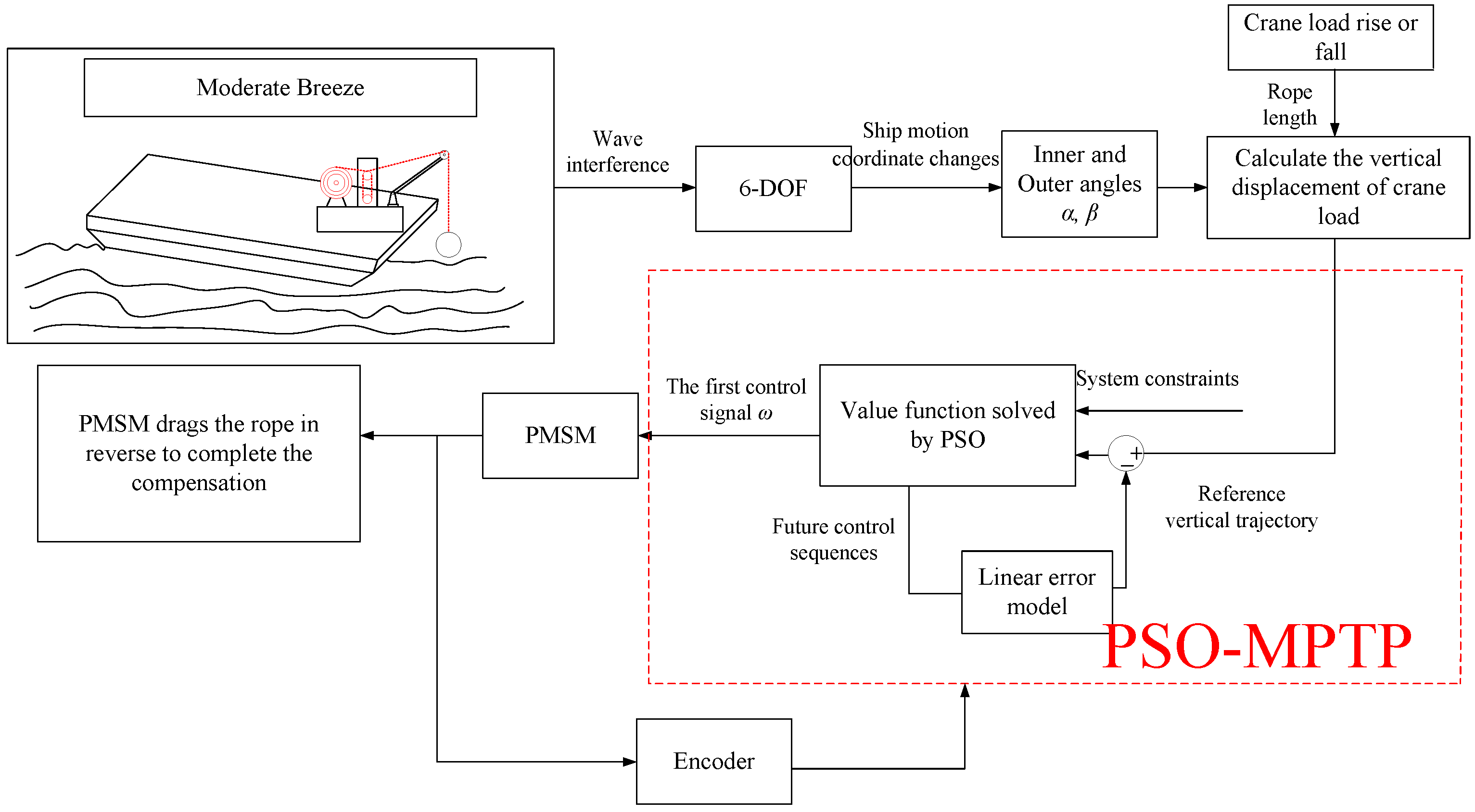
According to the literature, indeed, these references propose different methods, which could improve the compensation performance, using either feed-forward control to predict the heave motion or feedback control to compensate for the displacement of the crane load. However, these methods mainly focus on only one part and hardly discuss the hybrid control, which takes into account the prediction and control effects simultaneously to improve the performance. This paper proposes a Particle Swarm Optimized Model Predictive Trajectory Path (PSO−MPTP) controller, which combines the feed-forward and feedback controls. It uses the heave displacement trajectory signal of the crane load as an input to the compensation mechanism. Furthermore, according to this method, it can use future set-points to respond to changes in trajectory tracking in advance. This should be a good method to solve the above problems. For simplification, only the heave direction displacement of the crane load is considered. The trajectory of the crane load is tracked in the Northeast Down (NED) frame. The required reference trajectory is calculated, the actuator and measuring unit of the heave compensation system must be independent units of the modular platform. This paper adopts the Permanent Magnet Synchronous Motor (PMSM) servo system as the actuator in Figure 1, which is an important part of the offshore crane system. The PSO−MPTP is introduced into the wave compensation system for the first time, which replaces the conventional PI of the position loop in the three-phase closed-loop control of the traditional PMSM for real-time position compensation.

Consequently, this paper is structured as follows. In Section 2, the mathematical model of wave disturbance force and crane system is established. The overall system uses coordinate movement to obtain the displacement and velocity of the crane load in the heave direction. In Section 3, a mathematical model of PMSM is developed. In Section 4, the state equation is established for the motion equation of the crane system. Subsequently, PSO−MPTP for the position loop is designed and constrains the control quantity and control increment. Finally, the three-phase closed-loop control of the PMSM is presented and implemented in Matlab/Simulink. The analysis of the simulation results proves the feasibility of PSO−MPTP in the heave displacement compensation of the crane load.

2. System Model and Dynamic Equation

When the ship is traveling in the sea, it is affected by the wind and waves, which will cause the hull to shake and produce 6-DOF movement. The wave disturbance force is transmitted to the crane load through the hull, making the crane load heave and move. The overall process of the displacement compensation system of the crane load is shown in Figure 4.

The work in this article is based on some reasonable assumptions, which are as follows:

• Assuming that the shape of the crane ship is a square barge, the hull is regarded as a rigid body during operation and will not be deformed by the impact of waves. Moreover, during the lifting process, it is assumed that the sling is not deformed too much.
• The sling quality occupies a small proportion of the entire compensation system with negligible impact.
• Only the heave displacement of the crane load in the Z-axis direction is considered for compensation.

Firstly, the wave disturbance force is modeled. Waves on the sea surface are generated by the sea wind. The wind speed determines the height and period of each wave. The waves impact the hull, and the force is transmitted from the hull to the crane load subsequently.

According to the linear regression formula based on the data in the paper of Price and Bishop, the wave mathematical model is obtained in Formula (1) [25].

$$\{\begin{array}{l}a=0.015U_T^2+1.5\\ T_w=-0.0014U_T^3+0.042U_T^2+5.6\\ k={\omega }_k{}^2/g\end{array}$$

(1)

where a is the wave height (m); U_T is the wind speed (m/s); T_w is the wave period (s); k is the wave number; ω_k is the reciprocal of T_w.

Thus, the wave impact force and the corresponding torque can be calculated with Formulas (2) and (3) based on the hypothesis of Froude–Krylov [26].

$$\{\begin{array}{l}{F}_x=2\rho ga\frac{\sin \left[\left(kB/2\right)\sin \phi \right]}{\left(kB/2\right)\sin \phi }{e}^{-kd}Bd\sin \left[\left(k{L}_{ship}/2\right)\cos \phi \right]\sin {\omega }_{n}t\\ F_y=-2\rho ga\frac{\sin \left[\left(kB/2\right)\cos \phi \right]}{\left(kB/2\right)\cos \phi }{e}^{-kd}{L}_{ship}\sin \left[\left(kB/2\right)\sin \phi \right]\sin {\omega }_{n}t\\ F_z=\rho gak\frac{\sin \left[\left(kB/2\right)\sin \phi \right]}{\left(kB/2\right)\sin \phi }{e}^{-kd}Bd{L}_{ship}\frac{\sin \left[\left(kB/2\right)\cos \phi \right]}{\left(kB/2\right)\cos \phi }\cos {\omega }_{n}t\end{array}$$

(2)

$$\{\begin{array}{l}{M}_x=\rho ga\frac{\sin \left[\left(kB/2\right)\sin \phi \right]}{\left(kB/2\right)\sin \phi }{e}^{-kd}\sin \phi \frac{d^2\sin \left[\left(k{L}_{ship}/2\right)\cos \phi \right]}{\cos \phi }\sin {\omega }_{n}t\\ \begin{array}{l}{M}_y=\rho ga\frac{\sin \left[\left(kB/2\right)\sin \phi \right]}{\left(kB/2\right)\sin \phi }{e}^{-kd}d•\\ \frac{2\sin \left[\left(k{L}_{ship}/2\right)\cos \phi \right]-k{L}_{ship}\cos \phi \cos \left[\left(k{L}_{ship}/2\right)\cos \phi \right]}{k^2{\cos }^2\phi }\sin {\omega }_{n}t\end{array}\\ \begin{array}{l}{M}_z=\rho ga\frac{\sin \left[\left(kB/2\right)\sin \phi \right]}{\left(kB/2\right)\sin \phi }{e}^{-kd}\sin \phi •\\ \frac{2\sin \left[\left(k{L}_{ship}/2\right)\cos \phi \right]-k{L}_{ship}\cos \phi \cos \left[\left(k{L}_{ship}/2\right)\cos \phi \right]}{k^2{\cos }^2\phi }\cos {\omega }_{n}t\end{array}\end{array}$$

(3)

where F_x, F_y, and F_z are the wave force in x, y, and z directions of the hull (N); M_x, M_y, and M_z are the torque corresponding to the wave force in x, y, and z directions of the hull (N·m); ρ is the density of seawater (kg/m³); g is the gravitational acceleration (m²/s); d is the draft (m); B is the width of the ship (m); L_ship is the length of the ship’s waterline (m); φ is the wave encounter angle (rad); and ω_n is the encounter frequency (Hz). t is time and the above formula changes with time.

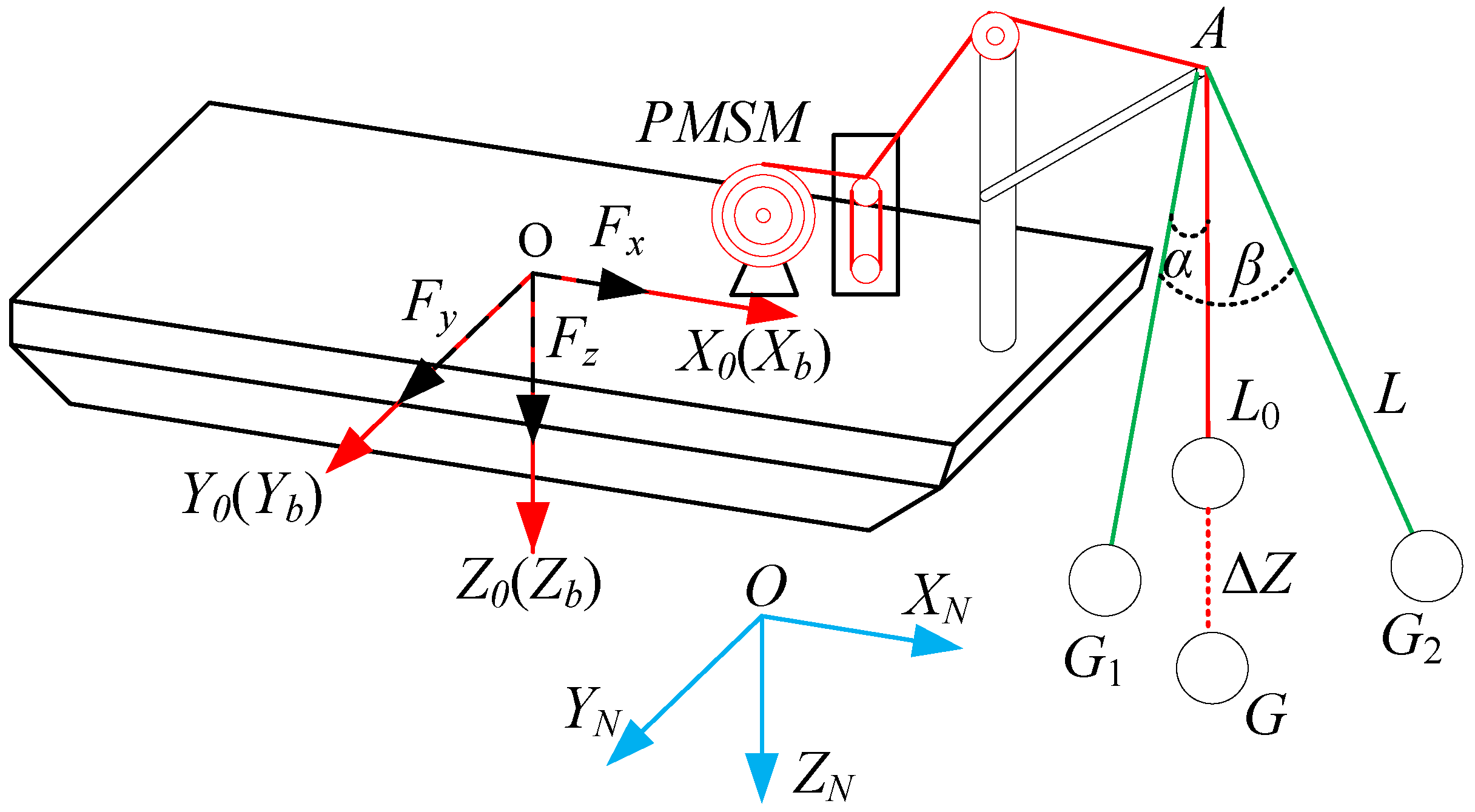
Figure 5 presents the ship crane system model. From this figure, A is the hoisting point, L₀ is the initial rope length of the hoisting rope, L is the rope length after the lifting and sinking displacement of the hoisting object, and α and β are the inner and outer angles of the plane. O-X_bY_bZ_b is the BODY (Body-axis coordinate system) frame, and O-X_NY_NZ_N is the NED (Northeast Down) frame. F_x, F_y, and F_z are wave forces. ΔZ is the heave displacement of the crane load.

The movement formula of the crane load in the system can be obtained in Formula (4).

$$\{\begin{array}{l}{x}_G(t)=x_A(t)+L\cos \alpha \cos \beta \\ y_G(t)=y_A(t)-L\sin \beta \\ z_G(t)=z_A(t)+L\cos \alpha \cos \beta \end{array}$$

(4)

Taking the first derivative of Formula (4), the speed of the crane load in three directions can be obtained in the following Formula (5).

$$\{\begin{array}{l}\stackrel{•}{x_G}(t)=\stackrel{•}{x_A}(t)+\stackrel{•}{L}\sin \alpha \cos \beta +\stackrel{•}{\alpha }L\cos \alpha \cos \beta -\stackrel{•}{\beta }L\sin \alpha \cos \beta \\ {\stackrel{•}{y}}_G(t)={\stackrel{•}{y}}_A(t)-\stackrel{•}{L}\sin \beta +\stackrel{•}{\beta }L\cos \beta \\ \stackrel{•}{z_G}(t)=\stackrel{•}{z_A}(t)+\stackrel{•}{L}\cos \alpha \cos \beta -\stackrel{•}{\alpha }L\sin \alpha \cos \beta -\stackrel{•}{\beta }L\cos \alpha \cos \beta \end{array}$$

(5)

According to Figure 5, when the crane load swings from the point G to point G₁, the potential energy of the Y_NOZ_N surface is set to 0 at this time, and the total kinetic energy and potential energy of the crane system can be deduced in Formula (6).

$$\{\begin{array}{l}T=\frac{1}{2}m{\stackrel{•}{x_G}}^2(t)+\frac{1}{2}m{\stackrel{•}{y_G}}^2(t)+\frac{1}{2}m{\stackrel{•}{z_G}}^2(t)\\ V=-mgl\cos \alpha \cos \beta \end{array}$$

(6)

Then, the Lagrangian function L_a of the crane load can be developed in Formula (7).

$$\begin{array}{l}{L}_a=T-V\\ =\frac{1}{2}{m}_G(\stackrel{•}{x_A{}^2}+\stackrel{•}{y_A{}^2}+\stackrel{•}{z_A{}^2}+\stackrel{•}{L^2}+L^2\stackrel{•}{{\alpha }^2}{\cos }^2\beta +L^2\stackrel{•}{{\beta }^2})+\\ m_G\stackrel{•}{x_p}(\stackrel{•}{L}\sin \alpha \sin \beta +\stackrel{•}{\alpha }L\cos \alpha \cos \beta -\stackrel{•}{\beta }L\sin \alpha \sin \beta )-\\ m_G\stackrel{•}{y_p}(\stackrel{•}{L}\sin \beta +\stackrel{•}{\beta }L\cos \alpha )+\\ m_G\stackrel{•}{z_p}(\stackrel{•}{L}\cos \alpha \cos \beta -\stackrel{•}{\alpha }L\sin \alpha \cos \beta -\stackrel{•}{\beta }L\cos \alpha \sin \beta )+\\ m_{G}gL\cos \alpha \cos \beta \end{array}$$

(7)

where m_G is the weight of the crane load (kg).

Using Formulas (2) and (3), combined with Newton’s second law, the acceleration of the wave force on the hull in the x, y, and z directions can be obtained. Then, according to the Lagrangian Equation (8), the second-order multivariate dynamic differential equation of the crane system can be obtained in Formula (9). The inner angle α and the outer angle β can be obtained by Formula (9).

$$\begin{gathered} \frac{d}{dt}\left(\frac{\partial L_a}{\partial \stackrel{•}{\alpha }}\right)-\left(\frac{\partial L_a}{\partial \alpha }\right)=0 \\ \frac{d}{dt}\left(\frac{\partial L_a}{\partial \stackrel{•}{\beta }}\right)-\left(\frac{\partial L_a}{\partial \beta }\right)=0 \end{gathered}$$

(8)

$$\begin{array}{l}\stackrel{••}{\alpha }\cos \beta -2\stackrel{•}{\alpha }\stackrel{•}{\beta }\sin \beta +\frac{g}{L}\sin \alpha +\frac{\stackrel{••}{x_p}}{L}\cos \alpha -\frac{\stackrel{••}{z_p}}{L}\sin \alpha +\frac{2\stackrel{•}{\alpha }\stackrel{•}{L}}{L}=0\\ \stackrel{••}{\beta }+\stackrel{•}{{\alpha }^2}\sin \beta \cos \beta +\frac{g}{L}\cos \alpha \sin \beta -\frac{\stackrel{••}{x_p}}{L}\sin \alpha \sin \beta -\frac{\stackrel{••}{y_p}}{L}\cos \beta -\frac{\stackrel{••}{z_p}}{L}\cos \alpha \sin \beta +\frac{2\stackrel{•}{\beta }\stackrel{•}{L}}{L}=0\end{array}$$

(9)

Finally, the heave displacement ΔZ of the crane load in the heave direction can be obtained in Formula (10) in accordance with the inner and outer angles and Figure 5.

$$\Delta Z=L\cos \alpha \cos \beta -L$$

(10)

ΔZ is the reference trajectory given by the heave motion of the crane load. The input is ΔZ to PSO−MPTP. Through PMSM three-phase closed-loop control, using the idea of trajectory tracking, with the help of the servo mechanism, PMSM can reverse track the heave displacement of ΔZ to maintain the position of the crane load.

3. Mathematical Model of PMSM

Due to the high torque-to-current ratio, high power-to-weight ratio, high efficiency, high power factor, and robustness, PMSM is adopted as the actuator of the servo mechanism in this paper, and the accuracy of motor control directly affects the efficiency of system compensation.

The voltage and flux expressions of PMSM in the dq axis are given in Formulas (11) and (12).

$$\{\begin{array}{c}{u}_d=L_d\frac{\mathrm{d}{i}_d}{\mathrm{d}t}+R_s{i}_d-{\omega }_e{\psi }_q\\ u_q=L_q\frac{\mathrm{d}{i}_q}{\mathrm{d}t}+R_s{i}_q+{\omega }_e{\psi }_d\end{array}$$

(11)

$$\{\begin{array}{l}{\psi }_d=L_d{i}_d+{\psi }_f\\ {\psi }_q=L_q{i}_q\end{array}$$

(12)

where u_d and u_q are the d and q-axis voltages (V); and i_d and i_q are the d and q -axis currents (A); L_d and L_q are the d and q-axis inductances (mH); ψ_d and ψ_q are the flux linkage components (Wb); R_s is the stator equivalent resistance (Ω), ω_e is the electrical angular velocity of the motor (rad/s); ψ_f is the permanent magnet flux of the rotor (Wb).

The torque equation is shown in Formula (13).

$$T_e=\frac{3}{2}{p}_n\left({\psi }_d{i}_q-{\psi }_q{i}_d\right)$$

(13)

The mechanical equation of the motor is given in Formula (14)

$$J\frac{\mathrm{d}{\omega }_m}{\mathrm{d}t}=T_e-T_L$$

(14)

where T_e is the electromagnetic torque (N·m); p_n is the number of pole pairs; J is the moment of inertia (kg·m²); ω_m is the mechanical angular velocity (rad/s); and T_L is the load torque (N·m).

4. Application of PSO−MPTP in Motor Position Control

The PID controller plays a leading role in industrial process control. However, because of the complicated working condition on the sea, the conventional PID controller has poor robustness and control performance to the parameters’ variation in the PMSM position servo system [27]. Moreover, the PID controller has other problems such as error selection, side effects of integral feedback, extraction of differential terms, and so on [28]. In order to overcome these disadvantages, Active Disturbance Rejection Control (ADRC) is proposed. They are all error-based controllers to eliminate error and do not need an accurate mathematical model. Although the performance of ADRC is better than PID [29], the traditional ADRC also has some problems in the PMSM position servo system, such as a slow positioning response, poor positioning accuracy, and difficult parameter setting [30]. For the sake of solving the defects of the above controllers, MPTP, which is developed from MPC, is proposed. The only difference is the initial state. For MPC, the initial state of the optimal control problem is the current feedback value of the control system. Based on the research background of this paper, the initial state of the optimal control problem for MPTP is the value calculated in advance. Thus, this section uses the PSO algorithm to increase the accuracy and speed of MPTP quadratic programming.

The PSO−MPTP is adopted in the position loop of three-phase closed-loop control of PMSM. In principle, the crane load position signal is used as the input of the position loop of the three-phase closed-loop of PMSM. After comparing it with the feedback position, the predicted desired speed can be obtained through PSO−MPTP and tracked by classical speed and current loops. According to this basic process, the compensated motor could rotate to drag the hoisting rope and compensate for the crane load in the heave direction, which can significantly reduce the wave disturbance and keep the crane load and the ship relatively static. In order to achieve this result, several steps should be followed.

4.1. Forecast Model Heading

To establish the relationship between heave displacement and the motor, the heave displacement ΔZ caused by the shaking of the crane load should be transformed into the rotation angle of the compensated motor in Formula (15). It means that the heave displacement can be controlled by the rotation of the compensated motor.

$$\theta =\frac{180}{\pi r}\Delta Z$$

(15)

where r is the radius of the roll (m).

The kinematic equation of the crane load at point G in the NED frame is presented in Formula (16).

$$\stackrel{•}{\theta }=\omega \cos \alpha \cos \beta$$

(16)

The expected displacement of the crane load is θ_r, the subscript r represents the reference quantity, and the actual displacement of the crane load is θ_m. The expected displacement error of the crane system can be summarized in Formula (17).

$$e\left(t\right)={\theta }_r\left(t\right)-{\theta }_m\left(t\right)$$

(17)

The desired displacement error should be as small as possible. Therefore, the limitation of e(t) is zero in Formula (18).

$$\underset{t\to \infty }{\lim }e(t)=0$$

(18)

It can be seen from Formula (16) that the entire crane system can be regarded as a control system with a state quantity of θ = [θ_m] and a control quantity of W = [ω_m]. Its general form can be represented by Formula (19).

$$\stackrel{•}{\theta }=f(\theta ,W)$$

(19)

At each moment, the jitter caused by the wave disturbance force on the crane load satisfies the above kinematic equation. It can be summarized in Formula (20).

$${\stackrel{•}{\theta }}_r=f({\theta }_r,W_r)$$

(20)

After the Taylor series expansion of Formula (19), it can be rewritten in Formula (21) if the higher-order terms are ignored.

$$\stackrel{•}{\theta }=f({\theta }_r,W_r)+\frac{\partial f(\theta ,W)}{\partial \theta }|{}_{\begin{array}{l}\theta ={\theta }_r\\ W=W_r\end{array}}(\theta -{\theta }_r)+\frac{\partial f(\theta ,W)}{\partial W}|{}_{\begin{array}{l}\theta ={\theta }_r\\ W=W_r\end{array}}(W-W_r)$$

(21)

The state quantity deviation and control quantity deviation of the crane system are assumed to be represented by Formula (22).

$$\begin{array}{l}\tilde{\theta }=[{\stackrel{•}{\theta }}_m-\stackrel{•}{{\theta }_r}]\\ \tilde{W}=[{\omega }_m-\stackrel{}{{\omega }_r}]\end{array}$$

(22)

The combination of Formulas (21) and (20) gives Formula (23).

$$\tilde{\theta }=\left[{\stackrel{•}{\theta }}_m-{\stackrel{•}{\theta }}_r\right]=\cos \alpha \cos \beta \left[{\omega }_m-{\omega }_r\right]$$

(23)

Formula (23), based on the kinematics model, needs to be discretized to obtain the discrete state space Formula (24).

$$\tilde{\theta }(k+1)=[1]\tilde{\theta }(k)+[T\cos \alpha \cos \beta ]\tilde{W}(k)$$

(24)

Formula (24) can be written in the form of Formula (25).

$$\tilde{\theta }(k+1)=a_k\tilde{\theta }(k)+b_k\tilde{W}(k)$$

(25)

With:

$$a_k=[1],b_k=[T\cos \alpha \cos \beta ]$$

In the value function, it is necessary to constrain the control increment to calculate the system’s output for a period of time in the future. Formula (25) is transformed into Formula (26).

$$\vartheta (k)=\left[\begin{array}{c}\tilde{\theta }(k)\\ \tilde{W}(k-1)\end{array}\right]$$

(26)

Formula (26) can be developed into expression Formulas (27) and (28) by recursion.

$$\vartheta (k+1)={\tilde{a}}_k\vartheta (k)+{\tilde{b}}_k\Delta \tilde{W}(k)$$

(27)

$$\theta (k)={\tilde{c}}_k\vartheta (k)$$

(28)

With:

$${\tilde{a}}_k=\left[\begin{array}{cc}{a}_k& b_k\\ 0_{m\times n}& I_m\end{array}\right],{\tilde{b}}_k=\left[\begin{array}{c}{b}_k\\ I_m\end{array}\right],{\tilde{c}}_k=\left[\begin{array}{cc}{I}_m& 0_{n\times n}\end{array}\right]$$

where m is the dimension of the state quantity; n is the dimension of the control quantity.

4.2. Rolling Optimization

From the calculation of (22)–(28), it can be seen that the prediction output expression of the system is Formula (29).

$$\mathrm{Y}(k)={\mathsf{\Psi }}_k\vartheta (k)+{\mathsf{\Phi }}_k\Delta W(k)$$

(29)

With:

$$\mathrm{Y}(k)=\left[\begin{array}{c}\tilde{\theta }(k+1)\\ \tilde{\theta }(k+2)\\ \dots \\ \tilde{\theta }(k+N_c)\\ \dots \\ \tilde{\theta }(k+N_p)\end{array}\right]$$

$${\mathsf{\Phi }}_k=\left[\begin{array}{cccc}{\tilde{c}}_k{\tilde{b}}_k& 0& \cdots & 0\\ {\tilde{c}}_k{\tilde{a}}_k{\tilde{b}}_k& {\tilde{c}}_k{\tilde{b}}_k& \cdots & 0\\ \cdots & \cdots & \ddots & ⋮\\ {\tilde{c}}_k{\tilde{a}}_k{}^{N_c-1}{\tilde{b}}_k& {\tilde{c}}_k{\tilde{a}}_k{}^{N_c-2}{\tilde{b}}_k& \cdots & {\tilde{c}}_k{\tilde{b}}_k\\ ⋮& ⋮& \ddots & ⋮\\ {\tilde{c}}_k{\tilde{a}}_k{}^{N_p-1}{\tilde{b}}_k& {\tilde{c}}_k{\tilde{a}}_k{}^{N_p-2}{\tilde{b}}_k& \cdots & {\tilde{c}}_k{\tilde{a}}_k{}^{N_p-N_c}{\tilde{b}}_k\end{array}\right]$$

$$\Delta W(k)=\left[\begin{array}{c}\Delta \tilde{W}(k)\\ \Delta \tilde{W}(k+1)\\ \cdots \\ \Delta \tilde{W}(k+N_c-1)\end{array}\right]$$

where N_p is the prediction time domain; N_c is the control time domain. Therefore, if the current state quantity and the control increment in the control time domain N_c are known, the system output in the future forecast time domain N_p can be predicted.

4.3. Rolling Optimization

For the value function to ensure that the suspension rope of the compensation motor can quickly and smoothly track the expected displacement of the crane load, it is necessary to optimize the deviation of the system state quantity and the control increment. This paper uses a value function of the form Formula (30) [31]:

$$J(k)={\displaystyle \sum _{j=1}^N{\tilde{\theta }}^T}(k+j)Q\tilde{\theta }(k+j)+\Delta {\tilde{W}}^T(k+j-1)R\Delta \tilde{W}(k+j-1)$$

(30)

where Q and R are symmetric positive definite weight matrices.

In Formula (30), the control quantity is used as the state quantity in the value function. The structure is simple and easy to realize, but it also has some shortcomings. It cannot accurately constrain the control increment, and the phenomenon of sudden changes in the control quantity of the controlled system is unavoidable. It seriously affects the continuity of the control amount. In this case, the control increment is selected as the state quantity of the value function, and Formula (31) is selected as the value function.

$$J(k)={{\displaystyle \sum _{i=1}^{N_p}\Vert {\theta }_m(k+i)-{\theta }_r(k+i)\Vert }}_{\overline{Q}}^2+{{\displaystyle \sum _{i=1}^{N_c-1}\Vert \Delta \tilde{W}(k+i)\Vert }}_{\overline{R}}^2$$

(31)

The first item of the value function represents the error between the output value and the reference value, reflecting the system’s ability to track the displacement of the reference crane load stably. The last item reflects the stability of the system’s control of the crane load. The whole function minimization will lead the system to track the expected displacement of the crane load quickly and stably. This will be performed acting in the compensation motor. The value optimization function problem shown in Formula (31) can be transformed into a quadratic programming problem through some processing.

At the same time, in the actual crane system, the speed and speed increment of the lifting and lowering of the crane load can only be limited within a specific range, and it cannot be increased infinitely. It is not only necessary to select the optimal value function but also to meet some constraints related to the state quantity and control quantity of the crane system, such as Formulas (32) and (33).

Control constraint:

$$W_{\min }(k+T)\le W(k+T)\le W_{\max }(k+T)\mathrm{with}:T=0,1,...,N_c–1$$

(32)

Control increment constraint:

$$\Delta W_{\min }(k+T)\le \Delta W(k+T)\le \Delta W_{\max }(k+T)\mathrm{with}:T=0,1,...,N_c–1$$

(33)

4.4. MPTP Optimal Solution Problem Based on PSO

In the value function, the control increment is a variable requiring solution, and the control increment constraint must be added to it. Therefore, the control constraint must be converted into the control increment constraint. The control quantity and control increment are given in the recursive Formula (34).

$$\begin{array}{ll}\hfill \tilde{W}(k)& =\tilde{W}(k-1)+\Delta \tilde{W}(k)\\ \hfill \tilde{W}(k+1)& =\tilde{W}(k)+\Delta \tilde{W}(k+1)\\ & =\tilde{W}(k-1)+\Delta \tilde{W}(k)+\Delta \tilde{W}(k+1)\\ & \cdots \\ \hfill \tilde{W}(k+N_c-1)& =\tilde{W}(k+N_c-2)+\Delta \tilde{W}(k+N_c-1)\\ & =\tilde{W}(k-1)+\Delta \tilde{W}(k)+\Delta \tilde{W}(k+1)+\cdots +\Delta \tilde{W}(k+N_c-1)\end{array}$$

(34)

The above formula can be rewritten as Formula (35).

$$\begin{array}{l}\left[\begin{array}{c}\tilde{W}(k)\\ \tilde{W}(k+1)\\ \tilde{W}(k+2)\\ \cdots \\ \tilde{W}(k+N_c-1)\end{array}\right]=\left[\begin{array}{c}\tilde{W}(k-1)\\ \tilde{W}(k-1)\\ \tilde{W}(k-1)\\ \cdots \\ \tilde{W}(k-1)\end{array}\right]+M\left[\begin{array}{c}\Delta \tilde{W}(k)\\ \Delta \tilde{W}(k+1)\\ \Delta \tilde{W}(k+2)\\ \cdots \\ \Delta \tilde{W}(k+N_c-1)\end{array}\right]\\ =W_k+M\Delta W(k)\end{array}$$

(35)

With:

$$M={\left[\begin{array}{ccccc}1& 0& \cdots & \cdots & 0\\ 1& 1& 0& \cdots & 0\\ 1& 1& 1& \ddots & 0\\ ⋮& ⋮& \ddots & \ddots & 0\\ 1& 1& \cdots & 1& 1\end{array}\right]}_{N_c\times N_c}\otimes I_{N_u}$$

where $I_{N_u}$ represents the unit matrix with dimension N_u, and $\otimes$ represents the Kronecker product.

In summary, we convert Formula (35) into Formula (36):

$$\begin{array}{l}{W}_{\min }=\left[\begin{array}{c}{\tilde{W}}_{\min }\\ {\tilde{W}}_{\min }\\ {\tilde{W}}_{\min }\\ \cdots \\ {\tilde{W}}_{\min }\end{array}\right]\le \left[\begin{array}{c}\tilde{W}(k)\\ \tilde{W}(k+1)\\ \tilde{W}(k+2)\\ \cdots \\ \tilde{W}(k+N_c-1)\end{array}\right]\le \left[\begin{array}{c}{\tilde{W}}_{\max }\\ {\tilde{W}}_{\max }\\ {\tilde{W}}_{\max }\\ \cdots \\ {\tilde{W}}_{\max }\end{array}\right]=W_{\max }\\ \Rightarrow W_{\min }\le W_k+M\Delta W(k)\le W_{\max }\end{array}$$

(36)

In the actual situation, the constraint amount should be defined clearly and given in Formula (37). In this paper, the set amount is selected only to verify the feasibility of the algorithm to constrain the control amount and control variable, it can be adjusted according to the actual situation.

$$\{\begin{array}{l}-1m/s\le W\le 1m/s\\ -0.5m/s\le \Delta W\le 0.5m/s\end{array}$$

(37)

Combining the Formulas (29) and (31), the complete value function can be achieved in Formula (38).

$$J(k)=\Delta W{(k)}^T{H}_k\Delta W(k)+2G_k{}^T\Delta W(k)$$

(38)

where $H_k={\mathsf{\Phi }}_k^{T}Q{\mathsf{\Phi }}_k+R$; $E={\mathsf{\Psi }}_k\vartheta (k)$; $G_k=E^{T}Q{\mathsf{\Phi }}_k$; H_k and G_k are positive definite matrices.

Finally, the MPTP optimal solution problem could be solved by PSO as in Formula (39). In fact, there may be other meta-heuristic optimization algorithms that are effective or better for MPTP, such as Firefly Algorithm (FA), the Genetic Algorithm (GA), and Ant Colony Optimization (ACO), etc. [32,33,34].

$$\begin{array}{l}\underset{\Delta W}{\min }\frac{1}{2}\Delta W{(k)}^T{H}_k\Delta W(k)+G_k^T\Delta W(k)\\ s.t.\{\begin{array}{c}{W}_{\min }\le W_k+M\Delta W(k)\le W_{\max }\\ \Delta W_{\min }\le \Delta W\le \Delta W_{\max }\end{array}\end{array}$$

(39)

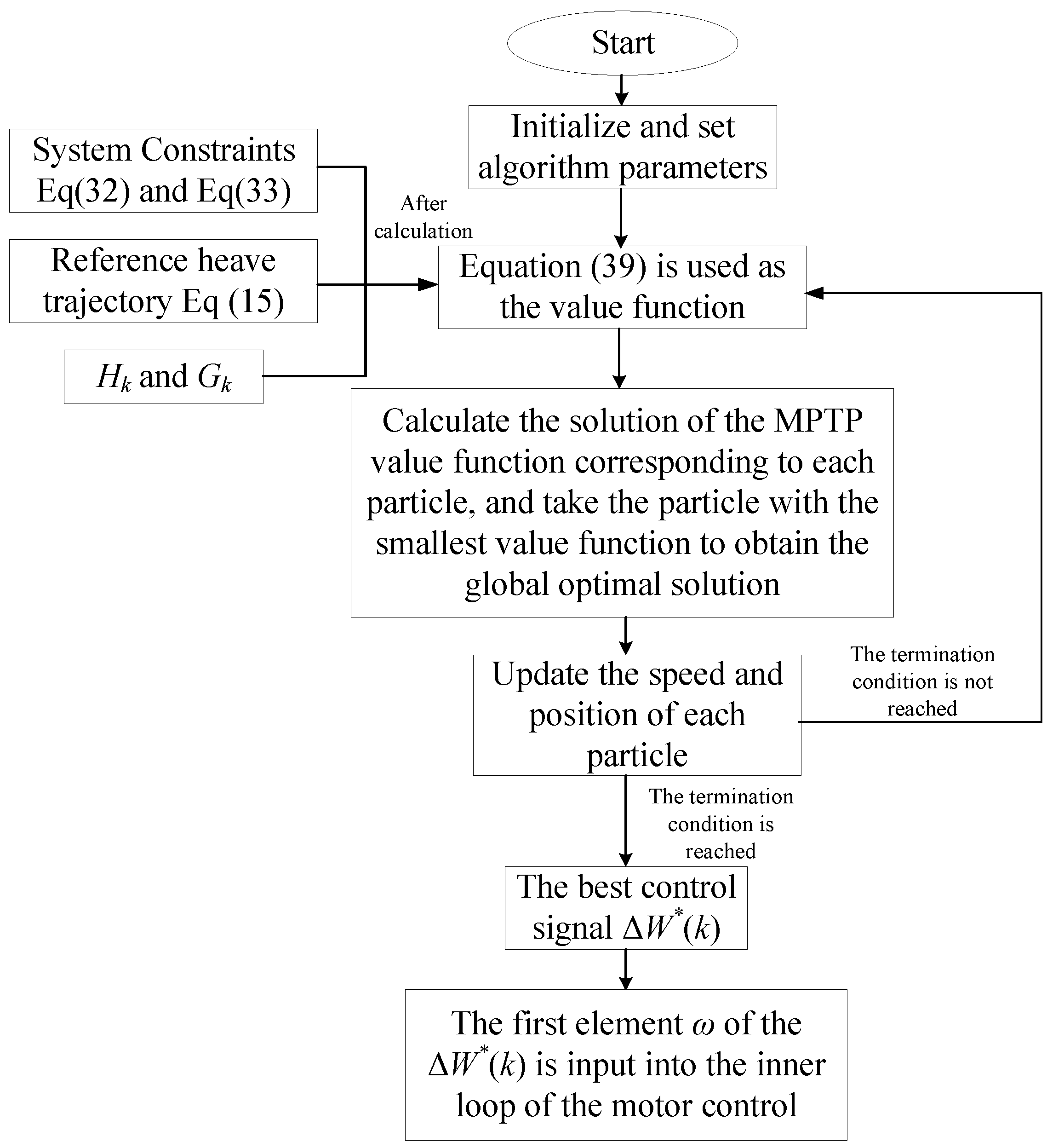
This basic optimization process is shown in Figure 6. Formula (39), as the value function of PSO, calculates the solution of the MPTP value function corresponding to each particle, and takes the particle with the smallest value function to obtain the global optimal solution.

According to Figure 6, after solving each control cycle, a series of control input increments $\Delta W^{\ast }(k)=\left[\begin{array}{cccc}\Delta {\omega }^{\ast }(k)& \Delta {\omega }^{\ast }(k+1)& \dots & \Delta {\omega }^{\ast }(k+N_c-1)\end{array}\right]$ can be obtained. The first element of the control sequence is the input in the inner loop of the motor control as the actual increment. Finally, the predicted angular velocity output value of the compensation motor at time k can be expressed as Formula (40).

$$\omega (k)=\omega (k-1)+\Delta {\omega }^{\ast }(k)$$

(40)

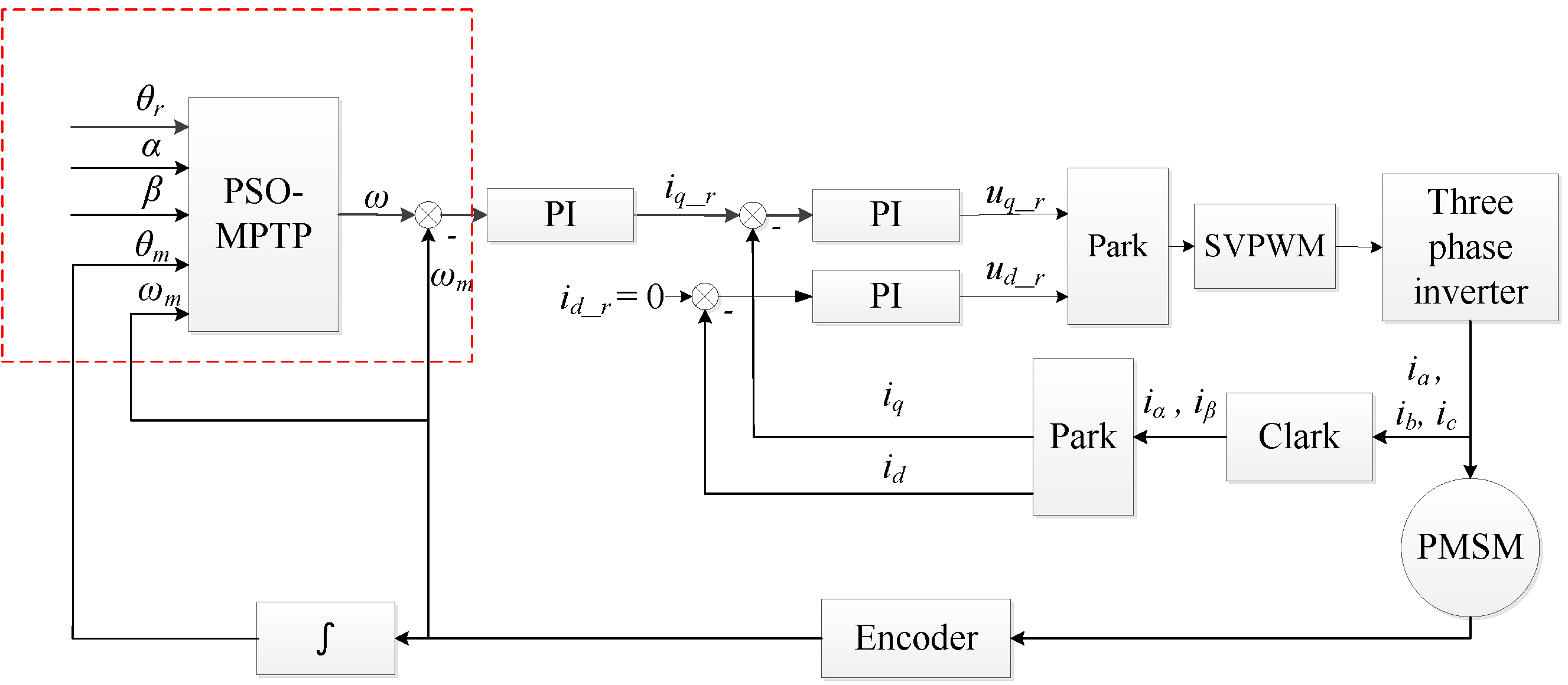
At each moment, the predicted angular velocity is cyclically input into the PI controller of the motor speed loop, and then input into the current loop. Finally, the actual output value of the compensation motor angle can be obtained, which will be fed back to the position loop PSO−MPTP. The system will continue to start the prediction work at the next moment. The three-phase closed-loop control of the motor is shown in Figure 7.

5. Simulation Result Heading

In order to compare and analyze the results objectively, the evaluation coefficient should be defined. According to the literature and applicable situation, the evaluation coefficient Compensation Efficiency (CE), used for evaluating the compensation effect, is finally selected and defined in Formula (41) [35,36,37].

CE = [1 − std(d)/std(h)] × 100%

(41)

where d is the error after compensation, h is the displacement in the heave direction of the ship, and std is the standard deviation.

The prediction time domain N_p = 20 and the control time domain N_c = 1 are chosen for multi-step prediction of the crane load’s position. All the simulation results are compared with that of conventional PI and ADRC, which are achieved according to [38,39]. In this paper, the compensation displacement is inverted in Simulink to facilitate comparison with ΔZ.

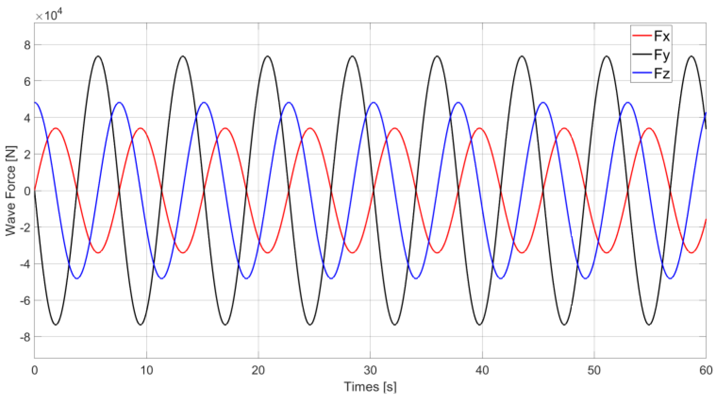
The background of this article is that regular waves are in a level 4 sea state: U_T = 8 m/s, and φ = 45°. Wave force simulation results are shown in Figure 8.

5.1. Simulation under Ideal Conditions

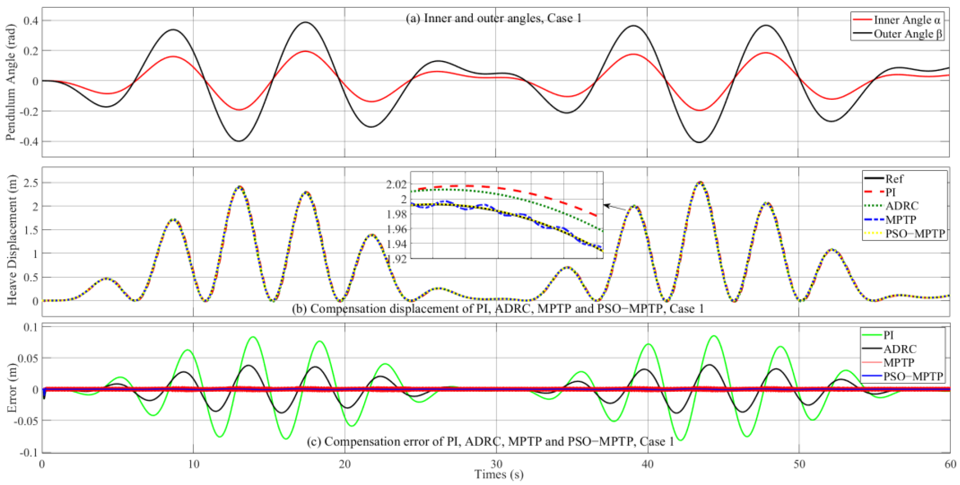
Case 1: L = 25 m and V = 0 m/s

In this case, the crane load hovers. It can be seen from Figure 9 that the inner and outer angles are not large, and the maximum displacement of the crane load in the heave direction is approximately 2.5 m. The CE of PI is 95.7%, the CE of ADRC is 98.1%, the CE of MPTP is 99.3%, and the CE of PSO−MPTP is 99.7%. Consequently, the displacement of the crane load in the heave direction is significantly reduced, and PSO−MPTP has a better performance.

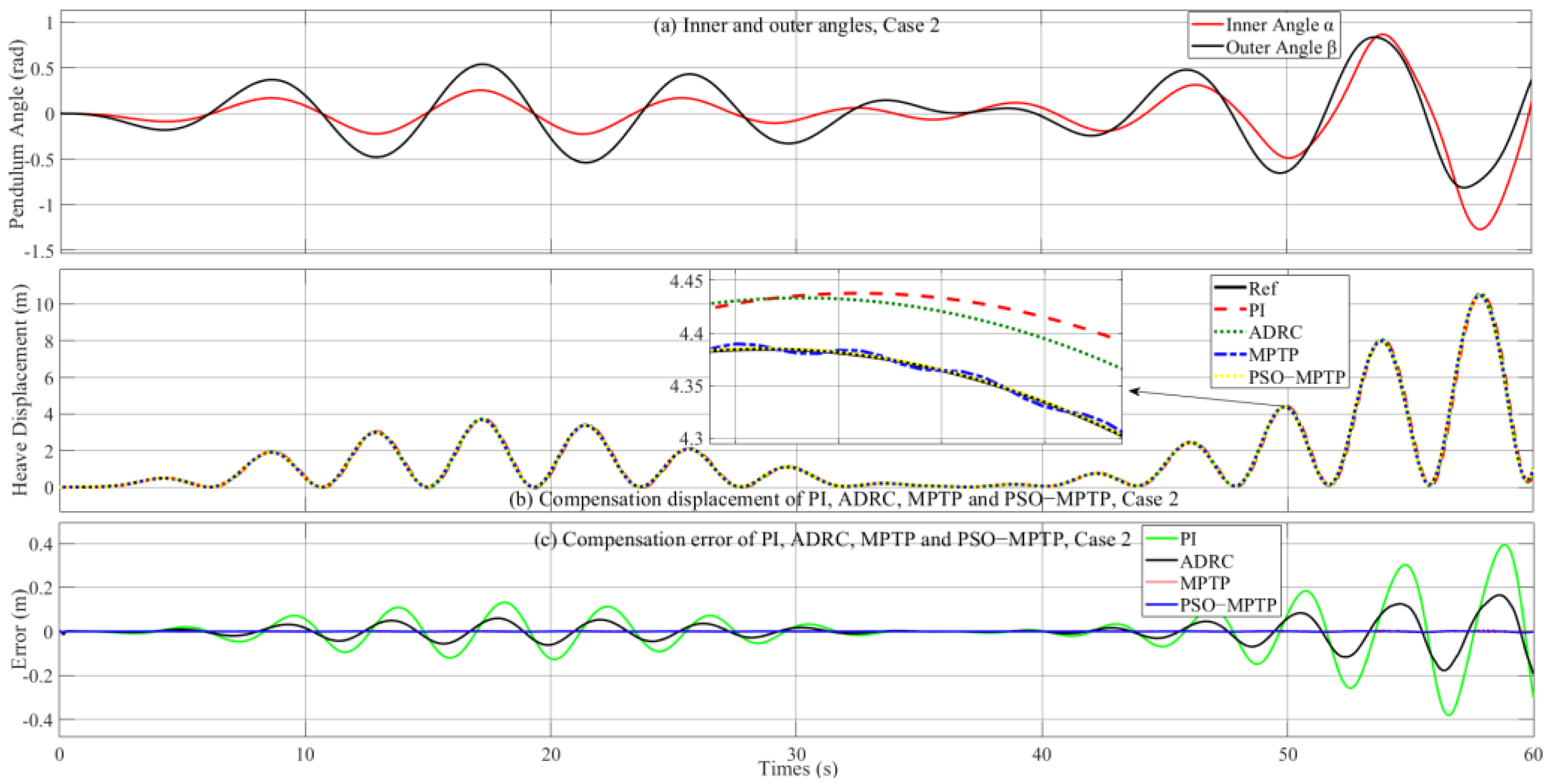
Case 2: L = 25 m and V = 0.2 m/s

In this case, the crane load decreases at a constant speed of V = 0.2 m/s. In Figure 10, the inner and outer angles are larger and larger, and the shaking is more serious. The swing amplitude of the inner and the outer angles are bigger than that in case 1, and the heave displacement of the crane load is significantly increased in this working condition. It can be seen from Figure 10 that the maximum displacement of the crane load in the heave direction is approximately 10.5 m. The CE of PI is 94.3%, the CE of ADRC is 95.3%, the CE of MPTP is 99%, and the CE of PSO−MPTP is 99.8%.

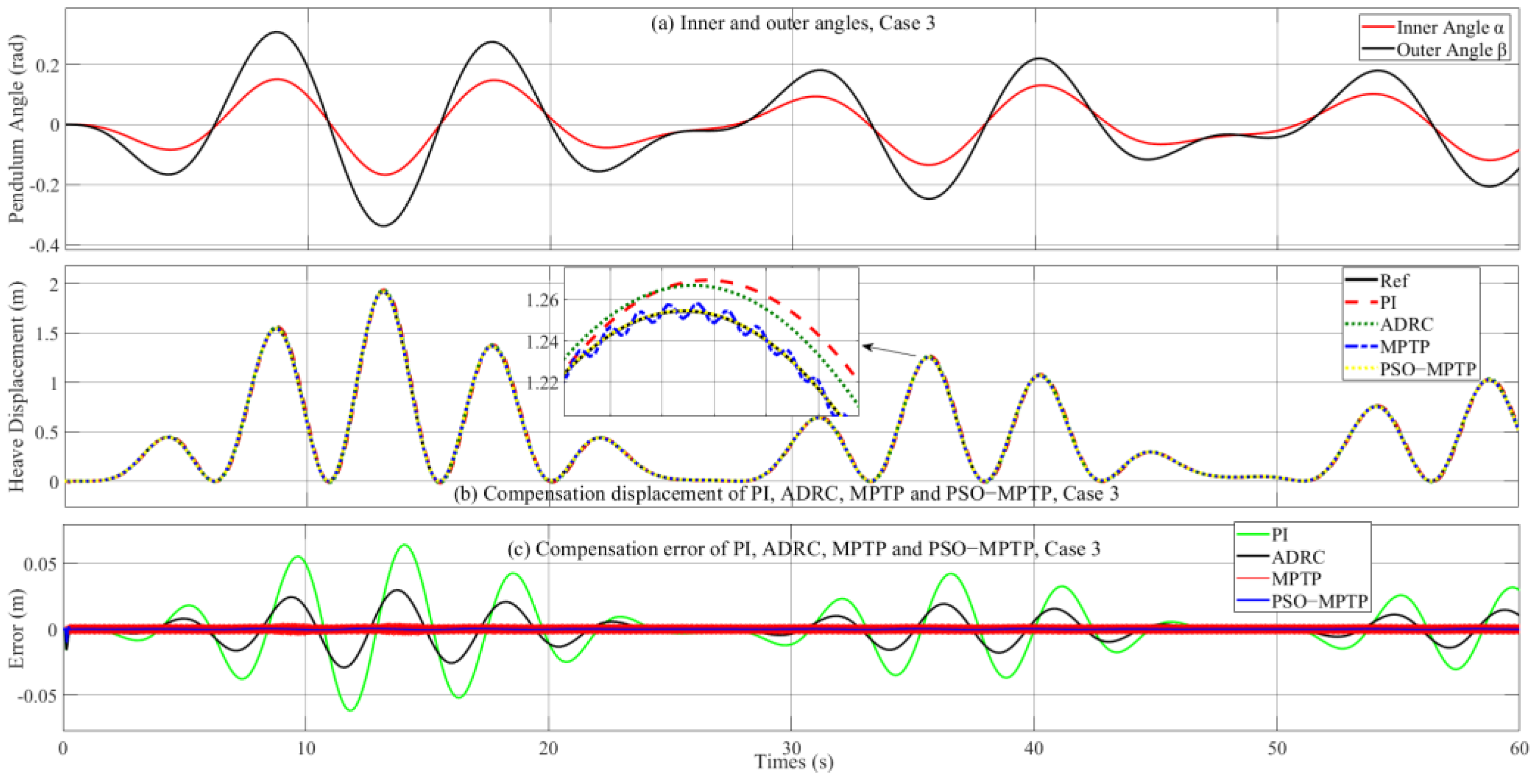
Case 3: L = 25 m and V = −0.2 m/s

In this case, the crane load increases at a constant speed of V = −0.2 m/s. From Figure 11, the inner and outer angles are smaller than that in the other two cases and the maximum displacement in the heave direction is bigger, up to approximately 1.8 m. The CE of PI is 95.4%, the CE of ADRC is 98.1%, the CE of MPTP is 99.2%, and the CE of PSO−MPTP is 99.9%; the heave displacement is significantly reduced.

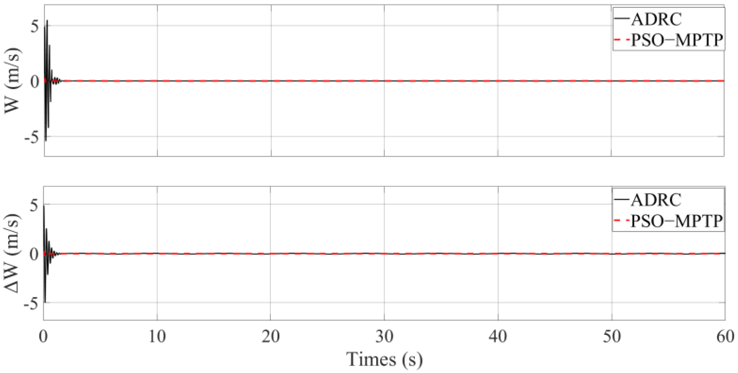
In order to test ΔW and W of PSO−MPTP and ADRC, the most severe working conditions, Case 2, are selected for testing. The simulation results are shown in Figure 12. According to this figure, ΔW and W of ADRC exceed the constraint, while ΔW and W of PSO−MPTP are within the constraint, ensuring the smooth operation of machinery and equipment and personal safety.

In this section, three different working conditions are introduced when the crane is working. Under the same impact of sea waves, CE of PSO−MPTP is better than that of ADRC, and the control effect is relatively smooth and stable in all three cases. Whether lifting or lowering the crane load, the compensation system can compensate well in poor sea conditions.

5.2. Robustness Analysis

5.2.1. White Noise

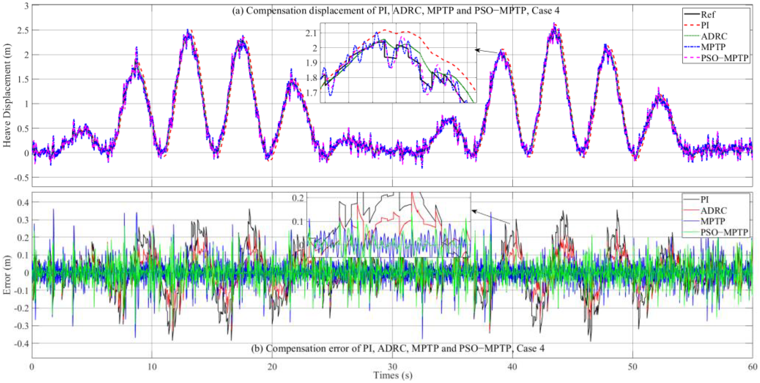
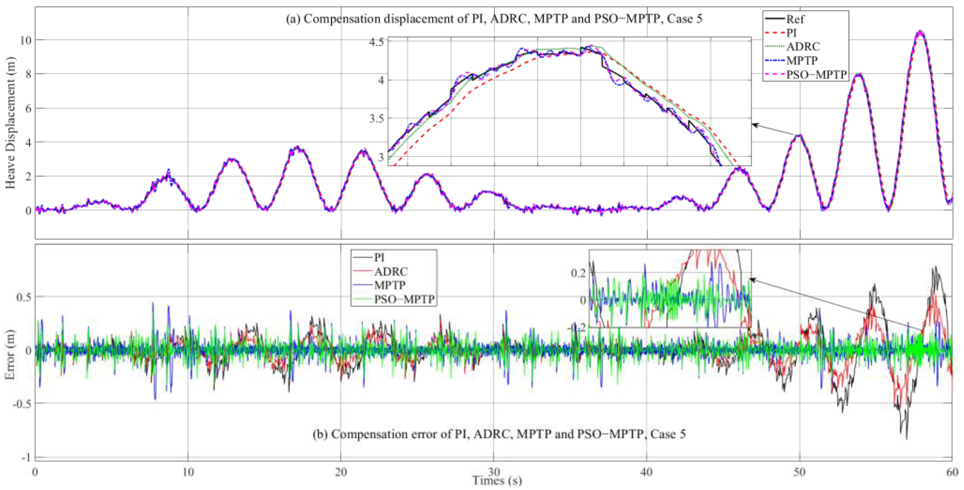
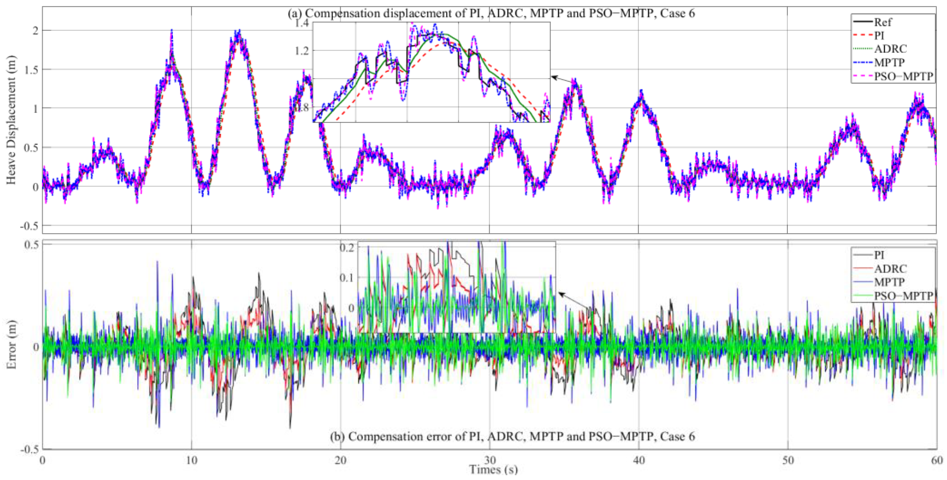
In actual work, unexpected disturbance is inevitable. The compensation system and ship would be interfered with by the harsh environment. In order to analyze the anti-interference ability of PSO−MPTP, white noise is used as the actual noise interference, and white noise and ΔZ superposition are used as the input signal of the position loop. In this section, three cases, as in the previous part, are simulated for the analysis (Case 4: With noise, L = 25 m, V = 0 m/s; Case 5: With noise, L = 25 m, V = 0.2 m/s; Case 6: With noise, L = 25 m, V = −0.2 m/s).

From Figure 13, Figure 14 and Figure 15, even the noise is added to the system, PSO−MPTP always presents better performances than that of ADRC. For these three cases, CEs of PSO−MPTP are 94.1%, 94.8%, and 94.2%, respectively; CEs of MPTP are 93.3%, 92.9%, and 93%, respectively; CEs of ADRC are 91.3%, 91.9%, and 91%; CEs of PI are 85.3%, 85.9%, and 87%, respectively. Although these values are relatively smaller than that in the ideal conditions, the compensation effect is still excellent and can be accepted.

5.2.2. Parameter Variation

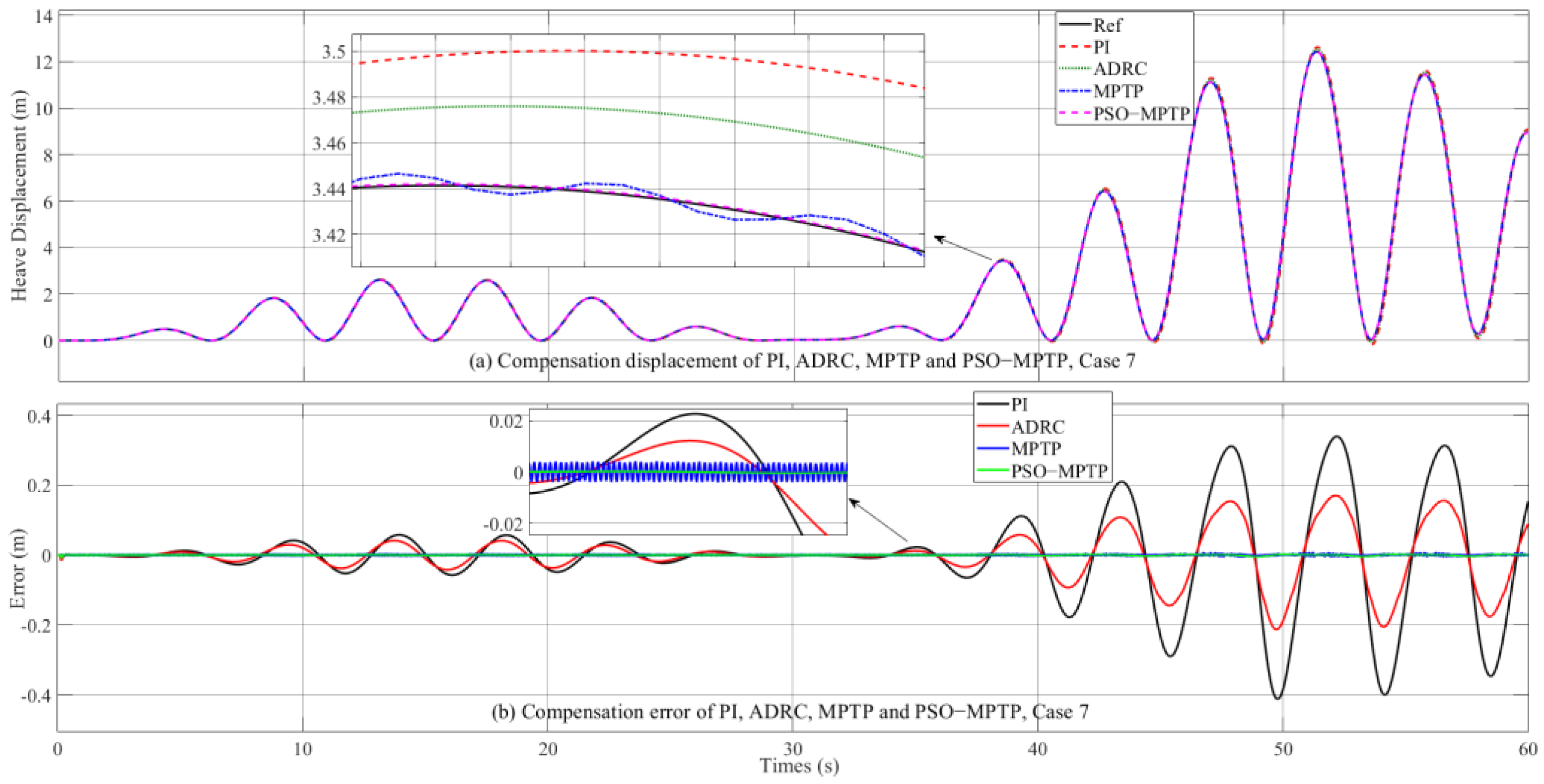
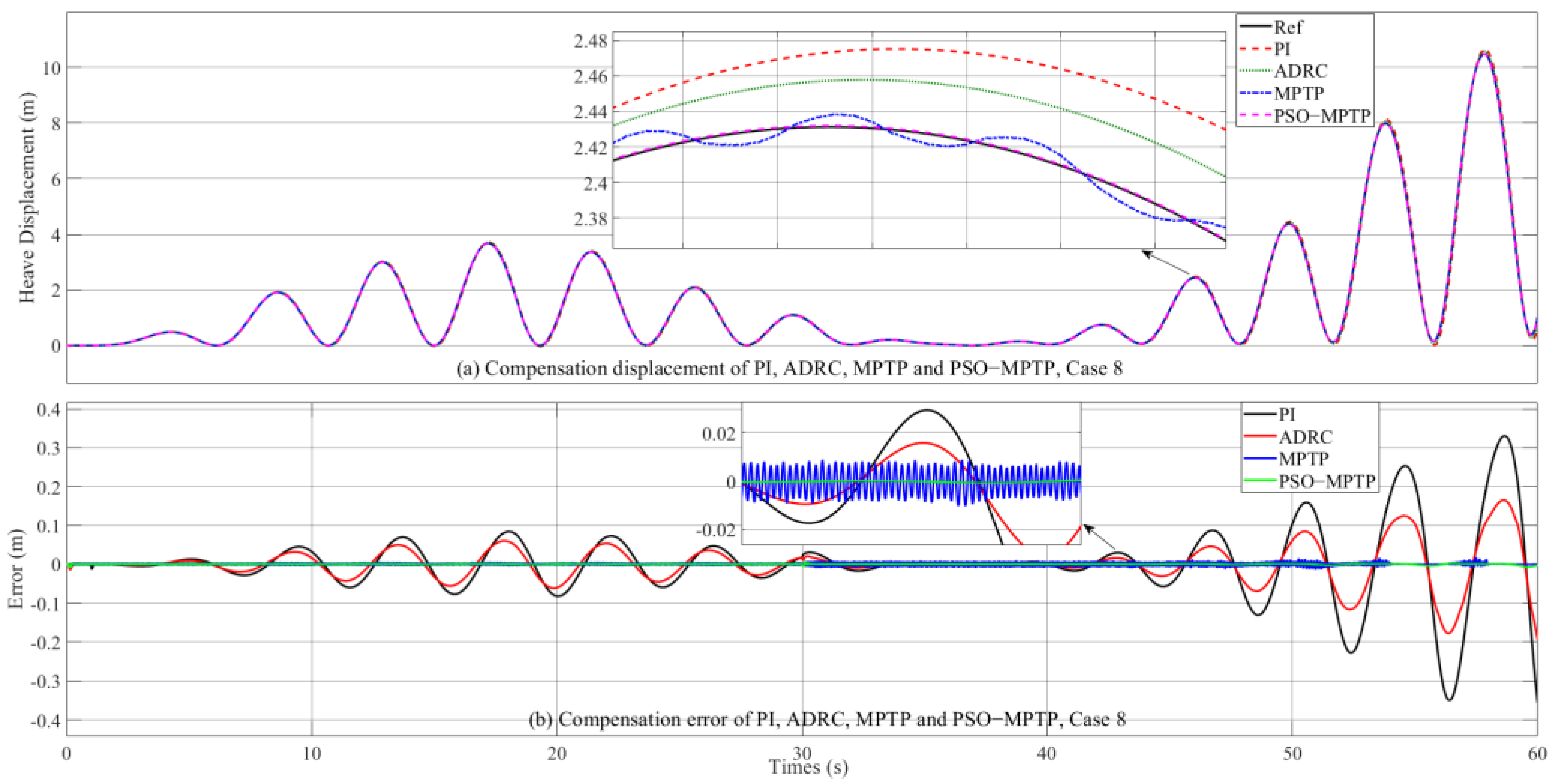
In actual work, system parameters may change due to the working conditions. For example, the wave encounter angle may change when the hull encounters a wave, and the parameters of PMSM may also be verified due to the high humidity and salt fog. Therefore, in this section, the working condition L = 25 m, V = 0.2 m/s and a level 4 sea state are selected to analyze these two problems (Case 7: L = 25 m, V = 0.2 m/s, wave encounter angle changes; Case 8: L = 25 m, V = 0.2 m/s, parameters of PMSM change).

For Case 7, the wave encounter angle φ changes from π/4 to π/3 and impacts the hull at t = 30 s. As shown in Figure 16, when the angle φ changes, the heave displacement greatly increases and ca reach approximately 12.5 m. After the compensation under this condition, the CE of PSO−MPTP is still as high as 99.7% with only a 0.1% reduction compared with Case 2. The CE of MPTP is 98.3%, while for ADRC and PI, CEs are reduced by nearly 1–5% and equal to 94.1% and 89%.

For Case 8, to verify the robustness of the PSO−MPTP, the PMSM parameters also change at t = 30 s, R_s changes from 4 Ω to 5 Ω, and L_d and L_q change from 0.07 mH to 0.08 mH. As shown in Figure 17, the track performance of PI becomes worse after t = 30 s, while the track performance of PSO−MPTP is still excellent. Although the compensation errors of PSO−MPTP and MPTP are slightly worse than that in Case 2, the CEs of PSO−MPTP and MPTP are still as high as 99.7% and 98.8%, respectively, while for ADRC and PI, CEs are only 94.3% and 90.1%, respectively.

6. Conclusions

This paper firstly introduced the principle of heave compensation and modeled the wave disturbance force and the ship crane system. Second, the displacement of the crane load in the heave direction was obtained through the Lagrangian equation and the differential equation of the system. Then, the PSO−MPTP was established through the motion state equation of the crane load and firstly added to the position loop. PSO was used to solve the quadratic programming in MPTP, which further improves CE and the operation speed of MPTP. PSO−MPTP provides a solid foundation for future hardware experiments. The system uses the multi-step predicted position signal of the crane load, which finishes the three-phase closed-loop of the PMSM. Finally, the compensation problem of crane load heave and displacement under the action of waves under three different working conditions was analyzed. The results show that displacement compensation can be performed well under different working conditions with a CE of more than 99%. Robustness analysis was also carried out in this paper. In the simulation, whether the system is disturbed by white noise or motor parameter variations, the CE of PSO−MPTP far exceeds the CEs of PI and ADRC and can reach more than 94%.

It can be seen that PSO−MPTP has strong robustness to disturbances for nonlinear systems and relatively smooth control effects compared to PI and ADRC. Whether lifting or lowering the crane load, the compensation system can compensate well in poor sea conditions, which guarantees the safety of the crane load and personnel to a great extent. However, as this paper only considers the heave displacement of the crane load and ignores the wind disturbance to the sling, it simplifies the system model and makes the PSO−MPTP compensation efficient. Subsequent research needs to decouple and compensate for the sway of the crane load in other directions and the wind disturbance.