
Synchronized Motion-Based UAV–USV Cooperative Autonomous Landing

1
The School of Electrical Engineering, Anhui Polytechnic University, Wuhu 241000, China
2
The School of Artificial Intelligence and Automation, Huazhong University of Science and Technology, Wuhan 430074, China
3
The Suzhou USTAR Intelligent Technology Co., Ltd., Suzhou 215000, China
*
Author to whom correspondence should be addressed.
J. Mar. Sci. Eng. 2022, 10(9), 1214; https://doi.org/10.3390/jmse10091214
Submission received: 27 July 2022
/
Revised: 25 August 2022
/
Accepted: 28 August 2022
/
Published: 31 August 2022
(This article belongs to the Section Ocean Engineering)
Abstract
:A synchronous motion-based control strategy for unmanned aerial vehicle (UAV) landing on an unmanned surface vehicle (USV) is proposed to address the problem of low accuracy or even failure of UAV landing on the surface of a USV under wave action. Firstly, the landing marks are identified and localized based on computer vision; secondly, the USV attitude angle is predicted based on a bidirectional long-short term memory (Bi-LSTM) neural network to ensure that the UAV can respond to USV attitude changes in real-time; furthermore, the UAV attitude controller is designed based on a PID algorithm to realize UAV–USV synchronous motion. The experimental results demonstrate that the proposed UAV–USV synchronous motion landing scheme with high landing accuracy is more suitable for the UAV to achieve autonomous landing on a USV in a complex marine environment.
1. Introduction
In the recent years, with the gradual application of the unmanned system on the maritime battlefield, the form of maritime warfare has further developed towards unmanned combat. As a new type of weapon system in future maritime war, the technological development of maritime unmanned systems is of great significance to the maintenance of national maritime rights and interests [1]. In coastal warfare, an unmanned surface vehicle (USV) can realize maritime patrols and recharge an unmanned aerial vehicle (UAV). With the ability of realizing reconnaissance and surveillance of the sky and the beach, a UAV can complement the advantages of a UAV and USV, thus forming a cooperative combat system [2,3].
One of the most important aspects of the UAV–USV cooperative warfare system is the ability of the UAV to land accurately on the USV with changing attitude. However, due to the impact of the harsh marine environment, as well as the enemy setting up radio signal interference in the course of combat and other challenges, it is difficult for the UAV to achieve autonomous landing on a USV. To this end, this paper proposes a UAV–USV cooperative autonomous landing control strategy based on synchronous motion. The main contributions of this paper are summarized as follows:
- (1)
- The UAV–USV cooperative autonomous landing method based on synchronous motion is proposed to improve the landing accuracy of a UAV in the harsh marine environment.
- (2)
- Aiming at the problem that UAV–USV cannot be synchronized in real-time during the landing process, a USV attitude prediction algorithm based on a bidirectional long-short-term memory (Bi-LSTM) neural network is proposed.
- (3)
- In order to realize UAV–USV synchronous motion, the UAV pose controller is designed based on the proportional-integral-derivative (PID) algorithm.
The rest of this paper is organized as follows. Section 2 briefly discusses the related work. The mathematical model of the UAV–USV synchronous motion landing system is given in Section 3. The design principles of the Bi-LSTM neural network-based predictive controller and the PID algorithm-based attitude controller are given in Section 4. Section 5 verifies the effectiveness and superiority of the UAV–USV synchronous motion landing strategy proposed in this paper in terms of landing accuracy through simulation experiments. Finally, Section 6 summarizes the conclusions.
2. Related Works
In this section, we present a brief literature review in order to offer an overview of research work on aspects related to UAV landing. This review is not meant to be complete, and it only aims to show how our method differentiates from previous work.
Until now, the autonomous landing of a UAV remains one of the most challenging tasks. In the process of UAV landing, the precise landing cannot be achieved if only the global positioning system (GPS) is used for positioning. Landing accuracy can be improved by combining multi-sensor data fusion techniques, including data fusion of radar altimeter (RALT) with GPS [4,5], GPS with inertial navigation system (INS) [6], and ultra-wideband beacons with inertial measurement units [7]. Whereas, the multi-sensor data fusion method will generate sensor noise, and the installation of additional sensors will exceed the UAV load, thus reducing flexibility. Therefore, it is important to study an efficient and low-cost UAV landing strategy for UAV–USV cooperative operations.
With the development of computer vision technology, the vision-based localization method has been widely used in UAV landing. Due to the uncertainty of the motion platform, existing studies are based mostly on fixed platform landing. Patruno et al. [8] proposed a vision-based UAV landing auxiliary algorithm, which can ensure that the UAV accurately identifies the target and lands autonomously in the cluttered environment. Lin et al. [9] designed a new vision system to help a UAV land autonomously in light-limited environments. However, due to the renewed complexity and variability of maritime combat missions, the landing method of the fixed platform can no longer meet the mission requirements. Thus, recent research was diverted to the autonomous landing of a UAV on the moving platform. Zhao et al. [10] proposed a robust visual servo control method to solve the time delay problem of the UAV landing on the moving platform. Kwak et al. [11] designed a landing platform with leveling function combined with computer vision, the platform can enable the UAV to land smoothly even if the landing platform is located on steep terrain. Gautam et al. [12] developed a logarithmic polynomial closed-loop speed controller, which enables UAVs to land on the motion platform more accurately. Niu et al. [13] proposed an autonomous landing system based on vision, which allows under the condition of no GPS signal UAV to land autonomously on moving unmanned ground vehicle (UGV). Persson et al. [14] proposed a model predictive control algorithm to solve the problem of cooperative rendezvous between UAV and UGV, with whose control strategy, the UAV can also land safely on a mobile UGV under wind disturbance.
However, compared with mobile platforms on land, USVs are subject to wave interference in the marine environment, which poses a greater challenge for autonomous UAV landings. Polvara et al. [15,16,17], by installing landing markers on the USV deck and combining them with deep reinforcement learning, analyzed the landing markers to improve the accuracy of UAV attitude estimation and further improve the accuracy of UAV landing. Bochan et al. [18] developed an automatic UAV landing system that combines machine vision and a nonlinear controller, where the UAV can remotely identify the landing point and successfully land on a moving USV. Lapandic et al. [19] proposed a cooperative UAV–USV landing control scheme based on distributed model predictive control, which can update UAV–USV rendezvous information in real-time to ensure that UAV–USV will arrive at the rendezvous point synchronously and land successfully. Ross et al. [20] designed a marine condition predictor to compensate for ship motion, which makes UAV landing on a USV more smoothly.
However, under the influence of sea waves, sea winds, and bad weather, the USV attitude will change at any time. In the final stage of UAV landing, a UAV only relies on visual guidance to land [16,17,18] or controls the USV to land in a relatively static situation [15,20]. In these methods, the UAV does not respond to the attitude change of the USV, and it cannot always ensure that the UAV can accurately land on the USV. In this paper, a UAV–USV cooperative autonomous landing control strategy based on synchronous motion is proposed, which can make the UAV consistent with the attitude of the USV in the final landing process, improve the landing accuracy of the UAV, and make the UAV realize the landing operation smoothly and safely.
3. System Modeling
In this section, the mathematical model of UAV–USV synchronous motion and the pose calculation principle based on the ar_pose visual library [21] are introduced.
3.1. Establishment of UAV–USV Synchronous Movement Coordinate System
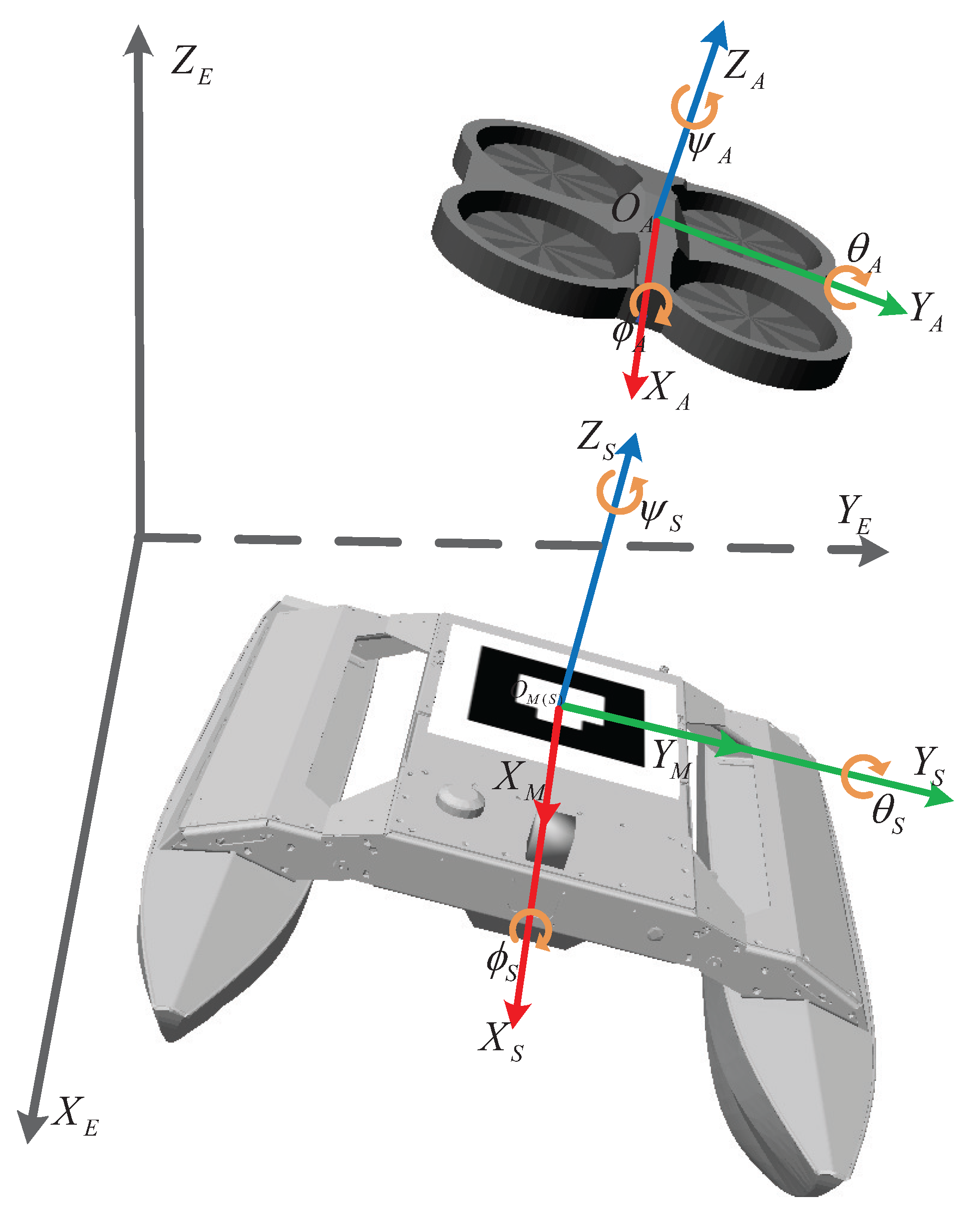
The UAV–USV synchronous motion coordinate system (shown in Figure 1) is established [22], including the earth coordinate system, the carrier coordinate system, and the landing mark coordinate system. is the earth coordinate system, defined by the East-North-Up (ENU). The carrier coordinate system includes the UAV coordinate system and the USV coordinate system , which is defined by the Front-Left-Up (FLU). is the landing mark coordinate system.
In the actual analysis, the carrier coordinate system needs to be converted to the earth coordinate system for analysis. The conversion matrix is:
where subscript B represents the carrier coordinate system. and represent and , respectively.
3.2. Modeling of UAV
In this paper, the AR Drone 2.0 quadrotor UAV is used as the research object [23,24]. As shown in Figure 1, represents the position of the UAV in the earth coordinate system; is the cross-roll angle, pitch angle, and yaw angle, respectively, which indicate the direction of the UAV in the earth coordinate system. Without considering the wind disturbance and other environmental disturbance factors, the UAV is mainly subjected to thrust for its gravity, air resistance, and four rotor blades. The force analysis of the UAV is:
where, is the mass of UAV, T is the thrust in the direction of the -axis, represent the air resistance in the direction of , respectively. The mathematical model of the UAV is as follows:
where represent ; is the angular velocity in the carrier system.
3.3. Modeling of USV
This paper mainly studies the pitching and rolling motions of the USV caused by ocean currents, as shown in Figure 1, which represents the position of the USV in the earth coordinate system, and also represents the azimuth of the USV in the earth coordinate system. The USV kinematic model is established as follows [25]:
where and represent the linear velocity and angular velocity, respectively, and represent .
3.4. Pose Calculation
In this paper, the ar_pose computer vision library is used to calculate the pose. During the UAV landing process, the UAV down-looking camera is used to search for the landing mark. After obtaining the pixel coordinates of the landing mark , the pose calculation is converted to the coordinates in the earth coordinate system (assuming that the landing platform height is zero). The pose calculation relationship is:
where are the central coordinates of the image, are the parameters of the camera, and the obtained coordinate is the reference value of the UAV position, and represent .
4. Proposed Method
The overall framework of the method for precise UAV landing on a USV based on synchronized motion (as shown in Figure 2) is composed of three parts: computer vision-based positioning is used to ensure that the UAV is always located directly above the landing mark center during the UAV landing process; a Bi-LSTM neural network is used to predict the USV attitude angle to ensure that UAVs respond to USV attitude changes in real-time. The UAV is controlled based on the PID algorithm, which makes the UAV and USV keep in synchronous movement for an accurate landing.
4.1. Predictive Controller
This section introduces the basic principles of long-short-term memory (LSTM) neural network and bidirectional long-short-term memory (Bi-LSTM) neural network, and use Bi-LSTM to predict the change of the USV attitude angle.
4.1.1. LSTM Neural Network
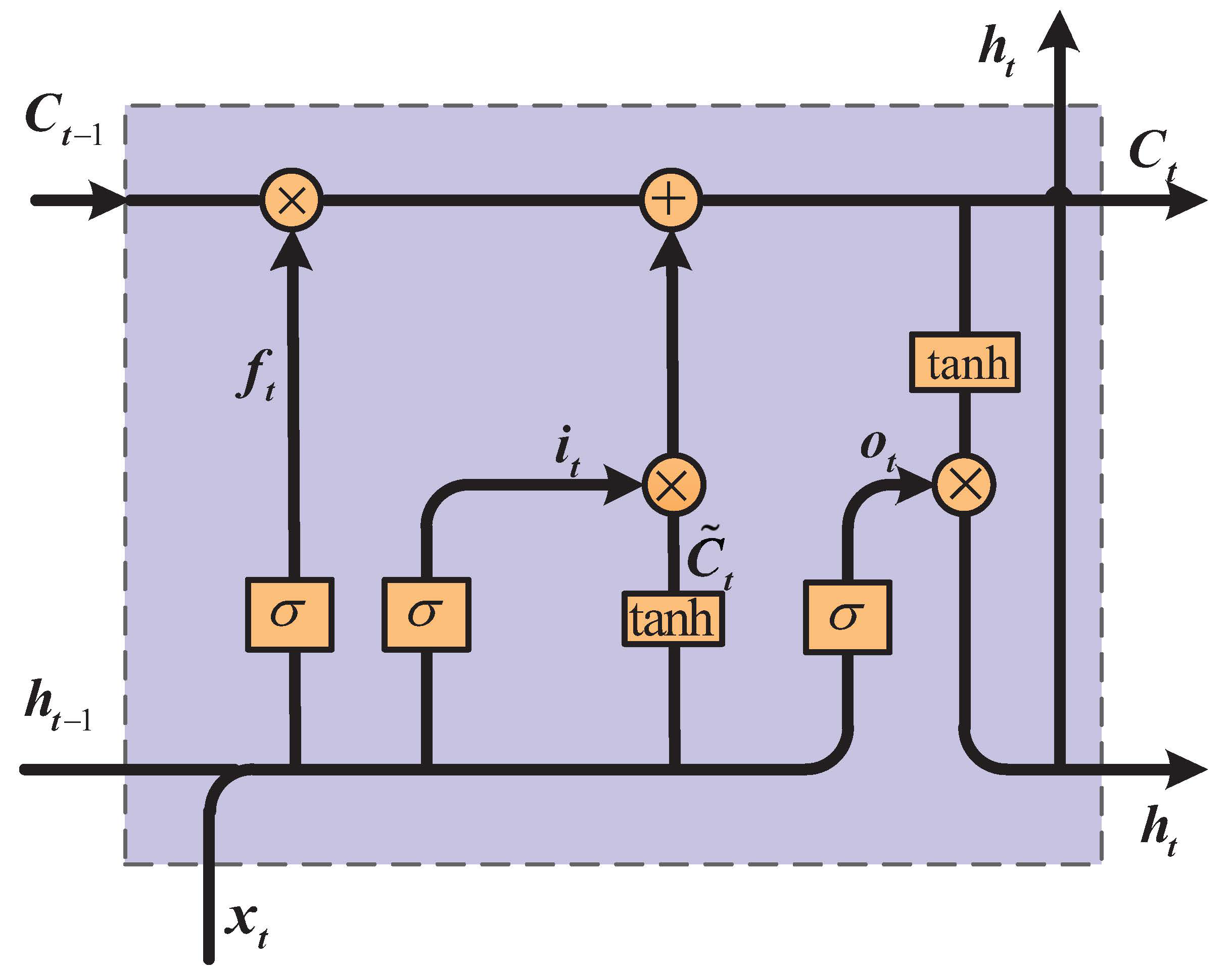
In USV motion, there is a strong correlation between attitude angle change and time series. Based on the historical data on the USV motion attitude, the time series analysis method can better predict the future attitude change. As a special kind of recurrent neural network (RNN), the LSTM neural network solves the problem of gradient disappearance and gradient explosion of RNN in the long-term sequence training process. It can better remember the time series data and is more suitable for predicting the ship’s attitude [26,27]. The unit structure of LSTM is shown in Figure 3. The LSTM neural network is characterized by the fact that it contains input gates, forgetting gates, and output gates. These gates are used to update and discard historical information so that LSTM can perform long-term memory. The principal formula of the LSTM neural network is as follows:
where denote the input gate, the forgetting gate, and the output gate; represent the input layer parameters at the current time, the hidden layer state at the previous time, and the temporary state; and represent the weight matrix and bias of each door, respectively. and are sigmoid functions and hyperbolic tangent functions, respectively. According to the results of Equations (6)–(9), the current state and output are:
where ⊙ is the element-wise product.
4.1.2. Bi-LSTM Neural Network
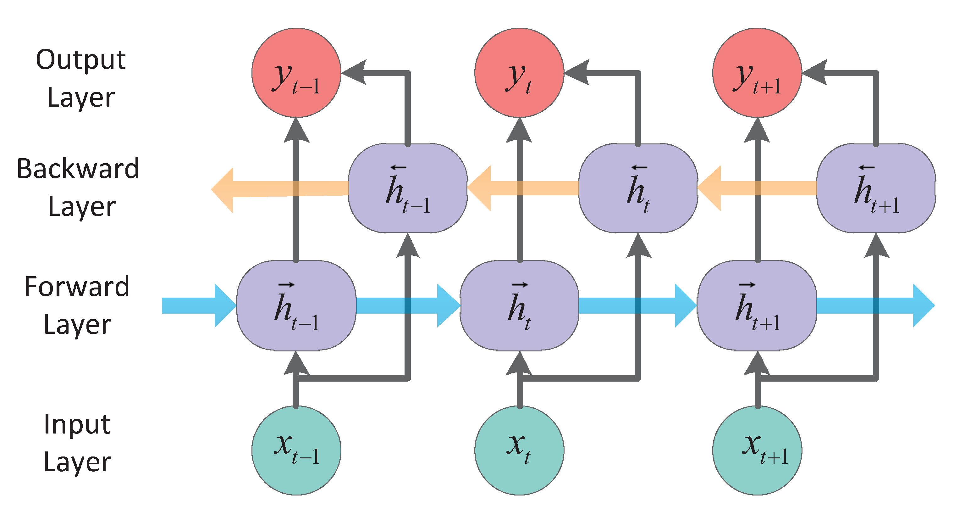
LSTM neural network only considers the influence of a past state on the current state when predicting a time series. The network ignores the influence of a future state on the current state, which cannot satisfy the accurate prediction of the USV posture. The Bi-directional long and short-term memory (Bi-LSTM) neural network [28] is further developed on the basis of LSTM, which consists of a forward LSTM neural network and reversed LSTM neural network. The past and future state information can be used to do the prediction, which can better reflect the trend of the time series, and provides a more accurate prediction of the ship’s motion attitude [29,30]. The Bi-LSTM neural network structure is shown in Figure 4.
Combining the hidden layer states obtained in different directions yields the output layer result at time t which is:
4.2. Pose Controller
In order to better control UAV–USV to keep synchronous motion, this paper designs a UAV pose controller based on the PID control algorithm [31,32]. The state of the UAV is . In the process of UAV–USV synchronous movement landing, the expected position is . It is necessary to control the UAV to land near the landing sign center and keep it synchronized with the attitude of the USV.
From the mathematical model of the UAV, it can be seen that the quadrotor UAV has four control inputs of , and six degrees of freedom for . The number of its degrees of freedom is much larger than the number of control inputs, so the quadrotor UAV is a typical underactuated control system. For the underactuated quadrotor UAV, its position cannot be driven directly and needs to be driven indirectly by . Therefore, the coupling relationship between different states needs to be used reasonably when designing the controller. Based on this, the PID controller designed in this paper is described as follows:
where represent the four control signals of the controller; represent the desired attitude, which combines the predicted USV attitude angle with the position control value . are the virtual control signals, which represent the position of the indirect control UAV in the direction. () denote the gain parameters of proportional, integral and differential of PID controller. The specific design is as follows:
In this paper, based on the experience of engineering applications, experiments are conducted directly in the simulation system to adjust the gain parameters of the PID controller. Firstly, all gain parameters are initialized to zero, and the integral and differential links are removed, so that the UAV system becomes a pure proportional adjustment method. Increasing the value until the UAV begins to oscillate slightly; secondly, followed by a small increase in to suppress UAV oscillations until the UAV reaches stability; finally, the value is continuously increased to improve the response speed of the UAV under the premise of system stability. Simulation experiments are used to continuously adjust the size of the parameters of each link, so that the UAV can respond to the control signal quickly and stably. The gain parameters of the PID controller selected for the simulation experiments in this paper are shown in Table 1.
4.3. UAV–USV Synchronous Motion Landing Algorithm
The principle of UAV–USV synchronous motion landing method is shown in Algorithm 1. In this paper, we focus on the landing stage of UAV in the UAV–USV collaborative control process. First, the landing mark is required to be always within the field of vision of the UAV down-looking camera during the UAV landing. When the UAV height is less than the altitude threshold (set to 2–3 m), the UAV takes the predicted USV attitude angle as a reference signal and responds to the USV attitude change in real-time to keep the UAV and the USV in synchronous motion. At the same time, the UAV is controlled to reduce the offset with the landing mark center in the direction to ensure that the UAV can land at the center of the landing point. When the UAV offset in the direction is less than the set threshold and the UAV height is less than the height threshold (set to 0.15–0.25 m), the current vertical velocity of the UAV is increased to , and the UAV will accelerate to land on the USV to complete the autonomous landing task. By this method, the autonomous landing operation of the UAV can be achieved even if the USV is affected by the wave-current and produces pitch roll motion.
| Algorithm 1 UAV–USV Synchronous Motion Landing Algorithm |
|
5. Simulation Results
In order to verify the effectiveness and superiority of the synchronous motion-based UAV landing method proposed in this paper, simulation comparison experiments were conducted. All experiments were conducted under the Ubuntu 14.04.6 system. The simulation simulator used ROS-indigo and Gazebo-2.2.6 platforms [33]. The UAV simulation platform included an AR Drone quadrotor UAV and tum_simulator simulation control package. The USV used Kingfisher_USV provided by ROS as the landing platform. In this paper, the landing logo is identified and located based on the ar_pose visual library. The 4 × 4_8 tag in the ar_pose visual library is designed as the landing logo. To ensure that the unmanned boat is not tilted by waves during the cyclic motion, the maximum wave variation simulated is set not to exceed ten degrees [34].
In this paper, several simulation experiments are conducted under different conditions. The experiment consists of three parts. In the first part, the Bi-LSTM neural network is used to predict the attitude angle change of the USV; the second part introduces the landing situation of the UAV under the condition of USV pitching motion, conducts multiple landing experiments of UAV–USV synchronous movement and UAV–USV conventional movement, respectively, and compares and analyzes the final experimental results. UAV–USV conventional motion means that the UAV does not respond to USV attitude change, and the landing process is vertical landing. The UAV–USV conventional motion landing method can be found in the literature [16]. The third part introduces the landing situation of a UAV under the condition of USV roll motion, and the experimental process is the same as that of the second part.
5.1. USV Attitude Prediction
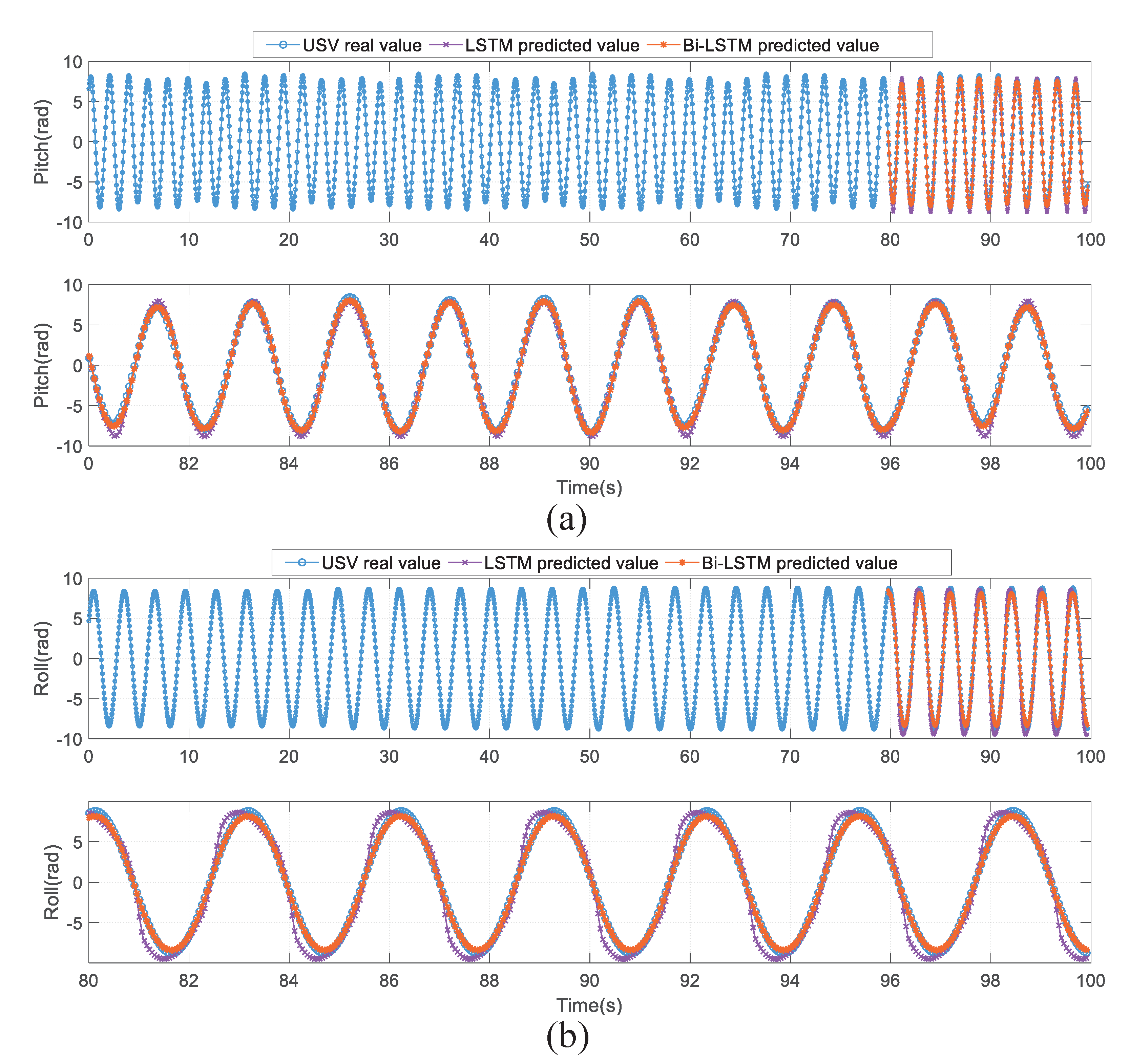
In the marine environment, the effects of USV pitch and roll motions on UAV landing on a USV are more obvious and needs to be focused on. In this paper, the attitude data of pitch motion and roll motion generated by the USV running in the simulation system for 100 s are selected, and the LSTM neural network model and Bi-LSTM neural network model are used for training and prediction, respectively. The prediction results are shown in Figure 5.
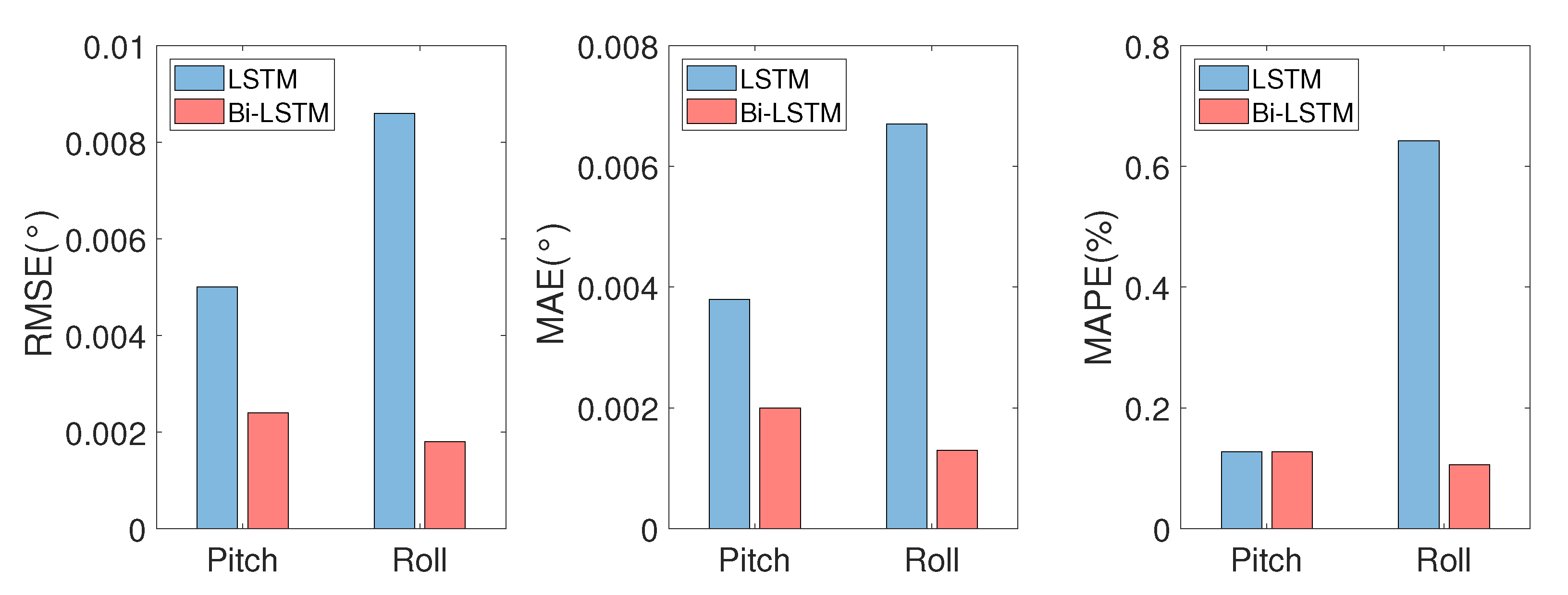
As shown in Figure 5, the ratio of the training set to the test set is 8:2, i.e., the first 80 s are the training data and the second 20 s are test data. The difference between the predicted results and the actual USV values is shown in the diagram. In order to better compare the accuracy of the prediction results, the following evaluation indexes are introduced: Root Mean Square Error (RMSE), Mean Absolute Errors (MAE), and Mean Absolute Percentage Errors (MAPE). The results of the comparative analysis of prediction errors are shown in Table 2 and Figure 6.
The smaller the error evaluation index is, the better the prediction results are. From the results of Table 2 and Figure 6, the Bi-LSTM neural network prediction model is compared with LSTM neural network prediction model. The former is used in the pitch angle prediction results, where evaluation index RMSE, MAE, MAPE decreased , , , respectively; in terms of the roll angle prediction results, the evaluation indexes RMSE, MAE, MAPE decrease , , , respectively. The results of the evaluation indexes show that the prediction results of the Bi-LSTM neural network model are more accurate and can better fit the actual attitude value of USV, which is more suitable for the UAV–USV synchronous motion landing control method in this paper.
5.2. USV Pitching Motion
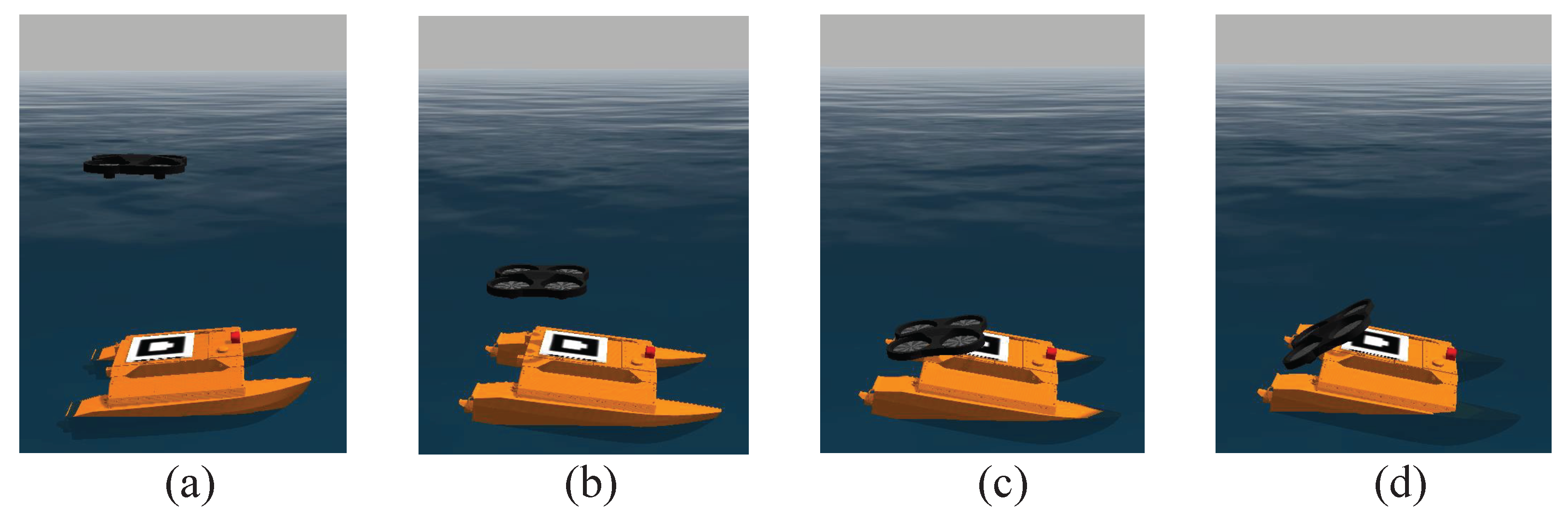
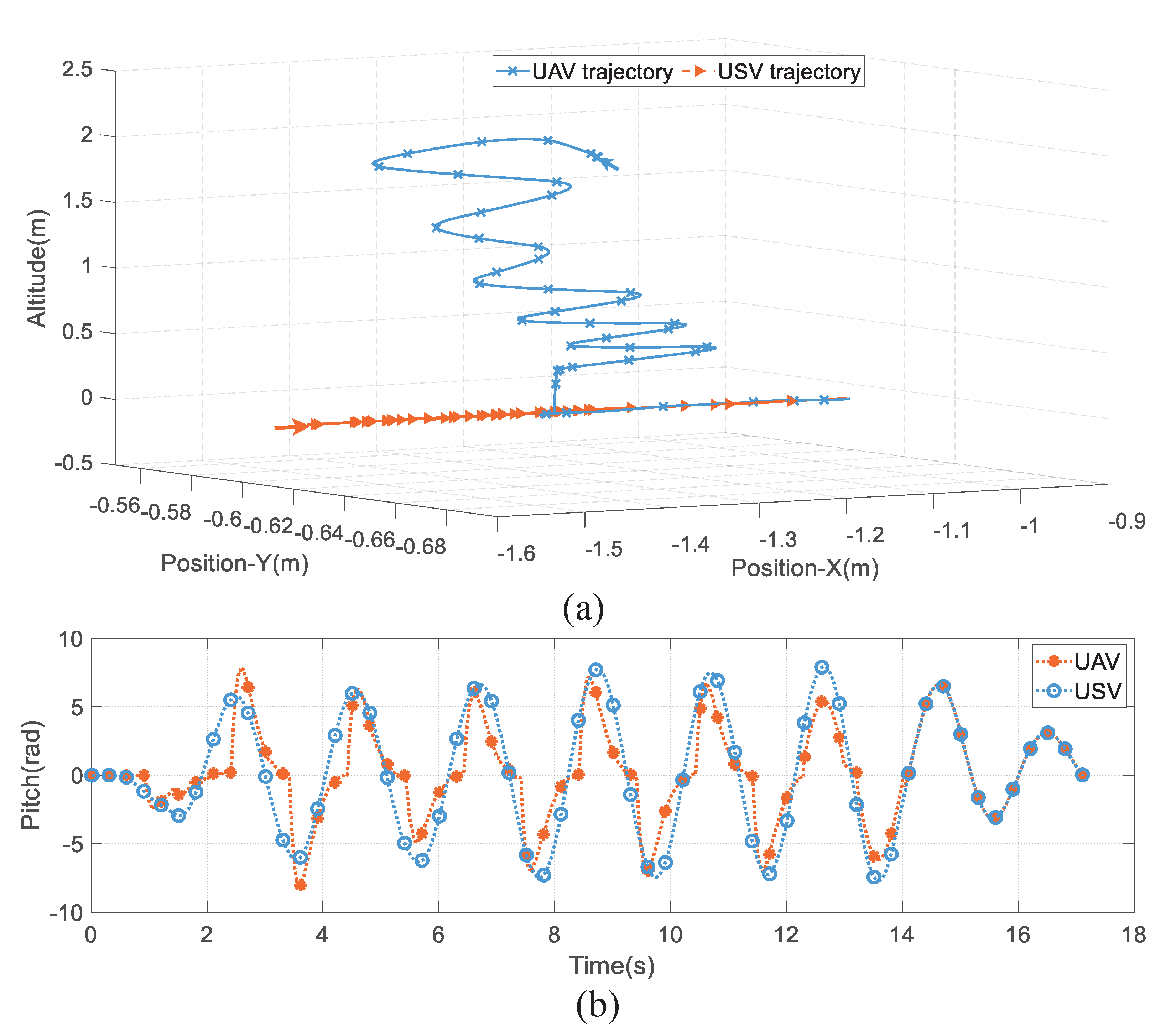
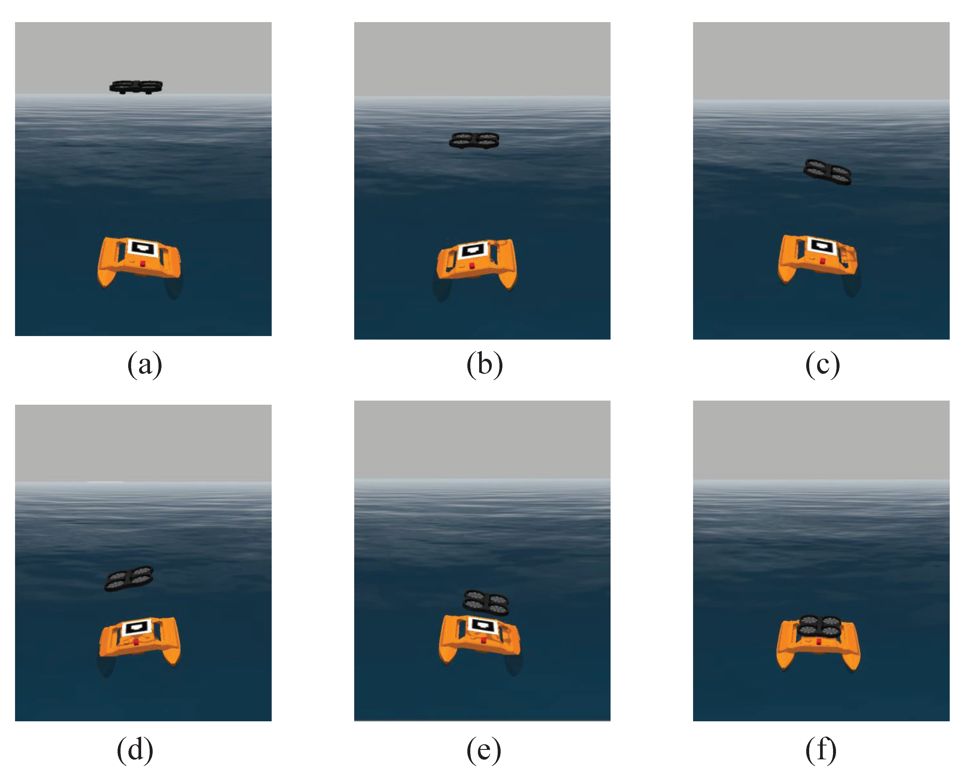
This section analyzes the landing situation of a UAV under the pitch motion condition under the influence of waves. In this scenario, the pitching motion of the USV is greater than the rolling motion, and the USV moves mainly along the direction. Ten UAV–USV synchronous motion landing experiments and ten UAV–USV conventional motion landing experiments [16] were conducted separately, and the landing accuracy was analyzed in comparison. Figure 7 shows the failure situation of UAV landing under the condition of USV pitching motion using the UAV–USV conventional motion landing method. Figure 8 reflects the three-dimensional trajectories of the UAV and USV, and the variation of UAV-USV pitch angle. Figure 9 reflects the variation of the UAV landing position under USV pitching motion. Figure 10 shows the important moments in the simulation of USV pitching motion. Figure 11 analyzes the landing accuracy of UAV–USV synchronous movement and conventional movement under the condition of USV pitching motion.
As shown in Figure 7, the UAV landed using the UAV–USV conventional motion landing method under the USV pitch motion condition. The UAV did not respond to the attitude change of the USV, and the landing process was a vertical landing (Figure 7a–c). When the USV pitch angle changed greatly, the UAV collided with the stern of the USV, resulting in the failure of the UAV landing (Figure 7c,d).
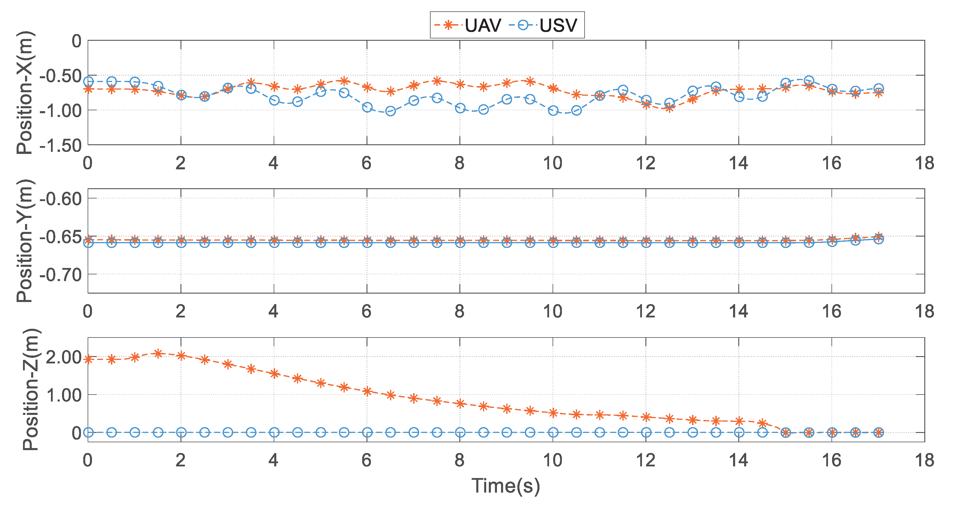
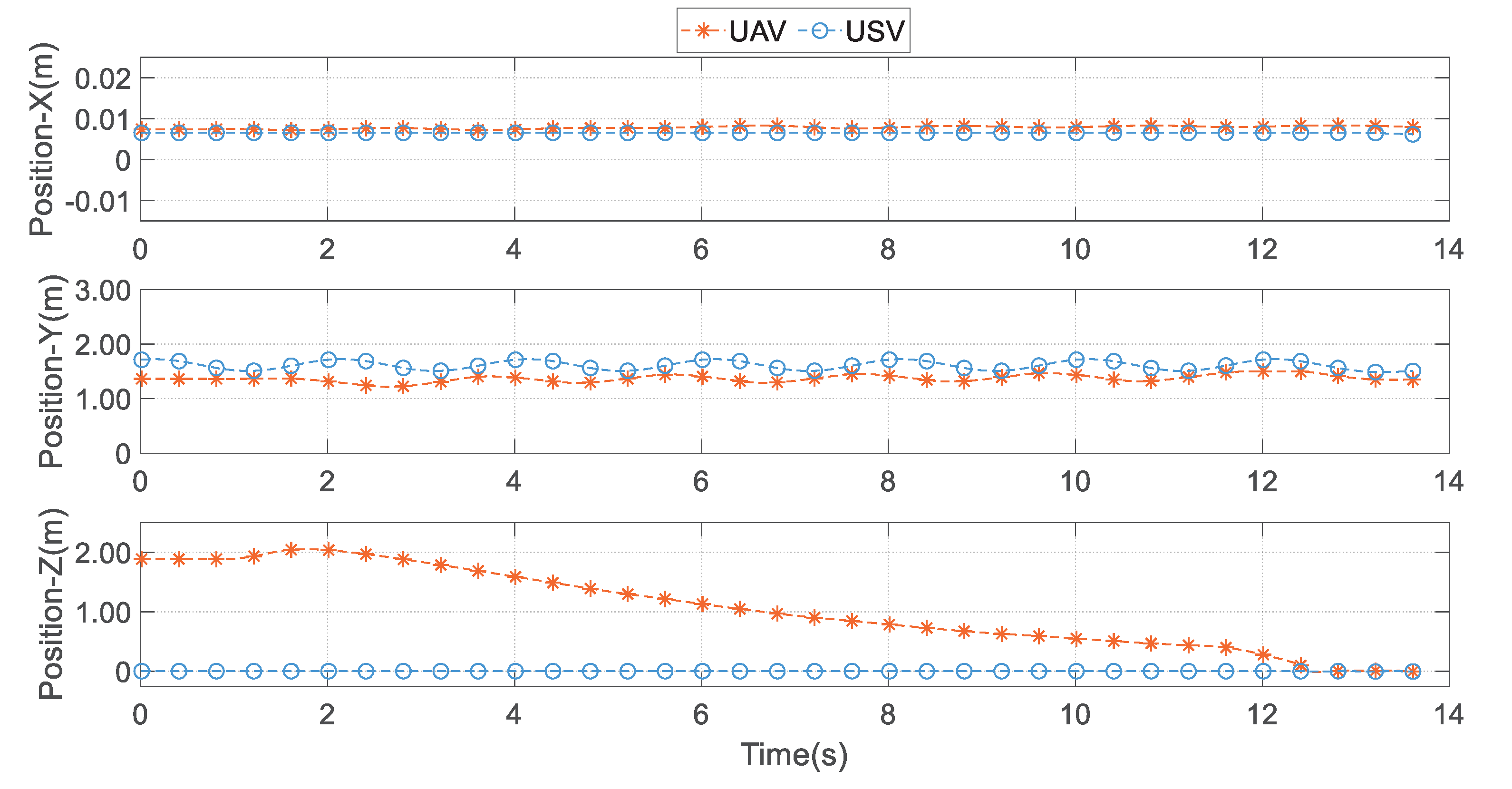
As seen in Figure 8, Figure 9 and Figure 10, the UAV can land in pitch motion within 14 s. The UAV remains in hover until the landing command is received. When the landing instruction is sent at time s, the UAV rises to a certain altitude to adjust its attitude, and the landing sign is located in the field of vision. At time s, when the UAV height is less than the height threshold , it enters the first stage of landing. The UAV takes the predicted USV elevation angle as the reference signal, keeps real-time synchronization with USV, and reduces its height. When the UAV moves to s, the current UAV height is 0.35 m, and it will land on the USV at this time. Therefore, the variation of the pitch angle is reduced accordingly, which is prepared for the smooth landing on the USV. At time s, when the UAV enters the second stage of landing, the UAV height is less than the height threshold , the UAV offset in the direction is within the threshold range, and the UAV accelerates to land on the USV deck to complete the landing operation. The landing errors of the UAV final landing point and USV deck center in the direction are m and m, respectively. The two-dimensional Euclidean distance between the UAV’s final landing point and the USV deck center is m. As shown in Figure 9, the USV pitching motion will produce the position change in the direction, and the UAV and the USV attitude remain synchronized, so the UAV position will also change accordingly. At this time, the USV does not occur in roll motion, so the position of the UAV in the direction remains relatively static, which is conducive to the accurate landing of the UAV.
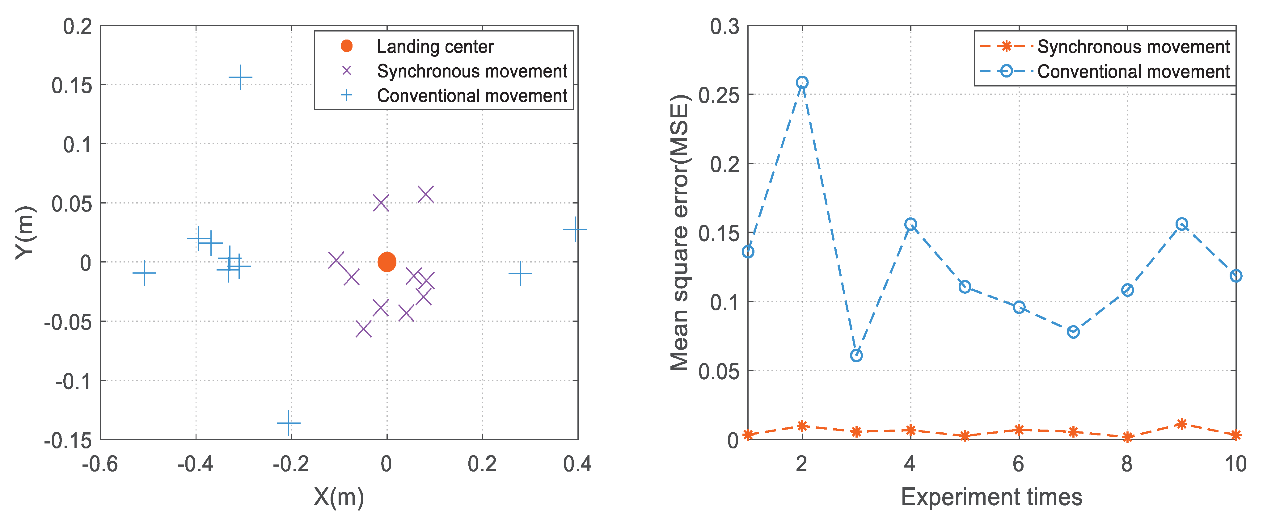
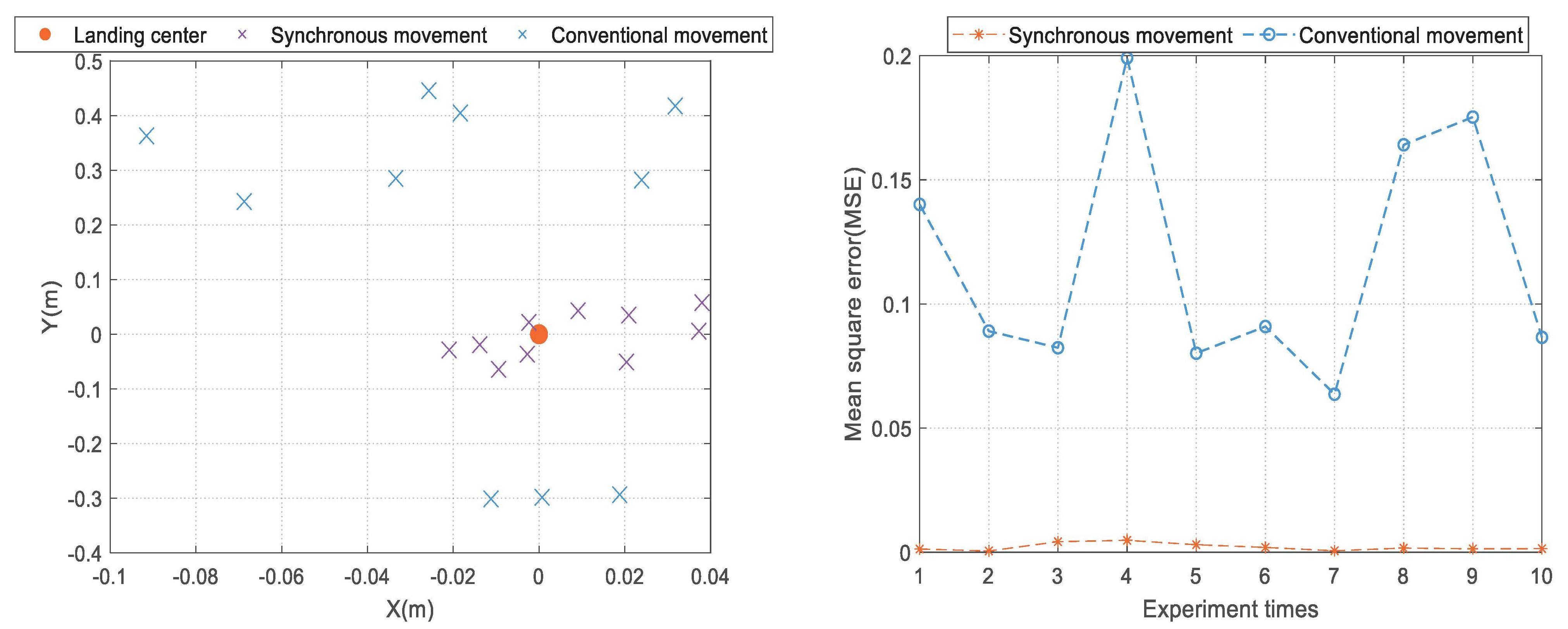
The landing accuracy of different control strategies can be obtained by calculating the two-dimensional Euclidean distance between the final landing point of the UAV and the center point of the USV deck. As shown in Figure 11 (left), the UAV–USV synchronous motion landing point is located in range 0.2 m × 0.12 m and the UAV–USV conventional motion landing point is located in range 0.9 m × 0.3 m. To facilitate the analysis, the mean square error (MSE) is introduced to determine the error from the landing center point. As shown in Figure 11 (right), the mean MSE of UAV–USV synchronous movement landing is 0.0731, and the mean MSE of UAV–USV conventional movement landing is 0.3509. According to the analysis results, in the case of USV pitching motion, the UAV–USV synchronous movement landing method proposed in this paper can achieve more accurate autonomous landing of the UAV.
5.3. USV Roll Motion
This section analyzes the landing situation of UAV under the roll motion condition under the influence of waves. In this scenario, the rolling motion of the USV is greater than the pitching motion, and the USV moves mainly in the direction. We perform the same number of experiments under USV pitching motion. Figure 12 shows the failure situation of UAV landing under the condition of USV roll motion using UAV–USV conventional motion landing method. Figure 13 reflects the 3D trajectories of the UAV and USV, and the variation of UAV–USV roll angle. Figure 14 reflects the variation of the UAV landing position under USV roll motion. Figure 15 shows the important moments in the simulation of USV roll motion. Figure 16 analyzes the landing accuracy of UAV–USV synchronous movement and conventional movement under the condition of USV roll motion.
As shown in Figure 12, the UAV landed using the UAV–USV conventional motion landing method under the USV roll motion condition. The UAV did not respond to the attitude change of the USV, and the landing process was a vertical landing (Figure 12a–c). When the USV roll angle changed greatly, the UAV collided with the side of the USV, resulting in the failure of the UAV landing (Figure 12c,d).
It can be seen from Figure 13, Figure 14 and Figure 15 that under the condition of USV roll motion, the UAV can complete the autonomous landing within 12 s. At time s, the UAV receives the landing command, and the UAV angle is used to adjust the field of vision. At time s, the UAV height is less than the height threshold . The UAV uses the predicted USV roll angle as the reference signal, and the UAV–USV maintains synchronous movement while reducing the UAV height. When s, the UAV height is less than the height threshold , and the UAV is located above the landing point center, then the UAV accelerates to land on the USV deck to complete the autonomous landing. The landing errors of the UAV final landing point and USV deck center in the direction are m and m, respectively. The two-dimensional Euclidean distance between the UAV’s final landing point and the USV deck center is m. As shown in Figure 14, the USV roll motion will produce the position change in the direction, and the UAV and the USV attitude remain synchronized, so the UAV position will also change accordingly. At this time, the USV does not occur in pitch motion, so the position of the UAV in the direction remains relatively static, which is conducive to the accurate landing of the UAV.
The analysis of the landing accuracy under USV roll motion and pitching motion is consistent. As shown in Figure 16 (left), the UAV–USV synchronous motion landing point is located in range 0.06 m × 0.13 m and the UAV–USV conventional motion landing point is located in range 0.12 m × 0.75 m. As shown in Figure 16 (right), the mean MSE of UAV–USV synchronous movement landing is 0.0429, and the mean MSE of UAV–USV conventional movement landing is 0.3361. The analysis results show that the landing accuracy of the UAV–USV synchronous motion landing method has higher landing accuracy under USV transverse rocking conditions and is more suitable for autonomous UAV landing in a complex marine environment.
6. Conclusions and Future Directions
In this paper, a UAV–USV synchronous motion control method for UAV autonomous landing is studied. The USV attitude prediction controller is designed by a Bi-LSTM neural network, and the UAV pose controller is designed by a PID algorithm to guarantee the real-time synchronization movement of the UAV–USV.
In order to verify the advancedness of the proposed method, several sets of comparison experiments were conducted between the proposed method and the UAV–USV conventional motion landing method. UAV–USV conventional motion means that the the UAV does not respond to a USV attitude change, and the landing process is vertical landing. Simulation results show that compared with the UAV–USV conventional movement landing method, the UAV–USV synchronous movement landing method can effectively improve the landing accuracy, which is more suitable for the UAV to realize autonomous and accurate landing in a harsh marine environment.
This paper mainly proposes an autonomous UAV landing control strategy without further optimization of the controller. Future research should focus on developing and optimizing the controller and comparing it with other control methods (e.g., robust control or nonlinear control). Due to the complexity of the scenario in which the USV pitch motion is coupled with the roll motion, the landing of the UAV in this scenario is not discussed in this paper, which is an essential consideration for future research. In this paper, we focus on the influence of wave motion on the landing process of the UAV, without further considering the more complex marine environment such as the sea breeze, which is an important aspect of future research.
Author Contributions
Conceptualization, W.L. and Y.G.; methodology, W.L. and Y.G.; software, W.L. and Y.G.; validation, W.L., Y.G., Z.G. and G.Y.; formal analysis, W.L., Y.G., Z.G. and G.Y.; investigation, W.L., Y.G., Z.G. and G.Y.; resources, W.L., Y.G., Z.G. and G.Y.; data curation, W.L., Y.G., Z.G. and G.Y.; writing—original draft preparation, W.L., Y.G., Z.G. and G.Y.; writing—review and editing, W.L., Y.G., Z.G. and G.Y.; visualization, W.L., Y.G., Z.G. and G.Y.; supervision, W.L., Y.G., Z.G. and G.Y.; project administration, W.L., Y.G., Z.G. and G.Y.; funding acquisition, W.L., Y.G., Z.G. and G.Y. All authors have read and agreed to the published version of the manuscript.
Funding
This work is supported partially by National Natural Science Foundation of China (NSFC) (No. U21A20146, No. 61976099). This work was supported by the Open Foundation Project of State Key Laboratory of Power System and Generation Equipment (No. SKLD21KM09), the Synergy Innovation Program of Anhui Polytechnic University and Jiujiang District (No. 2021cyxta2), and Wuhu Science and Technology Project (No. 2021cg19).
Institutional Review Board Statement
Not applicable.
Informed Consent Statement
Not applicable.
Data Availability Statement
The data that support the findings of this study are available from the corresponding author upon reasonable request.
Conflicts of Interest
The authors declare no conflict of interest.
References
- Xie, W.; Tao, H.; Gong, J.; Luo, W.; Yin, F.; Liang, X. Research advances in the development status and key technology of unmanned marine vehicle swarm operation. Chin. J. Ship Res. 2021, 16, 7–17. [Google Scholar]
- Zhang, H.; He, Y.; Li, D.; Gu, F.; Li, Q.; Zhang, M.; Di, C.; Chu, L.; Chen, B.; Hu, Y. Marine UAV–USV marsupial platform: System and recovery technic verification. Appl. Sci. 2020, 10, 1583. [Google Scholar] [CrossRef]
- Shao, G.; Ma, Y.; Malekian, R.; Yan, X.; Li, Z. A novel cooperative platform design for coupled USV–UAV systems. IEEE Trans. Ind. Inform. 2019, 15, 4913–4922. [Google Scholar] [CrossRef]
- Abujoub, S.; Mcphee, J.; Westin, C.; Irani, R.A. Unmanned aerial vehicle landing on maritime vessels using signal prediction of the ship motion. In Proceedings of the OCEANS 2018 MTS/IEEE Charleston, Charleston, SC, USA, 22–25 October 2018; pp. 1–9. [Google Scholar]
- Videmsek, A.; de Haag, M.U.; Bleakley, T. Sensitivity analysis of RADAR Altimeter-aided GPS for UAS precision approach. In Proceedings of the 32nd International Technical Meeting of the Satellite Division of The Institute of Navigation (ION GNSS+ 2019), Miami, FL, USA, 16–20 September 2019; pp. 2521–2538. [Google Scholar]
- Li, W.; Fu, Z. Unmanned aerial vehicle positioning based on multi-sensor information fusion. Geo-Spat. Inf. Sci. 2018, 21, 302–310. [Google Scholar] [CrossRef]
- Meng, Y.; Wang, W.; Han, H.; Ban, J. A visual/inertial integrated landing guidance method for UAV landing on the ship. Aerosp. Sci. Technol. 2019, 85, 474–480. [Google Scholar] [CrossRef]
- Patruno, C.; Nitti, M.; Petitti, A.; Stella, E.; D’Orazio, T. A vision-based approach for unmanned aerial vehicle landing. J. Intell. Robot. Syst. 2019, 95, 645–664. [Google Scholar] [CrossRef]
- Lin, S.; Jin, L.; Chen, Z. Real-Time Monocular Vision System for UAV Autonomous Landing in Outdoor Low-Illumination Environments. Sensors 2021, 21, 6226. [Google Scholar] [CrossRef] [PubMed]
- Zhao, W.; Liu, H.; Wang, X. Robust visual servoing control for quadrotors landing on a moving target. J. Frankl. Inst. 2021, 358, 2301–2319. [Google Scholar] [CrossRef]
- Kwak, J.; Lee, S.; Baek, J.; Chu, B. Autonomous UAV Target Tracking and Safe Landing on a Leveling Mobile Platform. Int. J. Precis. Eng. Manuf. 2022, 23, 305–317. [Google Scholar] [CrossRef]
- Gautam, A.; Singh, M.; Sujit, P.B.; Saripalli, S. Autonomous Quadcopter Landing on a Moving Target. Sensors 2022, 22, 1116. [Google Scholar] [CrossRef]
- Niu, G.; Yang, Q.; Gao, Y.; Pun, M.O. Vision-based Autonomous Landing for Unmanned Aerial and Mobile Ground Vehicles Cooperative Systems. IEEE Robot. Autom. Lett. 2022, 7, 6234–6241. [Google Scholar] [CrossRef]
- Persson, L.; Muskardin, T.; Wahlberg, B. Cooperative rendezvous of ground vehicle and aerial vehicle using model predictive control. In Proceedings of the 2017 IEEE 56th Annual Conference on Decision and Control (CDC), Melbourne, VIC, Australia, 12–15 December 2017; pp. 2819–2824. [Google Scholar]
- Polvara, R.; Sharma, S.; Wan, J.; Manning, A.; Sutton, R. Towards autonomous landing on a moving vessel through fiducial markers. In Proceedings of the 2017 European Conference on Mobile Robots (ECMR), Paris, France, 6–8 September 2017; pp. 1–6. [Google Scholar]
- Polvara, R.; Sharma, S.; Wan, J.; Manning, A.; Sutton, R. Vision-based autonomous landing of a quadrotor on the perturbed deck of an unmanned surface vehicle. Drones 2018, 2, 15. [Google Scholar] [CrossRef]
- Polvara, R.; Sharma, S.; Wan, J.; Manning, A.; Sutton, R. Autonomous vehicular landings on the deck of an unmanned surface vehicle using deep reinforcement learning. Robotica 2019, 37, 1867–1882. [Google Scholar] [CrossRef]
- Lee, B.; Saj, V.; Benedict, M.; Kalathil, D. Intelligent Vision-based Autonomous Ship Landing of VTOL UAVs. arXiv 2022, arXiv:2202.13005. [Google Scholar]
- Lapandić, D.; Persson, L.; Dimarogonas, D.V.; Wahlberg, B. Aperiodic Communication for MPC in Autonomous Cooperative Landing. IFAC-PapersOnLine 2021, 54, 113–118. [Google Scholar] [CrossRef]
- Ross, J.; Seto, M.; Johnston, C. Autonomous Landing of Rotary Wing Unmanned Aerial Vehicles on Underway Ships in a Sea State. J. Intell. Robot. Syst. 2022, 104, 1–9. [Google Scholar] [CrossRef]
- Ivan, D.; Bill, M.; Gautier, D. Ar_pose. Available online: http://wiki.ros.org/ar_pose (accessed on 16 April 2022).
- Wang, N.; Ahn, C.K. Coordinated Trajectory-Tracking Control of a Marine Aerial-Surface Heterogeneous System. IEEE/ASME Trans. Mechatronics 2021, 26, 3198–3210. [Google Scholar] [CrossRef]
- Engel, J.; Sturm, J.; Cremers, D. Camera-based navigation of a low-cost quadrocopter. In Proceedings of the 2012 IEEE/RSJ International Conference on Intelligent Robots and Systems, Vilamoura-Algarve, Portugal, 7–12 October 2012; pp. 2815–2821. [Google Scholar]
- Engel, J.; Sturm, J.; Cremers, D. Scale-aware navigation of a low-cost quadrocopter with a monocular camera. Robot. Auton. Syst. 2014, 62, 1646–1656. [Google Scholar] [CrossRef]
- McCue, L. Handbook of marine craft hydrodynamics and motion control [bookshelf]. IEEE Control. Syst. Mag. 2016, 36, 78–79. [Google Scholar]
- Zhang, T.; Zheng, X.Q.; Liu, M.X. Multiscale attention-based LSTM for ship motion prediction. Ocean. Eng. 2021, 230, 109066. [Google Scholar] [CrossRef]
- Hu, X.; Zhang, B.; Tang, G. Research on ship motion prediction algorithm based on dual-pass Long Short-Term Memory neural network. IEEE Access 2021, 9, 28429–28438. [Google Scholar] [CrossRef]
- Hochreiter, S.; Schmidhuber, J. Long short-term memory. Neural Comput. 1997, 9, 1735–1780. [Google Scholar] [CrossRef] [PubMed]
- Wang, Y.; Wang, H.; Zou, D.; Fu, H. Ship roll prediction algorithm based on Bi-LSTM-TPA combined model. J. Mar. Sci. Eng. 2021, 9, 387. [Google Scholar] [CrossRef]
- Park, J.; Jeong, J.; Park, Y. Ship trajectory prediction based on bi-LSTM using spectral-clustered AIS data. J. Mar. Sci. Eng. 2021, 9, 1037. [Google Scholar] [CrossRef]
- Rohr, D.; Stastny, T.; Verling, S.; Siegwart, R. Attitude and cruise control of a VTOL tiltwing UAV. IEEE Robot. Autom. Lett. 2019, 4, 2683–2690. [Google Scholar] [CrossRef] [Green Version]
- Babu, V.M.; Das, K.; Kumar, S. Designing of self tuning PID controller for AR drone quadrotor. In Proceedings of the 2017 18th international conference on advanced robotics (ICAR), Hong Kong, China, 10–12 July 2017; pp. 167–172. [Google Scholar]
- Quigley, M.; Gerkey, B.P.; Conley, K.; Faust, J.; Ng, A.Y. ROS: An open-source Robot Operating System. In Proceedings of the ICRA Workshop on Open Source Software, Kobe, Japan, 12–17 May 2009. [Google Scholar]
- McAdams, T. Slope Limits; Aircraft Owners and Pilots Association: Frederick, MD, USA, 2012. [Google Scholar]
Figure 1.
UAV–USV synchronous movement coordinate system. is the earth coordinate system, defined by East−North−Up (ENU). The carrier coordinate system includes the UAV coordinate system and the USV coordinate system , which is defined by Front−Left−Up (FLU). is the landing mark coordinate system.
Figure 1.
UAV–USV synchronous movement coordinate system. is the earth coordinate system, defined by East−North−Up (ENU). The carrier coordinate system includes the UAV coordinate system and the USV coordinate system , which is defined by Front−Left−Up (FLU). is the landing mark coordinate system.

Figure 2.
The overall framework of the method for precise UAV landing on a USV based on synchronized motion. Computer vision−based positioning to ensure that the UAV is always located directly above the landing mark center during the UAV landing process; a Bi-LSTM neural network is used to predict the USV attitude angle to ensure that UAVs respond to USV attitude changes in real−time; the UAV is controlled based on the PID algorithm, which makes the UAV and USV keep in synchronous movement for an accurate landing.

Figure 3.
LSTM neural network structure.

Figure 4.
Bi-LSTM neural network structure.

Figure 5.
(a) pitch angle prediction results of USV; (b) roll angle prediction results of USV. The ratio of the training set to the test set is 8:2, i.e., the first 80 s are the training data and the second 20 s are test data.
Figure 5.
(a) pitch angle prediction results of USV; (b) roll angle prediction results of USV. The ratio of the training set to the test set is 8:2, i.e., the first 80 s are the training data and the second 20 s are test data.

Figure 6.
Error statistical histogram of USV attitude angle prediction.

Figure 7.
USV pitching motion−failure situation of UAV landing.The UAV did not respond to the attitude change of the USV, and the landing process was a vertical landing (a–c). When the USV pitch angle changed greatly, the UAV collided with the stern of the USV, resulting in the failure of the UAV landing (c,d).

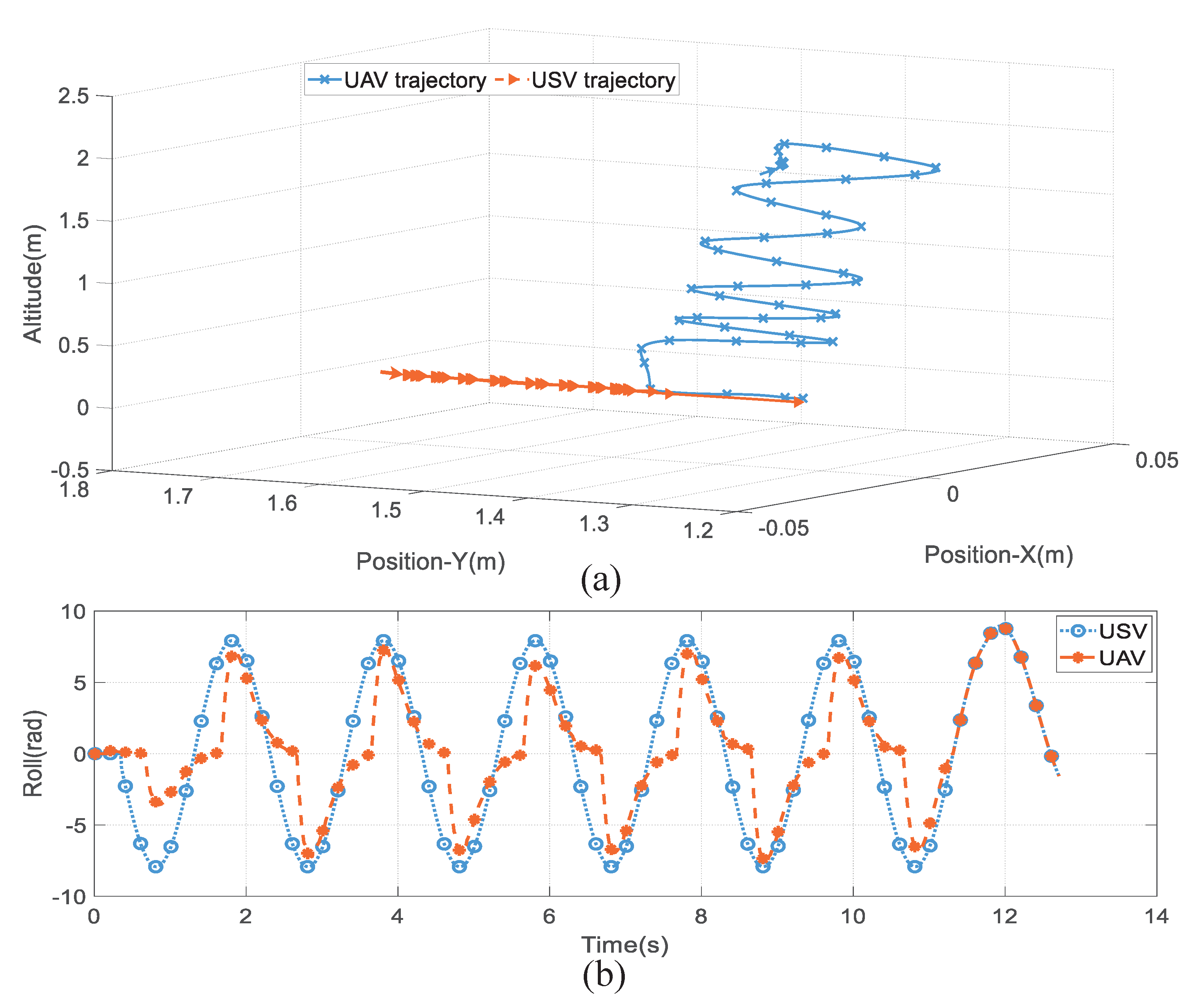
Figure 8.
(a) USV pitching motion−UAV–USV three−dimensional trajectories; (b) the variation of UAV–USV pitch angle.
Figure 8.
(a) USV pitching motion−UAV–USV three−dimensional trajectories; (b) the variation of UAV–USV pitch angle.

Figure 9.
The position change of UAV during landing under USV pitching motion. The UAV can land in pitch motion within 14 s. The landing errors of the UAV final landing point and USV deck center in the direction are m and m, respectively. The two−dimensional Euclidean distance between the UAV’s final landing point and the USV deck center is m.

Figure 10.
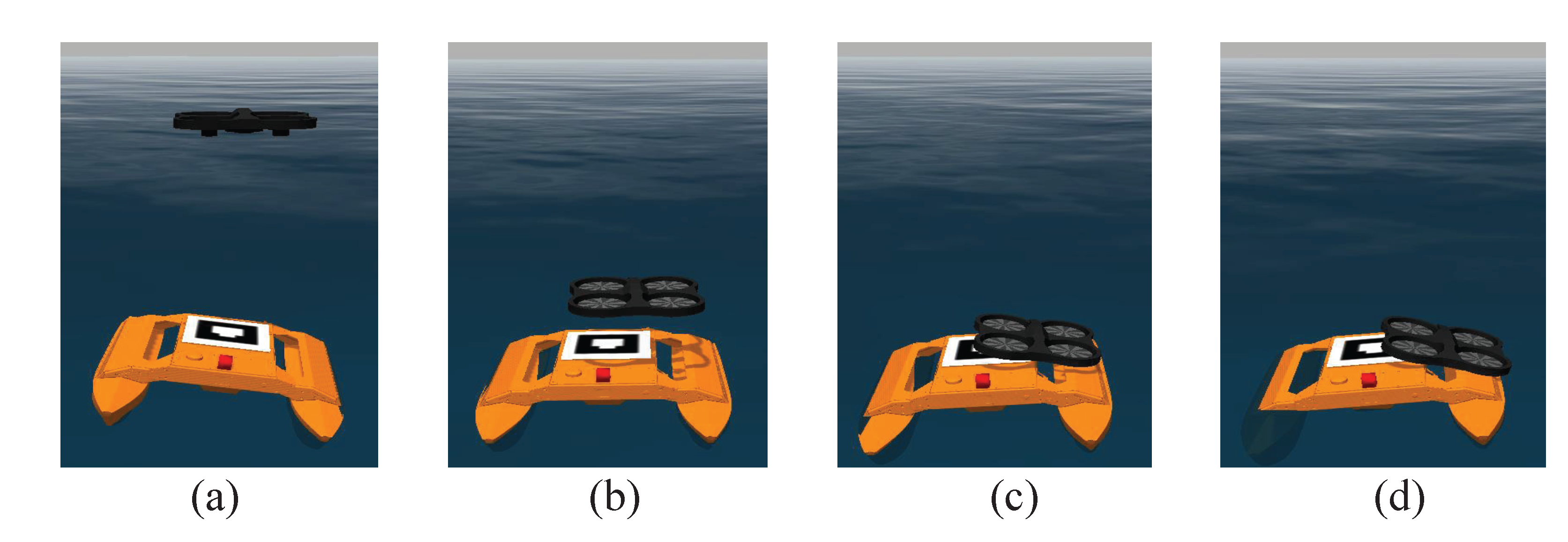
UAV landing autonomously on USV, affected only by USV pitching motion. The UAV altitude does not reach the altitude threshold (set to 2 m), the UAV continues to descend in altitude (a,b); the UAV altitude is less than the altitude threshold , the UAV and the USV attitude remain synchronized (c,d); the UAV altitude is less than the altitude threshold (set to 0.2 m), the UAV accelerates to land on the USV (e); the UAV completes landing on the USV operation (f).
Figure 10.
UAV landing autonomously on USV, affected only by USV pitching motion. The UAV altitude does not reach the altitude threshold (set to 2 m), the UAV continues to descend in altitude (a,b); the UAV altitude is less than the altitude threshold , the UAV and the USV attitude remain synchronized (c,d); the UAV altitude is less than the altitude threshold (set to 0.2 m), the UAV accelerates to land on the USV (e); the UAV completes landing on the USV operation (f).

Figure 11.
Landing accuracy of UAV–USV synchronous movement and conventional movement under the condition of USV pitching motion.
Figure 11.
Landing accuracy of UAV–USV synchronous movement and conventional movement under the condition of USV pitching motion.

Figure 12.
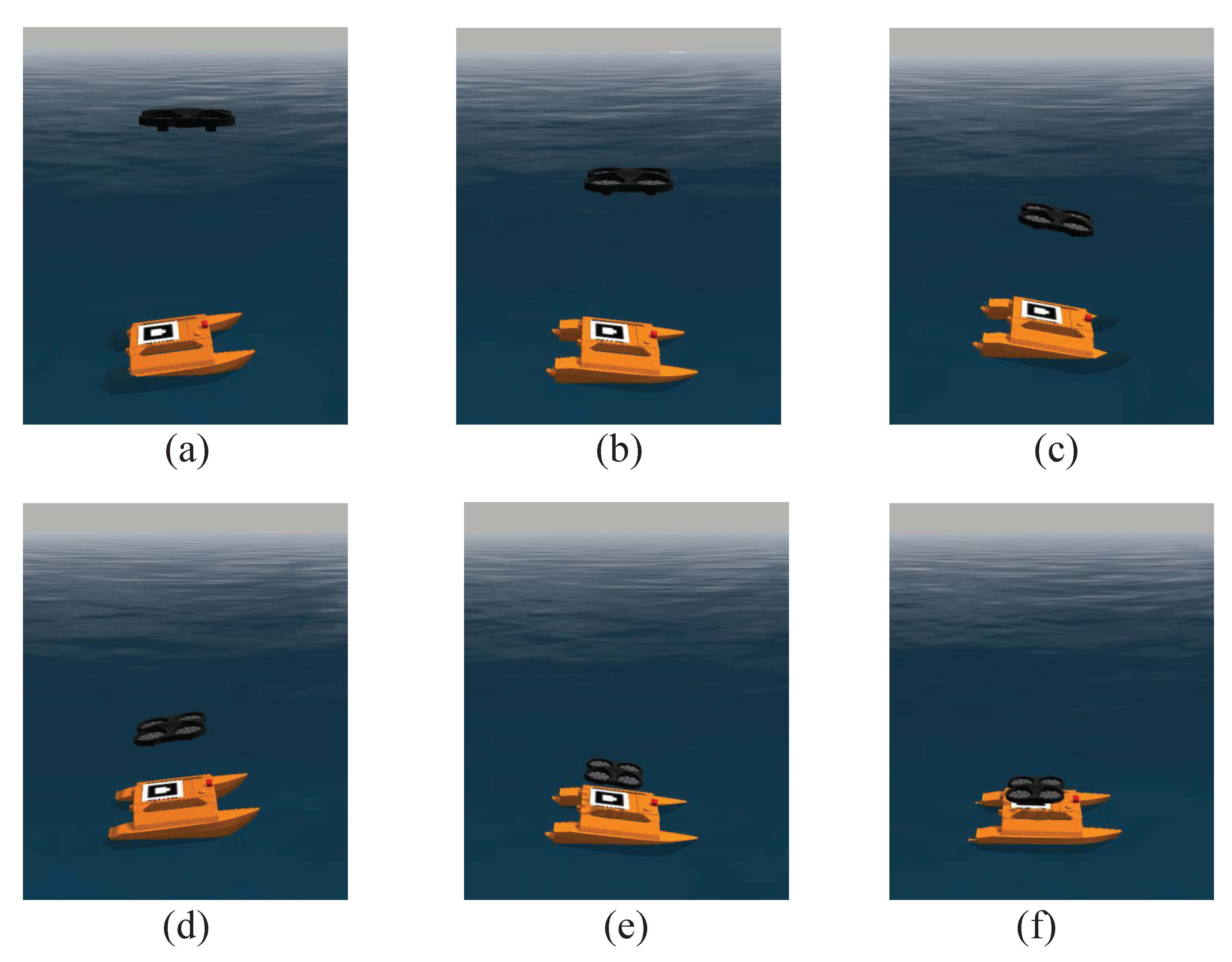
USV roll motion−failure situation of UAV landing.The UAV did not respond to the attitude change of the USV, and the landing process was a vertical landing (a–c). When the USV roll angle changed greatly, the UAV collided with the side of the USV, resulting in the failure of the UAV landing (c,d).
Figure 12.
USV roll motion−failure situation of UAV landing.The UAV did not respond to the attitude change of the USV, and the landing process was a vertical landing (a–c). When the USV roll angle changed greatly, the UAV collided with the side of the USV, resulting in the failure of the UAV landing (c,d).

Figure 13.
(a) USV roll motion−UAV–USV 3D trajectories; (b) the variation of UAV–USV roll angle.

Figure 14.
The position change of UAV during landing under USV roll motion. The landing errors of the UAV final landing point and USV deck center in the direction are m and m, respectively. The two−dimensional Euclidean distance between the UAV’s final landing point and the USV deck center is m.
Figure 14.
The position change of UAV during landing under USV roll motion. The landing errors of the UAV final landing point and USV deck center in the direction are m and m, respectively. The two−dimensional Euclidean distance between the UAV’s final landing point and the USV deck center is m.

Figure 15.
UAV landing autonomously on USV, affected by USV roll motion only. The UAV altitude does not reach the altitude threshold (set to 2 m), the UAV continues to descend in altitude (a,b); the UAV altitude is less than the altitude threshold , the UAV and the USV attitude remain synchronized (c,d); the UAV altitude is less than the altitude threshold (set to 0.2 m), the UAV accelerates to land on the USV (e); the UAV completes landing on the USV operation (f).

Figure 16.
Landing accuracy of UAV–USV synchronous movement and conventional movement under the condition of USV roll motion.
Figure 16.
Landing accuracy of UAV–USV synchronous movement and conventional movement under the condition of USV roll motion.


Table 1.
PID parameters of the UAV controller.
| i | |||
|---|---|---|---|
| 0.4 | 0.01 | 0.3 | |
| 0.4 | 0.01 | 0.28 | |
| 0.02 | 0.01 | 0.001 | |
| Z | 0.5 | 0.05 | 0.2 |
| 0.4 | 0.01 | 0.3 | |
| 0.4 | 0.01 | 0.28 |
Table 2.
Error comparison of USV attitude angle prediction.
| Dataset | Model | RMSE (°) | MAE (°) | MAPE (%) |
|---|---|---|---|---|
| Pitch | LSTM | 0.0050 | 0.0038 | 0.1274 |
| Bi-LSTM | 0.0024 | 0.0020 | 0.1269 | |
| Roll | LSTM | 0.0086 | 0.0067 | 0.6422 |
| Bi-LSTM | 0.0018 | 0.0013 | 0.1054 |
Publisher’s Note: MDPI stays neutral with regard to jurisdictional claims in published maps and institutional affiliations. |
© 2022 by the authors. Licensee MDPI, Basel, Switzerland. This article is an open access article distributed under the terms and conditions of the Creative Commons Attribution (CC BY) license (https://creativecommons.org/licenses/by/4.0/).
Share and Cite
MDPI and ACS Style
Li, W.; Ge, Y.; Guan, Z.; Ye, G. Synchronized Motion-Based UAV–USV Cooperative Autonomous Landing. J. Mar. Sci. Eng. 2022, 10, 1214. https://doi.org/10.3390/jmse10091214
AMA Style
Li W, Ge Y, Guan Z, Ye G. Synchronized Motion-Based UAV–USV Cooperative Autonomous Landing. Journal of Marine Science and Engineering. 2022; 10(9):1214. https://doi.org/10.3390/jmse10091214
Chicago/Turabian StyleLi, Wenzhan, Yuan Ge, Zhihong Guan, and Gang Ye. 2022. "Synchronized Motion-Based UAV–USV Cooperative Autonomous Landing" Journal of Marine Science and Engineering 10, no. 9: 1214. https://doi.org/10.3390/jmse10091214
Note that from the first issue of 2016, this journal uses article numbers instead of page numbers. See further details here.