
YOLO-Submarine Cable: An Improved YOLO-V3 Network for Object Detection on Submarine Cable Images

1
School of Mechanical Engineering, Hangzhou Dianzi University, Hangzhou 310018, China
2
Ocean Technology and Equipment Research Center, Hangzhou Dianzi University, Hangzhou 310018, China
3
School of Cyberspace, Hangzhou Dianzi University, Hangzhou 310018, China
*
Author to whom correspondence should be addressed.
J. Mar. Sci. Eng. 2022, 10(8), 1143; https://doi.org/10.3390/jmse10081143
Submission received: 15 July 2022
/
Revised: 14 August 2022
/
Accepted: 16 August 2022
/
Published: 18 August 2022
(This article belongs to the Special Issue Advances in Autonomous Underwater Robotics Based on Machine Learning)
Abstract
:Due to the strain on land resources, marine energy development is expanding, in which the submarine cable occupies an important position. Therefore, periodic inspections of submarine cables are required. Submarine cable inspection is typically performed using underwater vehicles equipped with cameras. However, the motion of the underwater vehicle body, the dim light underwater, and the property of light propagation in water lead to problems such as the blurring of submarine cable images, the lack of information on the position and characteristics of the submarine cable, and the blue–green color of the images. Furthermore, the submarine cable occupies a significant portion of the image as a linear entity. In this paper, we propose an improved YOLO-SC (YOLO-Submarine Cable) detection method based on the YOLO-V3 algorithm, build a testing environment for submarine cables, and create a submarine cable image dataset. The YOLO-SC network adds skip connections to feature extraction to make the position information of submarine cables more accurate, a top-down downsampling structure in multi-scale special fusion to reduce the network computation and broaden the network perceptual field, and lightweight processing in the prediction network to accelerate the network detection. Under laboratory conditions, we illustrate the effectiveness of these modifications through ablation studies. Compared to other algorithms, the average detection accuracy of the YOLO-SC model is increased by up to 4.2%, and the average detection speed is decreased by up to 1.616 s. The experiments demonstrate that the YOLO-SC model proposed in this paper has a positive impact on the detection of submarine cables.
1. Introduction
Submarine cables, including electric cables, fiber optic cables, and photoelectric composite cables, are laid on the seabed and protected by a reinforced sheath. They have advantages that cannot be obtained by other means in the domains of electrical energy transmission, transoceanic communication, marine engineering, and the development of new energy [1]. With the increasing demand for marine resources in countries around the world, the construction scale of domestic and foreign submarine cables has been expanding [2]. According to research on the submarine cable market, with the construction of 25 additional submarine cables worldwide between 2018 and 2020, they reached a total length of more than 250,000 km. The global submarine cable market had reached 5.14 billion dollars by 2021. Around the year 2000, the first expansion in submarine cable construction began. Typically, submarine cables must be replaced every 20 years. Therefore, the global submarine cable market will enter a new construction period in the next few years, while submarine cable testing will also enter a new phase.
The working environment of the submarine cable is extremely harsh. Natural damage includes long-term erosion by seawater, the impact of ocean currents, fish bites, etc., and human-derived external forces include ship anchorage and fishing. These can result in the damage or even the breakage of the outer protective sheath of the submarine cable, as well as the displacement of the submarine cable position, disrupting the regular operation of the submarine transmission and communication network [3]. In order to ensure that the submarine cable can work properly, regular inspection of the cable condition is essential. Traditional diving detection techniques not only restrict the duration, range, and depth of sea cable detection, but also threaten the diver’s life. Therefore, unmanned and intelligent inspection methods for submarine cables are particularly crucial [4,5,6], among which deep learning-based machine vision detection methods draw the most attention in producing new applications [7,8].
With the development of machine vision, many image-related problems have been solved [9]. In recent years, deep learning [10,11] techniques have increasingly been applied to underwater target detection [12,13], in which convolutional neural networks achieve high accuracy in image classification. Han et al. [14] used deep convolutional neural networks for underwater image processing and target detection with an accuracy of 90%, and the proposed method was applied in underwater vehicles. Li et al. [15] used Faster-RCNN [16] for fish detection and identification. They modified AlexNet [17], making the detection accuracy 9.4% higher than that of the deformable parts model (DPM). Jalal et al. [18] used a combination of a Gaussian mixture model and the YOLO-V1 [19] deep neural network for the detection and classification of underwater species, and their detection F1 score and classification accuracy reached 95.47% and 91.64%. Hu et al. [20] used YOLO-V4 [21] to achieve high detection accuracy for low-quality underwater images and very small targets. They modified the feature pyramid network (FPN) [22] and path aggregation network (PANet) [23] to perform a de-redundancy operation, which increased the average accuracy of the prototype network to 92.61%.
Machine vision inspection is insensitive to underwater noise data, allowing for good environmental information and the ability to identify submarine cables from high-definition, blurred images. Fatan et al. [24] used multi-layer perceptron (MLP) [25] and support vector machine (SVM) [26] to classify the edges of submarine cables. They used morphological filtering and the Hough transform for edge repair and detection, with 95.95% detection accuracy. However, they only used this method to detect the straight line of the cable, and it does not have a good detection effect on blurred cable pictures. Stamoulakatos et al. [27] used a deep convolutional neural network (ResNet-50) to detect submarine pipelines under low light, with accuracy of 95% to 99.7%. However, they use a two-stage detection network, which has a long average detection time and fails to meet the requirements when performing real-time detection. Balasuriya et al. [28] used visual detection to solve the problem of the partial absence of submarine cables and selection when multiple submarine cables are present at the same time. Finally, the position of the submarine cable was inferred by combining the position information of an autonomous underwater vehicle (AUV). Chen et al. [29] considered the poor quality of underwater images due to underwater scattering and absorption characteristics. They preprocessed the images by enhancing the original contrast memory grayscale and finally extracted the edge of the sea cable by mathematical morphological processing and edge detection. However, their method is not applicable to the case of complex backgrounds and will lead to the difficulty of submarine cable edge extraction and low recognition accuracy.
The underwater images [30,31] of the submarine cables are always blurred and blue–green [32,33], which makes the position and feature information difficult to extract. In this paper, the YOLO-SC network based on the improved YOLO-V3 [34] network is proposed. The detection model improves the detection accuracy while simplifying the prediction network structure and shortening the average time of detection. The main contributions of this article are listed as follows:
(1) A target detection model is proposed for submarine cables to fill the gaps in the current research domain for submarine cable detection. The proposed YOLO-SC model outperforms other network models that have been applied to underwater target detection.
(2) An image preprocessing method is added in front of the feature extraction module to enhance the performance of detection. The method can effectively solve the problem of difficult feature extraction due to the blue–green color of underwater images of submarine cables.
(3) Skip connection [35] and multi-structured multi-size feature fusion are added in feature extraction and feature fusion, respectively, to solve the problem of insufficient position information and feature information of submarine cable targets due to blurred images.
(4) A lightweight prediction network is proposed based on the slightly larger proportion of submarine cables in the image, which shortens the detection time of the model and can meet the standard of real-time detection underwater.
(5) A diversity submarine cable dataset was created to supply the data for the study of submarine cable object recognition. Our image dataset contains 3104 images with different disturbances, such as motion blur, partial absence, occlusion, absorption, and scattering effects of water on light.
The rest of this paper is organized as follows: Section 2 describes submarine cable image preprocessing, including several algorithms for image data enhancement. In Section 3, the YOLO-V3 network and the proposed YOLO-SC network, which is based on an improved YOLO-V3 prototype network, are described. The model’s assessment via experiments is discussed in Section 4. Section 5 presents the conclusions and future work.
2. Image Dataset Production
Due to the complexity of the subsea working environment of the submarine cable, the low integrity of the dataset has negative effects for the neural network detection results. In order to improve the richness of the experimental dataset, the images of the dataset are preprocessed [36] with image brightness, color, and rotation, and the data of the submarine cable images are expanded to 4798 images in this paper. The specific data are shown in Table 1.
2.1. Image Brightness
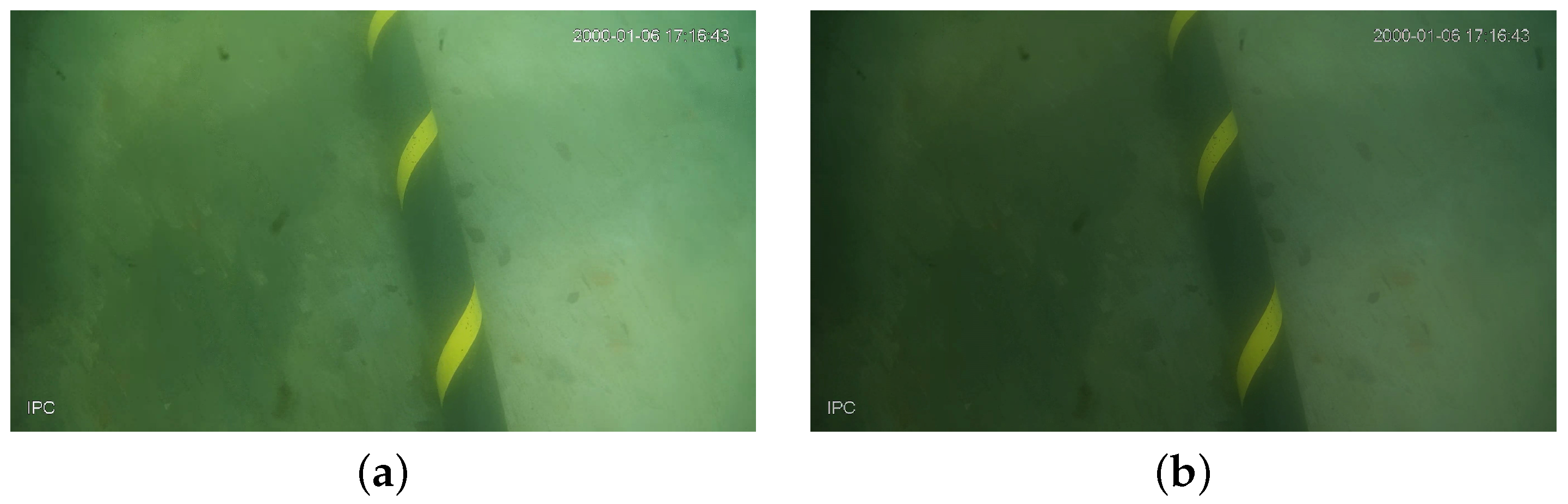
The illumination conditions of the seafloor are constantly changing with the distance from the sea level, and the illumination conditions of the submarine cable images are also constantly changing. In order to more accurately simulate the situation of the submarine cable, the brightness of the images in the training set will be processed as follows. We choose a random value from the lowest () to the highest () value of the brightness of each image, and this value will replace the original brightness of the image. However, this may cause the images to be too dark or too bright, which in turn may cause the neural network to generate error messages when training these images. In this paper, it is set to 1.2 times the lowest value of the original brightness and is set to 0.8 times the highest value of the brightness, which can simulate the situation of the submarine cable under different levels of illumination and compensate for the incompleteness of the experiment [37]. Some of the sample brightness transformations are shown in Figure 1.
2.2. Image Color
Light striking an object is reflected and reaches the human eye to appear as the object itself. When we see objects on land, the medium through which the light passes is air. When taking photos underwater, water acts as the medium for light transmission, and water has an absorption and scattering effect on light. When an object passes through the medium of water and reaches the human eye or an optical sensor, the object loses its color and mostly appears blue–green. Automatic White Balance (AWB) is a very important concept in the field of imaging. The algorithm can solve the image color reproduction problem and tone balance problem to some extent. It can correct or eliminate the underwater environment due to external natural light, water absorption of light or the camera system comes with lighting equipment and color bias, in order to keep the image color constant. Nowadays, the main automatic white balance algorithms are the Gray World Method [38], Perfect Reflector Method, etc. Therefore, in this paper, the Gray World Method algorithm was used to color balance the images in the training set. The steps of the algorithm are as follows:
(1) The mean values of the three channels R, G and B are found. The formula is as follows:
(2) The obtained R, G and B channel means are summed and divided by the number of channels. In this way, the grayscale mean value of the image is obtained. The equation is as follows:
(3) The image grayscale values are divided by R, G, B three channel average value, and then obtain the R, G, B three channel gain coefficient. The formula is as follows:
(4) The gain coefficients of the R, G and B channels are multiplied with the gray values of the corresponding pixels of the R, G and B channels of the input images, respectively. Finally, the automatic white balance result is obtained. The formula is as follows:
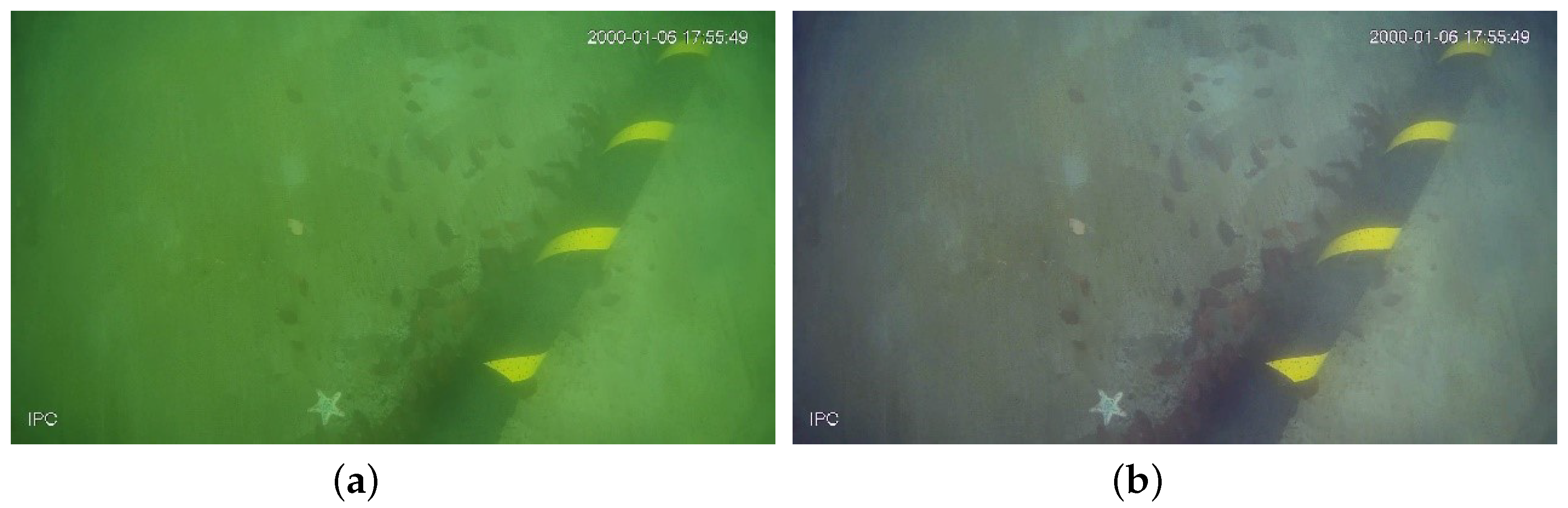
Some of the sample color balance treatments are shown in Figure 2.
2.3. Image Rotation
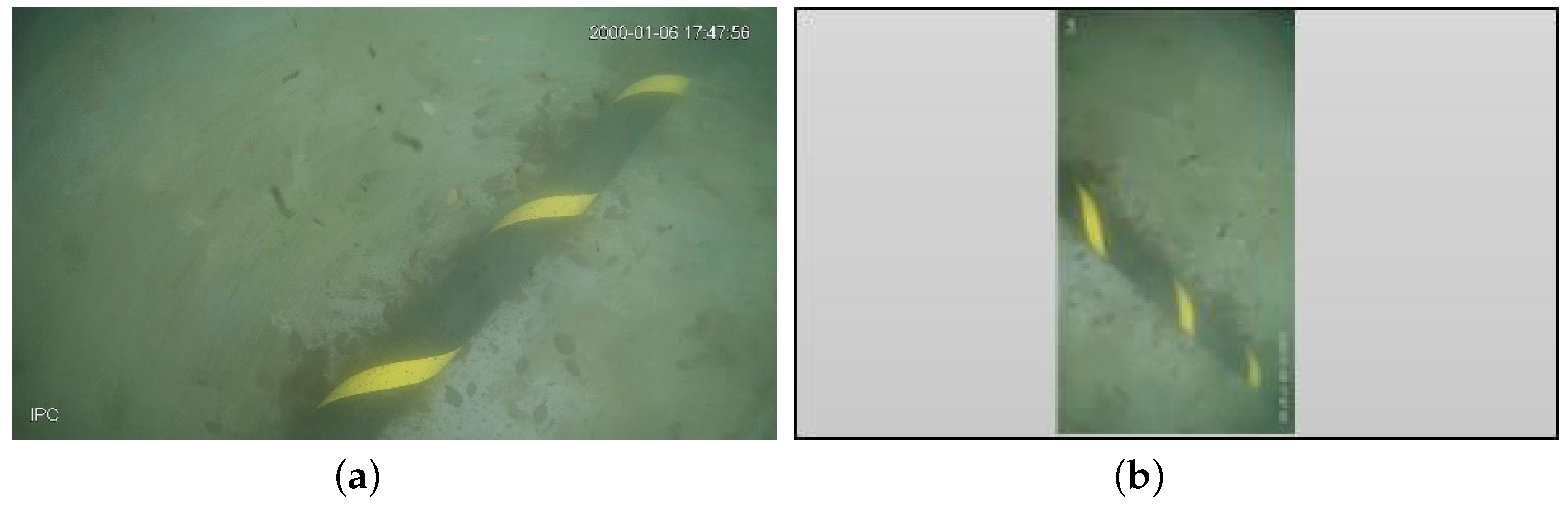
Image rotation can further expand the submarine cable image dataset, and the rotated images can also improve the detection performance of the neural network. In this paper, the image dataset of the submarine cable is acquired, and all rotation angles of the cable are presented. We only need to rotate the original image clockwise . Since the length and width of the image are swapped after rotation, this paper will change the image size to a fixed size () before the image is input to the neural network. A grayscale bar is added around the image, which can ensure that the image is not distorted. Some of the samples were rotated clockwise for processing, as shown in Figure 3.
3. Proposed Submarine Cable Target Detection Method
3.1. YOLO-V3
YOLO is short for “You Only Look Once”. The YOLO-V3 network is adapted from the YOLO-V1 and YOLO-V2 [39] networks. In order to solve the problem of the low detection rate of small target detection in the YOLO-V1 and YOLO-V2 networks, the YOLO-V3 network sacrifices some running time. The accuracy rate of detection has been improved significantly. YOLO-V3 belongs to the family of one-stage detection algorithms, which directly transform the detection problem into a regression problem. It has a faster detection speed. However, compared with the two-stage detection algorithm Faster-RCNN, the recognition accuracy and precision are generally slightly worse.
The network structure of YOLO-V3 is shown in Figure 4. It is composed of four modules, namely, the input module, feature extraction network, cross-scale feature fusion network, and prediction network. Input is a RGB image. In the feature extraction network, the network structure is deepened by using simplified residual blocks instead of the original and blocks, turning the original Darknet-19 into Darknet-53. In the prediction network, multi-level prediction is used to solve the problem of coarse granularity. Regarding the detection of small targets, it will output three scales of output. These three scales correspond to the detection of small, medium, and large targets, and it finally outputs the class and border of each target object. YOLO-V3 uses the logistic loss function as a new loss function compared to its predecessor, allowing YOLO-V3 to classify and frame overlapping regions.
3.2. Proposed YOLO-SC Model
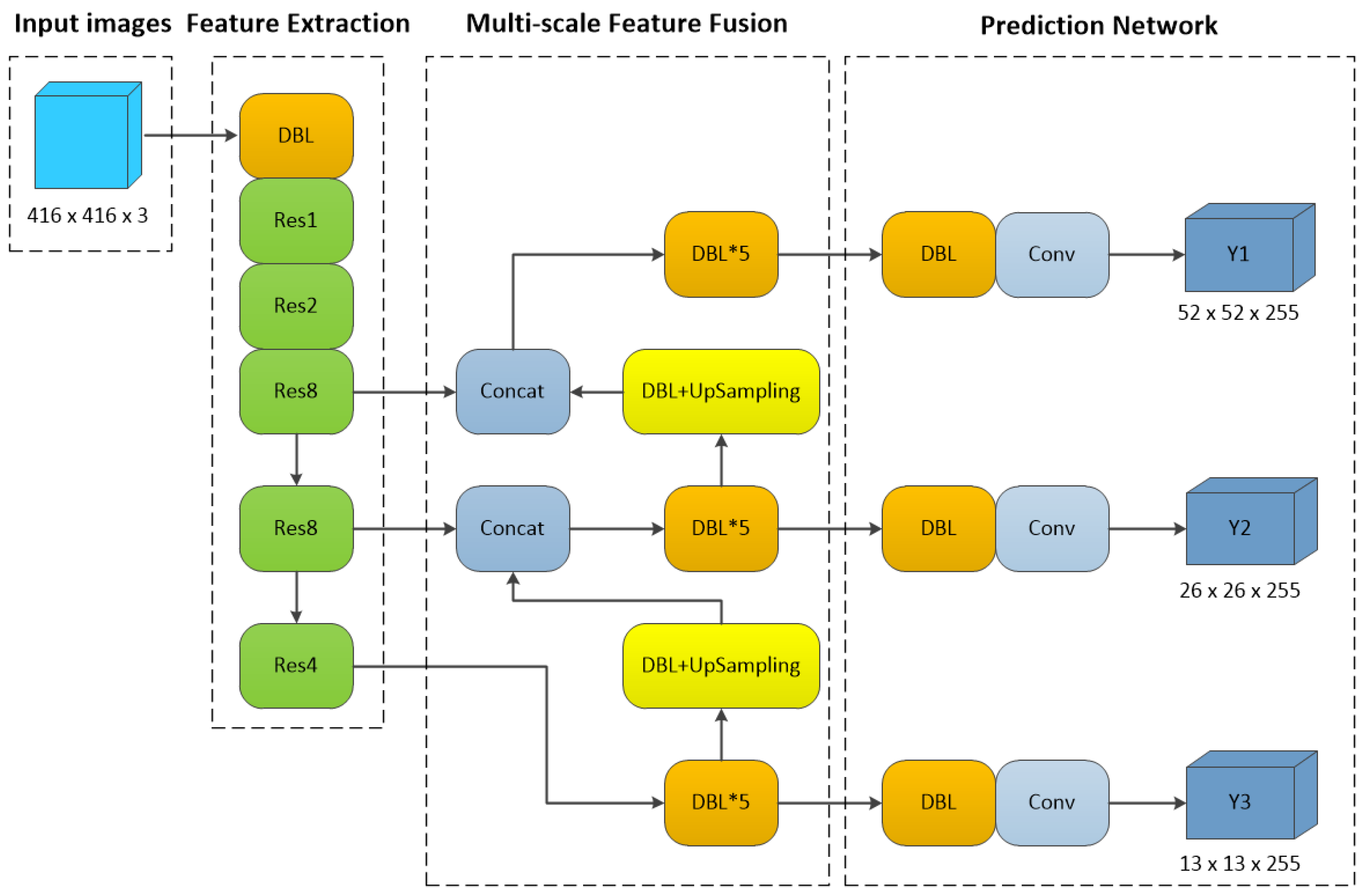
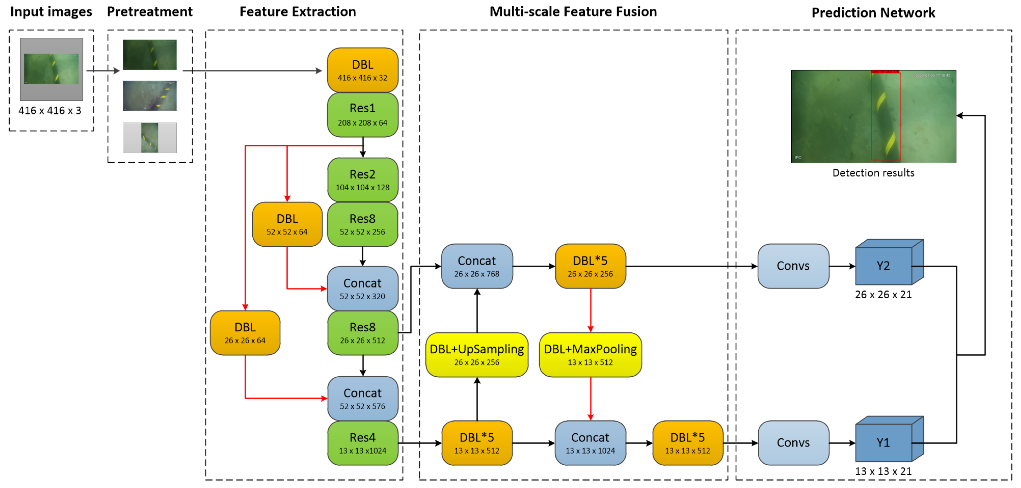
An overview of the proposed YOLO-SC network structure is shown in Figure 5. With deeper convolution, the higher-level feature semantic information is richer in the YOLO-V3 network, but the position information of the target is missing [40]. In the feature extraction network, skip connections are added in this paper to enhance the target position information at higher levels. In this paper, considering the complexity of underwater pictures, both feature information and position information of the target are very important. Therefore, in the multi-scale feature fusion network, this paper borrows from [41] and uses top-down upsampling and bottom-up downsampling (maximum pooling) combined.
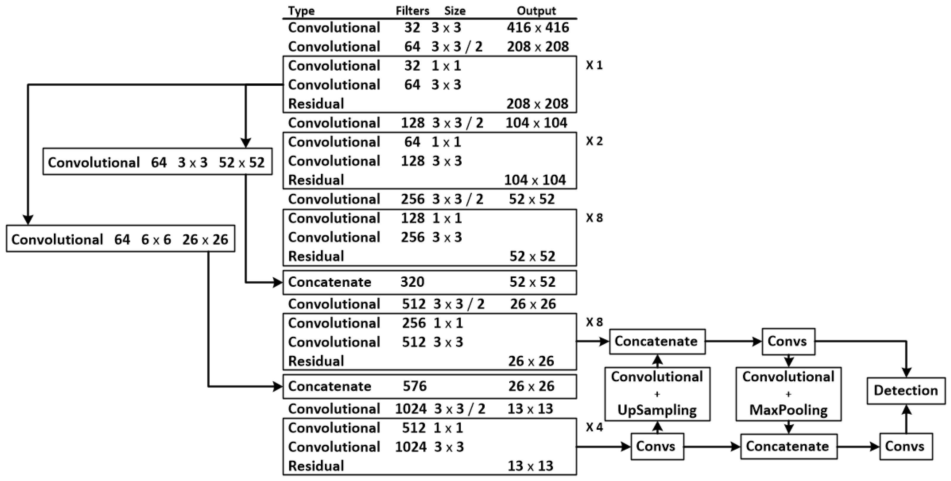
This structure transmits the high-level semantic information to the bottom output network with insufficient feature information by upsampling, and the bottom position information to the top output network with insufficient position information by downsampling. In the prediction network, this paper takes into account that the submarine cable is in the shape of a line, which takes up a slightly larger proportion of the whole image. Therefore, in order to speed up the network detection, the branches used to detect small targets in the prediction network are removed in the proposed network architecture. This will make the network lightweight. The YOLO-SC network parameters are shown in Figure 6.
3.3. Skip Connection to Enhance Position Information
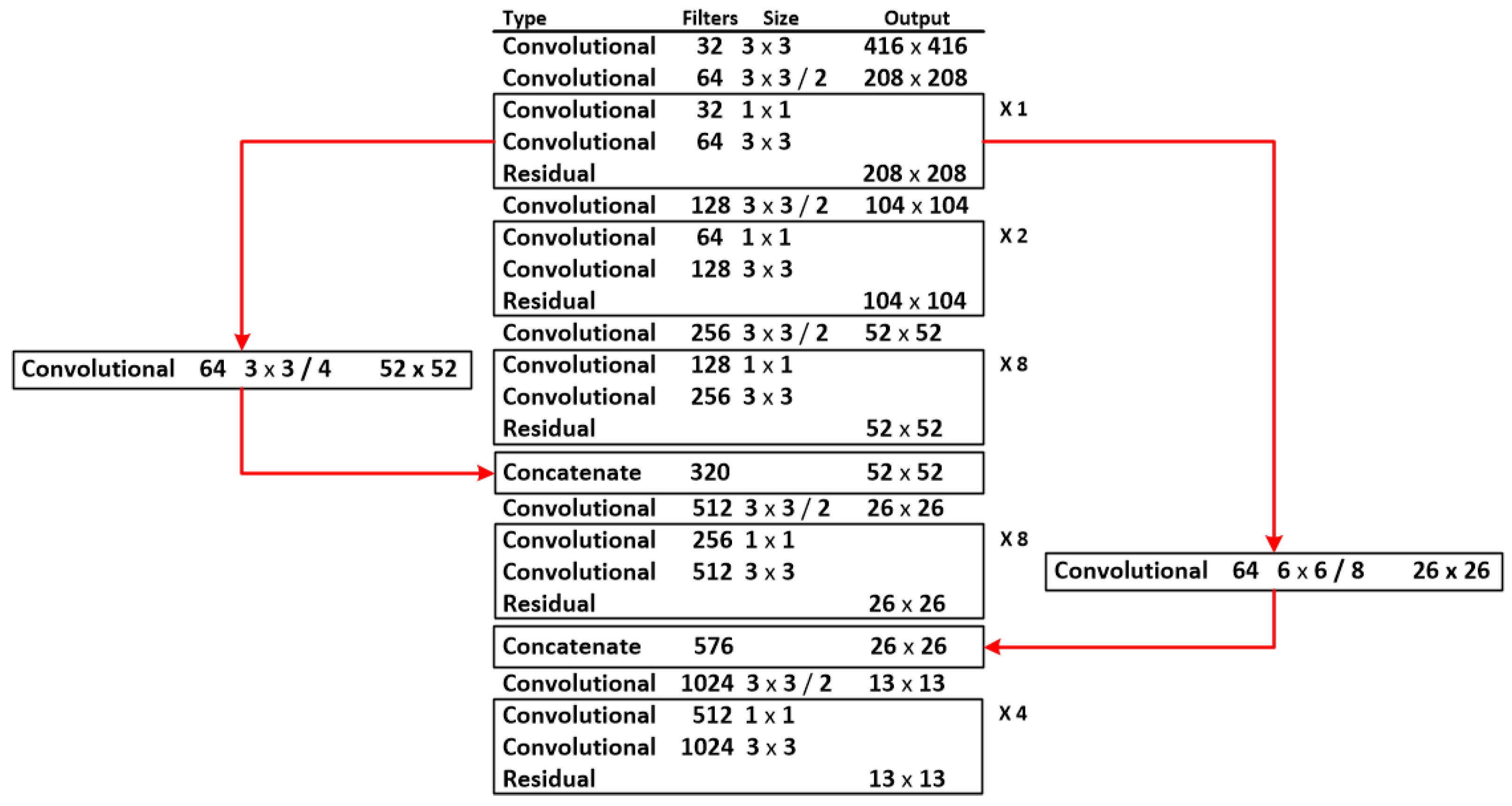
With the deepening of the convolution degree, the semantic information of the high-level features is richer, but the position information of the target is missing [40]. In this paper, the following improvements have been made to solve this problem. In the feature extraction module, the residual blocks in the first layer belong to the underlying feature layer, which has good information about the target position. The fourth and fifth layers belong to the higher-level feature layers, which have good feature semantic information. In this paper, the first layer of residual blocks is convolved once with a kernel size of and a step size of 4, and once with a kernel size of and a step size of 8, respectively. This will result in two feature layers, one with a size of and a number of channels of 64, and the other with a size of 26 × 26 and a number of channels of 64. These two feature layers are rich in target position information. The feature layer of size is connected to the output of the residual block of the third layer, and the new feature layer formed is used as the input of the fourth layer.
The feature layer of size is connected to the output of the residual block of the fourth layer, and the new feature layer formed is used as the input of the fifth layer.
Thus, the feature layers output by the residual blocks in the fourth and fifth layers are not only rich in feature semantic information, but also contain good target position information. The specific network parameters of the skip connection are shown in Figure 7.
3.4. Lightweight Predictive Networks
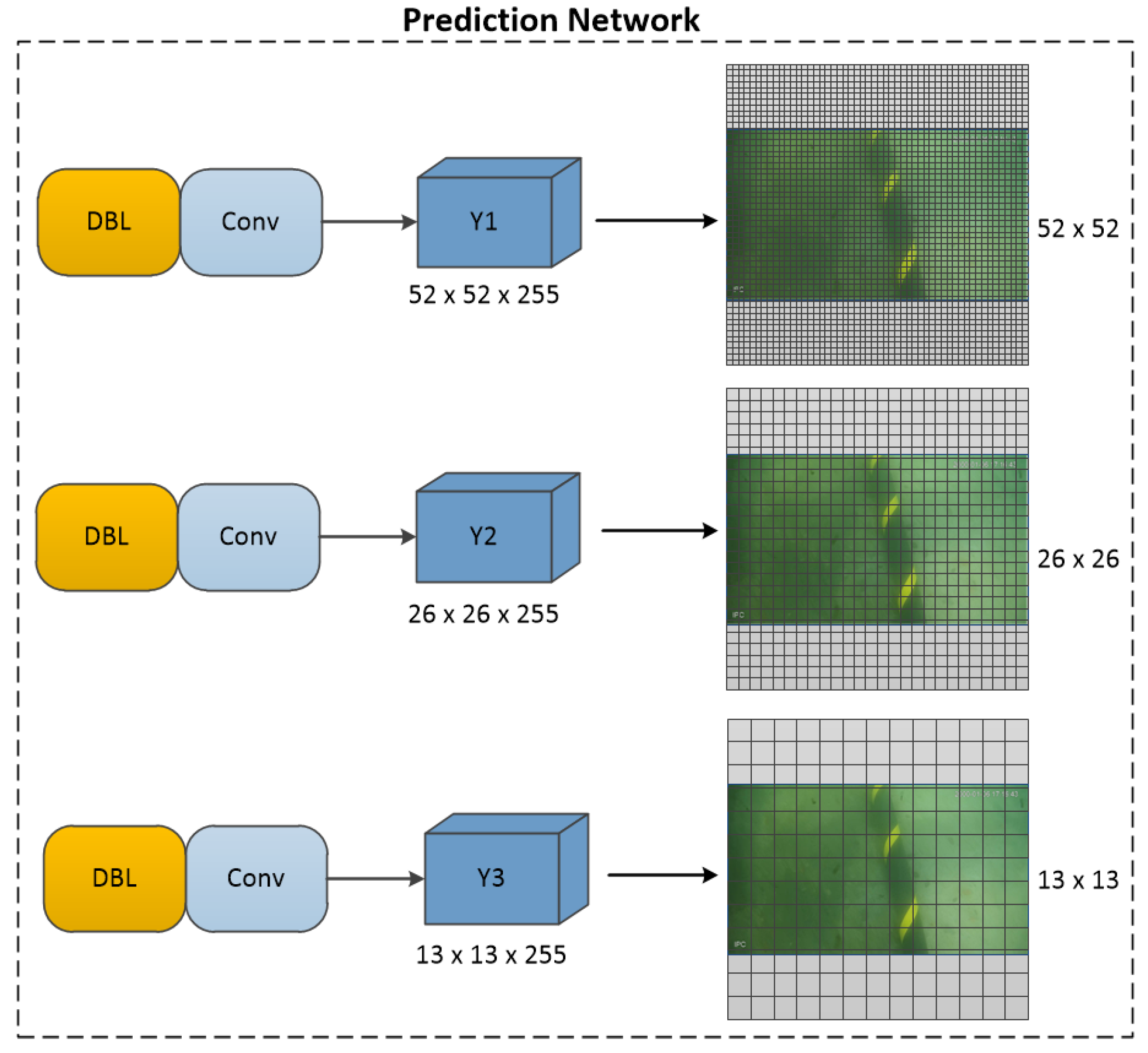
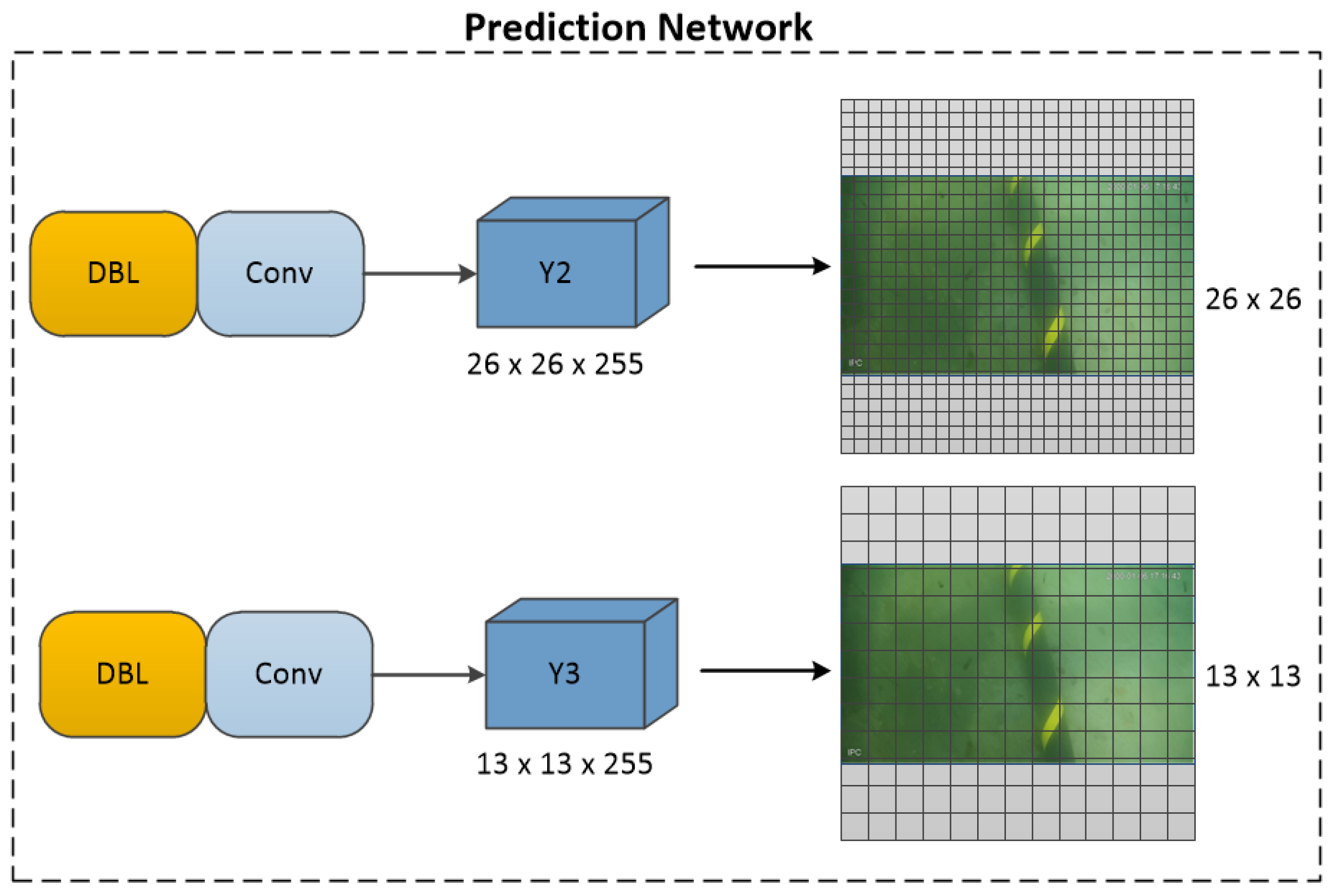
The prediction network of YOLO-V2 is changed from of YOLO-V1 to . The prediction network of YOLO-V3 is an improvement over YOLO-V2. It divides the prediction network into three branches, dividing the images into , , and grids. The three grids are used for the detection of large, medium, and small targets, respectively. The YOLO-V3 prediction network structure is shown in Figure 8. Since the submarine cable is considered to have a line shape and a slightly larger proportion in the image, in this paper, the branches used to detect small targets are removed. The method can reduce unnecessary network computations, reduce the weight of the overall network structure, and speed up network prediction. The YOLO-SC prediction network structure is shown in Figure 9.
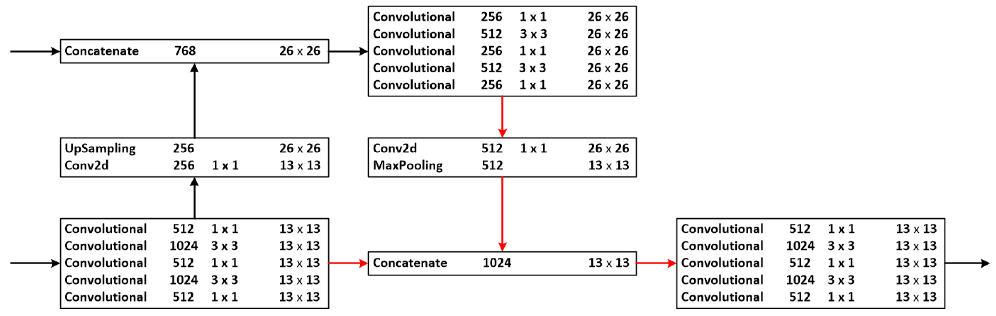
3.5. Multi-Scale Feature Fusion for Multiple Structures
As noted in the previous section, the branch used to detect small targets in the YOLO-V3 prediction network is removed in this paper. This reduces the computation of the network, but may bring about insufficient overall network feature extraction. For this reason, we describe how to solve this problem in this section. A multi-structured multi-scale fusion network is shown in Figure 10. Based on the prototype network of YOLO-V3, the output feature layer of the fifth residual block is convolved five times, and the convolved feature layer is input to two branches, respectively. The first branch is used as an input for multi-scale feature fusion. The second branch first performs a convolution with a kernel size of to reduce the number of channels, and then changes the feature layer size to by an upsampling operation. The new feature layer is then used for multi-scale feature fusion with the output feature layer of the residual block of the fourth layer.
The feature layer of size and channel number 768 is obtained, and this feature layer is convolved five times to obtain a feature layer of size and channel number 2568. Then, a convolution kernel of size is used to boost the number of channels, and the feature layer size is changed to by a maximum pooling operation. Finally, it is fused with the first branch for multi-size features and inputs to the prediction network.
Through a series of operations, this paper combines top-down upsampling and low-up upsampling (maxpooling). First, the maxpooling layer from low to high can reduce dimensionality, remove redundant information, reduce computational effort, and expand the receptive field of the high-level feature layer. Second, the newly added five convolution operations increase the feature semantic information of the prediction network used to detect large targets. Finally, the overall structure compensates for the lack of feature information caused by the removal of small target detection.
3.6. Loss Function of the YOLO-SC Model
The loss function of YOLO-V3 is an improvement on YOLO-V1 and YOLO-V2, which changes the classification prediction to regression prediction. The classification loss function becomes a two-to-cross-entropy loss function. The loss function of the YOLO-SC model proposed in this paper is defined as follows:
Firstly, the images are divided into grids, and M anchor boxes are generated within each grid. Each prior frame will be trained by the model, and finally the corresponding prediction frame is obtained, with the median coordinate loss defined as follows:
where i and j denote the j-th anchor box in the i-th grid, and x and y denote the coordinates of the center point.
The loss of width and height coordinates is defined as follows:
where denotes whether the j-th anchor box in the i-th grid contains the target object. It is set to 1 if it contains the object; otherwise, it is set to 0. w and h denote the width and height of the anchor box.
Confidence loss is defined as follows:
where C denotes the confidence that the object inside the anchor boxes belongs to the target object. denotes whether the j-th anchor box inside the i-th grid does not contain the object. It is set to 1 if it does not contain the object; otherwise, it is set to 0. denotes the weight of the lost part without the object, so that the calculation of the absence of the object can be reduced and the network tends to detect the grid with the object.
Classified loss is defined as follows:
where denotes the category when the j-th anchor box in the i-th grid is responsible for the target object.
In order to verify the effectiveness of the proposed YOLO-SC model for submarine cable detection, a series of evaluations of the model are carried out in this paper. The relevant metrics to evaluate the performance of the neural network model are as follows:
(1) The most relevant metrics to evaluate the trained model are and , as follows:
Among them, the details of (True Positives), (True Negatives), (False Positives), and (False Negatives) are shown in Table 2. Precision indicates the ratio of the number of correctly assigned positive samples to the total number of assigned positive samples. Recall indicates the ratio of the number of correctly assigned positive samples to the total number of samples.
(2) (average precision) is used to measure how well the trained model performs on each class and is defined as follows:
where n denotes the number of detection points and denotes the value of accuracy at a recall of r.
(3) The F1 score is the sum average of precision and recall, and is used to evaluate the overall performance of the model. F1 score is defined as follows:
4. Experiment and Discussion
This section is divided into four parts. The first part introduces the experimental setup; the second part shows the experimental results of the YOLO-SC model on the submarine cable dataset; the third part compares the performance of the proposed YOLO-SC model with other algorithms; and, finally, the YOLO-SC model is studied for ablation.
4.1. Datasets and Experimental Settings
4.1.1. Image Data Acquisition
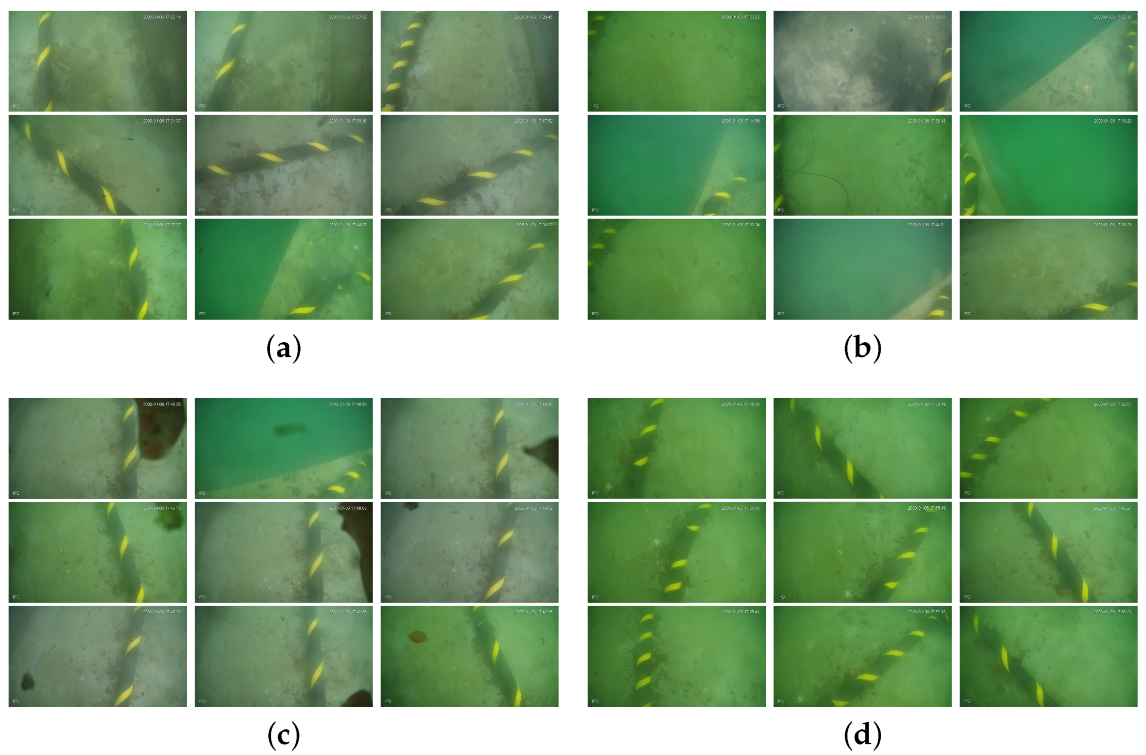
The submarine cable dataset used in this paper was collected at the pool test site of Hangzhou Dianzi University (Dongyue Campus). The submarine cable body was simulated with PVC pipe according to the real submarine cable. Images were taken with a deep-sea high-definition and high-frame-rate network camera jointly developed by Dahua and Hangzhou Dianzi University, with a resolution of 2688 × 1520 pixels. A total of 3104 images were taken, including 2399 images of the target object of the submarine cable. All the images were taken under natural conditions, including some disturbing factors: motion blur, partial absence, occlusion, absorption, and scattering effects of water on light. Some samples of the dataset under different disturbances are shown in Figure 11.
4.1.2. Image Annotation and Dataset Production
In this paper, the acquired image data are firstly filtered to eliminate the images without the target object of the submarine cable. Secondly, the filtered images are subjected to image data enhancement, after which each image is numbered. The numbered images are manually annotated and the submarine cable target object is selected with a horizontal frame. Finally, the annotated images are converted to PASCAL VOC format so that they can be easily compared with the performance of other algorithms. It is randomly divided into a training set, a validation set, and a test set. The training set consists of 3886 images, the validation set consists of 432 images, and the test set consists of 480 images of the original image. The ratios are as follows:
The specific parameters of the , , and are shown in Table 3.
4.1.3. YOLO-SC Model Initialization Parameters
The YOLO-SC model for this experimental study was trained and tested on a desktop computer. The hardware parameters are shown in Table 4. The whole model is built on the pytorch platform. The programming language and software used are Python and pycharm, respectively. The pixel size of the input image of this model is bit . Considering the effect of CPU memory, the batch size is set to 8 in this paper. The model is trained for 100 epochs, and other initialization parameters, such as momentum and initial learning rate, are shown in Table 5.
4.2. Experimental Results of YOLO-SC Model on Submarine Cable Dataset
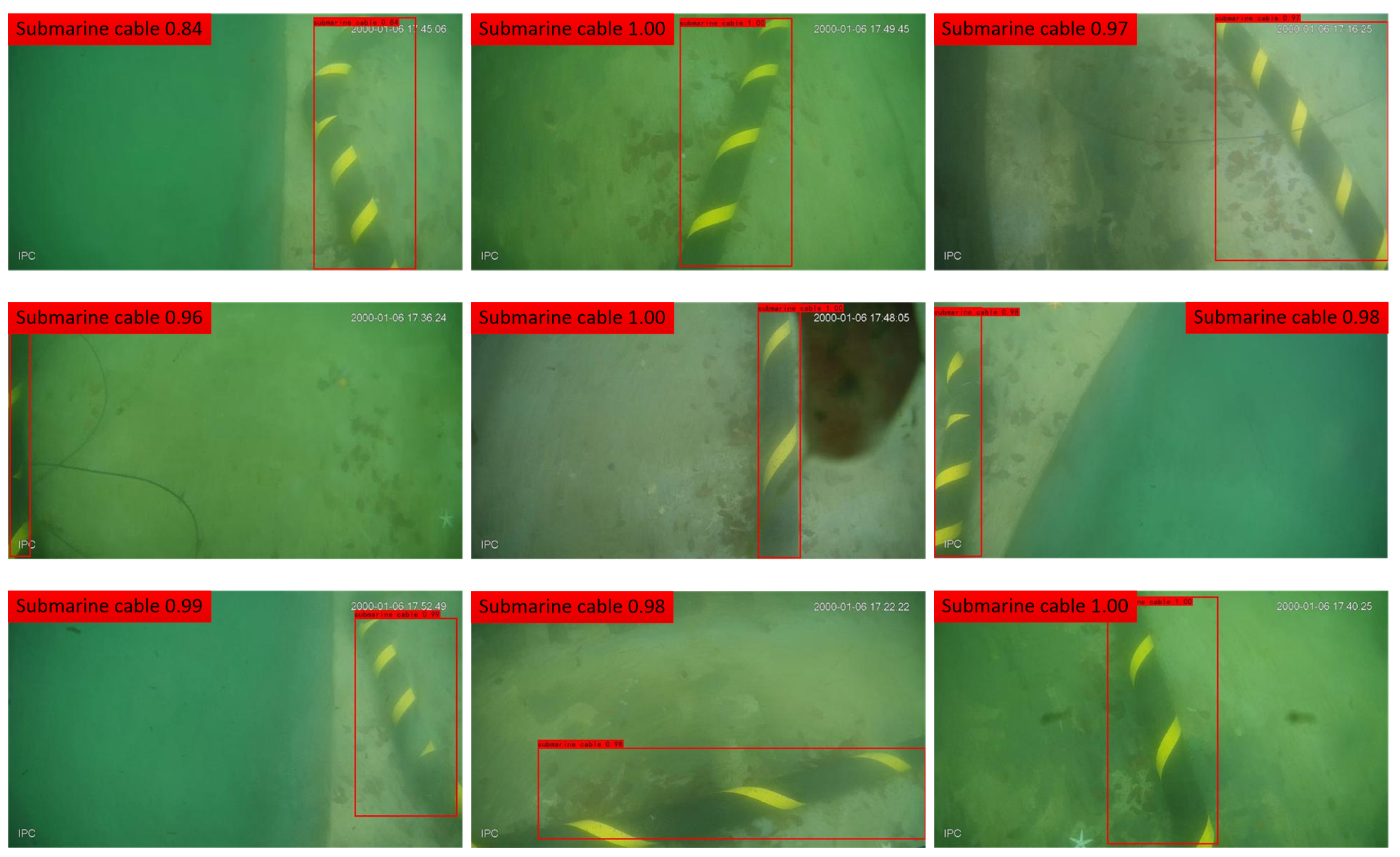
In this paper, the YOLO-SC model is obtained after completing the improvement of the YOLO-V3 model. After training the YOLO-SC model, it is applied to the test set of the submarine cable dataset and measured result of submarine cable detection are obtatined. Some of them are shown in Figure 12. These images have a pixel size of . The red part of the figure shows the confidence of the prediction box, while is enlarged next to it because the font size is too small.
From the measured results, the detection rate of the YOLO-SC model for submarine cables is high. The confidence score of straight submarine cables can ultimately reach above 0.97. The model also has good performance for bent submarine cables and submarine cables with occlusion in the images.
4.3. Comparison of Different Algorithms
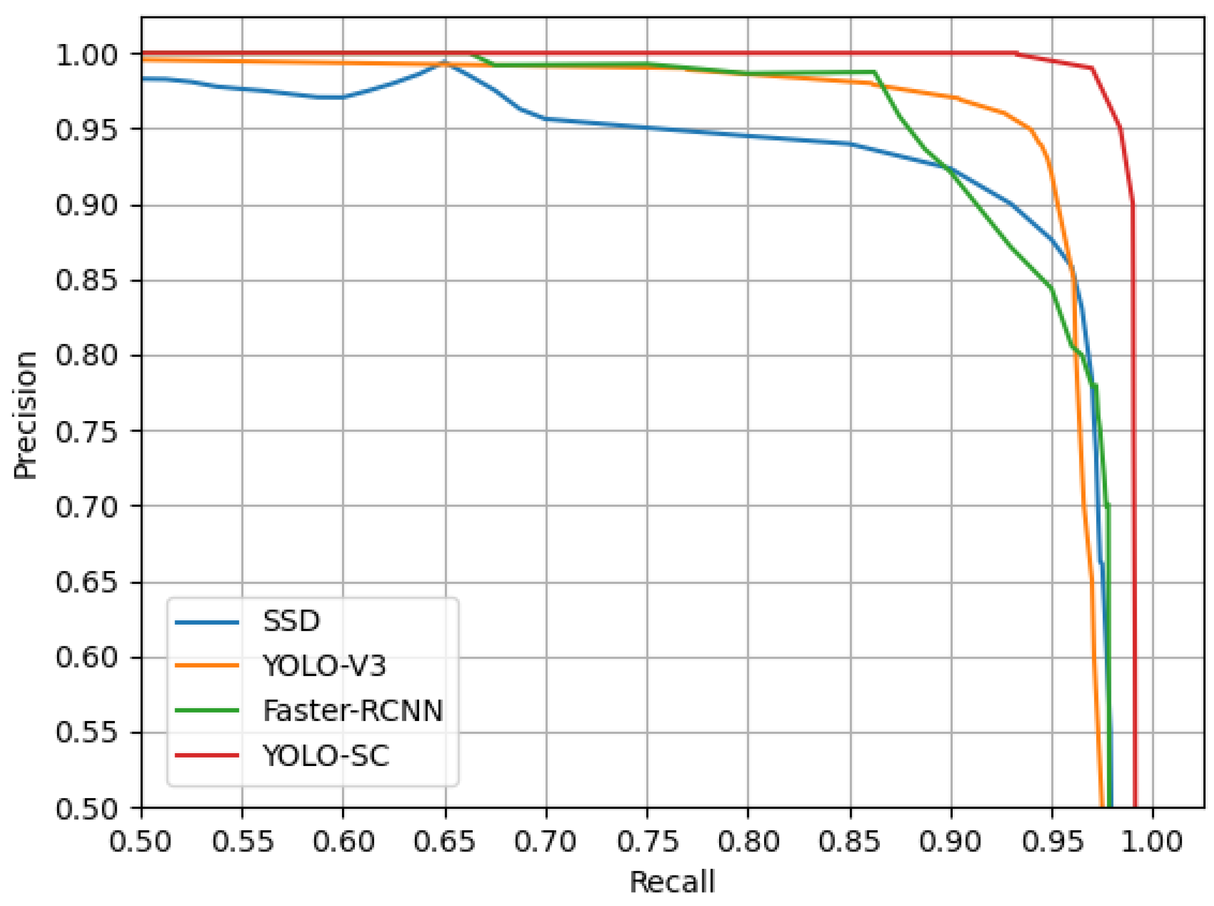
To further validate the effectiveness of the submarine cable detection model proposed in this paper, the proposed YOLO-SC model is compared with models that have been applied in underwater target detection (YOLO-V3, SSD [42], and Faster-RCNN) in terms of average detection accuracy, F1 score, and detection speed, with a consistent dataset and confidence threshold (0.8). The results are shown in Table 6. The precision–recall curves (P-R curves) for the different models are shown in Figure 13.
According to the experimental results, it can be seen that the YOLO-SC model proposed in this paper has the best performance among all the above models. The average time of SSD model detection is the lowest, but its detection accuracy is also the lowest. SSD is a one-stage detection algorithm that localizes and classifies the target only once, so it has a short average detection time. It performs convolution on the feature map to detect the target, not using fully connected layers. Therefore, it loses a great deal of spatial information and has lower average detection accuracy. YOLO-V3 has medium detection accuracy and average time. The detection accuracy of the Faster-RCNN model is higher than that of the YOLO-V3 model, but its average detection time is up to 2.068 s, which does not allow for the real-time detection of underwater targets. Finally, the detection accuracy of the YOLO-SC model proposed in this paper is the highest, with an AP of 99.41% and an average time of 0.452 s, indicating that it can achieve the real-time detection of underwater targets. The effectiveness of the YOLO-SC model proposed in this paper is further verified through the comparison of different algorithms.
4.4. Impact of Data Enhancement Methods on Detection Models
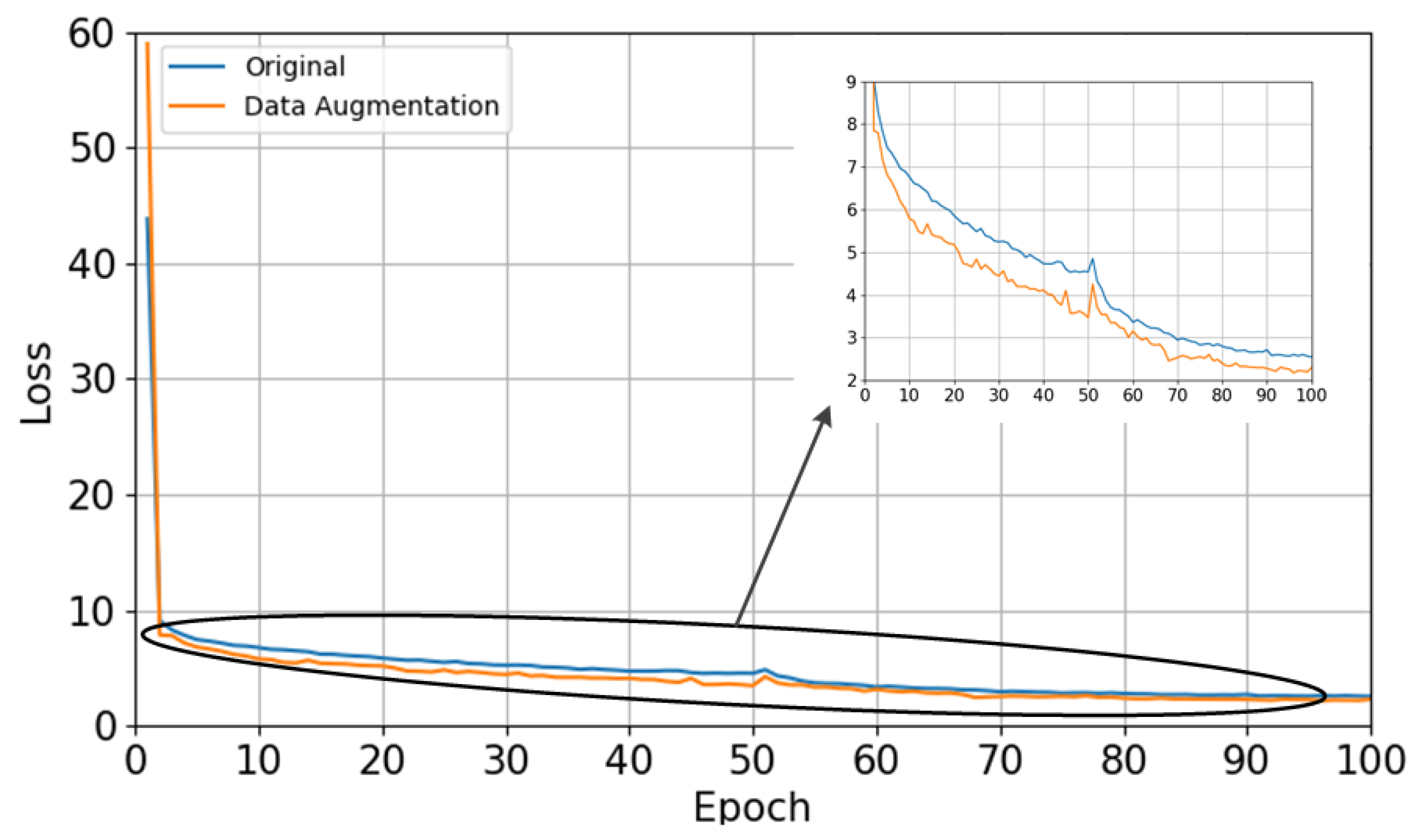
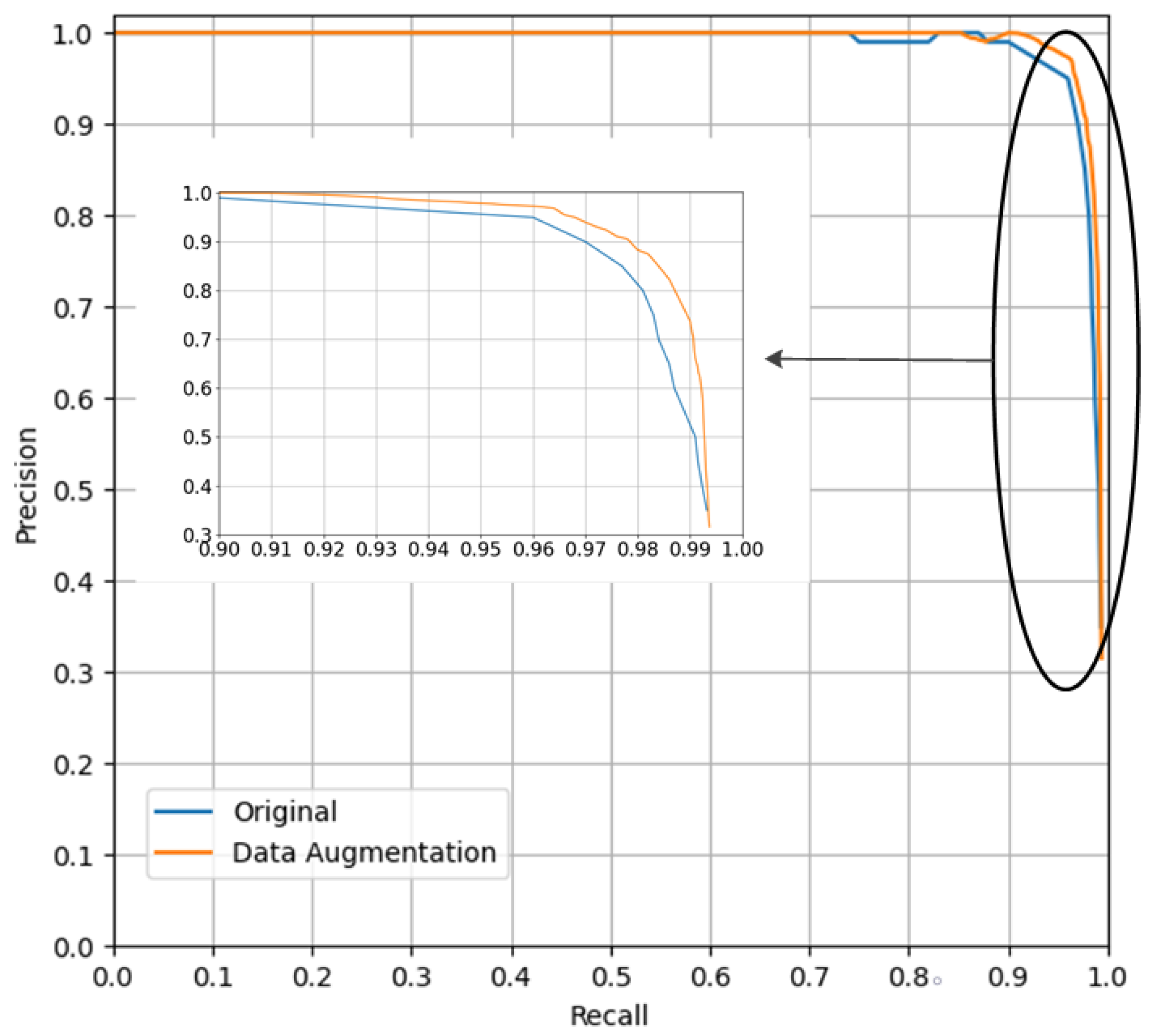
In this paper, the luminance transformation, color balance, and rotation transformation methods of data enhancement are used to enhance the image dataset. Since underwater images are strongly influenced by the absorption and scattering of light by water, this paper analyzes the effect of the data enhancement methods on the inspection model. Firstly, the original submarine cable image is used as the original dataset, The original image data set is randomly divided into three equal parts for brightness transformation, color balance and rotation transformation operations respectively, and the enhanced cable images are used as the enhanced data set after data enhancement. Secondly, the two datasets are input to the YOLO-SC model for training. Finally, the results of the effect of the two datasets on the detection model are obtained. The loss curves and precision–recall curves (P-R curves) of the YOLO-SC model for the two datasets are shown, respectively, in Figure 14 and Figure 15. The average precision (AP) and F1 scores of the YOLO-SC model for the two datasets are shown in Table 7.
As can be seen in Figure 14, the data-enhanced dataset is trained on the YOLO-SC model and the model presents lower loss. As can be seen in Figure 15, the YOLO-SC model is trained using the data-enhanced dataset, and its P-R curve is considerably above the original image dataset used. As can be seen from Table 7, the data-enhanced dataset trained on the YOLO-SC model has higher average precision and F1 score in the final results than the original dataset test. Therefore, image data enhancement methods improve the detection performance of the model, and removing these methods from the dataset will make the model detection less powerful.
4.5. Ablation Studies with Different Variations
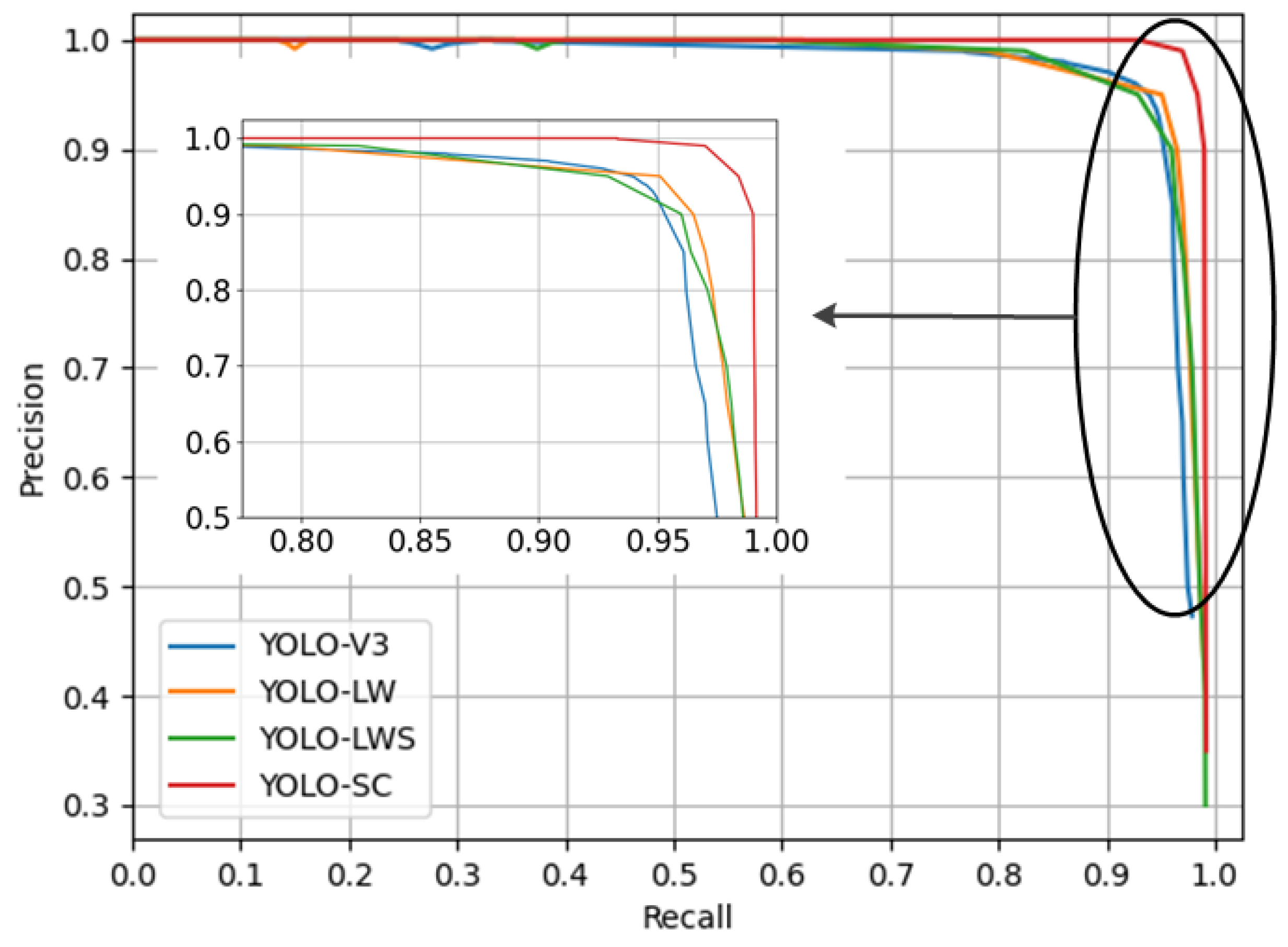
In order to verify the effectiveness of the improvement of the prototype network YOLO-V3, this paper ablates the skip connection, the lightweighted network, and the multi-structured multi-size feature fusion. The lightweight-only network is called YOLO-LW; the model with skip connections added to its base is called YOLO-LWS; and, finally, the model with multi-structured multi-size feature fusion is called YOLO-SC. The precision–recall curves (P-R curves) for the above models are shown in Figure 16. The average precision, F1 score, and detection speed for each of the above models are shown in Table 8.
According to the experimental results, it can be seen that, as the three modules are added to the YOLO-V3 model in turn, the detection accuracy of the YOLO-SC model proposed in this paper is also incremented one step at a time. When the last module is added, the overall detection accuracy of the model improves substantially, with its AP reaching 99.41%. The F1 score drops when the second module is added, but the score is not significantly different from that of YOLO-V3. The average time for model detection decreases and then increases. The decrease is due to the fact that the first module reduces one branch of the prediction network of the YOLO-V3 model, shortening the model detection process. The latter two modules enhance the extraction of position and feature information, making the model structure richer and therefore increasing the average time of detection. Overall, the average detection time of the YOLO-SC model proposed in this paper increases by 0.036 s compared to YOLO-V3. As the underwater vehicle is operating, its speed is basically maintained at a low cruising speed. During the real-time detection, YOLO-SC only needs to provide at least one detection result within 1 s. The average detection speed of the YOLO-SC model is 0.452 s. Therefore, the model can meet the requirements of real-time underwater detection.
5. Conclusions
In this study, the YOLO-SC algorithm is suggested as a solution to the issue wherein it is difficult to extract the position and feature information of the submarine cable via the prototype network of YOLO-V3 due to the blurred and blue–green underwater images. The aforementioned problems are solved by the combination of three improved modules. The lightweighted module simplifies the prediction network and shortens the detection time; the skip connection module added to the residual network enhances the extraction of position information; the multi-structured multi-size feature fusion module improves the performance of the extraction of feature information. Compared with other models that have gained application in underwater target detection, our detection model has increased the average accuracy by up to 4.2% and the F1 score by up to 22.44%, and the average time is reduced by up to 1.616 s. In conclusion, while the proposed model improves the accuracy of submarine cable recognition, it also reduces the time investment required, and thus, it can be considered a fast and high-precision inspection model.
Author Contributions
Conceptualization, Y.L. and X.Z.; methodology, Y.L.; software, Y.L.; validation, Y.L.; formal analysis, Y.L.; investigation, Y.L.; resources, Y.L.; data curation, Y.L.; writing—original draft preparation, Y.L.; writing—review and editing, Y.L. and Z.S.; visualization, Y.L.; supervision, X.Z.; project administration, Y.L. All authors have read and agreed to the published version of the manuscript.
Funding
This research was funded by Key Research and Development Program of Zhejiang Province, grant number 2021C03013.
Institutional Review Board Statement
Not applicable.
Informed Consent Statement
Not applicable.
Data Availability Statement
Not applicable.
Conflicts of Interest
The authors declare no conflict of interest.
References
- Xie, Y.; Wang, C. Vulnerability of Submarine Cable Network of Mainland China: Comparison of Vulnerability between before and after Construction of Trans-Arctic Cable System. Complex 2021, 2021, 6662232. [Google Scholar] [CrossRef]
- Aishwarya, N. Business and Environmental Perspectives of Submarine Cables in Global Market; Springer: Cham, Switzerland, 2020. [Google Scholar]
- Eleftherakis, D.; Vicen-Bueno, R. Sensors to Increase the Security of Underwater Communication Cables: A Review of Underwater Monitoring Sensors. Sensors 2020, 20, 737. [Google Scholar] [CrossRef]
- Szyrowski, T.; Sharma, S.K.; Sutton, R.; Kennedy, G.A. Developments in subsea power and telecommunication cables detection: Part 1—Visual and hydroacoustic tracking. Underw. Technol. 2013, 31, 123–132. [Google Scholar] [CrossRef]
- Chen, B.; Li, R.; Bai, W.; Li, J.; Zhou, Y.; Guo, R. Application Analysis of Autonomous Underwater Vehicle in Submarine Cable Detection Operation. In Proceedings of the 2018 International Conference on Robotics, Control and Automation Engineering, RCAE 2018, Beijing, China, 26–28 December 2018. [Google Scholar]
- Chen, B.; Li, R.; Bai, W.; Li, J.; Guo, R. Multi-DOF Motion Simulation of Underwater Robot for Submarine Cable Detection. In Proceedings of the 2019 IEEE 8th Joint International Information Technology and Artificial Intelligence Conference (ITAIC), Chongqing, China, 24–26 May 2019; pp. 691–694. [Google Scholar]
- Ding, F.; Wu, H.; Zhu, G.; Shi, Y.Q. METEOR: Measurable energy map toward the estimation of resampling rate via a convolutional neural network. IEEE Trans. Circuits Syst. Video Technol. 2020, 30, 4715–4727. [Google Scholar] [CrossRef]
- Ding, F.; Yu, K.; Gu, Z.; Li, X.; Shi, Y. Perceptual enhancement for autonomous vehicles: Restoring visually degraded images for context prediction via adversarial training. IEEE Trans. Intell. Transp. Syst. 2021, 23, 9430–9441. [Google Scholar] [CrossRef]
- Ding, F.; Zhu, G.; Li, Y.; Zhang, X.; Atrey, P.K.; Lyu, S. Anti-forensics for face swapping videos via adversarial training. IEEE Trans. Multimed. 2021, 24, 3429–3441. [Google Scholar] [CrossRef]
- Liu, L.; Ouyang, W.; Wang, X.; Fieguth, P.W.; Chen, J.; Liu, X.; Pietikäinen, M. Deep Learning for Generic Object Detection: A Survey. Int. J. Comput. Vis. 2019, 128, 261–318. [Google Scholar] [CrossRef]
- Zhao, Z.Q.; Zheng, P.; Xu, S.; Wu, X. Object Detection With Deep Learning: A Review. IEEE Trans. Neural Netw. Learn. Syst. 2019, 30, 3212–3232. [Google Scholar] [CrossRef]
- Moniruzzaman, M.; Islam, S.M.S.; Bennamounm, M.; Lavery, P.S. Deep Learning on Underwater Marine Object Detection: A Survey. In Proceedings of the International Conference on Advanced Concepts for Intelligent Vision Systems, ACIVS, Antwerp, Belgium, 18–21 September 2017. [Google Scholar]
- Qin, H.; Li, X.; Yang, Z.; Shang, M. When underwater imagery analysis meets deep learning: A solution at the age of big visual data. In Proceedings of the OCEANS 2015-MTS/IEEE Washington, Washington, DC, USA, 19–22 October 2015; IEEE: Piscataway, NJ, USA, 2015; pp. 1–5. [Google Scholar]
- Han, F.L.; Yao, J.; Zhu, H.T.; Wang, C. Underwater Image Processing and Object Detection Based on Deep CNN Method. J. Sens. 2020, 2020, 6707328. [Google Scholar] [CrossRef]
- Li, X.; Shang, M.; Qin, H.; Chen, L. Fast accurate fish detection and recognition of underwater images with Fast R-CNN. In Proceedings of the OCEANS 2015-MTS/IEEE Washington, Washington, DC, USA, 19–22 October 2015; IEEE: Piscataway, NJ, USA, 2015; pp. 1–5. [Google Scholar]
- Ren, S.; He, K.; Girshick, R.B.; Sun, J. Faster R-CNN: Towards Real-Time Object Detection with Region Proposal Networks. IEEE Trans. Pattern Anal. Mach. Intell. 2015, 39, 1137–1149. [Google Scholar] [CrossRef]
- Krizhevsky, A.; Sutskever, I.; Hinton, G.E. ImageNet classification with deep convolutional neural networks. Commun. Acm 2012, 60, 84–90. [Google Scholar] [CrossRef]
- Jalal, A.; Salman, A.; Mian, A.S.; Shortis, M.; Shafait, F. Fish detection and species classification in underwater environments using deep learning with temporal information. Ecol. Inform. 2020, 57, 101088. [Google Scholar] [CrossRef]
- Redmon, J.; Divvala, S.K.; Girshick, R.B.; Farhadi, A. You Only Look Once: Unified, Real-Time Object Detection. In Proceedings of the 2016 IEEE Conference on Computer Vision and Pattern Recognition (CVPR), Las Vegas, NV, USA, 27–30 June 2016; pp. 779–788. [Google Scholar]
- Hu, X.; Liu, Y.; Zhao, Z.; Liu, J.; Yang, X.; Sun, C.; Chen, S.; Li, B.; Zhou, C. Real-time detection of uneaten feed pellets in underwater images for aquaculture using an improved YOLO-V4 network. Comput. Electron. Agric. 2021, 185, 106135. [Google Scholar] [CrossRef]
- Bochkovskiy, A.; Wang, C.Y.; Liao, H.Y.M. YOLOv4: Optimal Speed and Accuracy of Object Detection. arXiv 2020, arXiv:2004.10934. [Google Scholar]
- Ghiasi, G.; Lin, T.Y.; Pang, R.; Le, Q.V. NAS-FPN: Learning Scalable Feature Pyramid Architecture for Object Detection. In Proceedings of the 2019 IEEE/CVF Conference on Computer Vision and Pattern Recognition (CVPR), Long Beach, CA, USA, 15–20 June 2019; pp. 7029–7038. [Google Scholar]
- Wang, K.; Liew, J.H.; Zou, Y.; Zhou, D.; Feng, J. PANet: Few-Shot Image Semantic Segmentation With Prototype Alignment. In Proceedings of the 2019 IEEE/CVF International Conference on Computer Vision (ICCV), Seoul, Korea, 27 October–2 November 2019; pp. 9196–9205. [Google Scholar]
- Fatan, M.; Daliri, M.R.; Shahri, A.M. Underwater cable detection in the images using edge classification based on texture information. Measurement 2016, 91, 309–317. [Google Scholar] [CrossRef]
- Tolstikhin, I.O.; Houlsby, N.; Kolesnikov, A.; Beyer, L.; Zhai, X.; Unterthiner, T.; Yung, J.; Keysers, D.; Uszkoreit, J.; Lucic, M.; et al. MLP-Mixer: An all-MLP Architecture for Vision. Adv. Neural Inf. Process. Syst. 2021, 34, 24261–24272. [Google Scholar]
- Joachims, T. Making large scale SVM learning practical. In Smofa A Advances in Kermal Methods Support Vector Learning; Technical Reports; Botson Ma Mit Press: Cambridge, MA, USA, 1998. [Google Scholar]
- Stamoulakatos, A.; Cardona, J.; McCaig, C.; Murray, D.; Filius, H.; Atkinson, R.C.; Bellekens, X.J.A.; Michie, W.C.; Andonovic, I.; Lazaridis, P.I.; et al. Automatic Annotation of Subsea Pipelines Using Deep Learning. Sensors 2020, 20, 674. [Google Scholar] [CrossRef]
- Balasuriya, A.; Ura, T. Vision-based underwater cable detection and following using AUVs. In Proceedings of the OCEANS ’02 MTS/IEEE, Biloxi, MI, USA, 29–31 October 2002; IEEE: Piscataway, NJ, USA, 2002; Volume 3, pp. 1582–1587. [Google Scholar]
- Chen, B.; Li, R.; Bai, W.; Zhang, X.; Li, J.; Guo, R. Research on Recognition Method of Optical Detection Image of Underwater Robot for Submarine Cable. In Proceedings of the 2019 IEEE 3rd Advanced Information Management, Communicates, Electronic and Automation Control Conference (IMCEC), Chongqing, China, 11–13 October 2019; pp. 1973–1976. [Google Scholar]
- Han, Y.; Huang, L.; Hong, Z.; Cao, S.; Zhang, Y.; Wang, J. Deep Supervised Residual Dense Network for Underwater Image Enhancement. Sensors 2021, 21, 3289. [Google Scholar] [CrossRef]
- Tang, Z.; Jiang, L.; Luo, Z. A new underwater image enhancement algorithm based on adaptive feedback and Retinex algorithm. Multim. Tools Appl. 2021, 80, 28487–28499. [Google Scholar] [CrossRef]
- Zhu, D.; Liu, Z.; Zhang, Y. Underwater image enhancement based on colour correction and fusion. IET Image Process. 2021, 15, 2591–2603. [Google Scholar] [CrossRef]
- Huang, Y.; Liu, M.; Yuan, F. Color correction and restoration based on multi-scale recursive network for underwater optical image. Signal Process. Image Commun. 2021, 93, 116174. [Google Scholar] [CrossRef]
- Redmon, J.; Farhadi, A. YOLOv3: An Incremental Improvement. arXiv 2018, arXiv:1804.02767. [Google Scholar]
- He, K.; Zhang, X.; Ren, S.; Sun, J. Deep Residual Learning for Image Recognition. In Proceedings of the 2016 IEEE Conference on Computer Vision and Pattern Recognition (CVPR), Las Vegas, NV, USA, 27–30 June 2016; pp. 770–778. [Google Scholar]
- Zhang, X.; Fang, X.; Pan, M.; Yuan, L.; Zhang, Y.; Yuan, M.; Lv, S.; Yu, H. A Marine Organism Detection Framework Based on the Joint Optimization of Image Enhancement and Object Detection. Sensors 2021, 21, 7205. [Google Scholar] [CrossRef]
- Tian, Y.; Yang, G.; Wang, Z.; Wang, H.; Li, E.; Liang, Z. Apple detection during different growth stages in orchards using the improved YOLO-V3 model. Comput. Electron. Agric. 2019, 157, 417–426. [Google Scholar] [CrossRef]
- Lam, E.Y. Combining gray world and retinex theory for automatic white balance in digital photography. In Proceedings of the Ninth International Symposium on Consumer Electronics, (ISCE 2005), Macau, China, 14–16 June 2005; pp. 134–139. [Google Scholar]
- Redmon, J.; Farhadi, A. YOLO9000: Better, Faster, Stronger. In Proceedings of the 2017 IEEE Conference on Computer Vision and Pattern Recognition (CVPR), Honolulu, HI, USA, 21–26 July 2017; pp. 6517–6525. [Google Scholar]
- Lin, T.Y.; Dollár, P.; Girshick, R.B.; He, K.; Hariharan, B.; Belongie, S.J. Feature Pyramid Networks for Object Detection. In Proceedings of the 2017 IEEE Conference on Computer Vision and Pattern Recognition (CVPR), Honolulu, HI, USA, 21–26 July 2017; pp. 936–944. [Google Scholar]
- Liu, S.; Qi, L.; Qin, H.; Shi, J.; Jia, J. Path Aggregation Network for Instance Segmentation. In Proceedings of the 2018 IEEE/CVF Conference on Computer Vision and Pattern Recognition, Salt Lake City, UT, USA, 18–22 June 2018; pp. 8759–8768. [Google Scholar]
- Liu, W.; Anguelov, D.; Erhan, D.; Szegedy, C.; Reed, S.E.; Fu, C.Y.; Berg, A.C. SSD: Single Shot MultiBox Detector. In European Conference on Computer Vision, Proceedings of the 14th European Conference, Amsterdam, The Netherlands, 11–14 October 2016; Springer: Cham, Switzerland, 2016. [Google Scholar]
Figure 1.
Partial sample brightness transformation: (a) original image, (b) brightness transformation.
Figure 1.
Partial sample brightness transformation: (a) original image, (b) brightness transformation.

Figure 2.
Example of the sample colour balance: (a) original image, (b) colour balance.

Figure 3.
Part of the sample rotated clockwise: (a) original image, (b) rotation.

Figure 4.
YOLO-V3 network structure.

Figure 5.
Proposed YOLO-SC network structure.

Figure 6.
YOLO-SC network parameters.

Figure 7.
Skip connection network parameters.

Figure 8.
YOLO-V3 predictive network structure.

Figure 9.
YOLO-SC prediction network structure.

Figure 10.
Multi-scale feature fusion of multiple structures.

Figure 11.
Sample of submarine cable dataset under different disturbances: (a) motion blur, (b) partial absence, (c) occlusion, (d) absorption and scattering effects of water on light.
Figure 11.
Sample of submarine cable dataset under different disturbances: (a) motion blur, (b) partial absence, (c) occlusion, (d) absorption and scattering effects of water on light.

Figure 12.
YOLO-SC model: example of the actual measurement results.

Figure 13.
Precision–recall curves of different models.

Figure 14.
YOLO-SC model loss curves for both datasets (top right is a magnification of the circled portion below).
Figure 14.
YOLO-SC model loss curves for both datasets (top right is a magnification of the circled portion below).

Figure 15.
P-R curves of the YOLO-SC model for two datasets (top left is a magnification of the circled part on the right).
Figure 15.
P-R curves of the YOLO-SC model for two datasets (top left is a magnification of the circled part on the right).

Figure 16.
P-R curves for each model in the ablation experiment (top left is a magnification of the circled part on the right).
Figure 16.
P-R curves for each model in the ablation experiment (top left is a magnification of the circled part on the right).


Table 1.
Image data enhancement.
| Original Image | Brightness | Color | Rotation | Total (Sheets) |
|---|---|---|---|---|
| 2399 | 799 | 799 | 801 | 4798 |
Table 2.
Sample distribution.
| Types | Sample | Assignment |
|---|---|---|
| Positive | True | |
| Negative | True | |
| Positive | False | |
| Negative | False |
Table 3.
Training set, validation set, and test set.
| Types | Dataset | Training Set | Validation Set | Test Set |
|---|---|---|---|---|
| Number (sheets) | 4798 | 2886 | 432 | 480 |
Table 4.
Computer hardware parameters.
| Type | Parameter |
|---|---|
| CPU | Intel i5 64-bit 2.3 GHz Quad-Core |
| RAM | 8 G |
| Graphics Card | NVIDIA GeForce GTX 960 M |
| Disk | 256 G SSD 1T HDD |
Table 5.
YOLO-SC model initialization parameters.
| Size of Image | Batch Size | Epoch | Initial Learning Rate | Momentum | Decay |
|---|---|---|---|---|---|
| 8 | 100 | 0.001 | 0.9 | 0.0005 |
Table 6.
Detection accuracy, F1 score, and detection speed of different models.
| Model | AP (%) | F1 Score (%) | Average Time (s) |
|---|---|---|---|
| SSD | 95.21 | 88.41 | 0.257 |
| YOLO-V3 | 95.63 | 93.79 | 0.416 |
| Faster-RCNN | 96.10 | 75.05 | 2.068 |
| YOLO-SC | 99.41 | 97.49 | 0.452 |
Table 7.
Average accuracy (AP) and F1 scores of the YOLO-SC model corresponding to the two datasets.
Table 7.
Average accuracy (AP) and F1 scores of the YOLO-SC model corresponding to the two datasets.
| Model | AP (%) | F1 Score (%) |
|---|---|---|
| Original dataset | 98.14 | 95.79 |
| Enhanced dataset | 98.95 | 96.92 |
Table 8.
Results of ablation studies with different variations. The “✓” indicates that the corresponding sub-module has been added to the framework.
Table 8.
Results of ablation studies with different variations. The “✓” indicates that the corresponding sub-module has been added to the framework.
| Model | Lightweight | Lightweight Skip | Multi-Structures | AP (%) | F1 Score (%) | Average Time (s) |
|---|---|---|---|---|---|---|
| YOLO-V3 | 95.63 | 93.79 | 0.416 | |||
| YOLO-LW | ✓ | 96.83 | 94.92 | 0.387 | ||
| YOLO-LWS | ✓ | ✓ | 96.93 | 93.53 | 0.428 | |
| YOLO-SC | ✓ | ✓ | ✓ | 99.41 | 97.49 | 0.452 |
Publisher’s Note: MDPI stays neutral with regard to jurisdictional claims in published maps and institutional affiliations. |
© 2022 by the authors. Licensee MDPI, Basel, Switzerland. This article is an open access article distributed under the terms and conditions of the Creative Commons Attribution (CC BY) license (https://creativecommons.org/licenses/by/4.0/).
Share and Cite
MDPI and ACS Style
Li, Y.; Zhang, X.; Shen, Z. YOLO-Submarine Cable: An Improved YOLO-V3 Network for Object Detection on Submarine Cable Images. J. Mar. Sci. Eng. 2022, 10, 1143. https://doi.org/10.3390/jmse10081143
AMA Style
Li Y, Zhang X, Shen Z. YOLO-Submarine Cable: An Improved YOLO-V3 Network for Object Detection on Submarine Cable Images. Journal of Marine Science and Engineering. 2022; 10(8):1143. https://doi.org/10.3390/jmse10081143
Chicago/Turabian StyleLi, Yue, Xueting Zhang, and Zhangyi Shen. 2022. "YOLO-Submarine Cable: An Improved YOLO-V3 Network for Object Detection on Submarine Cable Images" Journal of Marine Science and Engineering 10, no. 8: 1143. https://doi.org/10.3390/jmse10081143
Note that from the first issue of 2016, this journal uses article numbers instead of page numbers. See further details here.