Structural Optimization of a Muffler for a Marine Pumping System Based on Numerical Calculation


1
Research Center of Fluid Machinery Engineering and Technology, Jiangsu University, Zhenjiang 212013, China
2
Wuhan Second Ship Design and Research Institute, Wuhan 430060, China
*
Author to whom correspondence should be addressed.
J. Mar. Sci. Eng. 2022, 10(7), 937; https://doi.org/10.3390/jmse10070937
Submission received: 11 June 2022
/
Revised: 29 June 2022
/
Accepted: 6 July 2022
/
Published: 8 July 2022
(This article belongs to the Section Ocean Engineering)
Abstract
:In order to eliminate the noise in the pumping system and prolong the service life of the equipment, an optimization design method for a muffler structure is proposed. The inside of the muffler is designed with a water guide cone which plays the role of diverting the fluid in the pipeline. The muffler shell, the wall surface of the water guide cone, and the circular bottom plate adopt a porous structure. In order to achieve the best sound suppression effect of the muffler structure, the effects of different channel expansion angles and the flow area on the performance of muffler are studied the results show that when the flow channel expansion angle of the muffler is 145° and the flow area ratio is 3 times, the noise elimination performance of the muffler is the best. The structural optimization of the muffler studied in this paper is of great significance to noise reduction in the pumping system.
1. Introduction
The pump line system is widely used in marine engineering, the ship industry and other fields. The system is mainly used to transfer the mass flow, momentum flow and energy flow of fluid. Under the action of internal and external excitation, the pumping system can produce pressure pulsation in the fluid and the structural vibration of the piping system itself. This can eventually lead to damage and the noise pollution of the pumping system. This can also affect the stealth performance of the ship. Therefore, it is of great importance to propose a muffler for vibration and noise reduction in the pumping system [1,2,3,4,5,6].
In pipeline acoustics, many researchers have conducted a lot of research on pipeline noise optimization and proposed many different types of mufflers [7,8,9]. Lyu et al. [10] designed a Helmholtz muffler for noise reduction at frequencies up to 145 Hz. However, the designed muffler has a narrow muffling bandwidth, so the muffling band of the Helmholtz muffler increases, ensuring that the resonant frequency of the muffler does not change [11]. The structural parameters of the Helmholtz muffler were optimized using the genetic algorithm and the optimized structure was simulated. The simulation results showed that the muffler’s muffling bandwidth widened from 32 Hz to 86 Hz. Shao et al. [12], with recent advances in acoustic metamaterial science, have demonstrated the possibility of using Helmholtz cavity structures for sound attenuation while reducing low-frequency noise. However, in the Helmholtz cavity structure, the muffling frequency is fixed in the conventional muffler. It is very inflexible in practical applications. To meet this challenge, they first proposed a muffler with a membrane structure and multiple Helmholtz cavities. The negative mass density was derived for different numbers of membranes by simplifying the structure to a mass-spring model. The transmission loss (TL) was calculated by simulation. The analysis results confirmed that the muffler could reduce the noise when the mass density was negative, and the muffling frequency could be adjusted by changing the number of membranes. Liu et al. [13] investigated conical-neck Helmholtz resonators with a wide acoustic attenuation band performance in the low-frequency range. In order to study its broadband acoustic attenuation mechanism, three-dimensional finite element models of different neck Helmholtz resonators were constructed separately. An acoustic performance prediction model based on the one-dimensional analytical method with acoustic length correction was constructed to calculate the transmission loss results more efficiently. Additionally, the formula for the resonant frequency was derived. Then, the prediction model and formula were verified by the finite element method and experiments, and the results showed good agreement. The acoustic attenuation characteristics of the conical-neck Helmholtz resonator were analyzed using a predictive model, and the results showed that the acoustic attenuation bandwidth in the low-frequency range was improved by increasing the neck–cone angle [14]. All the above mufflers are studied on the basis of the Helmholtz resonance muffler. Although the low-frequency muffling capacity of the Helmholtz resonance muffler is high, its muffling frequency is very selective and the muffling band is very narrow, which has certain limitations. Only at the resonant frequency is the anechoic volume large, and when it deviates from the resonant frequency the anechoic effect is not obvious. Therefore, it is difficult to adapt this type of muffler to some practical situations where the excitation frequency changes or the muffling frequency band is wide. The predicted results were successfully compared with the full-scale experimental results obtained using a four-microphone standing wave tube.
Lee et al. [15] developed a compact multi-chamber silencer which contained dissipative microperforated elements that could be used to reduce transmission noise in a flow system. Two expansion mufflers connected in series were used to create a relatively compact system that effectively attenuated sound in the range of speech interference [16]. Microperforated elements were used both to improve the acoustic performance of the silencer and to reduce the system pressure drop relative to a silencer without microperforated lining. Finite element modeling (FEM) simulations and experimental methods were used in the detailed design of the multi-chamber silencer. Zhu et al. [17] proposed a new concept of a semi-active muffler device based on H-Q tubes in order to control low-frequency noise in piping systems. The semi-active muffler device performed well in the low-frequency band (especially from 50 Hz to 150 Hz). The average noise reduction level was about 35 dB, which was much better than that of passive mufflers. Between 150 Hz and 350 Hz, the performance of semi-active mufflers was better than that of passive mufflers. Above 350 Hz, it had a worse performance compared with the passive muffler. Lee et al. [18] proposed a multi-objective topology optimization problem to maximize the transmission loss at the target frequency while minimizing the voltage drop. The objective function in the formula was the sum of the weighted transmission loss and the weighted voltage drop. The influence of the weighting factor on the optimal topology of the muffler was studied. At the same time, the transmission loss and pressure drop of the muffler were optimized. Shi et al. [19] theoretically and experimentally studied the wave propagation in a periodic array of microperforated pipe mufflers. The results showed that the periodic structure affected the performance of the microperforated muffler. The combination of the periodic structure and the micro-perforated tube muffler helped to control lower frequency noise over a wider frequency range and improved peak transmission loss around the resonant frequency where the periodic distance was different. Du et al. [20] proposed a water muffler based on a Kevlar-reinforced rubber tube and an internal noise reduction structure. This muffler was designed for optimum vibration damping and hydrodynamic noise reduction. An experimental system was established to study the acoustic performance of the proposed muffler. The function of the system was confirmed by testing the reference tube. Tests of the reference tube at different speeds showed that the effect of the flow was mainly concentrated in the frequency band below 400 Hz. At present, there are few studies on pipeline system mufflers, and exploration into the influencing factors of muffler performance and the optimization and innovation of the structure is lacking. Most mufflers have specific applications. Therefore, it is of great significance to explore a new type of muffler applied to pipeline systems.
2. Methodology
2.1. Lighthill Acoustics Theory
For the study of flow noise, the Lighthill acoustic theory is a very important theoretical base. The theory is based on the assumption that an infinite uniform static acoustic medium consists of a finite region of turbulent motion. The turbulent region does not affect other regions. The change in density is similar to the trends of sound waves. The Lighthill acoustic Equation (1) can be obtained from the simultaneous derivation of the continuity equation and the momentum equation in fluid mechanics [21]:
where is fluid density fluctuation, and are fluid density and average density, respectively. t is time; is the speed of sound; is the Hamilton operator,; is the spatial coordinates; is the Lighthill tensor, ; is the pressure pulsation amount of the flow field (it is equal to the sound pressure in the far field); is the viscous stress tensor, ; and is the unit tensor, .
At this time, the acoustic analogy method assumes that the sound source in the flow field is independent and the sound propagation is not affected by the fluid, and the acoustic wave equation of the fluid can be obtained by deducing the deformation of the N-S equation. However, the Lighthill equation is obtained under the free-space assumption. Thus, is not applicable to the case of fluid–solid boundary interactions that affect sound. Curle applied the Kirchhoff integral method to extend the Lighthill theory to the case where a stationary solid boundary exists to obtain the Lighthill–Curle equation.
2.2. FW-H Equation
If the right-hand side of Equation (1) is viewed as the source term, the equation becomes a typical acoustic fluctuation equation and its solution can be obtained by applying the well-established classical acoustic method. In 1965, Lowson further developed the theory of the case where the boundary moves in any direction. On this basis, in 1969, Ffowcs Williams and Hawkings used generalized function theory to deduce the sounding equation of the control surface for arbitrary motion in static fluid, namely, the famous FW–H equation. It is shown in Equation (2) [22]:
where is the fluctuation operator; is the Dirac function (describes the immediate position of the object surface); is the surface normal vector; is the force per unit area normal to the object acting on the fluid, ; is the Kronecher symbol; and is the fluid velocity.
3. Numerical Simulation of the Muffler
3.1. The Structure Design and Working Principle of the Muffler
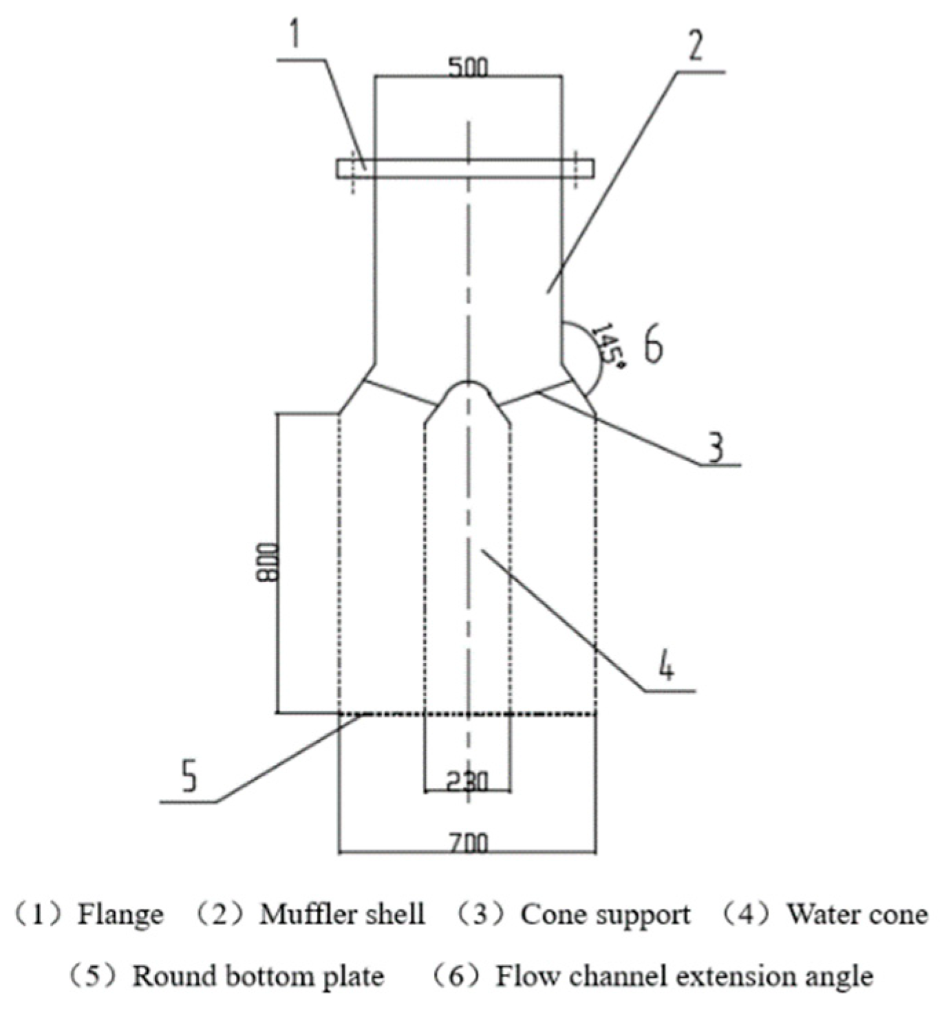
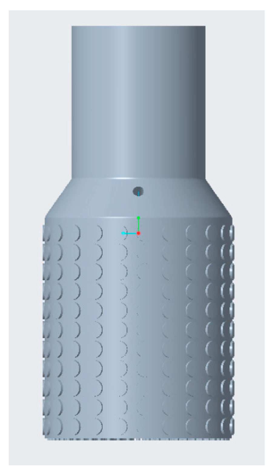
A kind of muffler used in pump pipeline systems is presented in this paper. The muffler is silenced at the outlet of the pump pipeline system. When the fluid medium flows through the muffler, the internal water guide cone divides it. The design of the water guide cone and its top arc effectively avoids the noise caused by the impact of the fluid. The muffler shell, the wall surface of the water guide cone and the circular bottom plate are uniformly arranged with a large number of microholes. The high impedance of the microhole is used to realize the muffling of the pump pipeline system. The structure and water body of the muffler are shown in Figure 1 and Figure 2.
In this paper, the noise reduction performance of the muffler is studied according to the two structural parameters of the flow channel expansion angle and the flow area ratio. The flow area is the cross-sectional area of the outlet when the fluid medium is allowed to flow out of the muffler. Therefore, this paper studies the ratio of different flow channel expansion angles and flow areas. We compare the noise reduction performance when the expansion angle of the flow channel is 120°, 145°, and 160°, and the flow area ratio is 2.5 times, 3 times, and 3.5 times.
3.2. Mesh Generation of Muffler
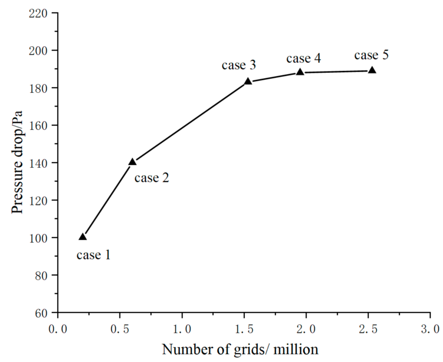
The meshing of the three-dimensional model of the muffler is based on meshing software. Considering the irregularity of the water body of the muffler, the tetrahedral mesh is used to divide the structure. The maximum size of the mesh is 0.08 m, and the maximum size of the internal acoustic net is less than 1/6 of the maximum length of the sound wave. The finer the flow field mesh is, the higher the calculation precision is. However, when the mesh is refined to a certain extent, the improvement of calculation accuracy is not obvious. Additionally, the calculation speed may be greatly reduced. The calculation speed and accuracy should be considered in mesh partitioning. The different grid schemes are shown in Table 1.
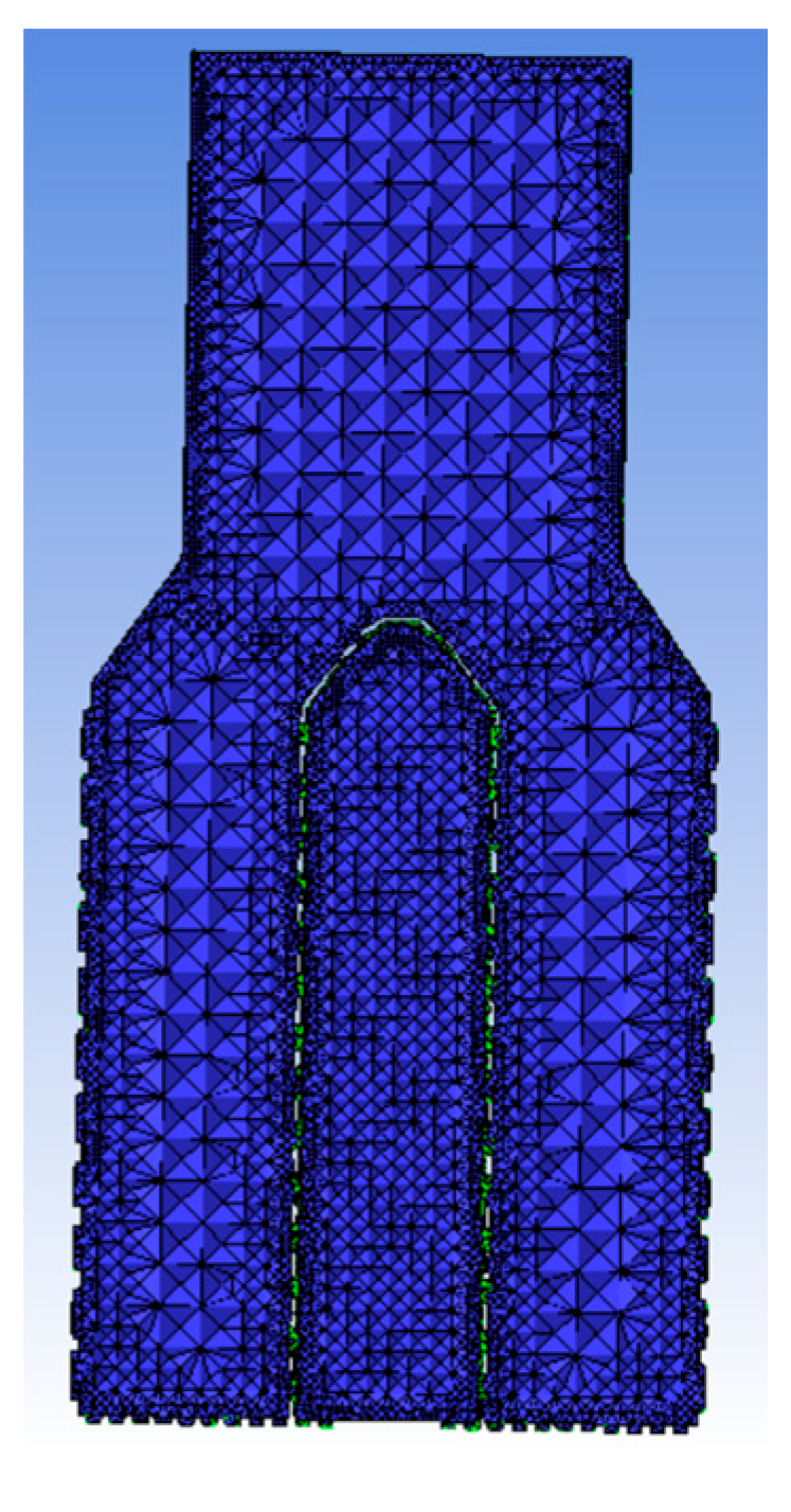
Based on the numerical results of the flow field, the pressure differences under different grid schemes are compared. As shown in Figure 3, when the mesh number reaches 1.53 million, the improvement in the computational accuracy of the mesh number is less and less obvious. Therefore, it can be considered that when the mesh number of the muffler is 1.53 million, it is most beneficial to the numerical calculation and analysis. The result of the meshing is shown in Figure 4.
3.3. Flow Field and Sound Field Numerical Simulation Settings
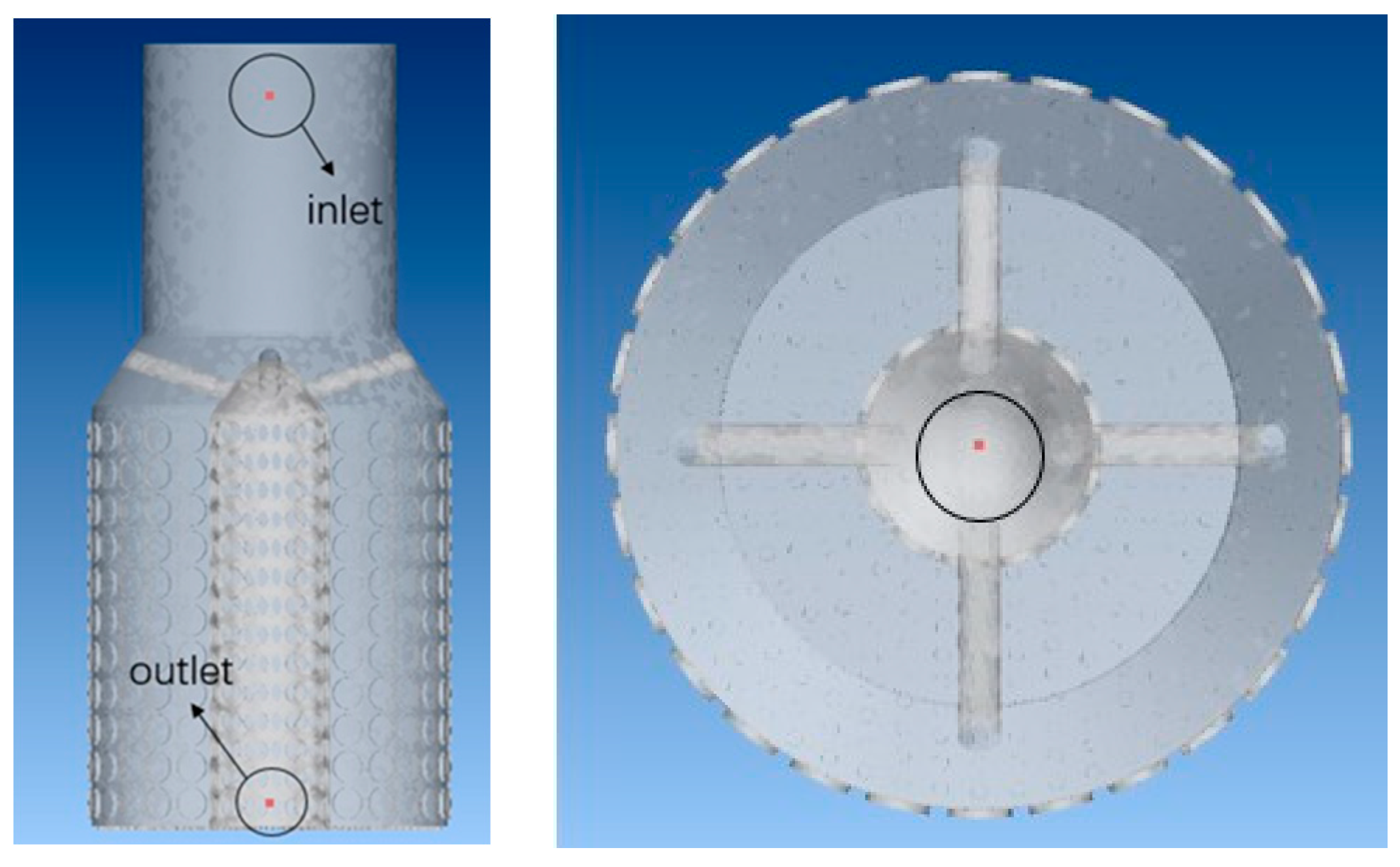
The numerical simulation of the muffler flow field is divided into two parts: steady calculation and unsteady calculation. The steady calculation is used to obtain the steady flow field and the steady flow field is taken as the initial value of the unsteady calculation. The turbulence model is used for steady-state calculation and transient calculation. The inlet and outlet boundary conditions of the muffler are the inlet velocity and outlet pressure boundary conditions, respectively. The inlet velocity is set to 0.7 m/s, the outlet pressure is set to 0.1 Mpa, the time step of the transient calculation is set to 0.000167 s, and the total time step is 0.167 s. To ensure the full development of the flow field, the time domain fluctuating pressure of the muffler needs to be taken within the stable range of the transient flow field. The sound source information of the flow field is extracted for hydrodynamic noise calculation and analysis. According to the time domain information of the sound source, the fluid-induced noise of muffler can be calculated. The sound source term in the frequency domain can be obtained by Fourier transform. When processing window functions and solving their settings, the essence of acoustic simulation is the time domain sound source through Fast Fourier Transform (FFT) to the frequency domain sound source. However, in the process of time–frequency conversion, the time–frequency energy is not completely converted to the frequency domain, which will cause spectral distortion, and the purpose of adding the window function is to reduce the signal leakage and capture the time–frequency information as completely as possible. In this example, the Hanning window with a wider main flap and a significantly smaller side flap is used to filter the low-frequency discrete streaming noise and reduce the energy leakage from the signal truncation in the time–frequency conversion and the fence effect from the FFT calculation spectrum. The Hanning window with reduced width and significantly reduced partials is used to filter the low-frequency dispersive noise. The calculated frequency range of flow-induced noise is set to 0–1000 Hz. The inlet and outlet surface groups of the muffler are defined as acoustic impedance boundary conditions. The characteristic acoustic impedance is Z = ρc = 1.5 × 10⁶ kg/(m2·s) and sound velocity is 1500 m/s. The remaining walls are assumed to be fully reflective walls. The locations of the monitoring points are shown in Figure 5 (at the inlet and outlet of the muffler).
3.4. Validation of the Numerical Model
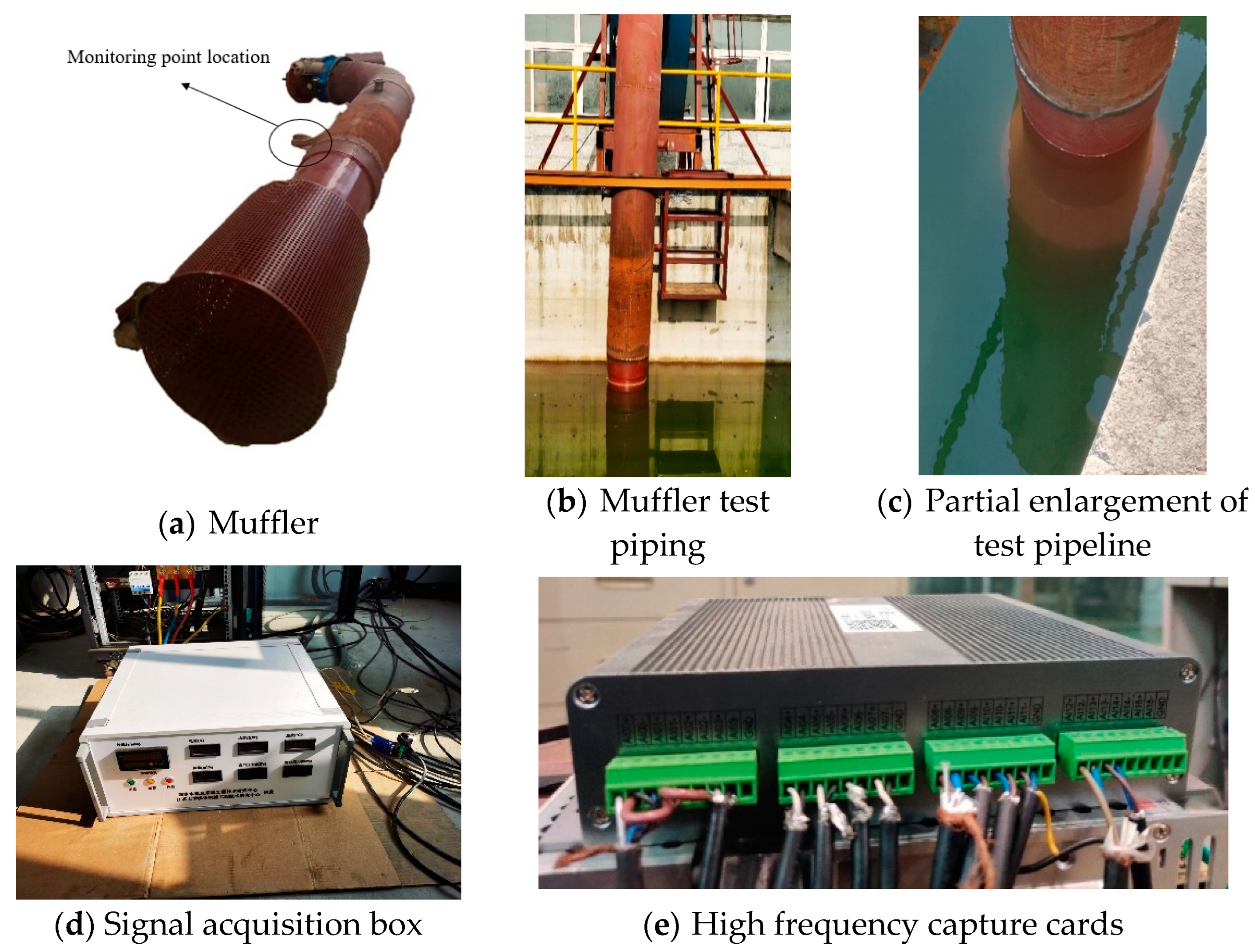
According to the muffler structure scheme obtained above, the muffler samples were manufactured and the test bench was built. The muffler sample is shown in Figure 6. It is connected to the outlet of the pumping system, installed and fixed in the pool. The pump pipeline test system is shown in Figure 6. The test device consists of a booster pump, motor, valve, pressure transmitter, flowmeter, muffler, data acquisition system, etc. Among them, the data acquisition system includes the acquisition of high-frequency signals and low-frequency signals. Hydrophones were installed at the muffler inlet and outlet positions to measure the noise. The hydrophone model was RSHA-20 with a sensitivity of 1.92 mV/Pa. When the pump was running, the output signal of the sensor was input to the virtual instrument driver through the hardware conversion of the acquisition template. The LabVIEW software was applied to realize the display and acquisition of the noise signal. The virtual instrument and the signal acquisition card are shown in Figure 6. According to the Nyquist sampling theorem, the test range of noise was used to determine the sampling interval of the acquisition module and the number of samples. Generally, the highest useful sampling frequency was 3 to 4 times. We determined the sampling frequency to be 10,240 Hz and the number of samples to be N = 30,720.
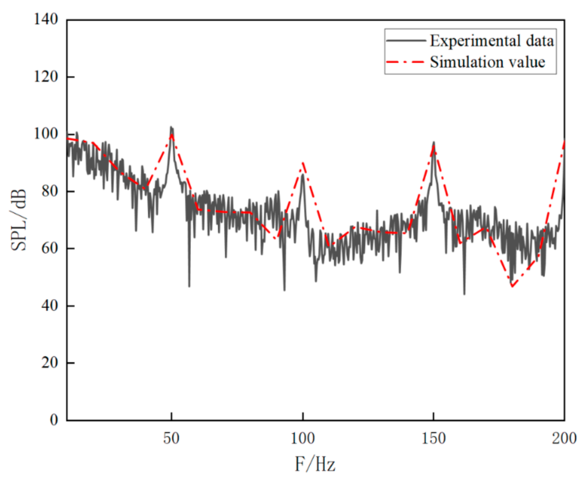
The measured data of the experiment were compared with the data of the numerical simulation, as shown in Figure 7. It can be seen from the figure that the sound spectrum obtained by the sound pressure level test of the muffler had the same trend as that of the numerical calculation. The difference in sound pressure level at the characteristic frequency was small. This proves the correctness of the numerical simulation calculation method in this paper.
4. Results and Discussions
4.1. Acoustic Cavity Modes under Different Channel Expansion Angle Schemes
The modes of the muffler cavities with different channel expansion angles were calculated by the finite element method, and the first 12 modes were selected as shown in Table 2. According to the calculation of the cavity mode, the natural frequency result and the corresponding vibration mode could be obtained. The first-order natural frequency was close to 0 Hz, which is a rigid body mode. The main reason is that the acoustic model had only a sound pressure degree of freedom, and was not constrained. According to the data analysis in the table, the natural frequencies of mufflers with different flow channel expansion angle schemes had certain differences.
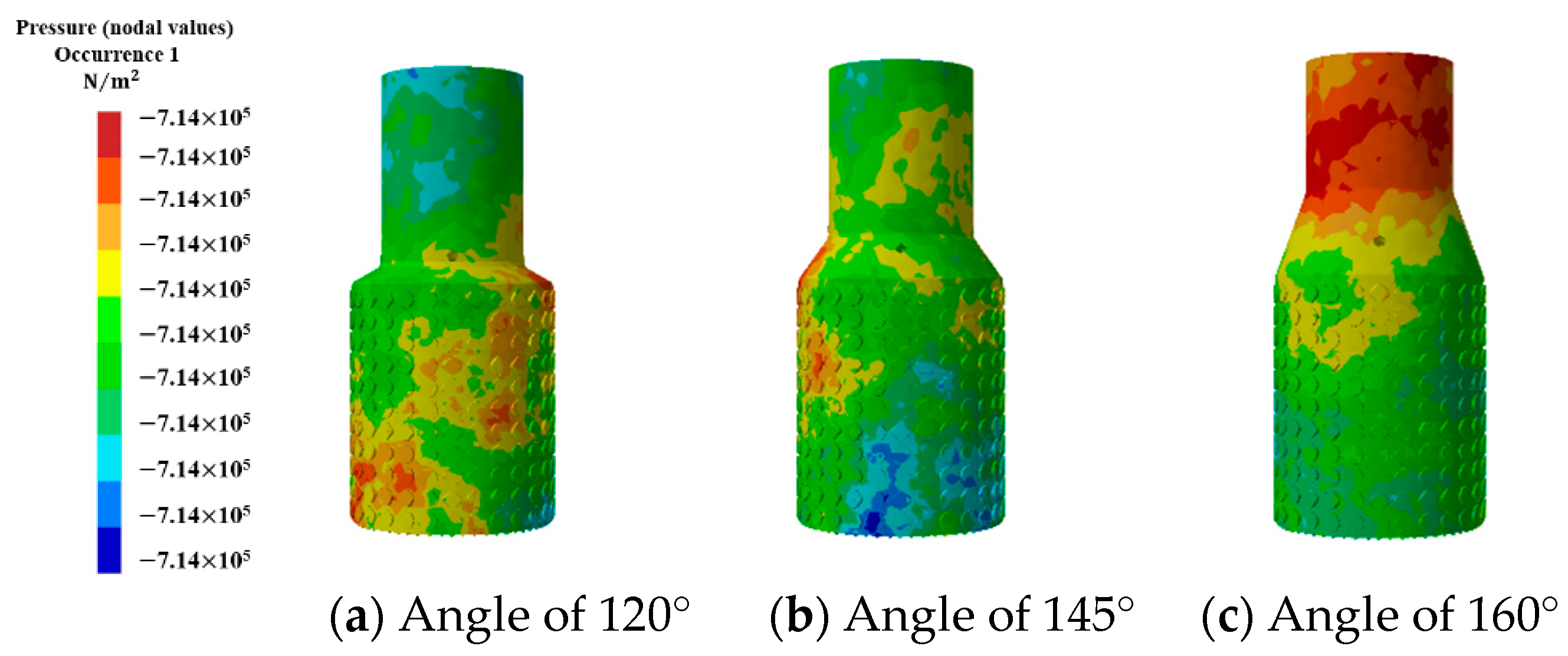
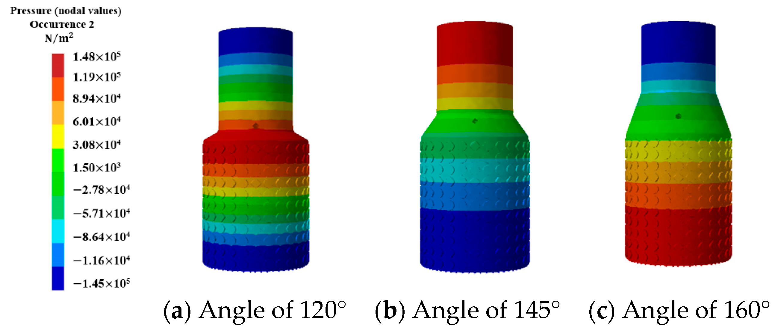
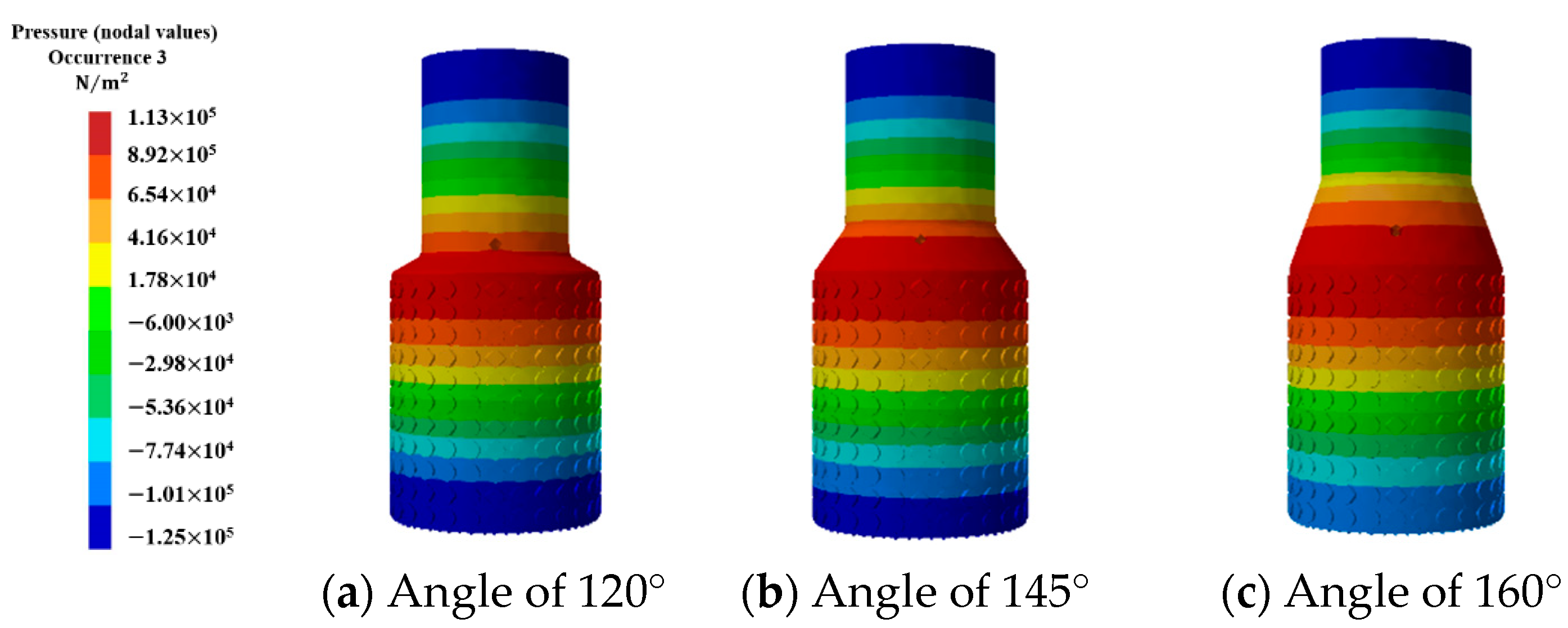
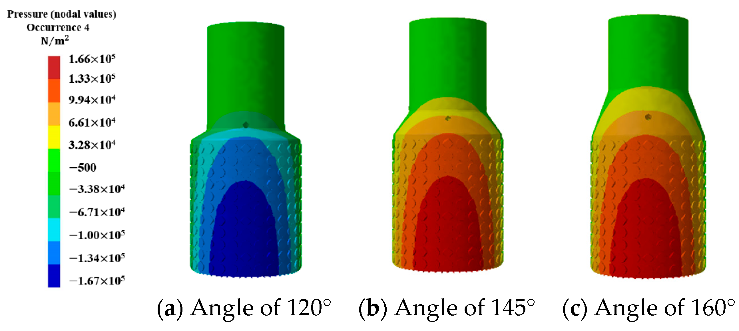
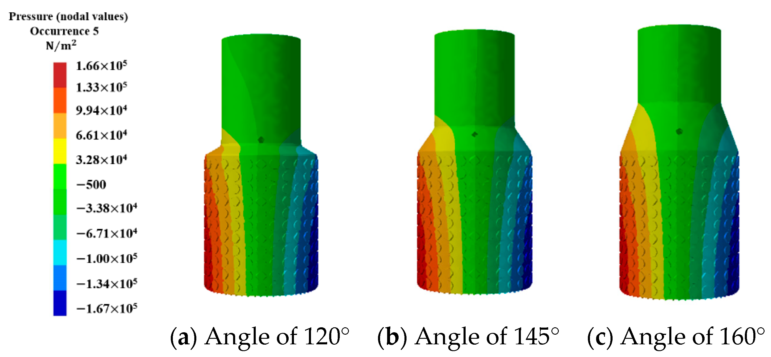
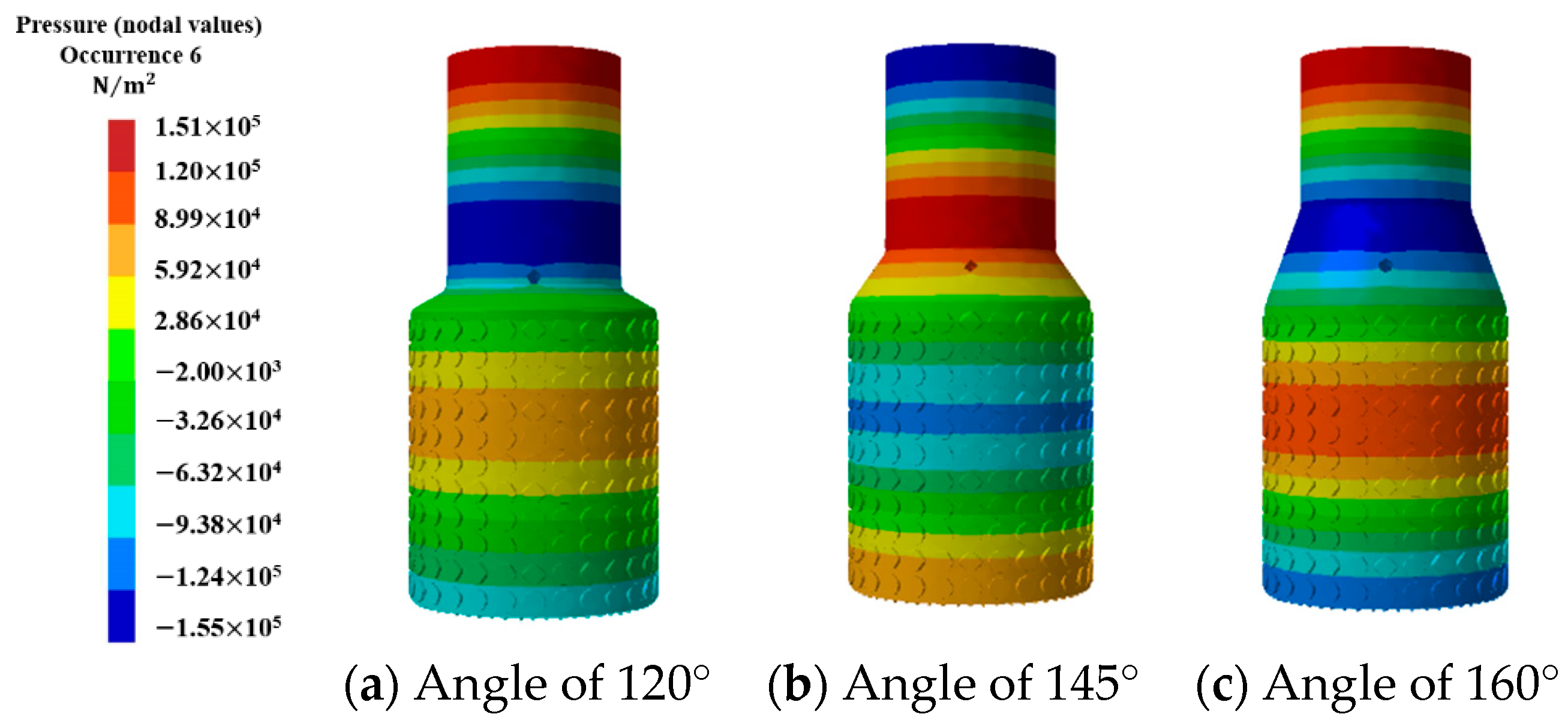
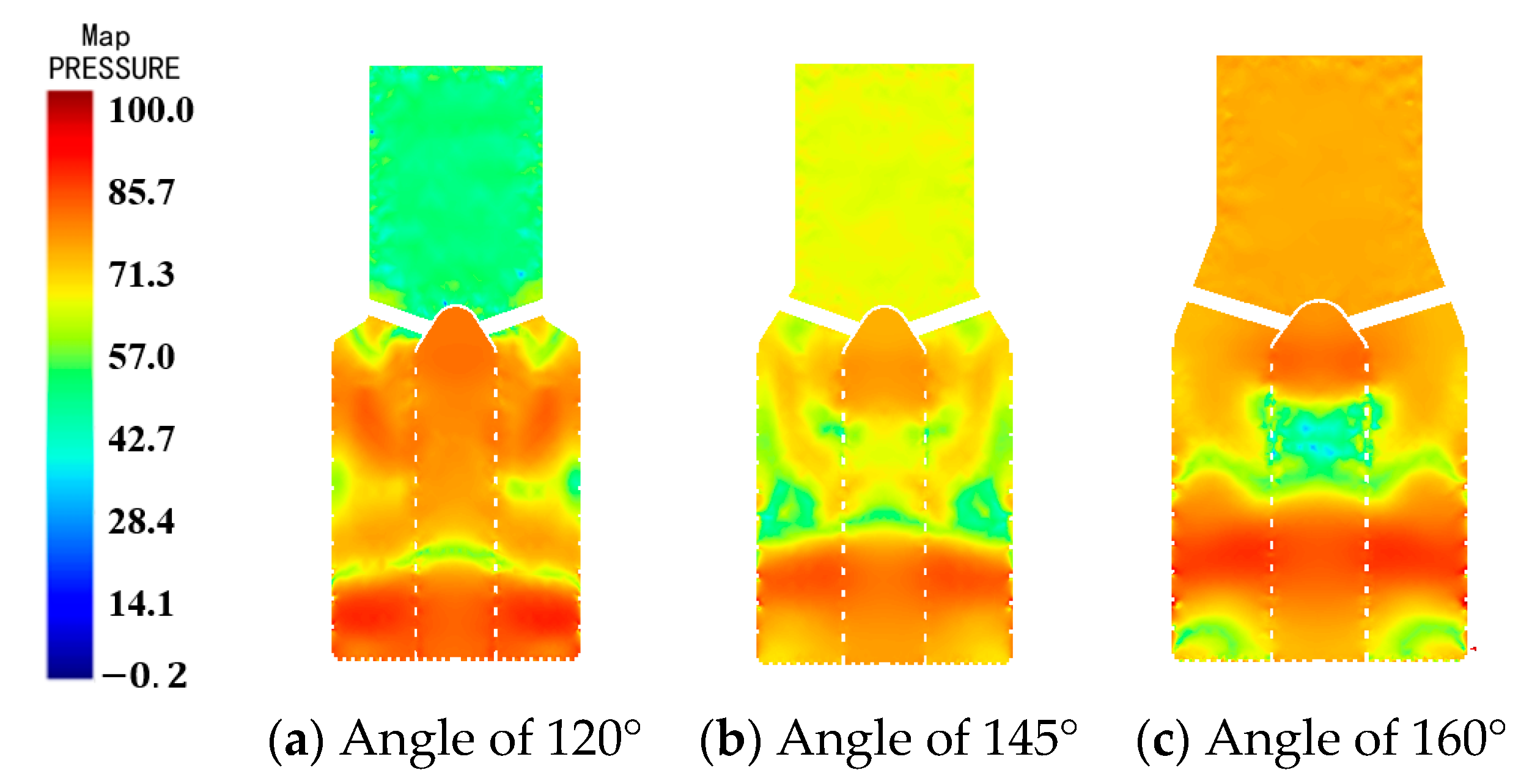
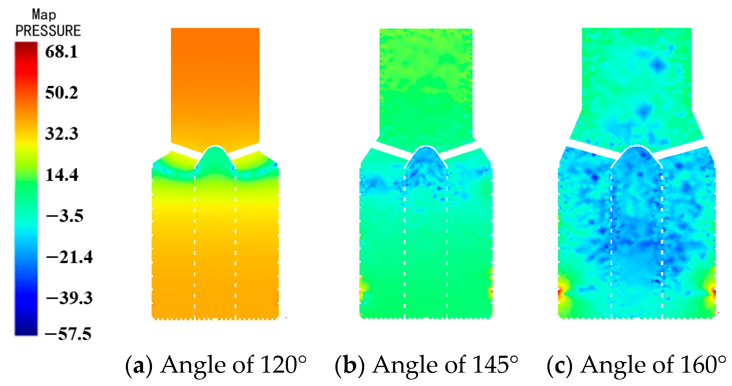
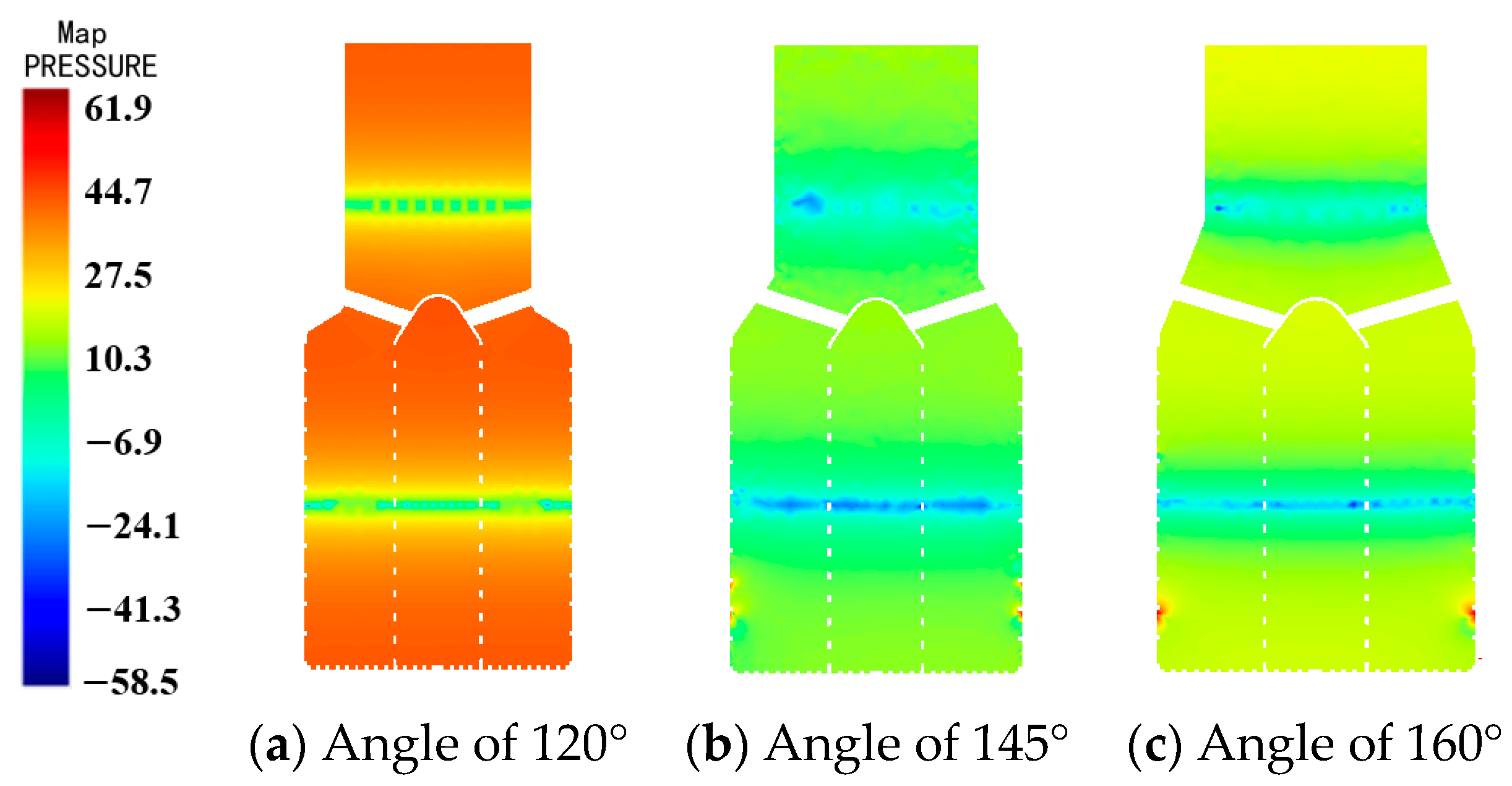
Figure 8, Figure 9, Figure 10, Figure 11, Figure 12 and Figure 13 are the first six cavity modal diagrams of different channel expansion angle schemes. According to the analysis of the results of the cavity mode, when the second-order sound pressure mode appeared, the sound pressure values of 120° and 145° decreased gradually from inlet to outlet. On the contrary, the sound pressure value of the muffler scheme with a 160° channel expansion angle gradually increased from inlet to outlet. When the third-order sound pressure mode appeared, the sound pressure value of the muffler in the middle position was larger, and the inlet and outlet were smaller. When the fourth-order sound pressure mode appeared, the sound pressure value in the middle position of the 120° scheme was the lowest. On the contrary, the middle region was in the area of high sound pressure value. When the sixth-order sound pressure mode was generated, the sound pressures at the inlet of the 120° and 160° flow channel expansion angle schemes and the middle part of the shell were larger. The muffler at 145° scheme had the opposite sound pressure distribution, and the sound pressure at the diameter change was larger.
4.2. Analysis of Numerical Simulation Results for Different Flow Channel Extension Angles
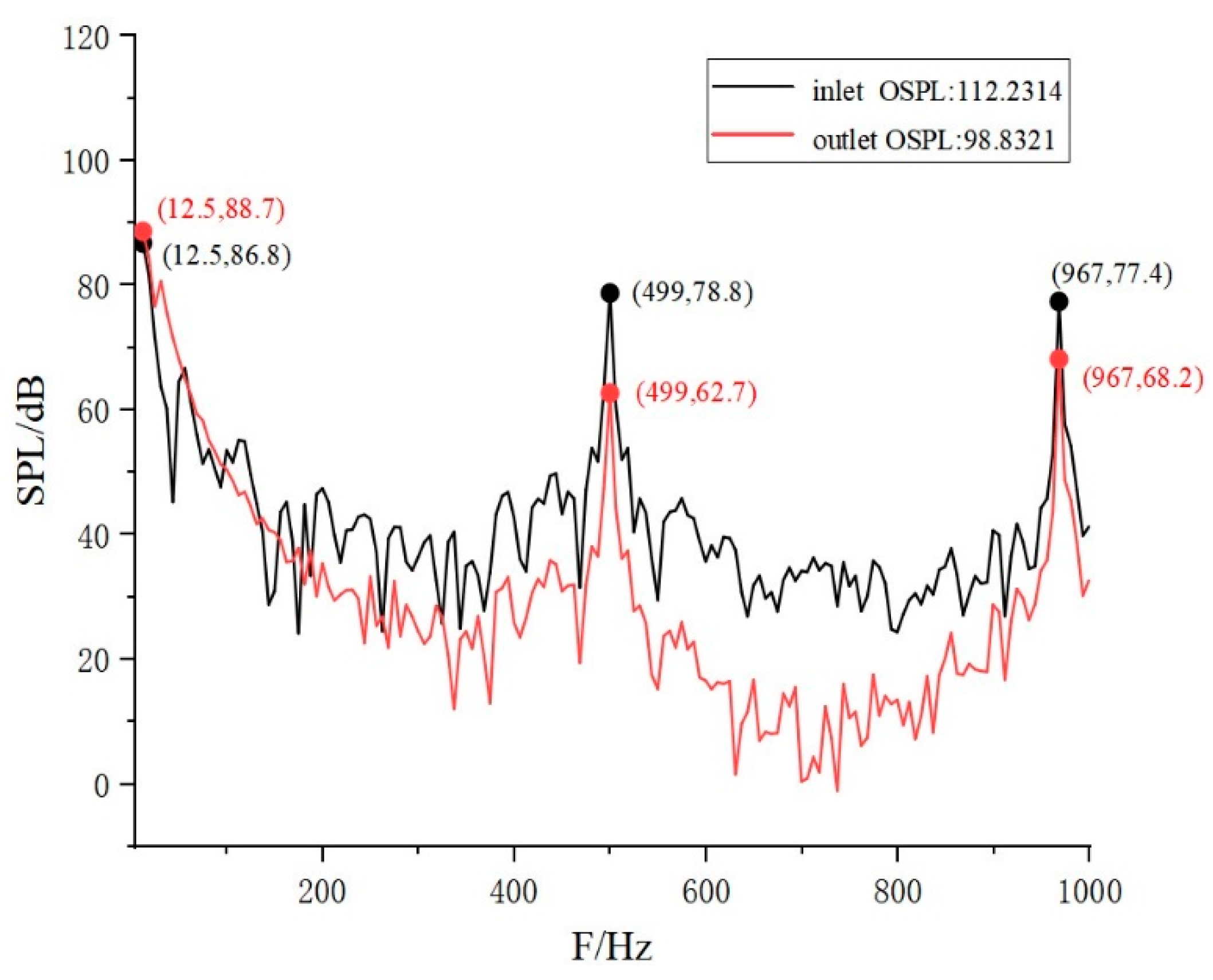
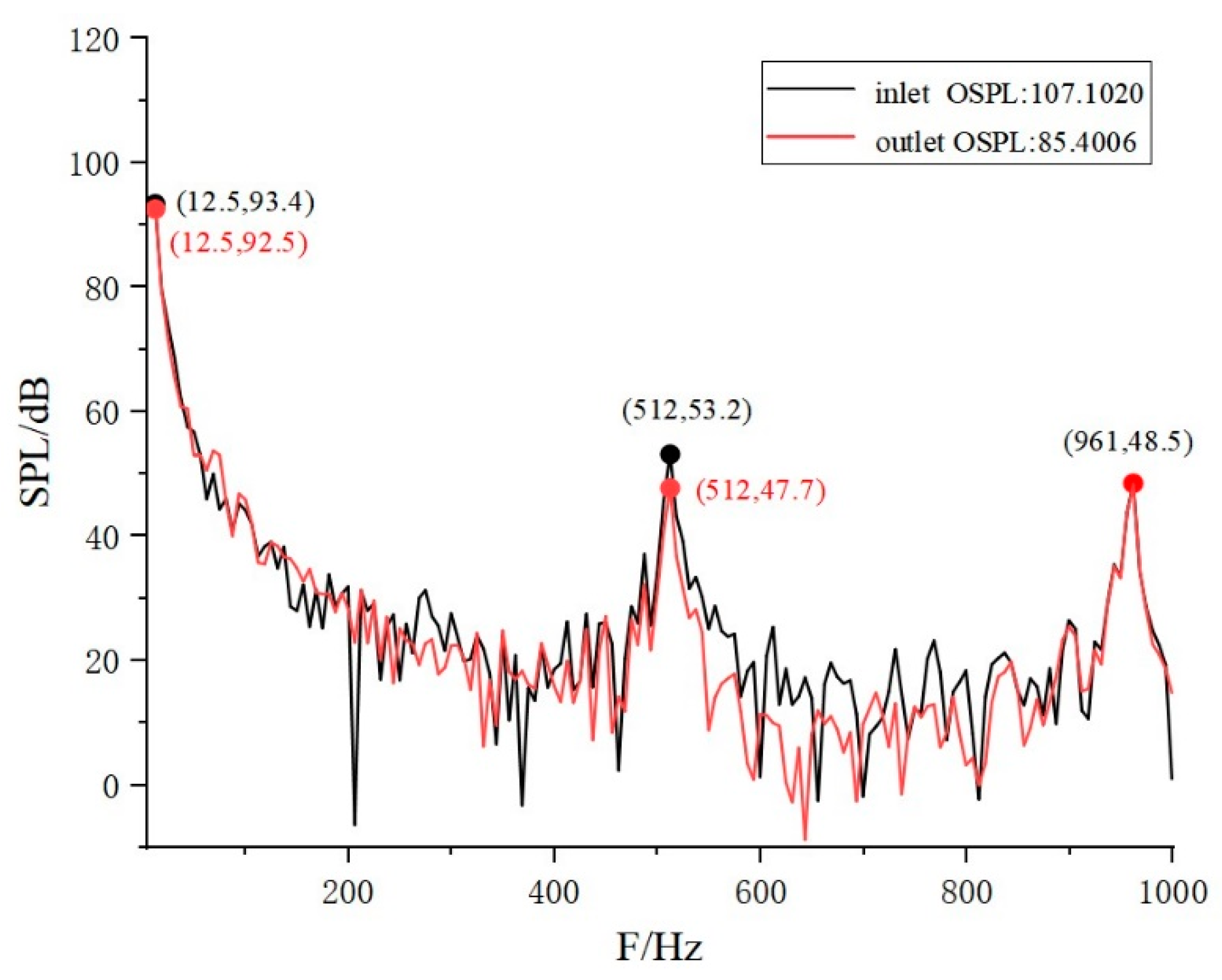
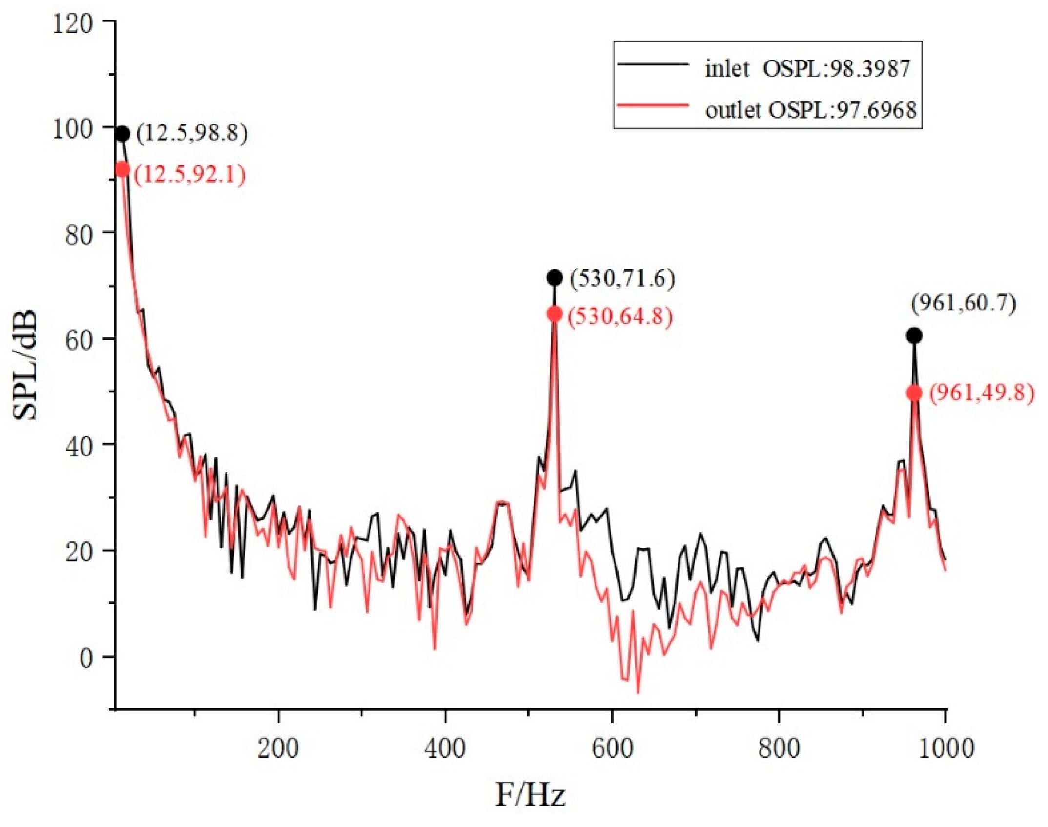
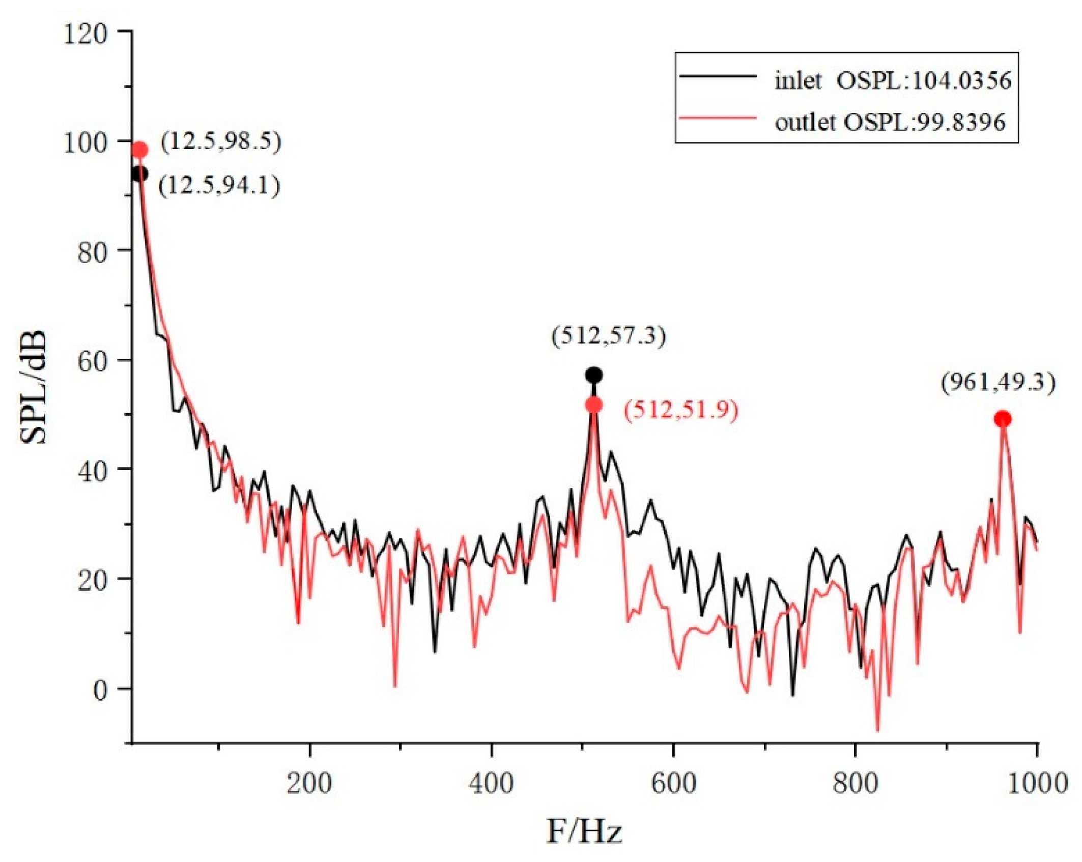
Firstly, the influence of flow channel expansion angle on muffler performance was studied. Under the condition of ensuring the same flow area of the muffler, different flow channel expansion angles were changed. Through the calculation of three different channel expansion angle schemes, the sound pressure level curves under different schemes could be obtained. The sound pressure level curves of the three schemes are shown in Figure 14, Figure 15 and Figure 16. It can be seen from the sound pressure level curve that the muffler outlet sound pressure level was less than the inlet sound pressure level. The sound pressure level curves of different schemes had the same trend. The noise was mainly concentrated at low frequencies. As the frequency increased, the sound pressure level at the entrance and exit monitoring points gradually decreased, and then fluctuated around a certain value. When the channel expansion angle was 120°, the characteristic frequencies were about 12 Hz, 499 Hz and 967 Hz. When the channel expansion angle was 145°, the characteristic frequencies were about 12 Hz, 512 Hz and 961 Hz. When the channel expansion angle was 160°, the characteristic frequencies were about 12 Hz, 530 Hz and 961 Hz. The peak value of the sound pressure level in each scheme appeared at the characteristic frequency. When the channel expansion angle was 145°, the total sound pressure level at the outlet of the muffler was about 85 dB. The total outlet sound pressure levels at 120° and 160° were about 99 dB and 98 dB, respectively. It can be seen that when the flow channel extension angle was 145°, the muffler had the best sound attenuation effect.
According to the characteristic frequencies under the different peaks, the distribution of sound pressure level was studied emphatically. As shown in Figure 17, Figure 18 and Figure 19, the distribution of sound pressure level was the most uniform when the channel expansion angle was 145°. It can be seen from the sound pressure level cloud diagram that the noise of the fluid in the pipeline significantly reduced when it passed through the muffler. The sound pressure distribution had good symmetry in the whole muffler. When the flow channel angle of the muffler was 145°, the muffler had the best performance.
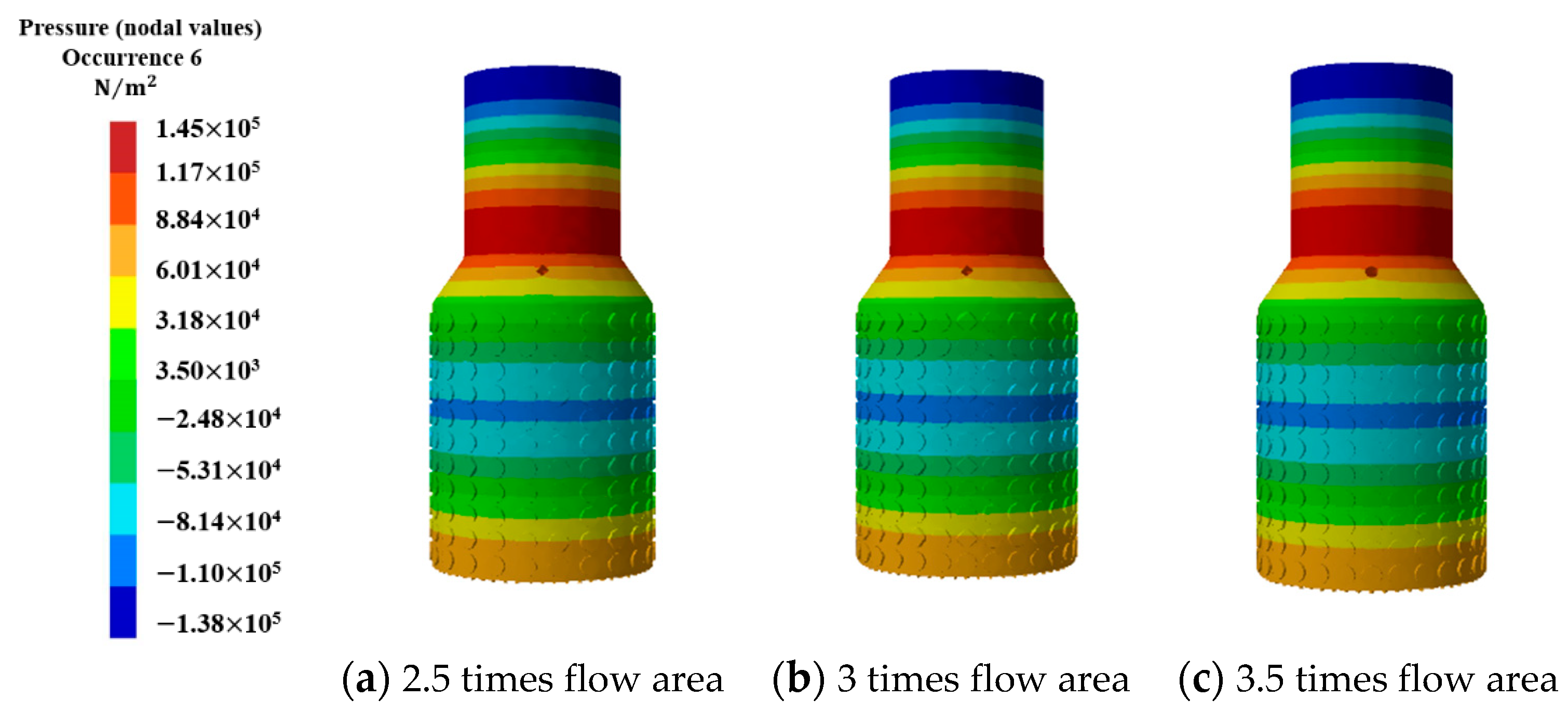
4.3. Cavity Modes under Different Flow Area Schemes
The finite element method was also used to calculate the muffler cavity modes with different flow channel extension angles. The first 12 modes are shown in Table 3. At the first order, the acoustic model had only sound pressure degrees of freedom, and the natural frequency was close to 0 Hz. According to the natural frequency analysis of different schemes in the table, it can be concluded that the change in the flow area of the muffler had little influence on the natural frequency of its cavity mode. The natural frequencies of the different schemes were almost unchanged.
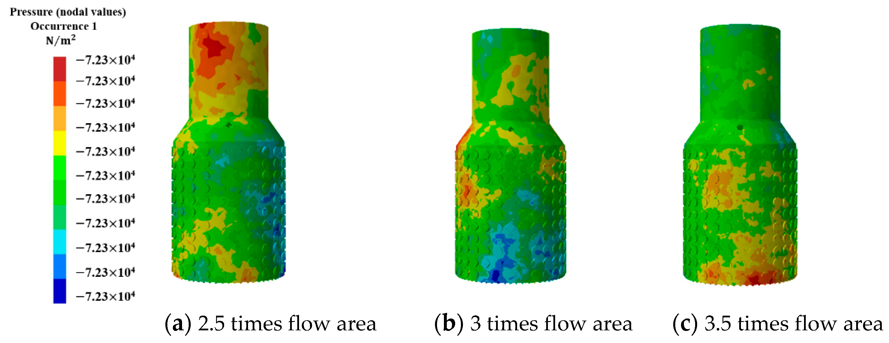
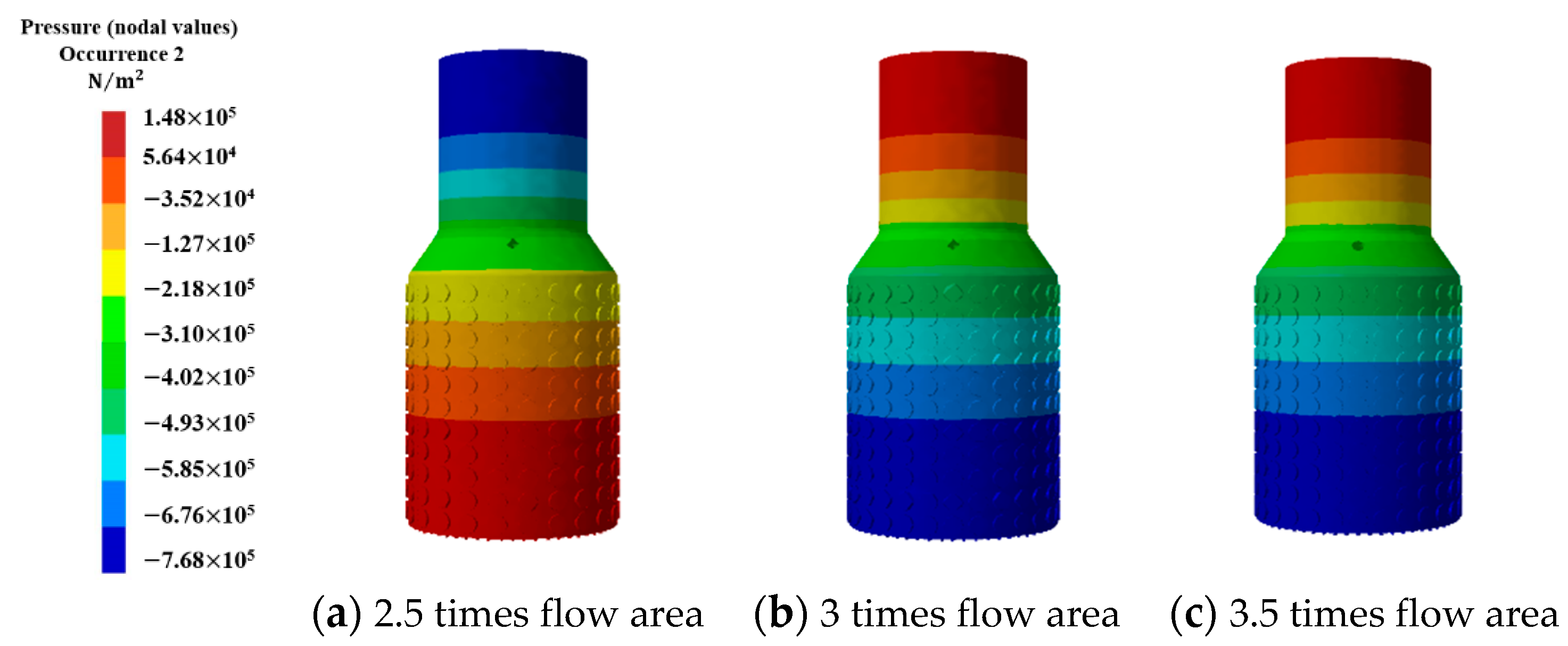
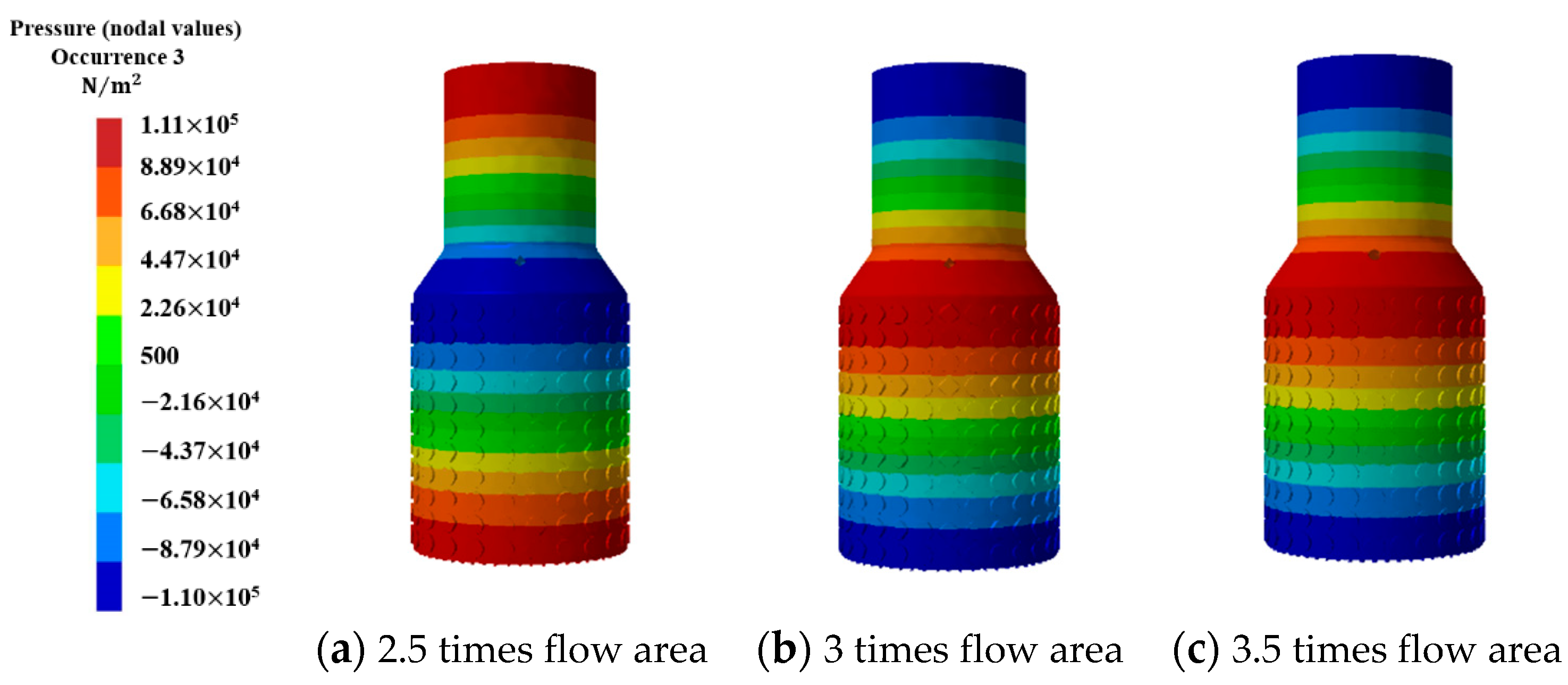
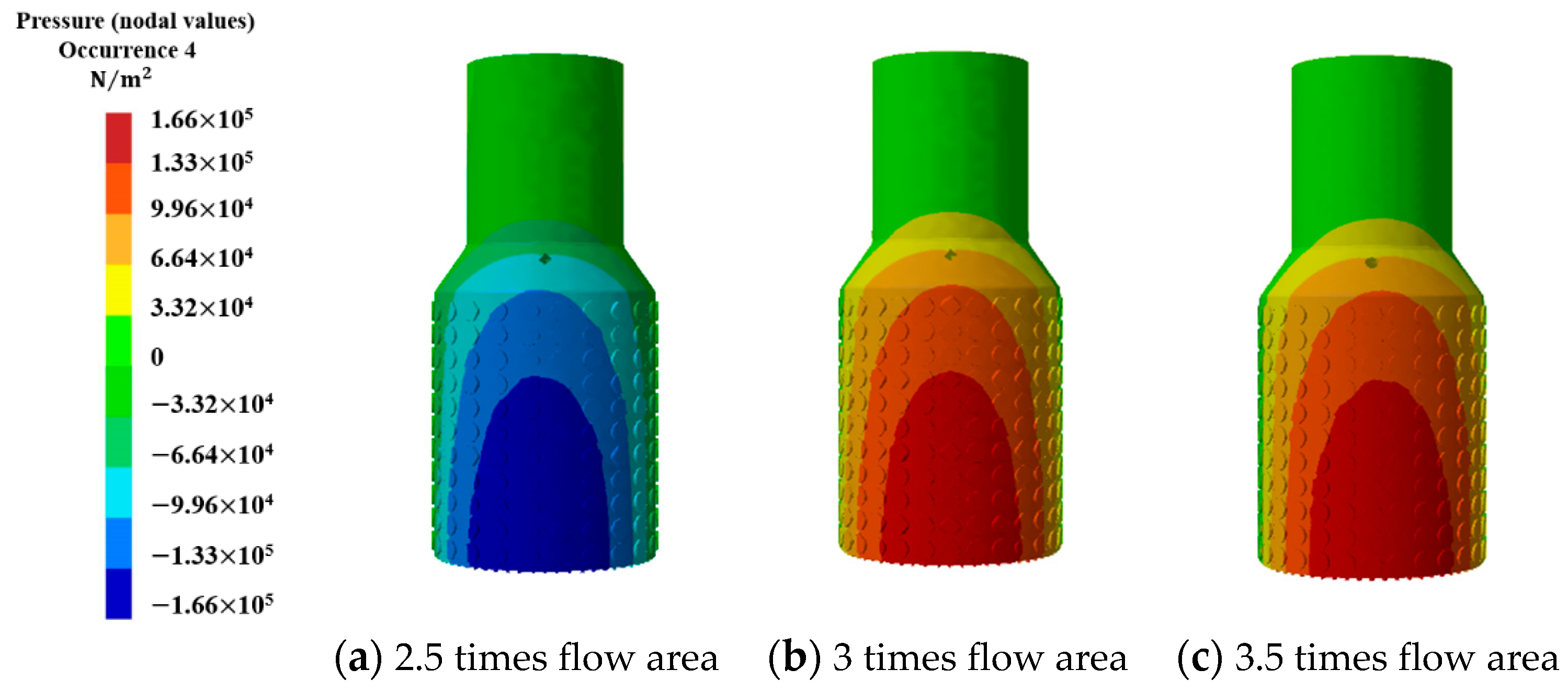
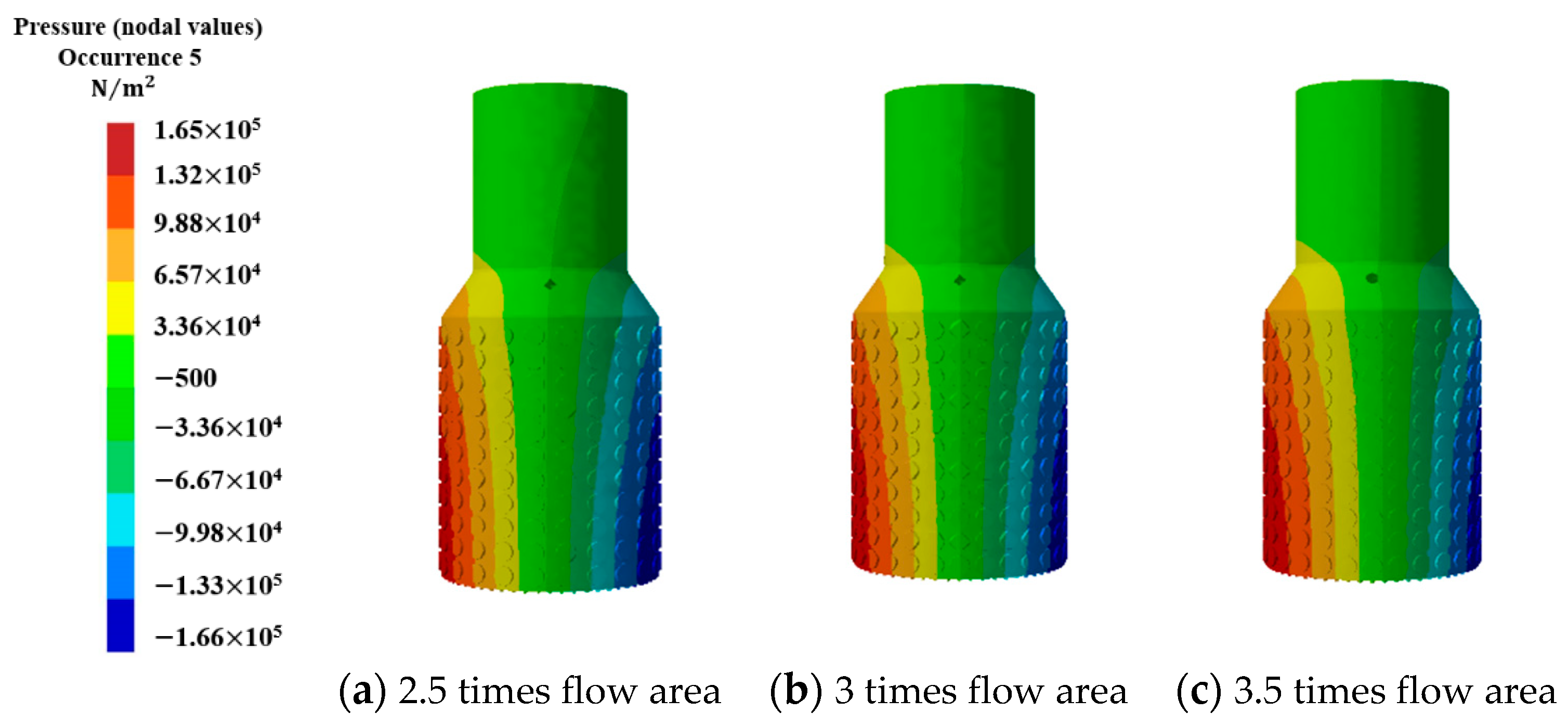
Figure 20, Figure 21, Figure 22, Figure 23, Figure 24 and Figure 25 show the cavity modal diagrams of the first six orders of different schemes with their flow areas. According to the analysis of the results of the cavity mode, when the second-order sound pressure mode appeared, the sound pressure value of 2.5 times the flow area increased gradually from the inlet to the outlet. The other two schemes gradually decreased with the inlet to the outlet. When the third-order sound pressure mode appeared, only the 2.5 times flow area scheme had higher sound pressure values at the muffler inlet and bottom outlet areas. Additionally, the middle local area was the minimum, and the 3 times and 3.5 times flow area schemes had larger sound pressure at the diameter change in the muffler. The entrance and exit positions were the smallest. When the fourth-order sound pressure mode appeared, the 2.5 times flow area scheme had a lower sound pressure value in the area near the water guide cone. The high sound pressure values of the other schemes were mainly concentrated in this area. When the sixth-order sound pressure mode was generated, the high sound pressure region of the muffler was mainly concentrated in the muffler variable diameter. Additionally, the sound pressure distribution of the muffler of different schemes was similar at this frequency.
4.4. Analysis of Noise Calculation Results for Different Flow Areas
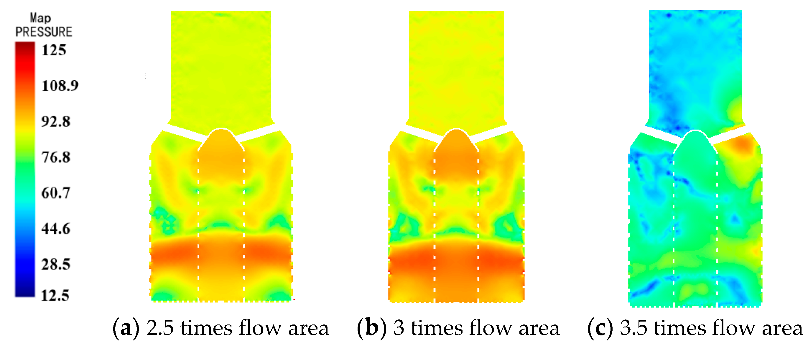
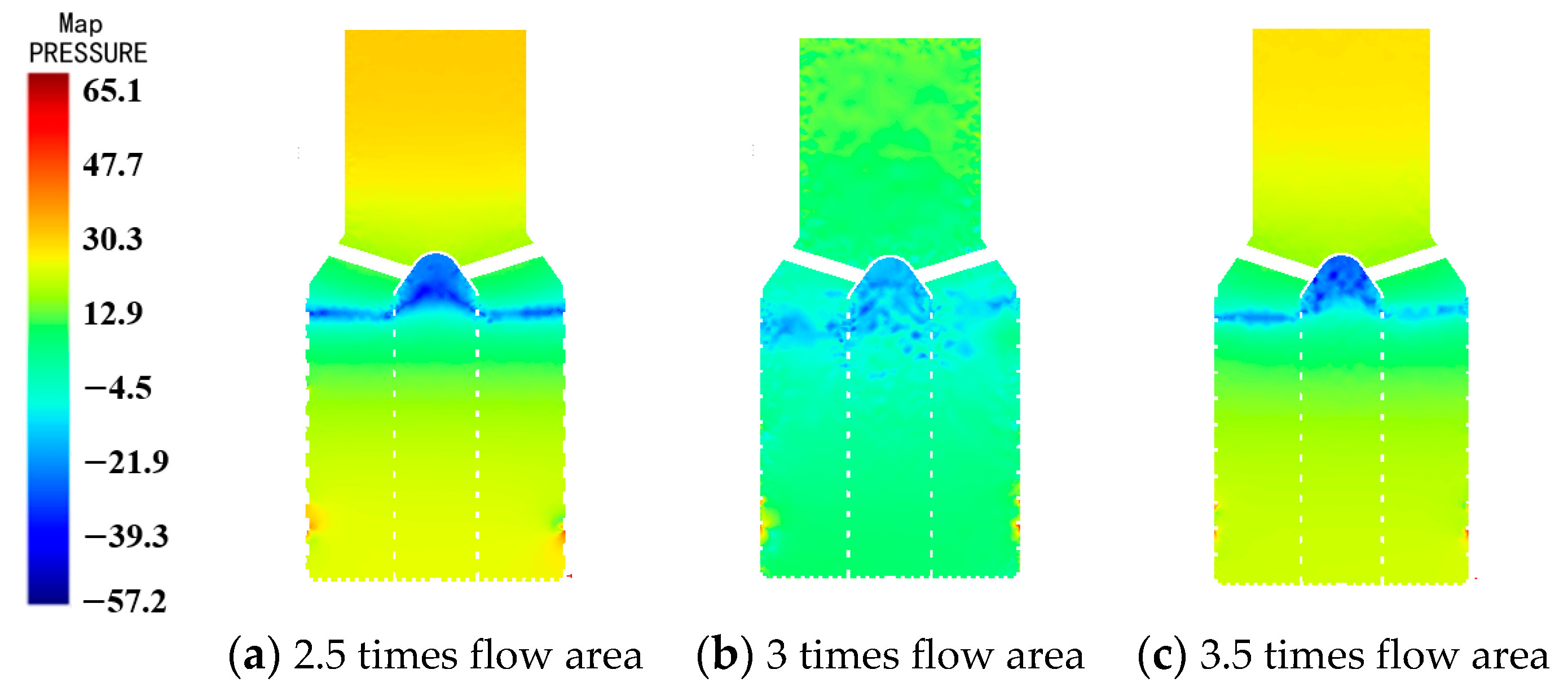
Under the same channel expansion angle, the effect of different flow area on the performance of the muffler was studied. The numerical simulations of noise with flow areas of 2.5, 3 and 3.5 times were calculated, respectively. The calculated sound pressure level curve is shown in Figure 26, Figure 27 and Figure 28. It can be seen from the figure that in the range of 0–1000 Hz, each sound pressure level graph has three characteristic frequencies corresponding to three peaks; the main characteristic frequencies are at about 12 Hz, 512 Hz, 961 Hz. The sound pressure level still gradually decreased as the frequency increased, and eventually fluctuated within a certain range. The outlet sound pressure level of the muffler under each flow area was lower than the inlet sound pressure level, which plays a role in silencing. When the flow area ratio was 3 times, the total sound pressure level of the muffler outlet was about 85 dB. When the flow area was 2.5 times and 3.5 times, the total sound pressure level was 99 dB and 91 dB, respectively. Through the comparison of the total sound pressure level, it can be inferred that when the flow area ratio was 3 times, the total sound pressure level of the muffler was smaller and the noise elimination performance was the best.
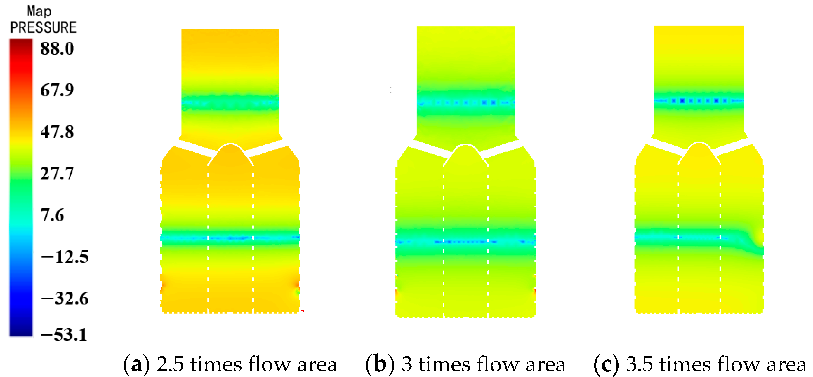
The characteristic frequency pressure distribution under different flow areas of the muffler is shown in Figure 29, Figure 30 and Figure 31. It can be seen from the figure that the sound pressure distribution law was consistent on the whole, and the higher sound pressure level was mainly concentrated in the low-frequency band. When the flow area ratio of muffler was 3 times, the distribution of sound pressure level was more uniform and the muffler had a better effect.
5. Conclusions
This article introduces a muffler structure that can be applied to a pumping system. Under the condition that the experimental results verify the feasibility of the numerical simulation method, the fluid-induced noise of the muffler can be numerically calculated. Through the analysis of numerical the simulation results, the following conclusions can be obtained:
- The general trend of the sound pressure level in the muffler was that with the increase in frequency the noise gradually decreased and finally fluctuated within a numerical range. The higher part of the sound pressure level was in the low-frequency band, and the sound pressure level at the exit monitoring point in the spectrum diagram was obviously reduced compared with the import. This shows that the muffler structure proposed in this paper has certain muffling ability. This provides a reference for the design of a muffler for a pumping system;
- In this paper, the simulation results of three channel expansion angle schemes of 120°, 145° and 160° were compared. The total sound pressure level was reduced by about 22 dB for the 145° scenario, and 13 dB and 1 dB for the 120° and 160° scenarios, respectively. The final result was that the muffler shell adopted a 145° angle to expand the cross-sectional area of the flow channel; this angle had the best effect on stable flow, vibration and noise reduction;
- In this paper, three optimization schemes with different overflow area ratios of 2.5 times, 3 times and 3.5 times were proposed. When the overflow area ratio of the muffler was 3 times, the total sound pressure level dropped by about 22 dB. Under the 2.5 times and 3.5 times schemes, the total sound pressure level dropped by about 4 dB and 11 dB. According to the comparison of different overflow area ratio schemes, when the overflow area ratio was 3 times, the fluid flow state was more stable and the anechoic capacity was better. Compared with the other solutions, the 3 times overflow area ratio was the best choice design parameter for the muffler.
Author Contributions
Supervision, investigation, H.L.; conceptualization, methodology, writing—original draft, writing—review and editing, J.L.; validation, writing—review and editing, L.D.; collating the data, R.H. All authors have read and agreed to the published version of the manuscript.
Funding
This work was supported by National Natural Science Foundation of China (No. 51879122, 51779106), Zhenjiang key research and development plan (GY2017001, GY2018025), the Open Research Subject of Key Laboratory of Fluid and Power Machinery, Ministry of Education, Xihua University (szjj2017-094, szjj2016-068), Sichuan Provincial Key Lab of Process Equipment and Control (GK201614, GK201816), Jiangsu University Young Talent training Program-Outstanding Young backbone Teacher, Program Development of Jiangsu Higher Education Institutions (PAPD), and Jiangsu top six talent summit project (GDZB-017).
Institutional Review Board Statement
Not applicable.
Informed Consent Statement
Not applicable.
Conflicts of Interest
The authors declare no conflict of interest.
References
- Wang, Z.; Chen, C.Z.; Kong, X.J. Study on Damping Measures of Pump Piping Vibration Isolation Device. Adv. Mater. Res. 2014, 971–973, 744–747. [Google Scholar] [CrossRef]
- Li, B.L.; Hodkiewicz, M.; Pan, J. A study of vibroacoustic coupling between a pump and attached water-filled pipes. J. Acoust. Soc. Am. 2007, 121, 897. [Google Scholar] [CrossRef] [PubMed]
- Gibbs, B.M.; Qi, N. Circulation pumps as structure-borne sound sources: Emission to finite pipe systems. J. Sound Vib. 2005, 284, 1099–1118. [Google Scholar] [CrossRef]
- Hayashi, I.; Kaneko, S. Pressure pulsations in piping system excited by a centrifugal turbomachinery taking the damping characteristics into consideration. J. Fluids Struct. 2014, 45, 216–234. [Google Scholar] [CrossRef]
- Wei, Z.D.; Li, B.R.; Du, J.M.; Yang, G. Research on the vibration band gaps of isolators applied to ship hydraulic pipe supports based on the theory of phononic crystals. Eur. Phys. J. Appl. Phys. 2016, 74, 10902. [Google Scholar] [CrossRef]
- Dai, C.; Zhang, Y.; Pan, Q.; Dong, L.; Liu, H.L. Study on Vibration Characteristics of Marine Centrifugal Pump Unit Excited by Different Excitation Sources. J. Mar. Sci. Eng. 2021, 9, 274. [Google Scholar] [CrossRef]
- Perrey-Debain, E.; Marechal, R.; Ville, J.M. A Special Boundary Integral Method for the Numerical Simulation of Sound Propagation in Flow Ducts Lined with Multi-Cavity Resonators. J. Comput. Acoust. 2016, 24, 1650012. [Google Scholar] [CrossRef] [Green Version]
- Shao, W.; Mechefske, C.K. Analyses of radiation impedances of finite cylindrical ducts. J. Sound Vib. 2005, 286, 363–381. [Google Scholar] [CrossRef]
- Gabard, G. Noise Sources for Duct Acoustics Simulations: Broadband Noise and Tones. AIAA J. 2014, 52, 1994–2006. [Google Scholar] [CrossRef]
- Lyu, C.M.; Lyu, H.F.; Zhang, X.G.; Wang, P.H. Optimization design of Helmholtz resonance muffler. Tech. Acoust. 2020, 39, 230–234. [Google Scholar] [CrossRef]
- Wang, X.; Mak, C.M. Acoustic performance of a duct loaded with identical resonators. J. Acoust. Soc. Am. 2012, 131, 316–322. [Google Scholar] [CrossRef]
- Shao, H.B.; He, H.; Chen, Y.; Tan, X.; Chen, G.P. A tunable metamaterial muffler with a membrane structure based on Helmholtz cavities. Appl. Acoust. 2020, 157, 107022. [Google Scholar] [CrossRef]
- Liu, H.T. Acoustic performance analysis of Helmholtz resonators with conical necks and its application. Inst. Noise Control Eng. 2019, 67, 155–167. [Google Scholar] [CrossRef]
- Qiu, X.H.; Du, L.; Jing, X.D.; Sun, X.F. The Cremer concept for annular ducts for optimum sound attenuation. J. Sound Vib. 2019, 438, 383–401. [Google Scholar] [CrossRef]
- Lee, S.; Bolton, J.S.; Martinson, P.A. Design of multi-chamber cylindrical silencers with microperforated elements. Noise Control Eng. J. 2016, 64, 532–543. [Google Scholar] [CrossRef]
- Munjal, M.L. Tuning a Two-Chamber Muffler for Wide-Band Transmission Loss. Int. J. Acoust. Vib. 2020, 25, 248–253. [Google Scholar] [CrossRef]
- Zhu, Y.W.; Zhu, F.W.; Zhang, Y.S.; Wei, Q.G. The research on semi-active muffler device of controlling the exhaust pipe’s low-frequency noise. Appl. Acoust. 2017, 116, 9–13. [Google Scholar] [CrossRef]
- Lee, J.W.; Jang, G.W. Topology design of reactive mufflers for enhancing their acoustic attenuation performance and flow characteristics simultaneously. Int. J. Numer. Methods Eng. 2012, 91, 552–570. [Google Scholar] [CrossRef]
- Shi, X.F.; Mak, C.M. Sound attenuation of a periodic array of micro-perforated tube mufflers. Appl. Acoust. 2016, 115, 15–22. [Google Scholar] [CrossRef]
- Du, T.; Lee, S.Y.; Liu, J.T.; Wu, D.Z. Acoustic performance of a water muffler. Noise Control Eng. J. 2015, 63, 239–248. [Google Scholar] [CrossRef]
- Zheng, Y.; Chen, Y.J.; Mao, X.L. Pressure pulsation characteristics and its impact on flow-induced noise in mixed flow pump. Trans. Chin. Soc. Agric. Eng. 2015, 31, 67–73. [Google Scholar] [CrossRef]
- Tang, C.D.; Wang, Z.P.; Sima, Y.Z. Systematical research on the aerodynamic noise of the high-lift airfoil based on FW-H method. J. Vibroeng. 2017, 19, 4783–4798. [Google Scholar] [CrossRef] [Green Version]
Figure 1.
Structure diagram of the muffler.

Figure 2.
Muffler water body.

Figure 3.
Grid independence verification.

Figure 4.
Cross-sectional view of muffler mesh.

Figure 5.
Sound field calculation monitoring points.

Figure 6.
Muffler piping test equipment.

Figure 7.
Comparison between simulated and experimental values of imported sound pressure level.

Figure 8.
First-order acoustic cavity modality.

Figure 9.
Second-order acoustic cavity modality.

Figure 10.
Third-order acoustic cavity modality.

Figure 11.
Fourth-order acoustic cavity modality.

Figure 12.
Fifth-order acoustic cavity modality.

Figure 13.
Sixth-order acoustic cavity modality.

Figure 14.
Sound pressure level curve at 120° angle.

Figure 15.
Sound pressure level curve at 145° angle.

Figure 16.
Sound pressure level curve at 160° angle.

Figure 17.
Sound pressure level distribution of different schemes at the first peak.

Figure 18.
Sound pressure level distribution of different schemes at the second peak.

Figure 19.
Sound pressure level distribution of different schemes at the third peak.

Figure 20.
First-order acoustic cavity modality.

Figure 21.
Second-order acoustic cavity modality.

Figure 22.
Third-order acoustic cavity modality.

Figure 23.
Fourth-order acoustic cavity modality.

Figure 24.
Fifth-order acoustic cavity modality.

Figure 25.
Sixth-order acoustic cavity modality.

Figure 26.
Spectrum diagram with 2.5 times flow area.

Figure 27.
Spectrum diagram with 3 times flow area.

Figure 28.
Spectrum diagram with 3.5 times flow area.

Figure 29.
Sound pressure level distribution of different schemes at the first peak.

Figure 30.
Sound pressure level distribution of different schemes at the second peak.

Figure 31.
Sound pressure level distribution of different schemes at the third peak.


Table 1.
Different grid schemes.
| Mesh Solutions | Total Elements |
|---|---|
| 1 | 0.2 million |
| 2 | 0.6 million |
| 3 | 1.53 million |
| 4 | 1.95 million |
| 5 | 2.53 million |
Table 2.
Natural frequencies of mufflers with different angles.
| Order Time | Angle of 120° (Hz) | Angle of 145° (Hz) | Angle of 160° (Hz) |
|---|---|---|---|
| 1 | 2.981 × 10⁻⁵ | 1.792 × 10⁻⁵ | 2.438 × 10⁻⁵ |
| 2 | 501.69 | 517.012 | 533.334 |
| 3 | 971.232 | 961.936 | 962.338 |
| 4 | 1294.053 | 1294.362 | 1294.022 |
| 5 | 1295.155 | 1295.483 | 1295.077 |
| 6 | 1510.213 | 1528.724 | 1509.541 |
| 7 | 1602.23 | 1585.376 | 1563.661 |
| 8 | 1602.845 | 1585.932 | 1564.287 |
| 9 | 1888.779 | 1897.054 | 1899.909 |
| 10 | 1889.813 | 1897.692 | 1900.519 |
| 11 | 1933.152 | 1942.872 | 1981.970 |
| 12 | 2129.332 | 2130.808 | 2108.564 |
Table 3.
Modal natural frequencies of mufflers with different flow areas.
| Order | Flow Area of 2.5 Times (Hz) | Flow Area of 3 Times (Hz) | Flow Area of 3.5 Times (Hz) |
|---|---|---|---|
| 1 | 3.414 × 10⁻⁵ | 1.792 × 10⁻⁵ | 2.53 × 10⁻⁵ |
| 2 | 517.008 | 517.012 | 515.790 |
| 3 | 962.136 | 961.936 | 961.484 |
| 4 | 1296.448 | 1294.362 | 1294.642 |
| 5 | 1297.51 | 1295.483 | 1294.790 |
| 6 | 1528.78 | 1528.724 | 1526.899 |
| 7 | 1586.674 | 1585.376 | 1583.350 |
| 8 | 1587.438 | 1585.932 | 1583.561 |
| 9 | 1897.368 | 1897.054 | 1896.341 |
| 10 | 1897.99 | 1897.692 | 1896.588 |
| 11 | 1943.35 | 1942.872 | 1939.698 |
| 12 | 2133.994 | 2130.808 | 2130.077 |
Publisher’s Note: MDPI stays neutral with regard to jurisdictional claims in published maps and institutional affiliations. |
© 2022 by the authors. Licensee MDPI, Basel, Switzerland. This article is an open access article distributed under the terms and conditions of the Creative Commons Attribution (CC BY) license (https://creativecommons.org/licenses/by/4.0/).
Share and Cite
MDPI and ACS Style
Liu, H.; Lin, J.; Hua, R.; Dong, L. Structural Optimization of a Muffler for a Marine Pumping System Based on Numerical Calculation. J. Mar. Sci. Eng. 2022, 10, 937. https://doi.org/10.3390/jmse10070937
AMA Style
Liu H, Lin J, Hua R, Dong L. Structural Optimization of a Muffler for a Marine Pumping System Based on Numerical Calculation. Journal of Marine Science and Engineering. 2022; 10(7):937. https://doi.org/10.3390/jmse10070937
Chicago/Turabian StyleLiu, Houlin, Jiawei Lin, Runan Hua, and Liang Dong. 2022. "Structural Optimization of a Muffler for a Marine Pumping System Based on Numerical Calculation" Journal of Marine Science and Engineering 10, no. 7: 937. https://doi.org/10.3390/jmse10070937
Note that from the first issue of 2016, this journal uses article numbers instead of page numbers. See further details here.