
Sea Level Change in the Canary Current System during the Satellite Era
by
 , and
, and
Nerea Marrero-Betancort
*, 
Javier Marcello
,
Dionisio Rodríguez-Esparragón
and
Santiago Hernández-León
Instituto de Oceanografía y Cambio Global (IOCAG), Universidad de Las Palmas de Gran Canaria, Unidad Asociada ULPGC-CSIC, 35017 Las Palmas de Gran Canaria, Spain
*
Author to whom correspondence should be addressed.
J. Mar. Sci. Eng. 2022, 10(7), 936; https://doi.org/10.3390/jmse10070936
Submission received: 23 May 2022
/
Revised: 1 July 2022
/
Accepted: 3 July 2022
/
Published: 8 July 2022
(This article belongs to the Special Issue Satellite Monitoring of Ocean)
Abstract
:Understanding the causes of global sea level rise is considered as an important goal of climate research on a regional scale, especially around islands, owing to their vulnerability to this phenomenon. In the case of the Canary Islands, these alterations entail an increase in territorial risks. The Canary Islands span the transitional zone linking the Northwest African upwelling system and the open ocean waters of the subtropical gyre. Here, we used satellite altimeter data to perform a detailed statistical analysis of sea level anomaly from 1993 to 2019. A seasonal study was carried out at two different regions and sea level anomaly was compared with temperature variability in the area. A total rise in the sea level of around 7.94 cm was obtained for the last 27 years in both areas. Sea level anomaly was strongly influenced by sea surface temperature, as expected. In addition, we found differences between the annual cycle in the open ocean and the upwelling zone, showing different patterns in both sites. The expected increase in sea level for the year 2050 in the coastal zone of the archipelago was estimated to be 18.10 cm, affecting the coastal economy of the islands, which is strongly based on the use of beaches for tourism.
1. Introduction
The global sea level has been rising over the past century, and the rate has increased in recent decades [1]. Understanding twentieth-century global and regional sea level changes is of paramount importance because they reflect both natural and anthropogenic changes occurring in the Earth’s climate system (through changes in land-ice and ocean heat uptake). Moreover, sea level rise affects the livelihood of hundreds of millions of people in the world’s coastal regions [2,3,4], being a serious socioeconomic problem.
Sea level changes occur because of a variety of factors including ocean tides, changes in ocean circulation, and changes in atmospheric pressure, among others. However, the long-term sea level is mainly influenced by changes in the heat content of the oceans (thermal expansion) and the exchange of water between oceans and continents [2]. Currently, the rate of global mean sea level (GMSL) rise is 3.2 mm/year, mainly due to thermal expansion and the melting of Greenland, Antarctica, and mountain glaciers [3]. However, this rate is expected to accelerate in the coming decades [1,3]. The IPCC estimates GMSL could rise between 0.28 and 0.98 m during this century depending on how greenhouse gas emissions change in the future. Recent predictions indicate a sea level rise between 0.7 and 1.2 m [5] and 0.75–1.9 m [6,7] in high warming scenarios. On the other hand, assuming a rapid melt of global icesheets, as reported for past global warming periods in the Pleistocene, up to more than 6 m could be expected by the end of the century [8]. Moreover, recent satellite-based ice loss detections [9], updates of glacier retreat, ice drainage velocity in Antarctica [10], and new data on glacial valley depth and subaqueous glacier melting in Greenland [11] suggest that sea level rise projections might have to be corrected upwards. The uncertainties in these projections will depend on our ability to understand the magnitude and factors affecting this phenomenon.
As indicated, several studies reveal changes in global sea level [5,6,7,12,13,14,15,16], but very few provide those changes at the regional scale owing to a lack of data continuity. Regional sea level change could be quite different from the global mean owing to different climatic and oceanic conditions. In addition, the regional pattern of sea level change may offer clues to the cause of these changes, which is important for predicting their magnitude and regional variations in future changes.
In this sense, the Canary Current System (CCS) is part of the North Atlantic subtropical gyre and is mainly formed by two contrasting zones: an oceanic area, which is part of the North Atlantic subtropical gyre, and the coastal upwelling zone, supporting one of the most productive areas of the world [17,18]. A main feature of this oceanic boundary area is the presence of the Canarian Archipelago, forming a barrier of more than 600 km in the path of the Canary Current [19]. The archipelago consists of seven main islands zonally distributed across the eastern branch of the subtropical gyre of the North Atlantic, at a latitude near 28° N [17]. In particular, islands, archipelagos, and coastal zones are vulnerable areas to sea level change because of significant environmental, social, and economic fragility, being able to promote significant alterations as a result of climate change [20,21,22].
In this context, satellite altimeter measurements have revolutionized the field of sea level science, and thus they provide a valuable instrument for assessing the impacts of local sea level changes. In this study, we present an exhaustive analysis of sea level variability over the last 27 years in the CCS. In this study, we distinguished the two main areas, the open ocean around the Canary Islands and the coastal upwelling zone off Northwest Africa. Seasonality of temperature is rather different in these two zones owing to differences among seasons and their effect on the coastal upwelling owing to the variability in the Trade Winds promoting Ekman transport. Thus, we aimed to study the changes in the rate of sea level increase, its seasonality, and their relationship to natural and long-term variability in this area of the Atlantic Ocean. We also extended our study to the coastal zone as the economy of the archipelago is mainly based on the use of beaches for tourism.
2. Materials and Methods
We mainly used satellite altimeter data from TOPEX/Poseidon (1992), Jason-1 (2001), and Jason-2 (2008) missions, providing a record of sea level change with a 10-day temporal resolution. These missions deliver the most accurate long-term robust sea level data at global and regional scales [23,24]. The GMSL record from these missions has provided a fundamental indicator of how climate change is affecting the Earth system [3].
The monthly mean sea level anomaly (MSLA) data used in this study were produced by SSalto/Duacs and distributed by Archiving, Validation, and Interpretation of Satellite Oceanographic data (Aviso+) and Copernicus Marine Environment Monitoring Service (CMEMS) (https://www.aviso.altimetry.fr (accessed on 1 September 2021)). These products are derived from a process integrating data from several altimeter missions: Haiyang-2A, Saral/AltiKa, Cryosat-2, OSTM/Jason-2, Jason-1, Topex/Poseidon, Envisat, GFO, and ERS-1&2. The MSLA used corresponds to the global daily maps of delayed-time sea level anomalies averaged monthly from January 1993. Data are available on a Cartesian grid, with a geographical resolution of 1/4° × 1/4° ≈ 25 km × 25 km. For our study, the period between January 1993 and December 2019 was chosen, covering a total of 27 years.
On the other hand, night sea surface temperature (NSST) products are produced and distributed by the NASA Goddard Space Flight Center Ocean Data Processing System (OPDS) (https://oceancolor.gsfc.nasa.gov/ (accessed on 2 October 2021)). NSST data are standard mapped image (SMI) products that are created from the corresponding Level 3 binned products generated from Aqua sensor, installed on the MODIS satellite. Products represent a mean at each global grid point. This product is a two-dimensional array of an equidistant cylindrical (also known as Plate Carrée) projection of the globe, with a geographical resolution of 4 km.
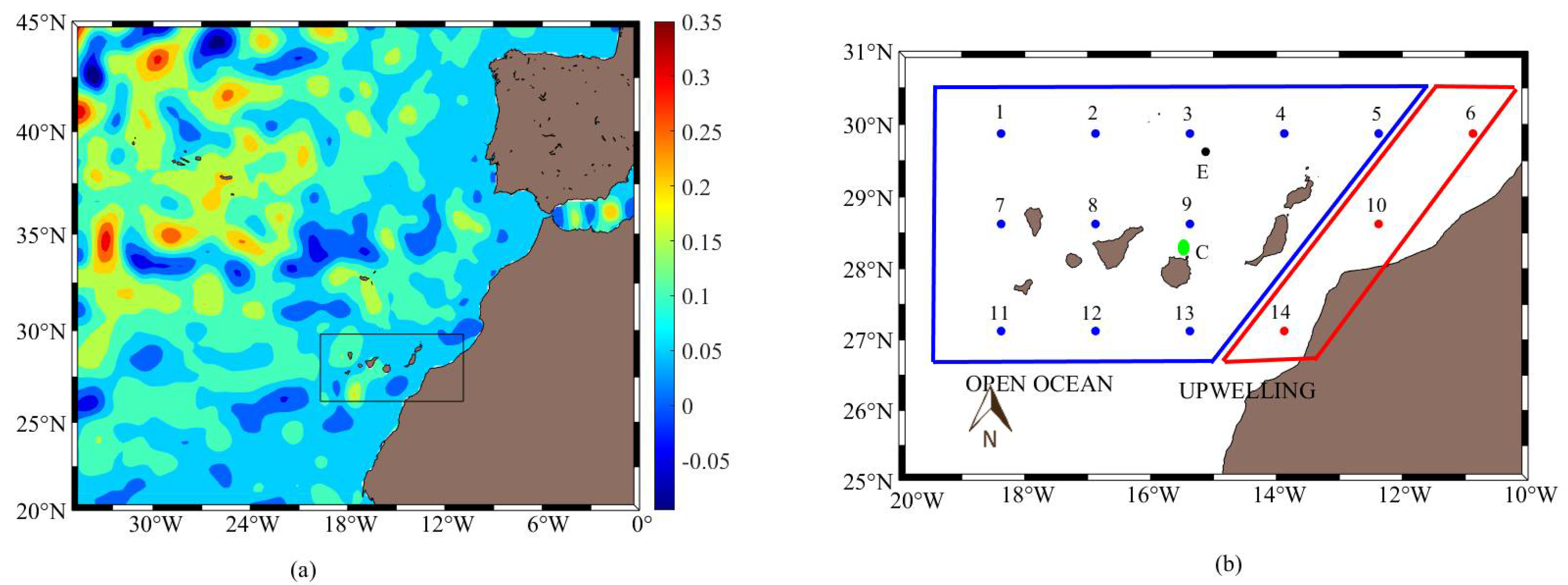
Figure 1a shows the location of the study area. From the MSLA and NSST global products, we extracted the subset of interest for this study corresponding to the area between 25° and 31° N and 10° to 20° W (Figure 1a). To carry out a detailed analysis of the complete area, we also selected a grid of 14 equidistant points, which included the Canary Archipelago and the Northwest African upwelling. Blue dots correspond to the open ocean analysis, while the red dots correspond to the upwelling area (Figure 1b). With the aim to study the relation of MSLA with different ocean parameters and global climate patterns, we selected a location to the north of the archipelago (29.52° N, 15° W; Figure 1b, black dot), away from the coast, to avoid disturbances due to island orography and because it is close to the European Station for Time-Series in the Ocean (ESTOC), north of the Canary Islands [25]. In addition, we analyzed the long-term trend in MSLA in the most important urban beach of the archipelago, located north of Gran Canaria Island (Figure 1b, green dot).
3. Results
We carried out two separate analyses to discern between the oceanic (blue dots in Figure 1b) and upwelling (red dots in Figure 1b) zones, as their oceanographic climate is rather different in both areas. Sea level values in the oceanic area of the Canary Current intensified during the last decade, showing the most remarkable anomalies in 2012 and 2017 (Figure 2).
Because of the different oceanographic scenarios observed around the Canary Islands, we discerned between the north of the islands, characterized by low mesoscale activity, the middle of the islands, and the south of them, with the latter being characterized by the presence of cyclonic and anticyclonic eddies (Table 1). We also analyzed the upwelling zone because of the sharp difference in oceanographic conditions (mainly temperature). According to Table 1, we observed the highest average values in samples located in the middle of the islands (stations 7, 8, and 9, Figure 1b). However, the maximum values were obtained in the upwelling area (stations 6, 10, and 14, Figure 1b). In contrast, the lowest values were observed in the north of the islands (stations 1, 2, 4, and 5, Figure 1b). However, regressions analyses were similar for all zones, implying that sea level rise was not statically different in all studied areas (p > 0.001, Student’s t-test). We found a total sea level variation of 7.94 cm for the entire period of study in both zones.
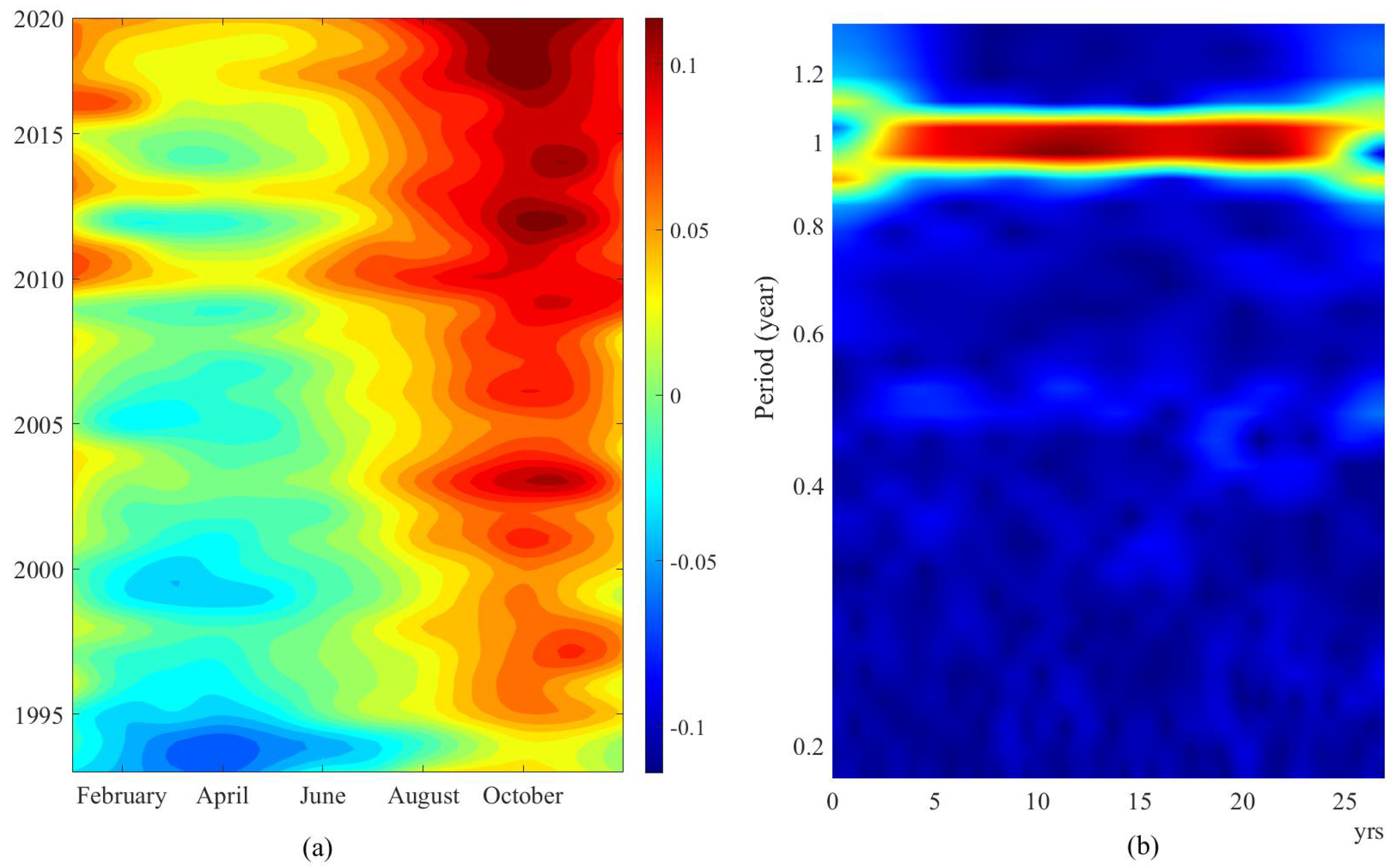
In the oceanic zone, positive anomalies were centered in autumn, reaching values up to 12 cm in October, while negative values were observed during spring (April) (Figure 2a). The positive sea level anomalies increased during the whole study period, but remarkably since 2010, encompassing summer, autumn, and winter. Negative anomalies covered the period from January to August during the 1990s (dark blue color in Figure 2a), decreasing through the study period, especially after 2010. In recent years, the negative anomalies almost disappeared. This interannual variability showed sea level height displaying an annual cycle, as clearly observed in the frequency analysis using the wavelet transforms (Figure 2b).
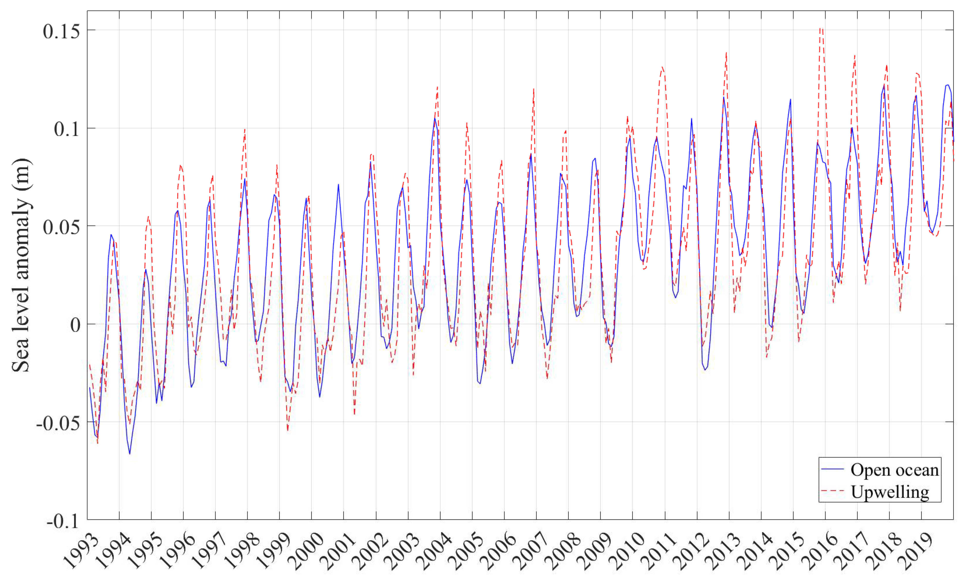
MSLA values in the time series of the upwelling region (red dashed line in Figure 3) showed higher values than in the oceanic zone (blue line). This fact is consistent because of the physical scenario of the upwelling system. Trade Winds blow parallel to the coast, promoting Ekman transport and displacing the coastal surface water mass towards the ocean, allowing the upwelling of colder subsurface water. As observed, the sea level has not stopped rising in both studied areas (Figure 3), although the behavior of the MSLA is different for both zones. Despite the 2015 anomalous year in the upwelling region, MSLA behavior appeared similar in both regions during recent years.
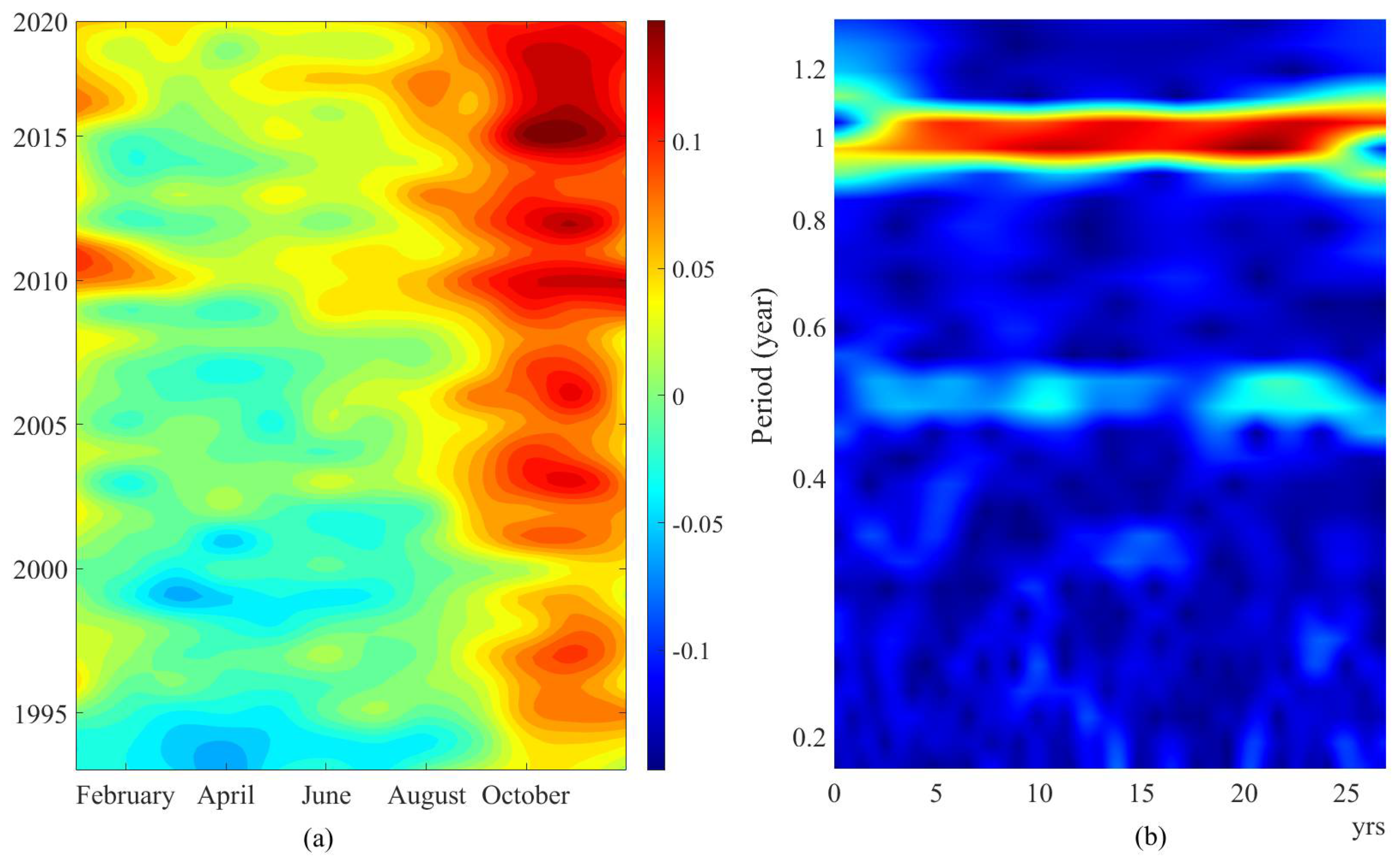
We also observed a clear time lag between both MSLA time series in the upwelling and open ocean areas during the annual cycle, with the former area being delayed with respect to the latter (Figure 3). Positive anomalies were centred in October in the oceanic zone (Figure 2a), while in the upwelling region, the highest values appeared in November (Figure 4a). This fact explained the time lag observed in Figure 3. Moreover, positive sea level anomalies were sharper in the upwelling zone, reaching values up to 15 cm in recent years. The intensification of positive anomalies increased since the 2010s, as well as the monthly range of occurrence. This phenomenon also occurs in the open ocean, but with lower MSLA values. Similarly, monthly negative anomalies range of incidence also decreased over the years for both zones. The sea level in the upwelling zone, by contrast, showed a bi-annual cycle (Figure 4b). The horizontal red band indicates a persistent annual periodicity throughout the years of this study. However, a diffuse and intermittent 6-month frequency was also observed (light-blue in Figure 4b).
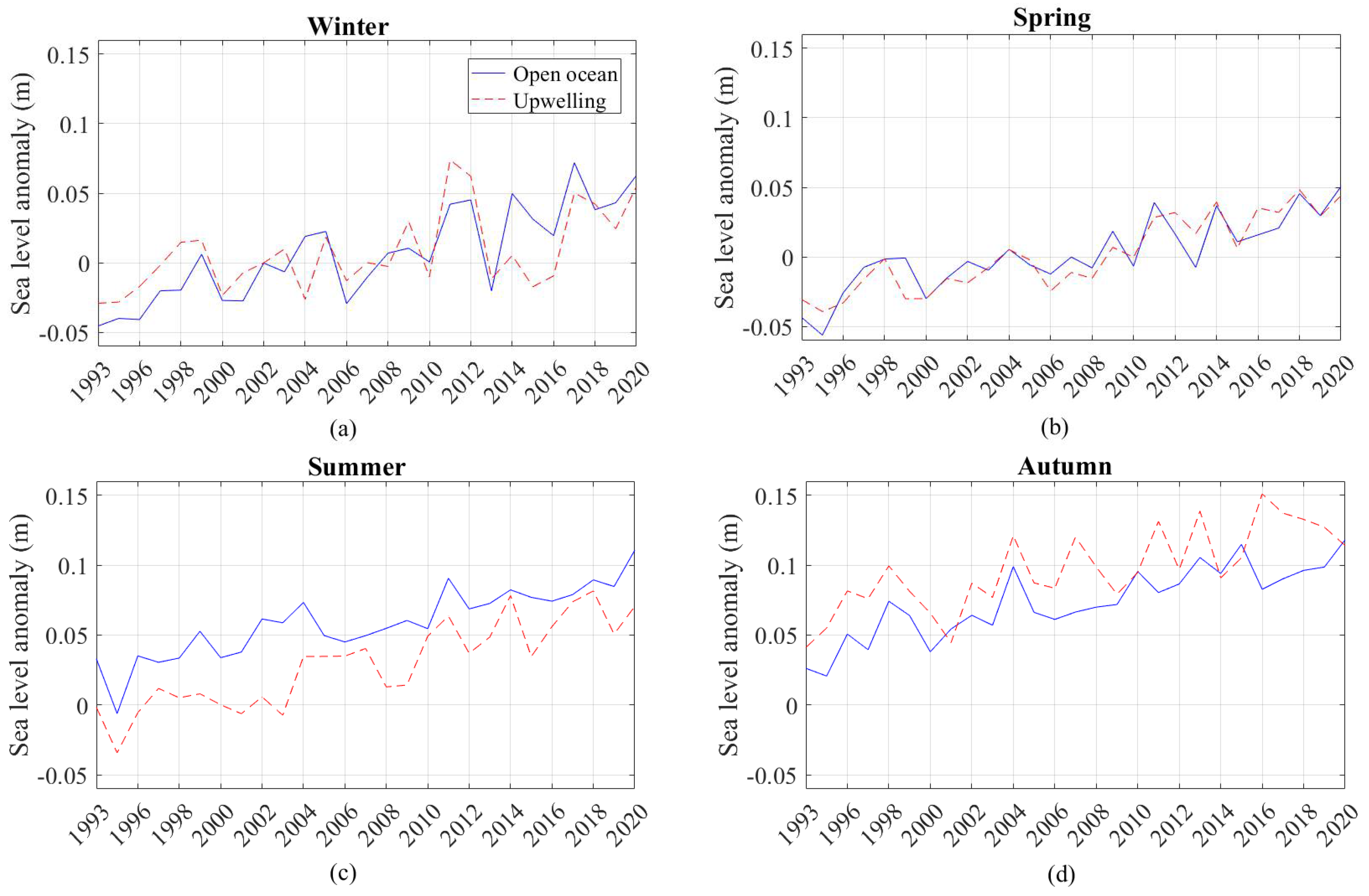
To study the seasonality in both the upwelling and oceanic areas, we selected the central months for each season (February for winter, May for spring, August for summer, and November for autumn). The most intense anomalies were found during autumn (Figure 5d), being more pronounced in the upwelling region (red dashed line). Similar trends were observed in both areas during winter and spring (Figure 5a,b). However, anomalies during summer were higher in the oceanic zone with respect to the upwelling zone (Figure 5c). This was due to the temperature difference between the open ocean and the upwelling zone during the Trade Wind season, promoting Ekman transport in the coastal area.
Slope values (Table 2) were positive during all seasons. Steep slopes were found during winter in the oceanic zone and during summer in the upwelling area, reaching values around 0.34 cm·y−1 in both zones, which implies a total sea level variation of 9.18 cm for the entire period of study in such seasons. In the oceanic zone, the lowest anomalies of −4.53 and −5.61 cm occurred during winter and spring, respectively, owing to colder SST during this period. Conversely, the maximum values were found during autumn in both the oceanic and upwelling areas, as expected (Figure 2a, Figure 4a and Figure 5b and Table 2).
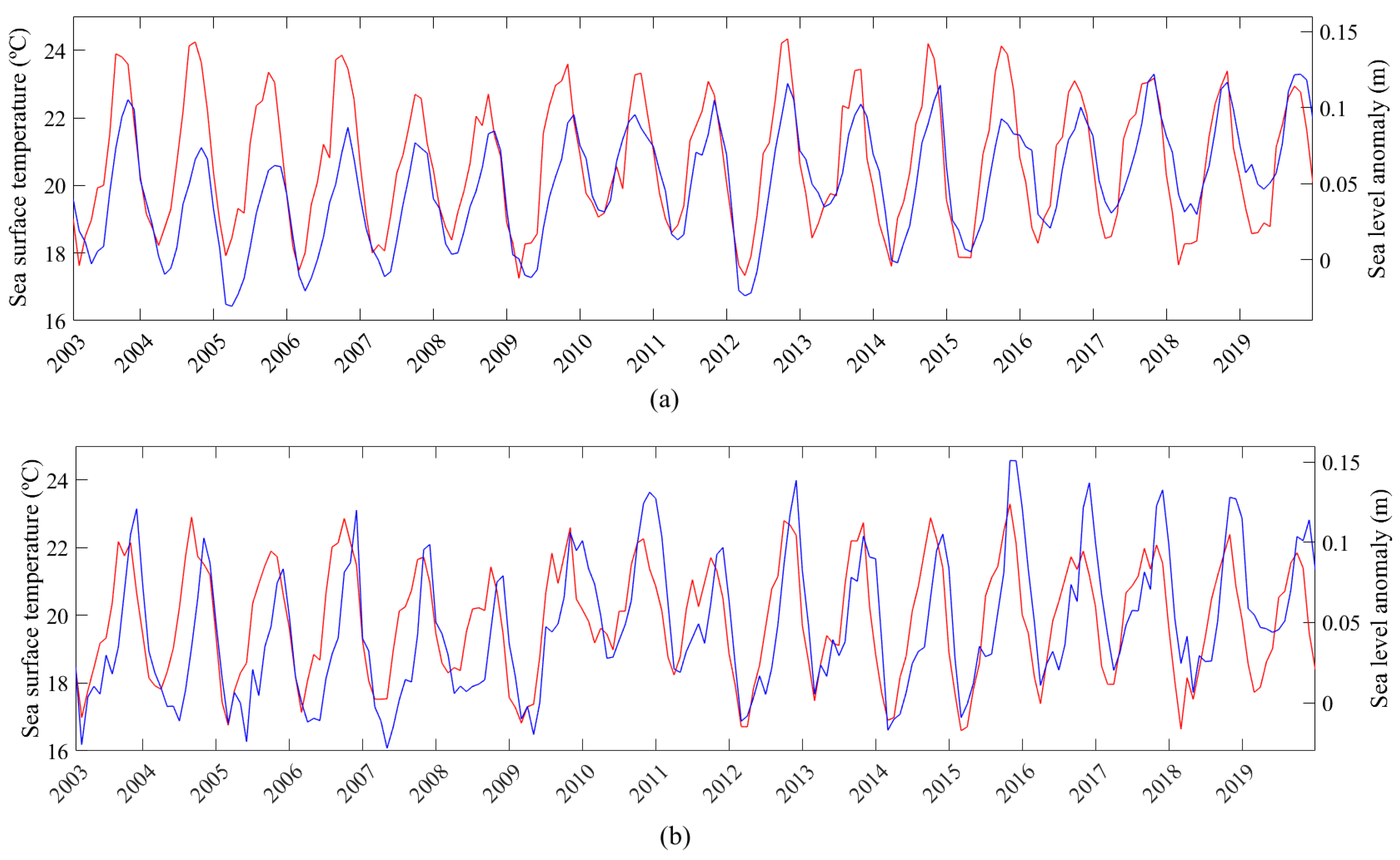
We compared our sea level data with climate indices such as the North Atlantic Oscillation (NAO), the Atlantic Multidecadal Oscillation (AMO) (Enfield et al., 2001), Sea Surface Temperature (SST), and Chlorophyll-a (Chl-a) as an index of productivity (Table 3). We did not find significant correlations between the different variables (NAO, AMO, and Chl-a) and sea level data for the oceanic and upwelling areas. As expected, SST and MSLA were closely related (Figure 6) as changes in sea level are primarily driven by changes in the ocean heat content (thermal expansion). We found a significant correlation between both parameters in oceanic and upwelling areas (r = 0.7525, p < 0.001, r = 0.6522, p < 0.001, respectively). We found the highest correlation between sea level anomalies and SST with a time lag of 2 months in both areas (r = 0.8350, p < 0.001, r = 0.7752, p < 0.001, respectively).
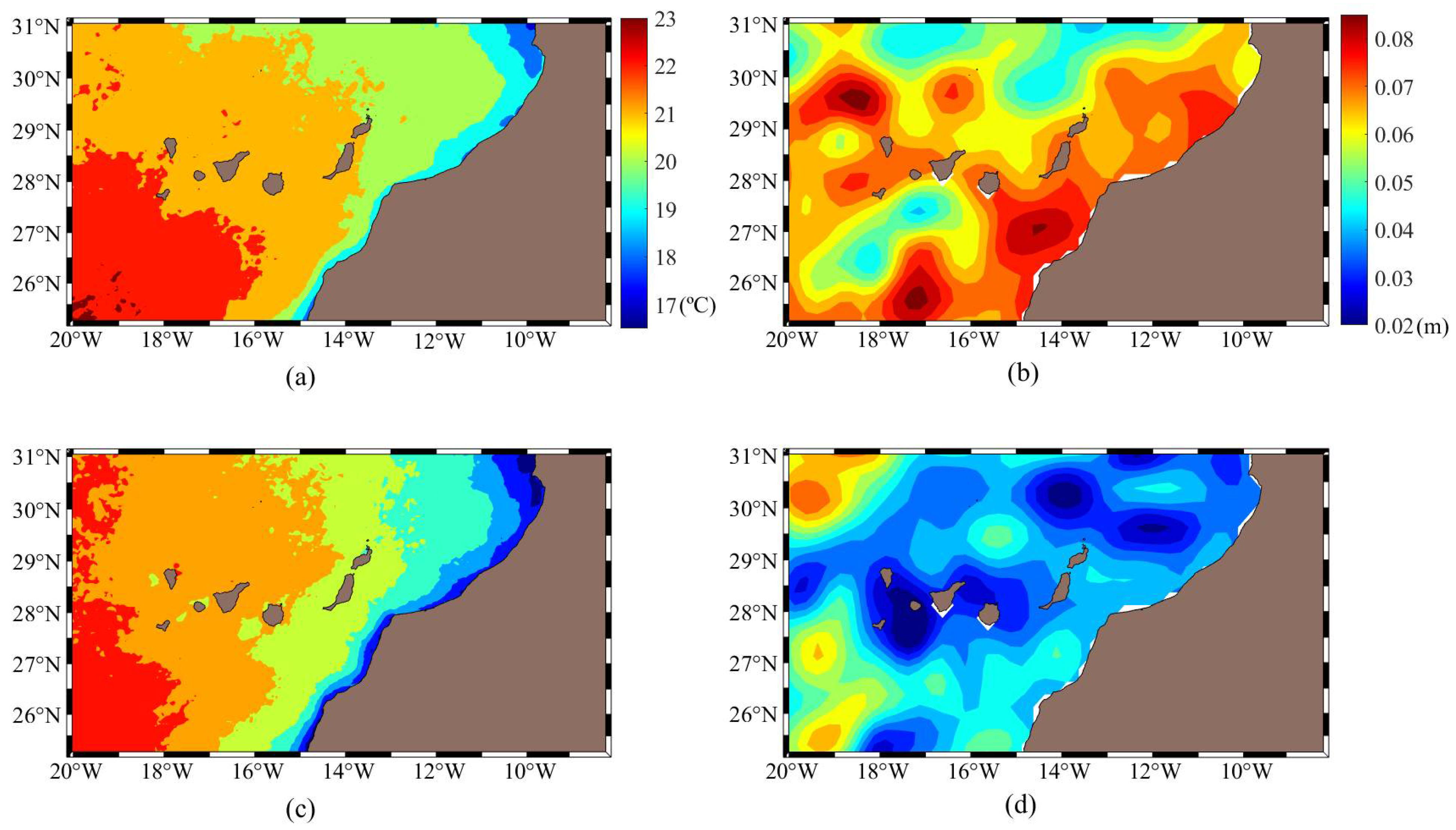
We selected a warm (2010) and a cold year (2012) to analyse the differences. During 2010, warm waters covered the entire Canary archipelago (compare Figure 7a,c), causing positive sea level anomalies around the archipelago (Figure 7b) due to thermal expansion. However, during 2012, the sea temperature around the archipelago was colder, causing negative sea level anomalies for the entire study area (Figure 7d).
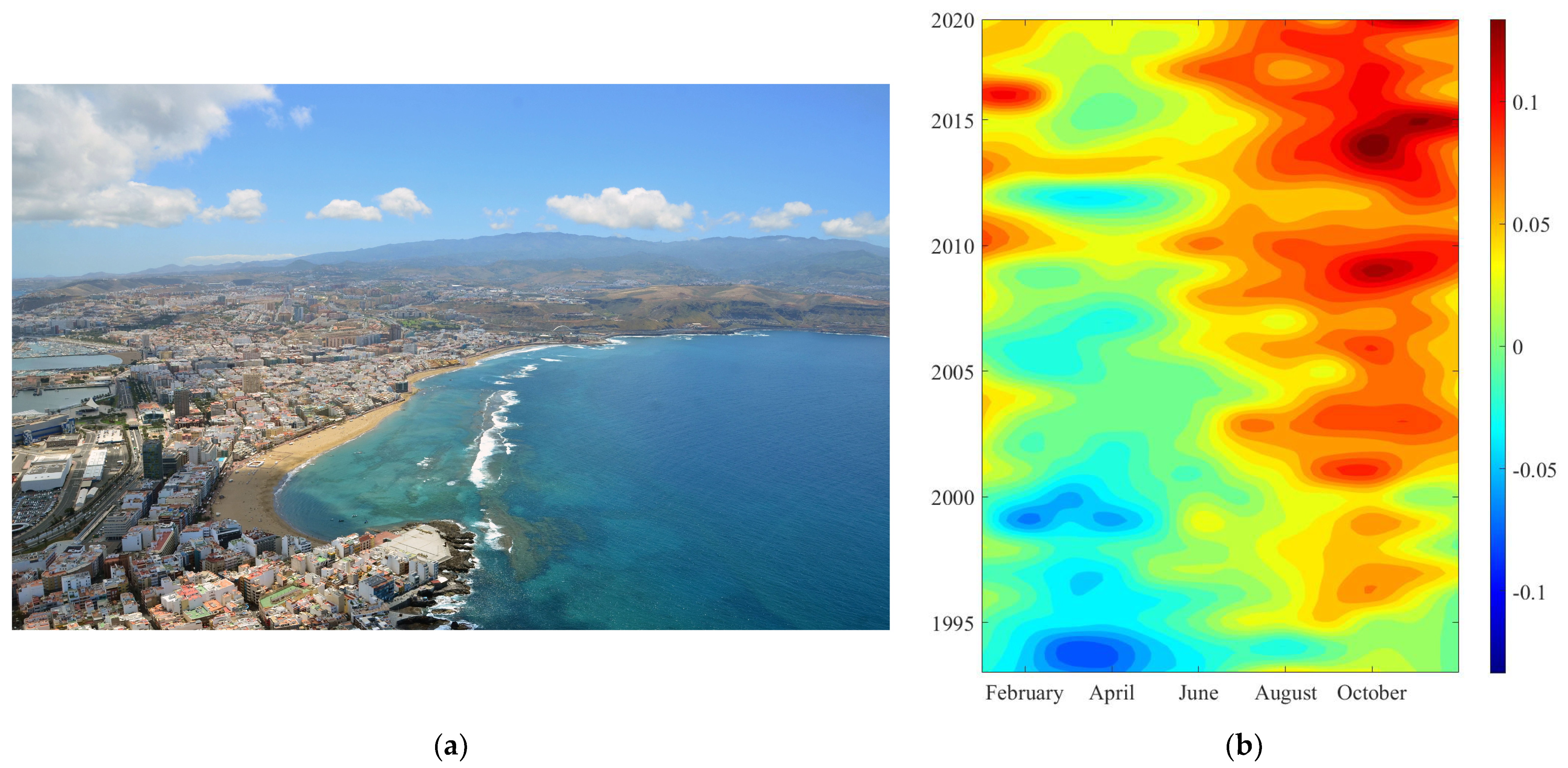
Additionally, we conducted a study on MSLA trends in the greatest urban beach of the Canarian archipelago, Las Canteras beach (28.1250° N, 15.3750° W), located in Las Palmas de Gran Canaria (Figure 1b, green dot). This is the largest and most densely populated municipality in the Canary Archipelago (about 400,000 inhabitants), and its beach represents a high socioeconomic value for the town [26]. In this zone, MSLA showed a similar pattern to the centre and south zone of the archipelago, and the slope of 0.026 cm/year implies a total rise of 8.42 cm over these 27 years of study. The average MSLA value was 3.49 cm and the most remarkable anomaly occurred during October 2014, reaching 14.43 cm. The main positive anomalies were found during autumn (red colour, Figure 8), specifically in October. These positive anomalies extend to June during the last years, increasing in magnitude and duration. Conversely, the negative anomalies disappear throughout the years of study. Considering the slope of the time series, the sea level prediction analysis for Las Canteras beach from 1993 to 2019 shows a sea level rise of about 18.10 and 33.40 cm for 2050 and 2100, respectively.
4. Discussion
In this study, we thoroughly analysed the monthly sea level change of the Canary Current and the eastern boundary upwelling system for the period from 1993 to 2019 using the MSLA product with the aim to visualize trends and changes in sea level. Over the last 27 years, MSLA experienced an increase in both study areas, implying a total average rise of 7.94 cm. There are no significant differences in the total average MSLA results between the two zones. To the best of our knowledge, this is the first time a detailed sea level analysis with satellite data has been performed in the Canary Current and the coastal upwelling area off Northwest Africa. Oceanic islands will suffer adverse consequences due to global warming and, in the Canary Islands, these alterations will entail risks derived from a foreseeable increase in the danger to certain meteorological phenomena [28]. Moreover, there are near coastal locations in Western Sahara some dozen meters below the sea level (e.g., Sebkha Tah). Thus, these areas will be highly impacted by future sea level increases as flooding of large areas of this territory will affect the population there.
However, regarding the annual cycle, there were changes between open ocean and the coastal upwelling region. The analyses carried out in open waters showed a marked annual pattern, reaching maximum values of MSLA in autumn, specifically during October. Thus, the ocean warms during summer and sea level reaches a maximum thermal expansion two months later, as observed from the lag between SST and MSLA in the time series analysis. However, the upwelling area showed a bi-annual pattern owing to the higher Ekman transport and the corresponding upwelling during summer. Our results clearly reflect the summer occurrence of the upwelling, as evidenced by lower sea level anomalies due to cooler waters during this period when compared with open ocean values. On the other hand, the most pronounced slopes were obtained during winter in the oceanic zone owing to warmer temperatures during this season after the mid-1990s (Figure 6). In addition, we obtained the most pronounced slope in the upwelling zone during summer, suggesting a decrease in the strength of the upwelling, as suggested in earlier studies [29,30,31,32]. In the Canary system, the negative trend in upwelling is closely connected to the low-frequency variability of the Atlantic Multidecadal Oscillation [33,34,35].
Regarding the local study in Las Canteras beach (Gran Canaria Island), the sea level continued to rise during this 27-year period (8.42 cm) and, if the same trend continues, it will reach 18.10 cm by 2050. Considering this, some areas of the beach will disappear during high tide, causing changes in coastal dynamics. Note that the economic growth of the Canary Islands, in general, and Gran Canaria in particular, is due to the development of the tourism industry. Since the arrival of mass tourism in the 1960s, beaches have been the showcase attraction. In this time span, the wide-ranging changes in the coastal occupation model have had a strong impact on the economy, society, culture, and the environment [36], with the landscape being a graphic representation of these changes [37]. For this reason, we consider this analysis to be of real importance because this is an area with significant environmental, social, and economic fragility. In addition, the local pattern is important for predicting the magnitude of regional variations of future changes.
Previous studies have addressed the sea level rise over different time spans, geographical zones, and using different datasets. Specifically, according to Gouzenes et al. [38], the global sea level rise was 3.3 mm year−1, with an acceleration of 0.1 mm y−2 over 1993–2019 data. On the other hand, the South Atlantic reached a mean value of 2.91 mm year−1 [39] during the same period, and more specifically, in the Subtropical Atlantic, a value of 2.6 mm year−1 was obtained by Dangendorf et al. [4] over the 1993–2015 period. These results demonstrate that sea level is not a homogeneous variable, as observed in previous studies, carried out with both remote sensing data and with in situ data [40,41,42]. Moreover, a non-uniform increase in sea level was identified since 1993 [43] for different sub-regions. For instance, an increase of 2.05 mm year−1 was observed for the Bay of Biscay region, while it was 3.98 mm year−1 for the Baltic Sea. On the other hand, the Black Sea level has increased at the rate of 3.2 mm/year since 1993 [44], and in the particular case of Emilia-Romagna Coast (Italy), a value of 2.8 mm/year was obtained by Meli et al. [45]. For this reason, sea level rise must be studied at the regional level. Recent studies in the Canary Islands area basically use in situ measurements. For example, Marcos et al. [46] observed a sea level rise at Tenerife of 2.096 mm/year from 1927 to 2012 using tide gauges. The work of Valdes et al. [47] addressed the sea level variability for the Canary Current Large Marine Ecosystem region using existing data from both tide gauges and a satellite altimeter. However, the remote sensing analysis only covered three locations, used a shorter time period (1993 to 2013), and used altimeter data with 1/3° spatial resolution. In any case, the results followed a similar trend with a mean increase of around 3.7 mm/year.
Our results indicate that the period of incidence of positive sea level anomalies has increased since 2010, covering almost every month of the year, mainly in the open ocean zone. This result is worrying because of the long-term consequences for the Canary Islands and the Western Sahara region, in particular coastal areas at high risk of flooding. Moreover, during the last 3 years, the behaviour of the MSLA has been relatively similar in the Canary archipelago and in the upwelling system. This phenomenon needs to be studied and further research and monitoring should be performed.
Our study may help to identify specific research requirements for different islands, which is important considering the complex and variable risks from climatic alterations, and the lack of necessary data for adequate planning. Additionally, our research could notably support further studies, as well as future actions aimed at the coastal risk mitigation and sustainable development of the Canary Islands, especially Gran Canaria Island coast. In addition, the seasonal study and the novel analysis comparing open water and upwelling zones could encourage other scientists to monitor differences between both types of waters.
5. Conclusions
A thorough analysis of sea level variability over the last 27 years was performed around the Canary archipelago. Two different areas, the open ocean around the Canary Islands and the coastal upwelling zone off Northwest Africa, were considered, as well the annual and seasonal trends. The sea level has not stopped rising in both study areas, implying a total variation of ≈8 cm since 1993. Our results corroborate that sea level has a marked annual pattern in open ocean, linked mainly to changes in SST. By contrast, the upwelling zone showed a bi-annual cycle owing to the maximum intensity of Trade Winds, and thus Ekman transport, during summer. The SST and MSLA are closely related in both study zones (r = 0.753 and r = 0.652 for open ocean and upwelling, respectively). However, they reach the maximum level of correlation with a two-month lag. The most intense anomalies occur in autumn in both zones, indicating that the ocean warms up during the summer and, two months later, the sea level reaches its maximum thermal expansion. These results corroborate future consequences produced by climate change. We predict a sea level rise of 18.10 cm by 2050 in the city area of Las Palmas de Gran Canaria. Finally, we show the need to increase sea level characterisation at the basin and sub-basin scales, improving knowledge on regional climate change effects and the associated risks in coastal areas. Future research will focus on comparing altimeter data with in situ measurements in a specific location to analyse the correlation between both data sources. We also plan to process high-resolution optical and lidar imagery to perform a detailed study of the future effects of sea level rise in critical areas.
Author Contributions
Conceptualization, J.M., D.R.-E. and S.H.-L.; methodology, J.M., D.R.-E. and S.H.-L.; formal analysis, N.M.-B.; investigation, N.M.-B.; data curation, N.M.-B.; writing—original draft preparation, N.M.-B.; writing—review and editing, J.M., D.R.-E. and S.H.-L.; supervision, J.M., D.R.-E. and S.H.-L. All authors have read and agreed to the published version of the manuscript.
Funding
This study was funded by project DESAFÍO (PID2020-118118RB-I00) from the Spanish Ministry of Science and Innovation, projects SUMMER (Grant Agreement 817806) and TRIATLAS (Grant Agreement 817578) from the European Union (EU) Horizon 2020 Research and Innovation Programme, and the EU Interreg projects of cooperation RESCOAST (MAC2/3.5b/314) and MACCLIMA (MAC2/3.5b/254) from the V-A MAC 2014–2020.
Institutional Review Board Statement
Not applicable.
Informed Consent Statement
Not applicable.
Data Availability Statement
The monthly sea level anomalies data were collected and made freely available by Aviso (Archiving, Validation, and Interpretation of Satellite Oceanographic data), which is a service set up by CNES to process, archive, and distribute data and products from altimetry satellite missions (https://www.aviso.altimetry.fr/en/home.html, last access: 4 March 2022). SST and CHL data are collected, processed, calibrated, validated, archived, and distributed by the NASA Ocean Biology Processing Group (OBPG) of the NASA Ocean Data Processing System (ODPS) (https://oceancolor.gsfc.nasa.gov/, last access: 4 March 2022). The AMO index data were obtained at NOAA/ESRL/PSD1 and are available at https://www.esrl.noaa.gov/psd/data/timeseries/AMO/ (last access: 4 March 2022). The NAO index data were obtained at NOAA (https://www.ncdc.noaa.gov/teleconnections/nao/ (last access: 4 March 2021)).
Acknowledgments
We acknowledge CNES (Centre National D’Études Spatiales) and NASA (National Aeronautics and Space Administration) for making their data available in this study.
Conflicts of Interest
The authors declare no conflict of interest.
References
- Oppenheimer, M.; Glavovic, B.C.; Hinkel, J.; van de Wal, R.; Magnan, A.K.; Abd-Elgawad, A.; Cai, R.; Cifuentes-Jara, M.; DeConto, R.M.; Ghosh, T.; et al. Sea Level Rise and Implications for Low-Lying Islands, Coasts and Communities. In IPCC Special Report on the Ocean and Cryosphere in a Changing Climate; Pörtner, H.-O., Roberts, D.C., Masson-Delmotte, V., Zhai, P., Tignor, M., Poloczanska, E., Mintenbeck, K., Alegría, A., Nicolai, M., Okem, A., et al., Eds.; Cambridge University Press: Cambridge, UK; New York, NY, USA, 2019; pp. 321–445. [Google Scholar] [CrossRef]
- Cazenave, A.; Nerem, R.S. Present-day Sea level change: Observations and causes. Rev. Geophys. 2004, 42, 1077–1083. [Google Scholar] [CrossRef]
- Nerem, R.S.; Beckley, B.D.; Fasullo, J.T.; Hamlington, B.D.; Masters, D.; Mitchum, G.T. Climate-change–driven accelerated sea-level rise detected in the altimeter era. Proc. Natl. Acad. Sci. USA 2018, 115, 2022–2025. [Google Scholar] [CrossRef] [PubMed] [Green Version]
- Dangendorf, S.; Hay, C.; Calafat, F.M.; Marcos, M.; Piecuch, C.G.; Berk, K.; Jensen, J. Persistent acceleration in global sea-level rise since the 1960s. Nat. Clim. Chang. 2019, 9, 705–710. [Google Scholar] [CrossRef] [Green Version]
- Horton, B.P.; Rahmstorf, S.; Engelhart, S.E.; Kemp, A.C. Expert assessment of sea-level rise by AD 2100 and AD 2300. Quat. Sci. Rev. 2014, 84, 1–6. [Google Scholar] [CrossRef]
- Vermeer, M.; Rahmstorf, S. Global Sea level linked to global temperature. Proc. Natl. Acad. Sci. USA 2009, 106, 21527–21532. [Google Scholar] [CrossRef] [Green Version]
- Jevrejeva, S.; Grinsted, A.; Moore, J.C. Upper limit for sea level projections by 2100. Environ. Res. Lett. 2014, 9, 104008. [Google Scholar] [CrossRef] [Green Version]
- Overpeck, J.T.; Otto-Bliesner, B.L.; Miller, G.H.; Muhs, D.R.; Alley, R.B.; Kiehl, J.T. Paleoclimatic evidence for future ice-sheet instability and rapid sea-level rise. Science 2006, 311, 1747–1750. [Google Scholar] [CrossRef] [Green Version]
- McMillan, M.; Shepherd, A.; Sundal, A.; Briggs, K.; Muir, A.; Ridout, A.; Wingham, D. Increased ice losses from Antarctica detected by CryoSat-2. Geophys. Res. Lett. 2014, 41, 3899–3905. [Google Scholar] [CrossRef]
- Rignot, E.; Mouginot, J.; Morlighem, M.; Seroussi, H.; Scheuchl, B. Widespread, rapid grounding line retreat of Pine Island, Thwaites, Smith, and Kohler glaciers, West Antarctica, from 1992 to 2011. Geophys. Res. Lett. 2014, 41, 3502–3509. [Google Scholar] [CrossRef] [Green Version]
- Morlighem, M.; Rignot, E.; Mouginot, J.; Seroussi, H.; Larour, E. Deeply incised submarine glacial valleys beneath the Greenland ice sheet. Nat. Geosci. 2014, 7, 418–422. [Google Scholar] [CrossRef]
- Cazenave, A.; Dominh, K.; Guinehut, S.; Berthier, E.; Llovel, W.; Ramillien, G.; Larnicol, G. Sea level budget over 2003–2008: A reevaluation from GRACE space gravimetry, satellite altimetry and Argo. Global Planet. Chang. 2009, 65, 83–88. [Google Scholar] [CrossRef] [Green Version]
- Levitus, S.; Antonov, J.I.; Boyer, T.P.; Locarnini, R.A.; Garcia, H.E.; Mishonov, A.V. Global ocean heat content 1955–2008 in light of recently revealed instrumentation problems. Geophys. Res. Lett. 2009, 36, L07608. [Google Scholar] [CrossRef]
- Cazenave, A.; Llovel, W. Contemporary sea level rise. Annu. Rev. Mar. Sci. 2010, 2, 145–173. [Google Scholar] [CrossRef] [Green Version]
- Willis, J.K.; Chambers, D.P.; Kuo, C.Y.; Shum, C.K. Global sea level rise: Recent progress and challenges for the decade to come. Oceanography 2010, 23, 26–35. [Google Scholar] [CrossRef]
- Leuliette, E.W.; Willis, J.K. Balancing the sea level budget. Oceanography 2011, 24, 122–129. Available online: http://www.jstor.org/stable/24861273 (accessed on 7 July 2022). [CrossRef]
- Barton, E.D.; Arıstegui, J.; Tett, P.; Cantón, M.; Garcıa-Braun, J.; Hernández-León, S.; Wild, K. The transition zone of the Canary Current upwelling region. Prog. Oceanogr. 1998, 41, 455–504. [Google Scholar] [CrossRef]
- Hernández-León, S.; Gomez, M.; Arístegui, J. Mesozooplankton in the Canary Current System: The coastal–ocean transition zone. Prog. Oceanogr. 2007, 74, 397–421. [Google Scholar] [CrossRef]
- Rodríguez, J.M.; Hernández-León, S.; Barton, E.D. Mesoscale distribution of fish larvae in relation to an upwelling filament off Northwest Africa. Deep Sea Res. Part I 1999, 46, 1969–1984. [Google Scholar] [CrossRef]
- Martín, J.L.; Marrero, M.V.; Del Arco, M.; Garzón, V. Aspectos clave para un plan de adaptación de la biodiversidad terrestre de Canarias al cambio climático. In Los Bosques y la Biodiversidad Frente al Cambio Climático: Impactos, Vulnerabilidad y Adaptación en España; Ministerio de Agricultura, Alimentación y Medio Ambiente: Madrid, Spain, 2015; Chapter 53; pp. 573–580. [Google Scholar]
- Nurse, L.A.; Mclean, R.F.; Agard, J.; Briguglio, L.P.; Duvat-Magnan, V. Small islands. In Climate Change 2014: Impacts, Adaptation, and Vulnerability. Part B: Regional Aspects. Contribution of Working Group II to the Fifth Assessment Report of the Intergovernmental Panel on Climate Change; Barros, V.R., Field, C.B., Dokken, D.J., Mastrandrea, M.D., Mach, K.J., Bilir, T.E., Chatterjee, M., Ebi, K.L., Estrada, Y.O., Genova, R.C., et al., Eds.; Cambridge University Press: Cambridge, UK, 2014; pp. 1613–1654. [Google Scholar]
- Kelman, I.; Khan, S. Progressive climate change and disasters: Island perspectives. Nat. Hazards 2013, 69, 1131–1136. [Google Scholar] [CrossRef]
- Ablain, M.; Philipps, S.; Picot, N.; Bronner, E. Jason-2 global statistical assessment and cross-calibration with Jason-1. Mar. Geod. 2010, 33, 162–185. [Google Scholar] [CrossRef]
- Ablain, M.; Legeais, J.F.; Prandi, P.; Marcos, M.; Fenoglio-Marc, L.; Dieng, H.B.; Cazenave, A. Satellite altimetry-based sea level at global and regional scales. Surv. Geophys. 2017, 38, 7–31. [Google Scholar] [CrossRef]
- Neuer, S.; Cianca, A.; Helmke, P.; Freudenthal, T.; Davenport, R.; Meggers, H.; Llinás, O. Biogeochemistry and hydrography in the eastern subtropical North Atlantic gyre. Results from the European time-series station ESTOC. Prog. Oceanogr. 2007, 72, 1–29. [Google Scholar] [CrossRef]
- Di Paola, G.; Aucelli, P.P.C.; Benassai, G.; Iglesias, J.; Rodríguez, G.; Rosskopf, C.M. The assessment of the coastal vulnerability and exposure degree of Gran Canaria Island (Spain) with a focus on the coastal risk of Las Canteras Beach in Las Palmas de Gran Canaria. J. Coast Conserv. 2018, 22, 1001–1015. [Google Scholar] [CrossRef]
- Fotos Aaéreas de Canarias. Available online: https://www.fotosaereasdecanarias.com/ (accessed on 7 July 2022).
- Olcina, J. Turismo y cambio climático: Una actividad vulnerable que debe adaptarse. Investig. Turísticas 2012, 4, 1–32. [Google Scholar] [CrossRef] [Green Version]
- Vallis, G.K. El Niño: A chaotic dynamical system? Science 1986, 232, 243–245. [Google Scholar] [CrossRef] [PubMed]
- Saji, N.H.; Goswami, B.N.; Vinayachandran, P.N.; Yamagata, T. A dipole mode in the tropical Indian Ocean. Nature 1999, 401, 360–363. [Google Scholar] [CrossRef] [PubMed]
- Gómez-Gesteira, M.; De Castro, M.; Álvarez, I.; Lorenzo, M.N.; Gesteira, J.L.G.; Crespo, A.J.C. Spatio-temporal upwelling trends along the canary upwelling system (1967–2006). Ann. N. Y. Acad. Sci. 2008, 1146, 320–337. [Google Scholar] [CrossRef]
- Barton, A.D.; Pershing, A.J.; Litchman, E.; Record, N.R.; Edwards, K.F.; Finkel, Z.V.; Ward, B.A. The biogeography of marine plankton traits. Ecol. Lett. 2013, 16, 522–534. [Google Scholar] [CrossRef]
- Narayan, N.; Paul, A.; Mulitza, S.; Schulz, M. Trends in coastal upwelling intensity during the late 20th century. Ocean Sci. 2010, 6, 815–823. [Google Scholar] [CrossRef] [Green Version]
- Pardo, P.C.; Padn, X.A.; Gilcoto, M.; Farina-Busto, L.; Pérez, F.F. Evolution of upwelling systems coupled to the long-term variability in sea surface temperature and ekman transport. Clim. Res. 2011, 48, 231–246. [Google Scholar] [CrossRef] [Green Version]
- Cropper, T.E.; Hanna, E.; Bigg, G.R. Spatial and temporal seasonal trends in coastal upwelling off northwest africa, 1981–2012. Deep Sea Res. Part I 2014, 86, 94–111. [Google Scholar] [CrossRef] [Green Version]
- Garín-Muñoz, T.; Montero-Martín, L.F. Tourism in the Balearic Islands: A dynamic model for international demand using panel data. Tour. Manag. 2007, 28, 1224–1235. [Google Scholar] [CrossRef]
- Peña-Alonso, C.; Pérez-Chacón, E.; Hernández-Calvento, L.; Ariza, E. Assessment of scenic, natural and cultural heritage for sustainable management of tourist beaches. A case study of Gran Canaria island (Spain). Land Use Policy 2018, 72, 35–45. [Google Scholar] [CrossRef]
- Gouzenes, Y.; Léger, F.; Cazenave, A.; Birol, F.; Bonnefond, P.; Passaro, M.; Benveniste, J. Coastal sea level rise at Senetosa (Corsica) during the Jason altimetry missions. Ocean Sci. 2020, 16, 1165–1182. [Google Scholar] [CrossRef]
- Ruiz-Etcheverry, L.A.; Saraceno, M. Sea level trend and fronts in the South Atlantic Ocean. Geosciences 2020, 10, 218. [Google Scholar] [CrossRef]
- Stammer, D.; Cazenave, A.; Ponte, R.M.; Tamisiea, M.E. Causes for contemporary regional sea level changes. Annu. Rev. Mar. Sci. 2013, 5, 21–46. [Google Scholar] [CrossRef] [Green Version]
- Cazenave, A.; Meyssignac, B.; Ablain, M.; Balmaseda, M.; Bamber, J.; Barletta, V.; Wouters, B. Global sea-level budget 1993-present. Earth Syst. Sci. Data 2018, 10, 1551–1590. [Google Scholar] [CrossRef] [Green Version]
- Legeais, J.-F.; Ablain, M.; Zawadzki, L.; Zuo, H.; Johannessen, J.A.; Scharffenberg, M.G.; Fenoglio-Marc, L.; Fernandes, M.J.; Andersen, O.B.; Rudenko, S.; et al. An improved and homogeneous altimeter sea level record from the ESA Climate Change Initiative. Earth Syst. Sci. Data 2018, 10, 281–301. [Google Scholar] [CrossRef] [Green Version]
- Iglesias, I.; Lorenzo, M.N.; Lázaro, C.; Fernandes, M.J.; Bastos, L. Sea level anomaly in the North Atlantic and seas around Europe: Long-term variability and response to North Atlantic teleconnection patterns. Sci. Total Environ. 2017, 609, 861–874. [Google Scholar] [CrossRef]
- Kostianaia, E.A.; Kostianoy, A.G. Regional Climate Change Impact on Coastal Tourism: A Case Study for the Black Sea Coast of Russia. Hydrology 2021, 8, 133. [Google Scholar] [CrossRef]
- Meli, M.; Olivieri, M.; Romagnoli, C. Sea-Level Change along the Emilia-Romagna Coast from Tide Gauge and Satellite Altimetry. Remote Sens. 2021, 13, 97. [Google Scholar] [CrossRef]
- Marcos, M.; Puyol, B.; Calafat, F.M.; Woppelmann, G. Sea level changes at Tenerife Island (NE Tropical Atlantic) since 1927. J. Geophys. Res. Oceans 2013, 118, 4899–4910. [Google Scholar] [CrossRef] [Green Version]
- Valdés, L.; Déniz-González, I. Oceanographic and Biological Features in the Canary Current Large Marine Ecosystem; IOC-UNESCO: Paris, France, 2015; Available online: http://hdl.handle.net/1834/9135 (accessed on 7 July 2022).
Figure 1.
(a) Geographical area of Atlantic Macaronesia during boreal summer season. Inset shows the study zone. The sea level anomaly (m) is coloured. (b) Sampling data around the Canary Islands are represented as blue dots for those used for the open ocean study of sea level, while the red dots are representative of the upwelling zone. The black dot was chosen as it coincides with the long-term temperature monitoring at the ESTOC time-series station. The green dot represents a coastal beach (Las Canteras) located in the most populated city of the archipelago (Las Palmas de Gran Canaria).

Figure 2.
MSLA in the oceanic waters of the Canary Current. (a) Monthly variation in MSLA (m) over the years. (b) Wavelet analysis of the sea level anomaly.
Figure 2.
MSLA in the oceanic waters of the Canary Current. (a) Monthly variation in MSLA (m) over the years. (b) Wavelet analysis of the sea level anomaly.

Figure 3.
Comparative analysis of time series of upwelling (red dashed line) and open ocean (blue line) sea level anomalies.
Figure 3.
Comparative analysis of time series of upwelling (red dashed line) and open ocean (blue line) sea level anomalies.

Figure 4.
MSLA in the upwelling zone. (a) Monthly variation in MSLA (m) over the years. (b) Wavelet analysis of the sea level anomaly.
Figure 4.
MSLA in the upwelling zone. (a) Monthly variation in MSLA (m) over the years. (b) Wavelet analysis of the sea level anomaly.

Figure 5.
Time series of the sea level anomaly during the central months of each season in the oceanic zone (blue line) and the upwelling area (red dashed line). (a) Winter (February), (b) spring (May), (c) summer (August), and (d) autumn (November).
Figure 5.
Time series of the sea level anomaly during the central months of each season in the oceanic zone (blue line) and the upwelling area (red dashed line). (a) Winter (February), (b) spring (May), (c) summer (August), and (d) autumn (November).

Figure 6.
SST (left axis, red line) and MSLA (right axis, blue line) time series from 2003 to 2019. (a) Oceanic zone. (b) Upwelling zone.
Figure 6.
SST (left axis, red line) and MSLA (right axis, blue line) time series from 2003 to 2019. (a) Oceanic zone. (b) Upwelling zone.

Figure 7.
(a) Mean SST (°C) averaged for 2010. (b) Mean MSLA (m) averaged for 2010. (c) Mean SST (°C) averaged for 2012. (d) Mean MSLA (m) averaged for 2012.
Figure 7.
(a) Mean SST (°C) averaged for 2010. (b) Mean MSLA (m) averaged for 2010. (c) Mean SST (°C) averaged for 2012. (d) Mean MSLA (m) averaged for 2012.

Figure 8.
(a) Las Canteras beach. Adapted photo with permission from [27]. (b) Monthly variations in MSLA (m) in Las Canteras beach from 1993 to 2019.
Figure 8.
(a) Las Canteras beach. Adapted photo with permission from [27]. (b) Monthly variations in MSLA (m) in Las Canteras beach from 1993 to 2019.


Table 1.
Statistical analysis of sea level anomaly (cm) over 1993–2019, both inclusive. Values are the result of averaging all subareas and each one independently. The average column is the mean of the 14 sampling points we used for the study.
Table 1.
Statistical analysis of sea level anomaly (cm) over 1993–2019, both inclusive. Values are the result of averaging all subareas and each one independently. The average column is the mean of the 14 sampling points we used for the study.
| Average | North | Centre | South | Upwelling | |
|---|---|---|---|---|---|
| Average | 3.483 | 3.509 | 3.586 | 3.468 | 3.351 |
| Max | 12.226 | 13.942 | 13.303 | 14.883 | 15.096 |
| Min | −6.327 | −7.604 | −6.417 | −7.197 | −6.120 |
| Slope | 0.024 | 0.024 | 0.026 | 0.025 | 0.023 |
| Offset | −0.502 | 0.387 | −0.637 | −0.598 | 0.462 |
Table 2.
Statistical analysis of sea level anomaly (cm) for open ocean and the upwelling area over the period from January 1993 to December 2019.
Table 2.
Statistical analysis of sea level anomaly (cm) for open ocean and the upwelling area over the period from January 1993 to December 2019.
| Open Ocean | Upwelling | |||||||
|---|---|---|---|---|---|---|---|---|
| Winter | Spring | Summer | Autumn | Winter | Spring | Summer | Autumn | |
| Mean | 0.678 | 0.212 | 5.881 | 7.357 | 0.763 | 0.183 | 2.934 | 9.697 |
| Max | 7.195 | 5.054 | 11.071 | 11.816 | 7.390 | 4.837 | 8.157 | 15.090 |
| Min | −4.534 | −5.614 | −0.610 | 2.073 | −2.900 | −3.923 | −3.417 | 4.113 |
| Slope | 0.348 | 0.279 | 0.270 | 0.277 | 0.197 | 0.297 | 0.336 | 0.279 |
| Offset | −4.196 | −3.539 | 2.096 | 3.481 | −1.999 | −3.980 | −1.764 | 5.794 |
Table 3.
Correlation analysis of sea level anomaly with weather phenomena and different oceanic parameters for open ocean and upwelling areas. North Atlantic Oscillation (NAO), Atlantic Multidecadal Oscillation (AMO), Chlorophyl-a (CHL), and Sea Surface Temperature (SST). Correlation values (r) are statistically significant for all variables (p < 0.001).
| Open Ocean | Upwelling | ||||||
|---|---|---|---|---|---|---|---|
| NAO | AMO | CHL | SST | NAO | AMO | CHL | SST |
| −0.1341 | 0.3542 | −0.3566 | 0.7525 | −0.0952 | 0.3303 | −0.4687 | 0.6522 |
Publisher’s Note: MDPI stays neutral with regard to jurisdictional claims in published maps and institutional affiliations. |
© 2022 by the authors. Licensee MDPI, Basel, Switzerland. This article is an open access article distributed under the terms and conditions of the Creative Commons Attribution (CC BY) license (https://creativecommons.org/licenses/by/4.0/).
Share and Cite
MDPI and ACS Style
Marrero-Betancort, N.; Marcello, J.; Rodríguez-Esparragón, D.; Hernández-León, S. Sea Level Change in the Canary Current System during the Satellite Era. J. Mar. Sci. Eng. 2022, 10, 936. https://doi.org/10.3390/jmse10070936
AMA Style
Marrero-Betancort N, Marcello J, Rodríguez-Esparragón D, Hernández-León S. Sea Level Change in the Canary Current System during the Satellite Era. Journal of Marine Science and Engineering. 2022; 10(7):936. https://doi.org/10.3390/jmse10070936
Chicago/Turabian StyleMarrero-Betancort, Nerea, Javier Marcello, Dionisio Rodríguez-Esparragón, and Santiago Hernández-León. 2022. "Sea Level Change in the Canary Current System during the Satellite Era" Journal of Marine Science and Engineering 10, no. 7: 936. https://doi.org/10.3390/jmse10070936
Note that from the first issue of 2016, this journal uses article numbers instead of page numbers. See further details here.