A Measurement System to Monitor Propulsion Performance and Ice-Induced Shaftline Dynamic Response of Icebreakers

Abstract

Polar navigation entails challenges that affect the continuation of ship operations in severe ice conditions. Due to ice-propeller interaction, propulsion shafting segments are often at a high risk of failure. Efficient methods for shaft line design are hence needed to ensure the safety of ice-going vessels and propulsion reliability. To this end, full-scale measurements have proven essential to support the development of ship-design tools and updated safety regulations for ice-going vessels. This paper presents a unique integrated measurement system that employs measuring equipment to monitor Polar-Class vessel performance and shaft line dynamics during ice navigation. The system was installed on board the Canadian Coast Guard (CCG) icebreaker Henry Larsen. This experimental concept aims to monitor the shaft’s torque and thrust fluctuations during ice navigation to obtain information about the ship’s propulsion efficiency. In the paper, we describe the arrangement of the measurement system and the components it features. Finally, we present preliminary datasets acquired during two icebreaking expeditions. This work is framed into a broader research project, which includes the long-term objective to determine a correlation between sea ice conditions and the dynamic response of shaft lines.

1. Introduction

1.1. Environmental and Economic Framework

Over the last few decades, the economic and strategic interests involving the exploitation of the Arctic Ocean region have become a pivotal factor in numerous industrial sectors of the world economy. Global warming is the most significant phenomenon that makes anthropic activities possible in Polar waters, as the increasing ice melting process augments the viability of shipping routes [1,2,3,4]. Two primary industrial sectors are mainly involved: energy resource supply chain and freight transportation. In the first case, the vast availability of oil and liquid natural gas in the Arctic region represents an attractive stimulus for the energy sector to fulfill the global demand for energetic sources [5,6]. In the second case, the recent expansion of the global trade system led to a significant increase in Polar route utilization [2,7,8].

On the other hand, the utilization of shipping routes in the northernmost seas has been expanding, and it is expected to increase over the next few decades [1,9,10]. Consequently, the increment in all-year-round marine traffic through the Arctic Ocean entails several issues concerning pollution and in particular greenhouse gas emissions. Overall, the general outcome resulting from extensive Arctic shipping depicts a worsening effect on the environment due to shipping-related pollutants, as shown in [11,12,13,14]. Gong et al. provide a thorough analysis of the marine traffic effects on atmospheric pollution in the Canadian Arctic region, with a temporal span until 2030 [15].

The pollution generated by Arctic-going vessels significantly affects the economic sustainability of Polar shipping. Guaranteeing high proficiency levels for ships devised to operate in Polar environments is a challenging task, which requires accurate optimization plans to minimize the ship operations’ costs and concurrently ensure the employment of updated technology [14,16]. Therefore, updated regulation frameworks are necessary to make Arctic-going vessels comply with minimum requirements in terms of exhaust gas emissions, propulsion efficiency, and on-board safety [17,18]. A detailed treatise on marine systems reliability criteria and environmental protection measures can be found in [19].

1.2. Role of the Marine Industry

The design and construction of ice-going vessels have recently acquired high importance due to the increase in demand for new Polar-Class ships. Propulsion plants assume particular relevance in the design process of polar vessels: the structural properties of those systems and their components require particular consideration in order to be adequate for Arctic navigation [20,21,22,23]. In particular, ice collisions with propeller blades represent a crucial phenomenon that endangers the integrity of shafting systems and may compromise the manoeuvring capability of ships. Studying the operational conditions of ice-going vessels is key to assessing the probability of damage or failure of shaftlines [24].

Over the recent decades, the ice-propeller interaction process has been investigated through ice towing tank tests to determine its characteristics and how it relates to the hydrodynamic load [25,26,27,28]. In [27], the authors outlined an experimental methodology to identify the superimposed components of the combined ice and hydrodynamic load on propellers. A numerical model to estimate the ice loads on a podded propeller is presented in [29], where a model-scale pod is employed to validate the numerical results obtained through panel-method FEA. Model tests are often limited in providing results that can be reliably transferred to full-scale scenarios. Moreover, the utilization of model ice in towing tank experiments may lead to remarkable discrepancies with the actual ice effects.

Therefore, full-scale measurements are fundamental to sustain the advancement of ice-going vessels’ shipbuilding and ensuring that safety regulations remain up to date. Multi-objective, full-scale measurement campaigns aboard different types of Arctic vessels were carried out in the past to monitor the ship propulsion operation along with the ice-induced excitation on the hull and propellers. In particular, Williams et al. monitored the CCG icebreaker Henry Larsen during level ice navigation [30], and Suominen et al. studied the ice-induced loads on the hull of the Polar Supply Research Vessel Agulhas II [31,32]. Regarding merchant ships, in [33] the authors considered the case of an Arctic-Class bulk carrier; the full-scale, ice-induced impacts on the CP propeller of a ferry ship are studied through a measurement chain with cutting-edge instrumentation in [34].

Accurate measures of the dimensions of ice floes are essential to categorize the surrounding ice conditions and the resulting ice-induced excitation on ship structures. Sophisticated equipment such as stereoscopic cameras or laser detectors can be employed to get three-dimensional images of the sea ice [35,36,37]; in these cases, special post-processing software is necessary to elaborate the raw data. More specific ice block properties such as type, shape, age and concentration are measured and analyzed in [38]. Structural measurements and ice condition visual data need to be integrated to define the operating scenarios of ships. On this matter, a joint Finnish and South-African research team conducted an extensive measurement campaign project on board an icebreaker and a research vessel, which navigated across the area between Antarctica, South Africa, and Argentina [39,40]. The authors employed strain gauges to measure the torsional response of the shafts, whereas the sea ice conditions were empirically assessed from the command bridge. The authors carried out a statistical analysis of the shaft’s load distributions and fatigue [41]. The vibration data was then used to calculate the ice-propeller interaction torque [39,42,43].

1.3. Contribution of the Present Work

This paper outlines the features of a novel measurement system concept, which aims to monitor the propulsion performance and shaft line vibrations of Ice-Class vessels. The arrangement of the system was devised through a joint research project between Memorial University of Newfoundland (MUN, St. John’s, NL, Canada) and the National Research Council of Canada—Ocean, Coastal and River Engineering Research Centre (NRC-OCRE, St. John’s, NL, Canada). Specifically, the scope of this experimental design is to provide an integrated dataset that includes shafts’ dynamic response, sea ice conditions, and propulsion efficiency information during ice operations. In this work, we also present the application of the measurement system on board the CCG medium icebreaker Henry Larsen. The paper includes a series of example data acquired during two ice operation voyages of the vessel in two different Canadian Arctic regions. The work also provides a rare contribution to full-scale icebreaker performance data in Subarctic and high Arctic regions. The CCGS Henry Larsen has a unique multi-role service mission including open-water transits, nearshore icebreaking support, search and rescue, commercial escort, and northern resupply. The ship operates as far south as the St. Lawrence Seaway and in summer transits the northern latitudes of the Canadian Arctic Archipelago.

2. Materials and Methods

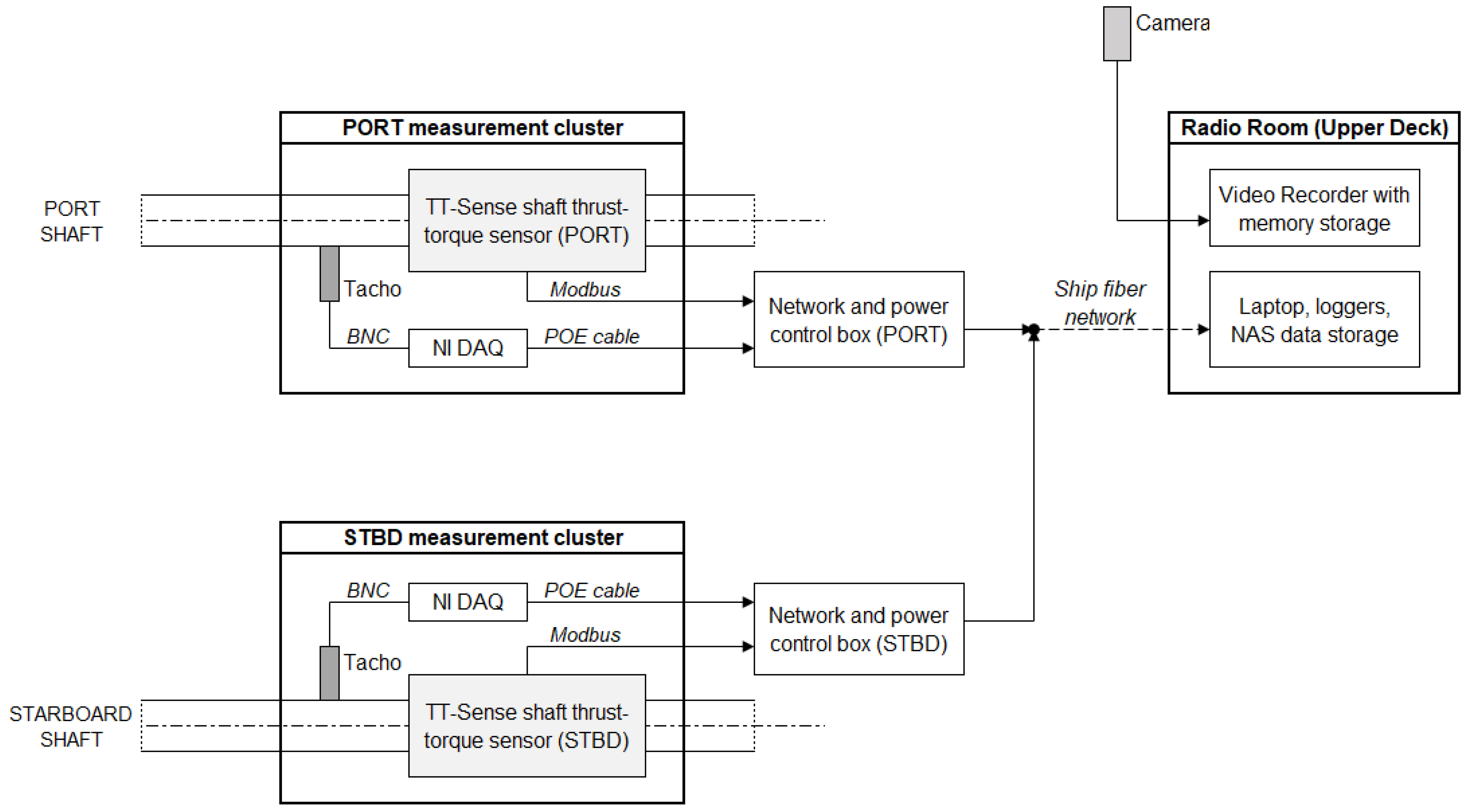
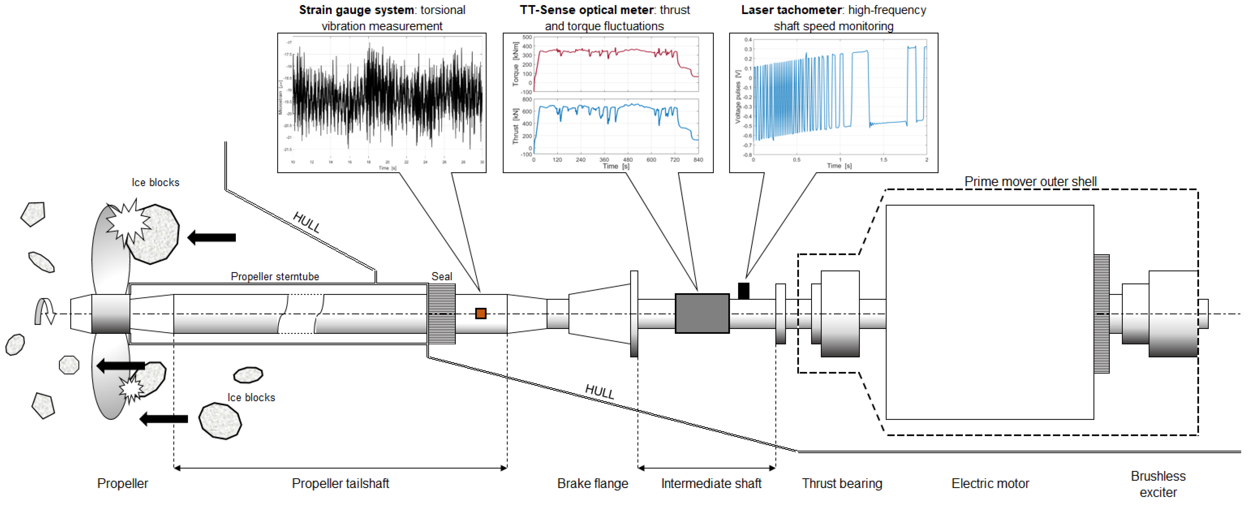
2.1. Overview of the Instrumentation Set and Description of the Case Study Vessel

In this section, we describe the components of the measurement system and their installation on board CCGS Henry Larsen. Optical meters are installed on both shafts to measure the thrust, torque, and speed fluctuations. Using laser torque meters to both measure ice-induced dynamic response and monitor ship propulsion performance is a novel element within the field of full-scale measurements in ice navigation. Besides, the transient-state rotational shaft speed drop is measured with laser tachometers to obtain high-frequency speed fluctuation signals, which are synchronized with the optical sensors. Concurrently, the sea ice conditions are monitored through a high-resolution digital camera mounted on the port-side, bridge-deck railing. Its operation principle is to record the ice blocks turning over against the hull; thus, the video frames are then processed to estimate the average sea ice thickness. In addition, the data acquisition system records the NMEA (Communication format defined by National Marine Electronics Association (NMEA) for marine utilization) data broadcast over the ship’s network; this dataset includes useful contextual information such as latitude and longitude, speed over ground and through water, weather conditions, and the status of the vessel’s air bubbler system.

Table 1. Outline of the measurement system components.

Device	Manufacturer	Description	Operation	Items	Location
TT-Sense${}^{\circledR }$ sensor	VAF Instruments	Optical LED rotating sensor	Low-frequency measurement of the shaft’s torque, thrust, speed fluctuations	2	Propeller shafting segments (Port, Starboard)
Laser tachometer	Brüel & Kjær	CCLD laser probe	High-frequency measurement of the shaft rotational speed	2	Propeller shafting segments (Port, Starboard)
Outdoor HD Camera	HIK Vision	Weatherproof IP-POE camera	Video recordings of the sea surface close to the hull	1	Side railing of a higher deck, pointing vertically downwards
MTi-300 (IMU sensor)	XSens	Attitude Heading and Reference System (AHRS)	20-Hz filtered 6-DOF acceleration, heading, pitch, roll motions	1	Communication Room (upper superstructure)

describes the instrumentation set for a twin-propeller vessel; details on their role and operation are included.

The main specifications of the CCG medium icebreaker Henry Larsen are reported in

Table 2. Main specifications of the icebreaker CCGS Henry Larsen.

Quantity		Value	Unit
Length overall	$L_{OA}$	99.8	[m]
Beam	B	19.6	[m]
Draught	d	7.3	[m]
Gross Tonnage	$GT$	6166	[GT]
Total propulsive power	$P_{TOT}$	12.2	[MW]
Propeller diameter	D	4.120	[m]
Maximum propeller’s rotational speed	$n_{max}$	180	[rpm]
Maximum transit speed	$V_S$	16	[kn]
Arctic Class certification	$AC$	4	[–]

. The ship was built in 1989 and has been operating across the Eastern Canadian Arctic region. The propulsion system of the vessel is a Diesel-Electric plant, in which three 4-stroke Diesel AC generators power the two electric motors of the twin shaft lines. The propellers are fixed-pitch type (FPP) with 4 blades ($Z=4$).

Figure 1 shows a schematic view of the arrangement, whereas Figure 2 illustrates the positions along the shaft line where the devices were installed. We used a torsional strain-gauge rosette to validate the shaft’s torque data measured by the optical sensors; the rosette’s location is indicated in Figure 2 as well.

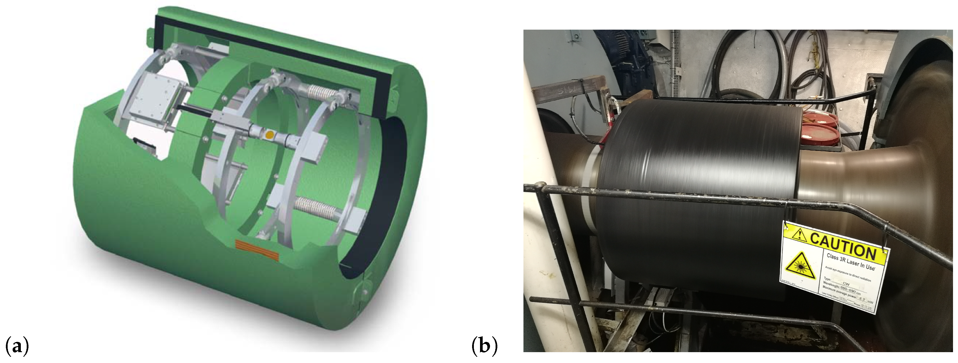
2.2. Shaft Thrust, Torque, Speed Measurements at Low Frequency

We installed one LED-optical sensor in each shaft line to measure the thrust and torque fluctuations as well as the instantaneous shaft speed with low-frequency output. In particular, we fixed the devices on the intermediate shaft segments, which are comprised between the brake wheel and the motor shaft flange; the shaft’s diameter is 477 mm. The principle of operation of the TT-Sense${}^{\circledR }$ sensor is based on detecting the relative axial, and angular motions between two rings fixed on the shaft. LED pointers are fixed on one ring, whereas optical detectors are mounted on the other ring and paired with the LED pointers. The axial and torsional vibrations of the two shaft sections where the rings are fastened produce deviations of the LED beam positioning in the optical detectors, which are then converted into voltage signals. The rotating rings and LED sensors are powered through inductive coils that draw energy from a non-rotating, external circuit. The data signal is continuously transmitted from the rotor detectors to the stator control box via a wireless communication channel at 2.4 GHz. The output data is then processed to determine the time series of shaft thrust, torque, and rotational speed, with a sampling frequency of 5 Hz. The shaft’s thrust, torque, and power output signals are acquired with errors of 1.0%, 0.25%, and 0.25% respectively (The sensor’s specifications are available in the manufacturer’s manual: www.vaf.nl/media/1434/tt-sense-optical-thrust-and-torque-measuring-systems-english-tib-664-gb-0215.pdf, accessed on 31 March 2022).

Figure 3 shows a cross-section of the sensor (A drawing of the sensor can be retrieved from the manufacturer’s manual: www.vaf.nl/media/1434/tt-sense-optical-thrust-and-torque-measuring-systems-english-tib-664-gb-0215.pdf, accessed on 31 March 2022), where the shaft’s rings are represented, along with a photograph of the Starboard side sensor on board the vessel.

The TT-Sense${}^{\circledR }$ system is employed to record both the steady-state propulsion parameters and their transient perturbations induced by the ice-propeller interaction processes during ice operations. The low-frequency output data do not allow to perform a vibration analysis of the shaft, but they provide information about the peak amplitude of the torque shaft response caused by the ice-propeller interaction.

Long-term, full-scale thrust and torque measurements constitute a means of evaluating the model test facilities at NRC, in a wide range of ice severity conditions, i.e., the full range of ice thicknesses and strengths from first-year through to multi-year ice layers, as well as: (i) to evaluate the impact of hull and propulsion maintenance programs on performance; (ii) to support the improvement of operational fuel use; (iii) to support future icebreaker design and concept evaluation programs. Besides, a key advantage of using this sensor type is its reliability for long-term, continuous data measurement and storage; this fact will contribute to obtaining large datasets to characterize the icebreaker’s shaft line operations in several ice scenarios.

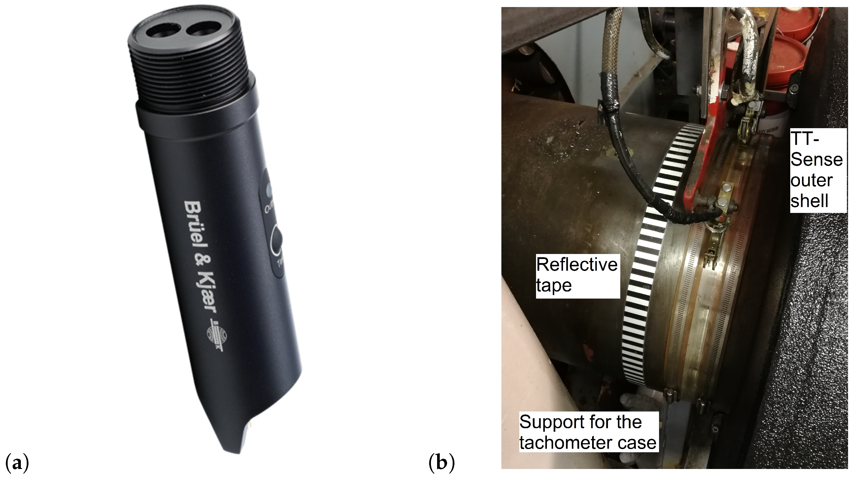
2.3. Shaft Speed Measurement at High Frequency

Each shaft is equipped with a laser tachometer for the high-frequency measurement of the rotational speed. For the equipment on board CCGS Henry Larsen, we employed the “Type 2981” tachometer model produced by Brüel & Kjær (Manufacturer’s specification sheet: www.bksv.com/media/doc/bp2448.pdf, accessed on 31 March 2022). Figure 4 shows the sensor and the installation setup. The tachometers are fixed on a vertical bracket, pointing toward a black-white striped reflective tape to produce a pulse signal (Figure 4b).

Overall, the reflective tape includes 100 white stripes and 100 black, all 7.5 mm wide, thereby providing 100 different pulses per shaft rotation. The pulse voltage has an error equal to 0.2 V with respect to the DC bias output level (Manufacturer’s specification sheet: www.bksv.com/media/doc/bp2448.pdf, accessed on 31 March 2022). Each tachometer is connected to a National Instruments (NI) data acquisition NI-9230 module and NI-cDAQ-9181 chassis through a BNC-type cable. The data is then transmitted to the Control Box through an Ethernet cable, as indicated in the diagram of Figure 1. The output signal has a frequency of 12.8 kHz, and we implemented the “Pulse Timing Method” to calculate the instantaneous shaft speed in rpm units [44]. Then, the resulting speed time history array is under-sampled at 100 Hz to reduce the necessary storage and the processing time to write the data in the memory disks. A Nyquist frequency of 50 Hz is adequate to include the main torsional vibration modes of the shaftline [45,46]. Therefore, from the time-domain rotational speed signals, we can determine the spectra of the angular velocity and the torsional displacement of both shafts.

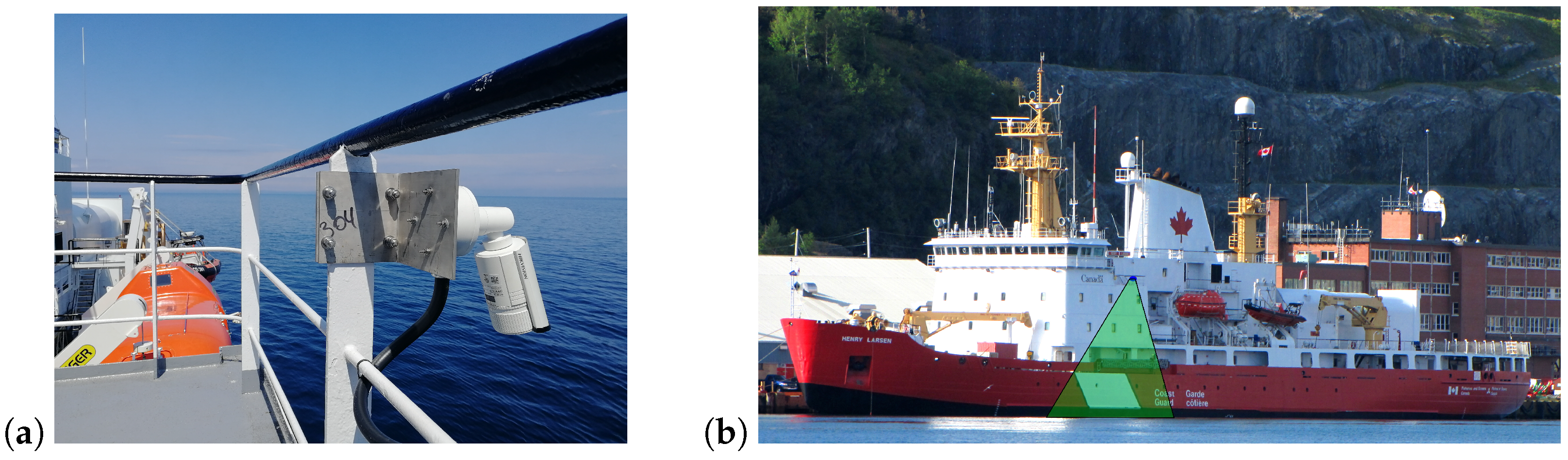
2.4. Ice Condition Monitoring

A high-definition, weatherproof IP camera is fixed to the Port-side railing of the Upper Deck, as shown in Figure 5 and positioned at a height of 13.6 m above sea level. The view is set to visualize the sea surroundings close to the ship hull by framing the water surface from a vertical line of view, as shown in Figure 5. The camera is manufactured by HIK Vision, and it has a maximum resolution of 2 MP. The screen resolution is 1920 × 1080 pixel, and the camera is equipped with a digital zoom feature. A Power over Ethernet (PoE) cabling route provides the electrical power to the camera and carries the data directly to the memory storage installed in the Network Video Recorder (NVR, Figure 1). The NVR encases a 6-TB hard drive, in which approximately three months of continuous recording files can be stored. For our purpose, we scheduled the video recording program to operate for 12 h a day.

The task of the camera is to monitor the sea ice conditions during icebreaking operations; the thickness property of ice layers is the target quantity to characterize different ice scenarios. To determine that, we consider the occurrences when the ice floes flip over due to the ship icebreaking advancement. In those cases, the thickness dimension of the ice blocks can be directly visualized from the camera’s point of view. In order to obtain the scale length ratio correlating actual sea-level distances to the video frame dimensions, we employed a floating square-shaped frame, in which ticks are marked 10 cm apart along its 60-cm-long sides. Figure 6 shows the frame as it appears in the recordings (Figure 6a) and a zoomed view of it, in which the minor marks are visible (Figure 6b). Once the scale ratio was set, we employed the software IC Measure${}^{\circledR }$ to process each video frame and determine the actual ice thickness values. Thereby, the ongoing ice conditions can be correlated to the shaft line dynamic response, which is monitored by the optical sensors.

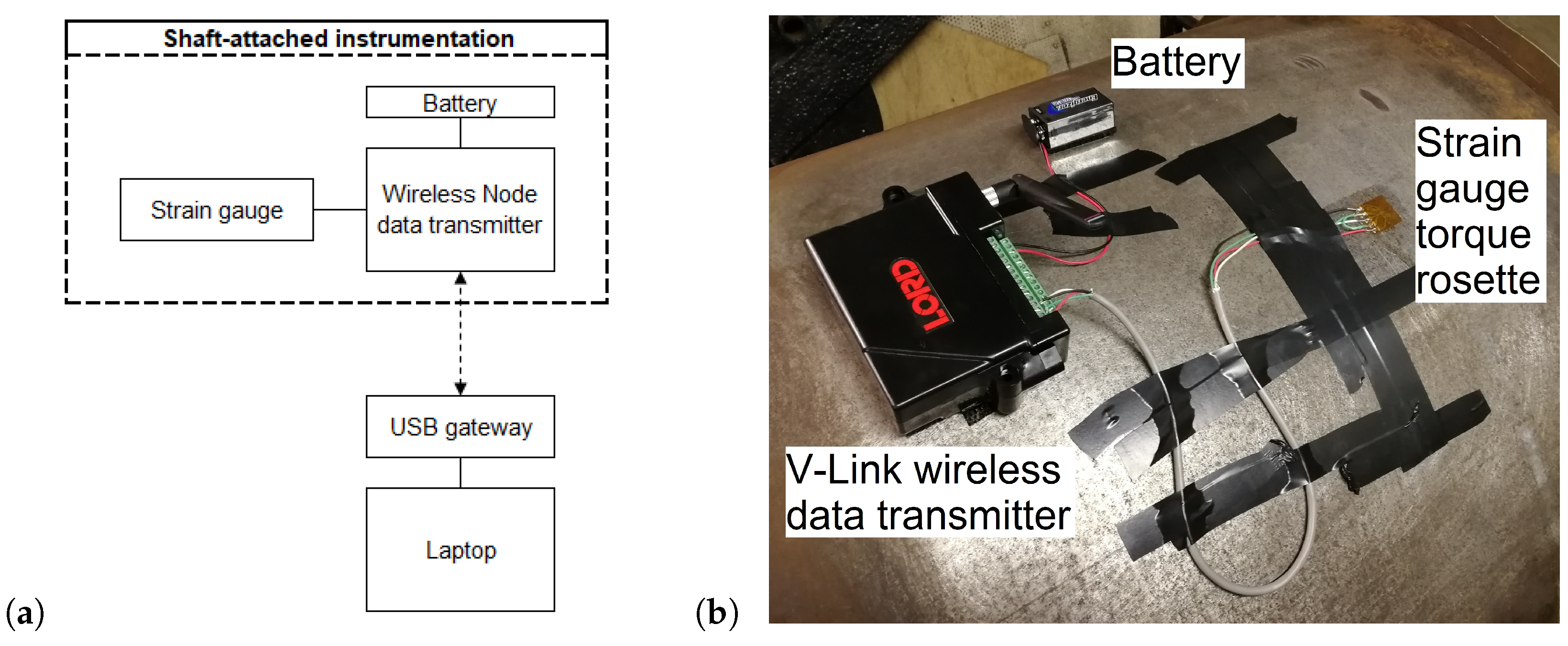
2.5. TT-Sense Torque Data Validation via Strain Gauge Measurements

To validate the shaft’s torque data measured by the TT-Sense, we installed a strain gauge system on the Starboard shaft to measure the dynamic torque at different propeller speeds during the vessel’s open-water trials on 10 August 2019. An analogous measurement arrangement was employed on board CCGS Terry Fox to monitor shafts’ vibrations at different loading conditions [47]. On CCGS Henry Larsen, the strain gauge outcomes were then compared with the concurrent measures of the TT-Sense. In the tests, the ship sailed around the northern end of the Avalon Peninsula in Newfoundland, Canada, with favourable weather, Sea State 2 conditions, and sea level deeper than 100 m.

The strain gauge we employed was a full-bridge Wheatstone rosette (model CEA-06-250US-350) manufactured by VPG Sensors. In detail, we attached the gauge to the second tailshaft segment of the shaft line, which has a diameter of $d_o=652$ mm and is located abaft the shaft line segment where the TT-Sense is installed (Figure 2). We positioned the grid pattern on the shaft surface according to [48]. The measurement output is the linear strain ($\epsilon$) along the 45-degree direction with respect to the shaft’s sectional plane. The strain gauge terminals were wired to a differential analog channel input on a V-Link-200 Node${}^{\circledR }$ wireless data transmitter provided by LORD Sensing Systems Corp. A WSDA-200-USB${}^{\circledR }$ gateway interfaced the node to a laptop. We employed the software “SensorConnect”${}^{\circledR }$ to set up the node and perform the measurement runs, which were carried out with a sampling frequency of 256 Hz. Figure 7 shows a schematic layout of the instrumentation (a) and its actual arrangement on board (b).

In the Wheatstone bridge strain gauge, the resistance of each coil is 350 $\Omega$, with a gauge factor equal to $k_g=2.10$ and a measurement error of 0.4%. The output analog voltage scale was calibrated through the shunt calibration circuit incorporated in the node. The maximum measurable linear strain is $\epsilon =5$%. The node transmission power to the USB gateway was set to 10 dBm (deciBel-mW). Overall, seven different steady-state speeds were considered during the sea trials, ranging from 66 rpm to 169 rpm. We acquired two 60-s long vibration data recordings in correspondence with each propeller loading condition. The average strain value ${\epsilon }_{\mathrm{mean}}$ for each speed n was calculated as the mean value of the corresponding signals. Finally, the steady-state shaft torque $Q_{\mathrm{shaft},\mathrm{Gauge}}\left(n\right)$ associated with a speed n is calculated as follows [48]:

$$Q_{\mathrm{shaft},\mathrm{Gauge}}\left(n\right)=\frac{\pi E\left(d_o^4-d_i^4\right)}{16d_o(1+\nu )}{\epsilon }_{\mathrm{mean}}\left(n\right)$$

(1)

where E and $\nu$ are the Young Modulus and Poisson Ratio of the shaft steel, respectively; $d_o$ and $d_i$ are the outer and inner diameter, respectively. In our case, $E=210$ GPa, $\nu =0.27$, $d_o=652$ mm, and $d_i=0$ mm. The $Q_{\mathrm{shaft},\mathrm{Gauge}}\left(n\right)$ obtained values are compared with the corresponding torque data measured by the Starboard TT-Sense ($Q_{\mathrm{shaft},\mathrm{TT},\mathrm{Stbd}}$). As an additional comparison term, we consider the shaft’s torque values observed from the ABB${}^{\circledR }$ monitoring panel in the Engine Control Room to check the coherence between the two measured data series. We used the $Q_{\mathrm{shaft},\mathrm{Gauge}}$ data as reference values because we could properly calibrate the strain gauge on the shaft, whereas the calibration details of the ABB monitor were unknown.

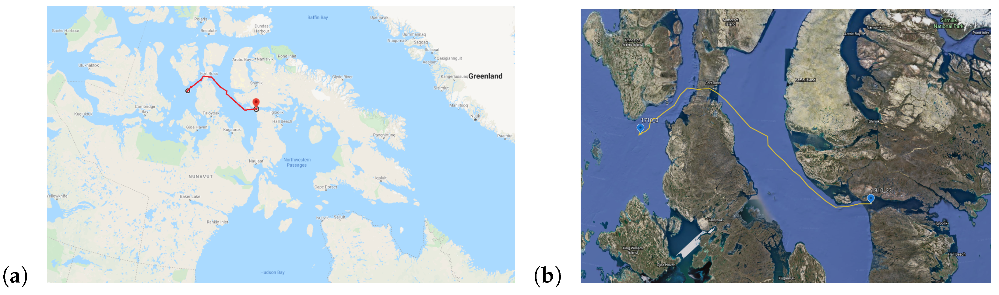
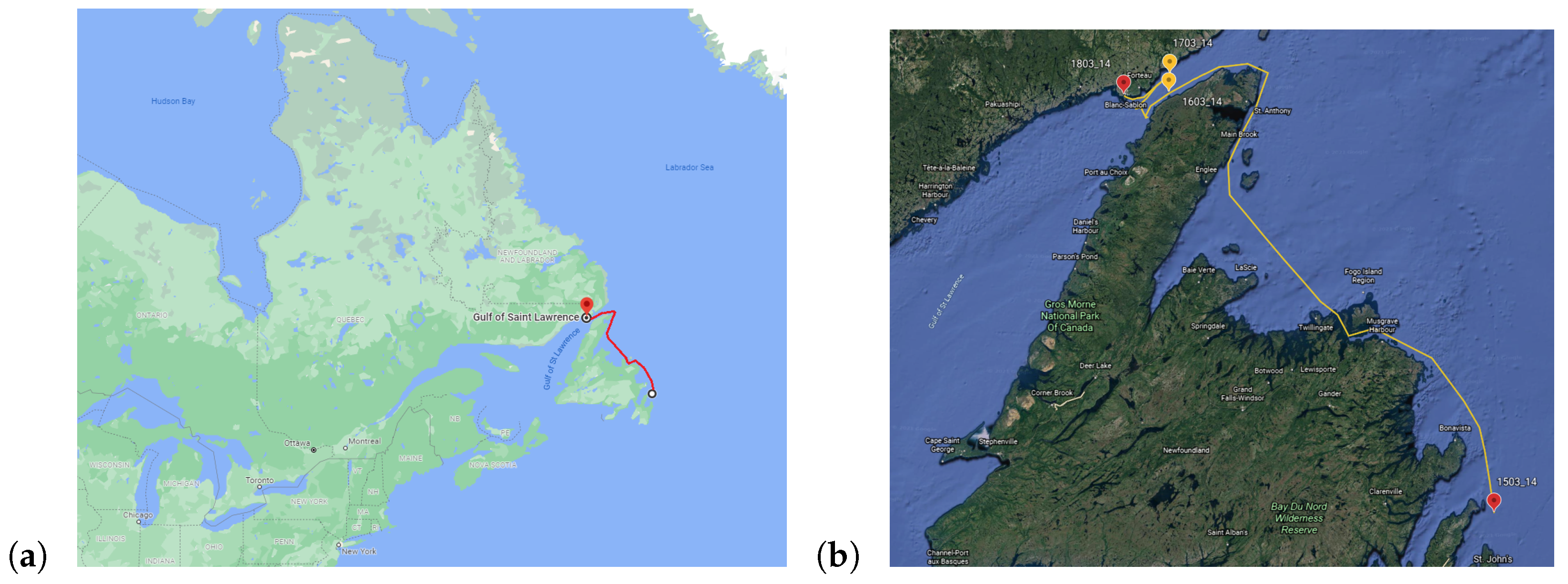
2.6. Trials in Ice-Covered Waters

In fall 2019, CCGS Henry Larsen performed icebreaking trials in the Nunavut Arctic region. On 17–18 October, the ship navigated from Franklin Strait to the Gulf of Boothia, passing through the Bellot Strait. Figure 8 shows CCGS Henry Larsen’s route on those two days. The route’s coordinates were obtained from the ship’s GPS logger, which tracks the vessel’s position with a frequency of 1 Hz. In the expedition, the ship encountered heavy ice conditions. During icebreaking operations, the TT-sense meters measured the ice-induced perturbations of shaft thrust, torque, and speed, whereas the outdoor camera filmed the ongoing sea ice conditions.

In winter 2020, the icebreaker carried out icebreaking operations in northern Newfoundland, Canada, across the strait region connecting Saint Barbe (NL) and Blanc Sablon (QC). The ship encountered ice also in the Twillingate and Fogo Island areas (central Newfoundland). The voyage took place on 15–18 March; its route is shown in Figure 9.

3. Results

3.1. Validation of the TT-Sense Torque Measures

Table 3. Torque values from the different sources, for seven speed levels.

Speed, n	${\mathit{Q}}_{\mathbf{shaft},\mathbf{Gauge}}$	${\mathit{Q}}_{\mathbf{shaft},\mathbf{TT},\mathbf{Stbd}}$	${\mathit{Q}}_{\mathbf{shaft},\mathbf{TT},\mathbf{Port}}$	${\mathit{Q}}_{\mathbf{shaft},\mathbf{Panel}}$	$\mathbf{\Delta }\mathit{Q}/{\mathit{Q}}_{\mathbf{shaft},\mathbf{Gauge}}$
[rpm]	[kNm]	[kNm]	[kNm]	[kNm]	[%]
66	37.3	23.8	27.5	43.4	36.2
84	55.7	41.0	37.8	56.8	26.4
106	83.5	66.4	63.2	81.1	20.5
126	114.2	100.8	96.2	113.7	11.7
148	151.4	132.2	127.0	142.0	12.7
159	174.2	152.8	164.6	156.2	12.3
169	201.1	179.3	182.8	192.1	10.8

reports the results of the torque values from the measurements performed with the strain gauge system ($Q_{\mathrm{shaft},\mathrm{Gauge}}$), the mean steady state torque data acquired by the TT-Sense sensors for both shafts ($Q_{\mathrm{shaft},\mathrm{TT},\mathrm{Stbd}}$ and $Q_{\mathrm{shaft},\mathrm{TT},\mathrm{Port}}$), along with the values read from the engine room control panel ($Q_{\mathrm{shaft},\mathrm{Panel}}$). In the last column the percentage discrepancy between $Q_{\mathrm{shaft},\mathrm{Gauge}}$ and $Q_{\mathrm{shaft},\mathrm{TT},\mathrm{Stbd}}$ ($\Delta Q/Q_{\mathrm{shaft},\mathrm{Gauge}}$) is shown.

The higher deviations in $\Delta Q/Q_{\mathrm{shaft},\mathrm{Gauge}}$ for the lower speed levels are due to the effects caused by: (i) the manoeuvring operations ongoing at those speeds; (ii) the superposition of bending and axial vibration modes of the shaft line; (iii) the different locations and shaft segment geometries where the TT-Sense sensors and strain gauge are positioned, as the selection of the sensors’ positions depended on the physical constraints in the engine room around the shaft lines. Figure 10 shows the vibration spectra acquired via the strain gauges at the lowest and highest shaft speeds (66 rpm and 169 rpm), where F and $BPF$ are the rotational frequency and the Blade Passing Frequency ($BPF=ZF$) respectively.

In Figure 10 we can observe that at very low frequencies the excitation at the 66 rpm speed is higher, also because $BP{F}_{66}$ falls below 5 Hz. This entails more significant fluctuations of the quasi-static torque in steady-state operations. Moreover, the spectra highlight how different modal shapes are excited at medium frequencies: at 26 Hz and 39 Hz the 66-rpm spectrum presents relevant peaks that are absent in the 169-rpm spectrum; vice versa at 37 Hz. The first torsional mode of the shaft line corresponds to 15 Hz [45].

Overall, Figure 11 shows the shaft torque outcomes from the strain gauge and the control panel as n varies, plus a regression curve for the $Q_{\mathrm{shaft},\mathrm{Gauge}}$ series.

Two distinct facts can be observed in Figure 11. Firstly, it shows the correspondence between the $Q_{\mathrm{shaft},\mathrm{Gauge}}$ values (black dots) and the $Q_{\mathrm{shaft},\mathrm{Panel}}$ ones (blue marks): this fact confirms the coherence between the two different measurement systems, for every shaft speed. Secondly, the $Q_{\mathrm{shaft},\mathrm{Gauge}}$ values demonstrate to fit a pure-quadratic curve as a function of n: this fact validates the propeller law assumption [49].

Specifically, in steady-state and open-water conditions the equivalence between $Q_{\mathrm{shaft},\mathrm{Gauge}}$ and the propeller-absorbed torque ($Q_{\mathrm{prop}}$) holds; the expression of $Q_{\mathrm{prop}}$ in this scenario can be expressed as follows [50]:

$$Q_{\mathrm{prop}}\left(n\right)=K_Q\left(n\right)\rho n^2{D}^5⟹Q_{\mathrm{prop}}\propto K_Q\left(n\right)n^2$$

(2)

where $K_Q$ is the propeller torque coefficient, $\rho$ is the water mass density, n is the propeller’s rotational speed in revolutions per second, D is the propeller diameter. The result of the regression analysis of $Q_{\mathrm{shaft},\mathrm{Gauge}}\left(n\right)$ (red curve in Figure 11) in terms of $R^2$ value shows that $Q_{\mathrm{shaft},\mathrm{Gauge}}\left(n\right)$ presents a pure-quadratic trend. Therefore, $K_Q\left(n\right)$ can be assumed as a constant parameter in Equation (2) in the case of FPP applications, and consequently $Q_{\mathrm{prop}}\left(n\right)$ can be considered to be a function of $n^2$ solely.

As an additional validation term of the TT-Sense output data, we compare the shaft’s effective power measured during short open-water time windows, at a constant speed, to model-scale results (ITTC 1957) that were measured in a 200-m towing tank in St. John’s (NL, Canada) [51]. The time history of the vessel’s longitudinal speed through water—obtained in a series of full-scale tests conducted on 30 October 2021—is shown in Figure 12; the analyzed data clips are indicated through shaded segments. In addition to the shown segments, we also use a longer data sequence measured on the following day, at a cruising speed of ≈17–18 kn. The model-scale experimental results [51] (black curve) are plotted along with the full-scale mean net power measured by the TT-Sense sensors (red dots) in Figure 13. The speed used for the comparison is the measured longitudinal speed in open-water conditions; however, no adjustments were made for wind, waves, or transverse water current. The full-scale results are proved to correspond to the model-scale estimated values.

3.2. Analysis of the Laser Tachometer Signal

During the vessel’s open-water sea trials, the shaft speed levels reported in Table 3 were reached progressively through successive steps. Figure 14 shows the Starboard shaft rotational speed across a time window 2000-s long. The plot shows the speed steps corresponding to 106, 126, 148, and 169 rpm, with fluctuations of n around the mean value in each level. Larger-amplitude oscillations occur at 148 rpm, which is reached after the transition from the 126 rpm step ($t\approx$ 900 s).

Figure 15 shows the spectrum of the angular speed signal ($\omega \left(f\right)$) at the 169 rpm speed level, which corresponds to the data of the last 400-s portion plotted in Figure 14, over the frequency range f up to the Nyquist frequency—50 Hz. The fundamental frequency, which corresponds to the shaft’s rotation rate (2.82 Hz), is clearly visible together with its harmonics up to the 10th order (28.2 Hz). Subsequently, the spectrum of the angular displacement ($\theta \left(f\right)$) can be derived numerically.

3.3. Ice-Induced Perturbations on the Shaft Dynamic Response

Figure 16 shows a 14-min excerpt of the Starboard TT-Sense data output, acquired during the October 2019 voyage. In the Bellot Strait icebreaking operations, the vessel encountered sea ice concentrations of 9/10ths and 10/10ths, with Stage-of-Development codes of 4, 5, 9, 8·, 9· indicating the presence of multi-year ice (Nomenclature of the Government of Canada’s Weather Services: www.canada.ca/en/environment-climate-change/services/ice-forecasts-observations/publications/interpreting-charts/chapter-1.html, accessed on 31 March 2022).

The physical quantities that constitute the output dataset from each sensor include the shaft’s torque Q (kNm), thrust T (kN), and speed n (rpm); in the plot, eight major perturbations are indicated and matched to the corresponding fluctuations of Q, T, and n.

In the 14-min time window, the vessel moves forward starting from zero speed; in the end, it stabilizes at 45 rpm. The vertical lines in Figure 16 match across time the onset of torque pulses with the corresponding fluctuations of thrust and shaft speed. In the plots, speed drop events that correspond to torque increases are more clearly visible in events 3 to 8; concerning the 1 and 2 marks, the torque pulses appear to lag behind the corresponding speed drop. The signals of Q and T are acquired with their respective signs, depending on the load direction, whereas n is recorded with positive signs disregarding the shaft’s rotation direction.

Figure 17 shows two frames of the video recordings during the time window considered above; the two frames (a) and (b) correspond to the instants around the events 2 and 6 shown in Figure 16. The procedure presented in Section 2.4 was used to calculate the thickness values of the ice floes.

Figure 18 shows the Inertial Measurement Unit (IMU) data acquired by the XSens device during the October 2019 voyage; the time window of the data clip corresponds to the one considered in Figure 16. Large vertical accelerations were experienced by the ship. The pitch angle changed dynamically during icebreaking operations, showing gradual bow’s angle rises up to ≈1.5 degrees before rapid drops. This behavior was likely due to the hull’s vertical motion during icebreaking processes. The roll angle fluctuations were limited to 2–3 degrees around the zero-degree position. All data series were acquired with the same sampling frequency of 20 Hz; the accuracy of the pitch and roll motions is 0.2 deg, whereas the accelerometer resolution is 15 $\mathsf{\mu }$g.

Besides, the data acquired by the torque sensor can be used to determine the fluctuations in shaft power (P), which is calculated as the absolute value of the product between shaft torque (Q) and rotational speed (n, in rpm) as follows:

$$P=\left|Q\right|\left(2\pi \frac{n}{60}\right)$$

(3)

The variability in shaft power during icebreaking operations is useful to indicate how the energy rate required by the electric motors fluctuates, and thus monitoring the status of the overall Diesel-electric power system through transient conditions. Figure 19 includes a 6-min dataset corresponding to forward-direction navigation in light ice, obtained during the March 2020 voyage. Specifically, the ice concentration encountered by the icebreaker ranged between 8/10ths and 10/10ths, with grey-ice type characterized by Stage-of-Development codes of 4, 5, 7 (Nomenclature of the Government of Canada’s Weather Services: www.canada.ca/en/environment-climate-change/services/ice-forecasts-observations/publications/interpreting-charts/chapter-1.html, accessed on 31 March 2022).

We calculated P through Equation (3) and the outcomes are plotted in parallel with the Q, T, n signals. From the shafts’ rotational speed curves, it can be noticed that the vessel was advancing at a semi-steady pace. Hence, the pattern of P is driven by the Q variability. Figure 20 shows the ice condition corresponding to this time interval.

In addition, the experimental data measured during icebreaking operations and manoeuvring is important to evaluate the effects of abrupt changes in shaft structural response and power output efficiency over short time intervals. Figure 21 shows an 8-min dataset obtained during backing and ramming manoeuvres in heavy ice conditions, and the corresponding sea scenario is depicted in Figure 22. In particular, the power value of 6 MW represents the upper limit that the three Diesel generators can deliver; it is reached at the two extremities of the time window and twice during the backing-ramming sequence. Additionally, the shaft speed is reported as a positive value disregarding the rotation direction. In the example of Figure 21, we can observe that the Starboard shaft reverses direction at about $t\approx$ 90 and 320 s. The curves indicate that the two shaft lines followed significantly different courses as the ship changed heading direction: while the Port-side shaft line maintained a more balanced power output, the Starboard-side propulsion line underwent three full excursions from zero to maximum power.

Figure 23 shows the data measured by the IMU XSens device in the time windows considered in the plots of Figure 19 and Figure 21. Significant oscillations in both pitch and roll angles occur, along with several vertical acceleration peaks. In particular, at the end of the time window in Figure 23b, the pattern of a ramming motion can be observed: large vertical acceleration matching a rise in pitch angle while the bow hits the ice layer.

4. Discussion

In this Section, the results shown in the previous parts are discussed sequentially.

• TT-Sense validation through strain gauges. As Figure 11 and Table 3 show, the $Q_{\mathrm{shaft},\mathrm{Gauge}}$ data correspond to the $Q_{\mathrm{shaft},\mathrm{Panel}}$ values, thus confirming the reliability of the strain gauge apparatus. The results in Table 3 indicate that the relative discrepancy ($\Delta Q/Q_{\mathrm{shaft},\mathrm{Gauge}}$) between the values measured by the TT-Sense and by the strain gauge decreases as the shaft’s speed increases. Since the TT-Sense and the strain gauge were installed on two different segments of the shaftline, the coupling of the axial, bending vibration modes at lower frequencies induces significant effects on the torsional responses in the two positions, as shown in Figure 10. In particular, the $Q_{\mathrm{shaft},\mathrm{TT},\mathrm{Stbd}}$ and $Q_{\mathrm{shaft},\mathrm{Gauge}}$ values differ significantly for $n<$ 100 rpm reflecting the higher uncertainty of the shaft’s torsional dynamics at lower speeds.
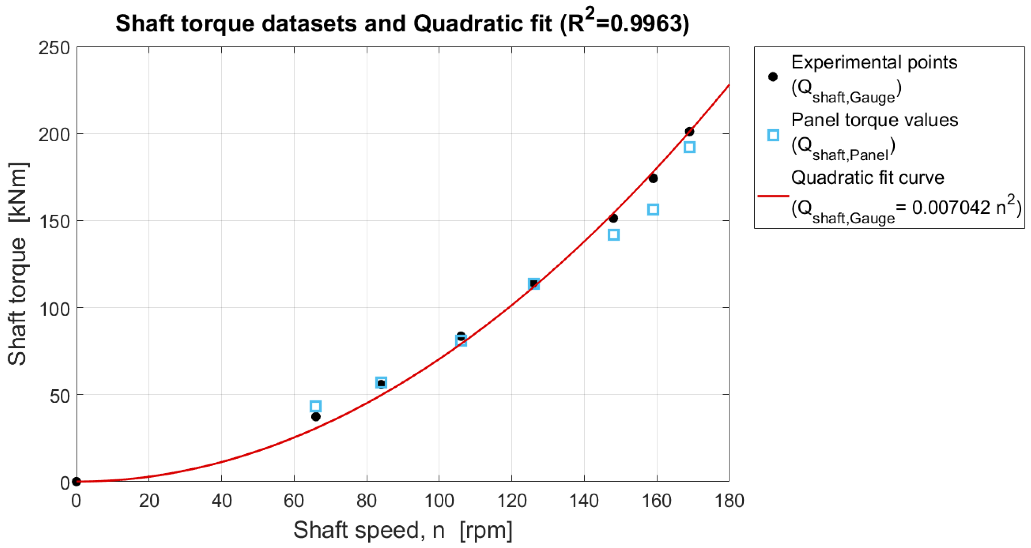
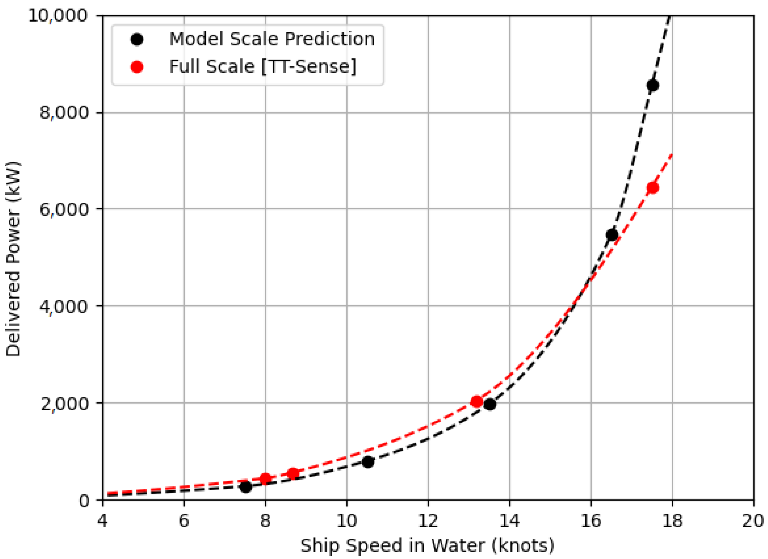
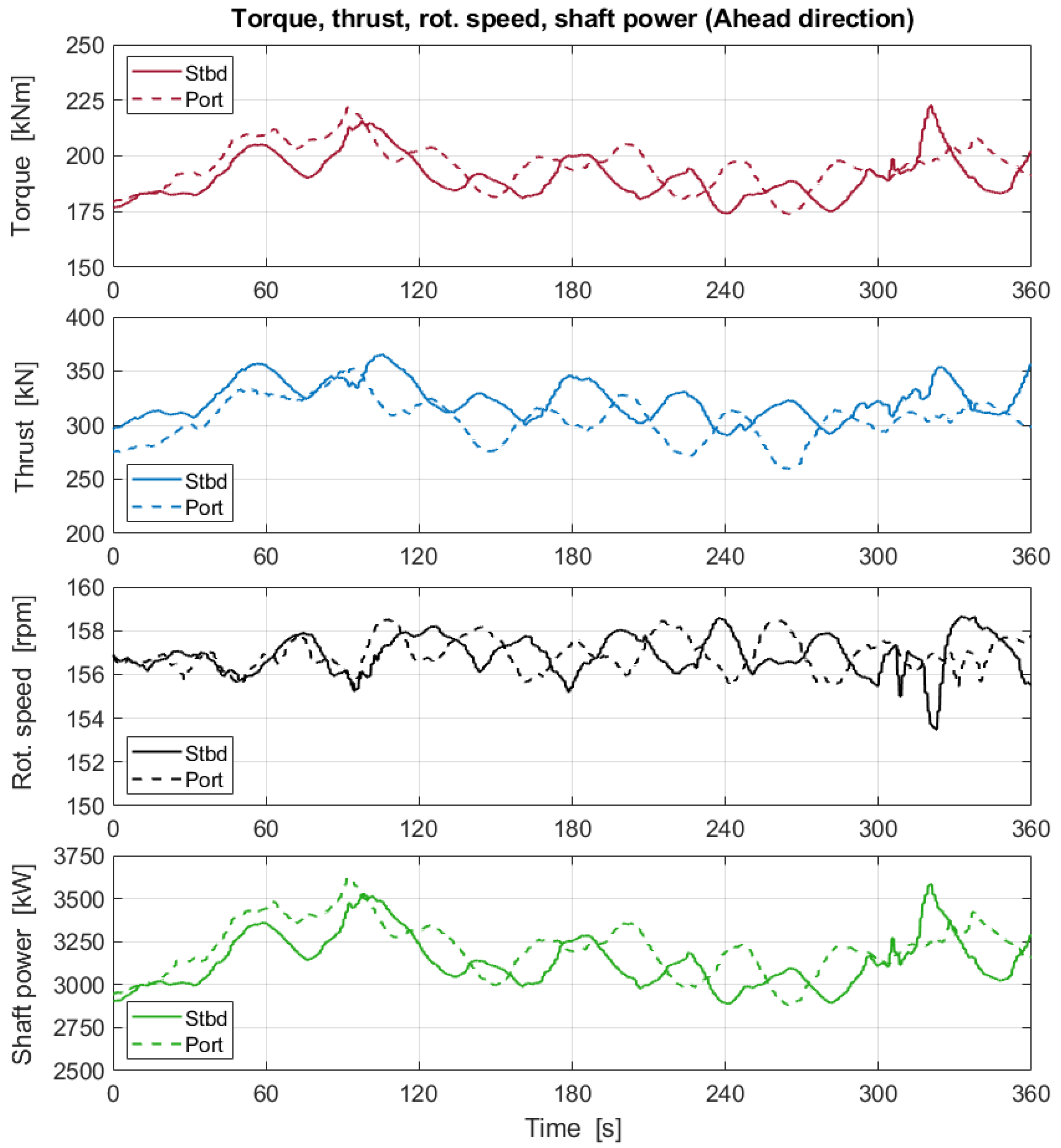
• TT-Sense validation through open water performance data.Figure 13 clearly shows that the TT-Sense device deployed on both shafts provides a sufficiently sensitive estimate of torque and power, which closely match detailed performance estimates via model-scale tests, in uncorrected open-water transits. Additionally, we showed that the dataset produced by the shaft’s optical sensors can be used to validate ship performance predictions during sea ice operations.
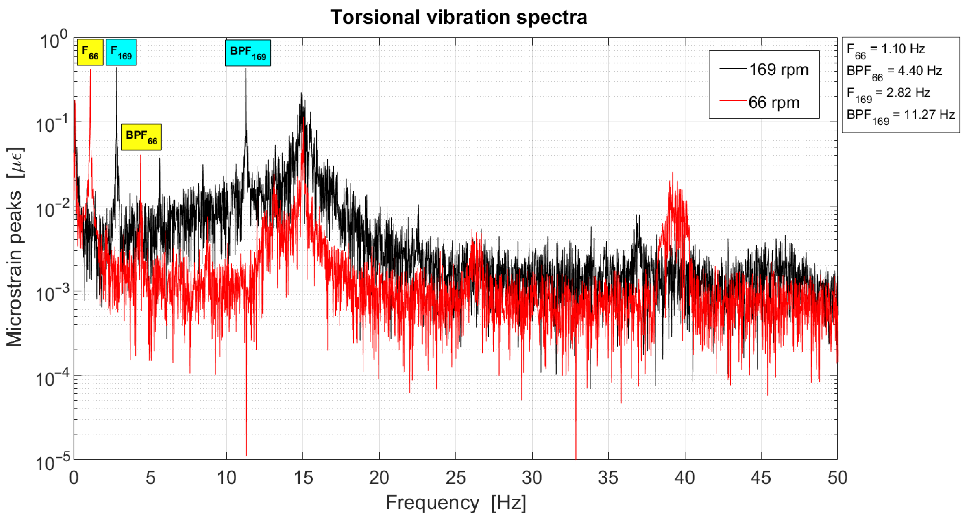
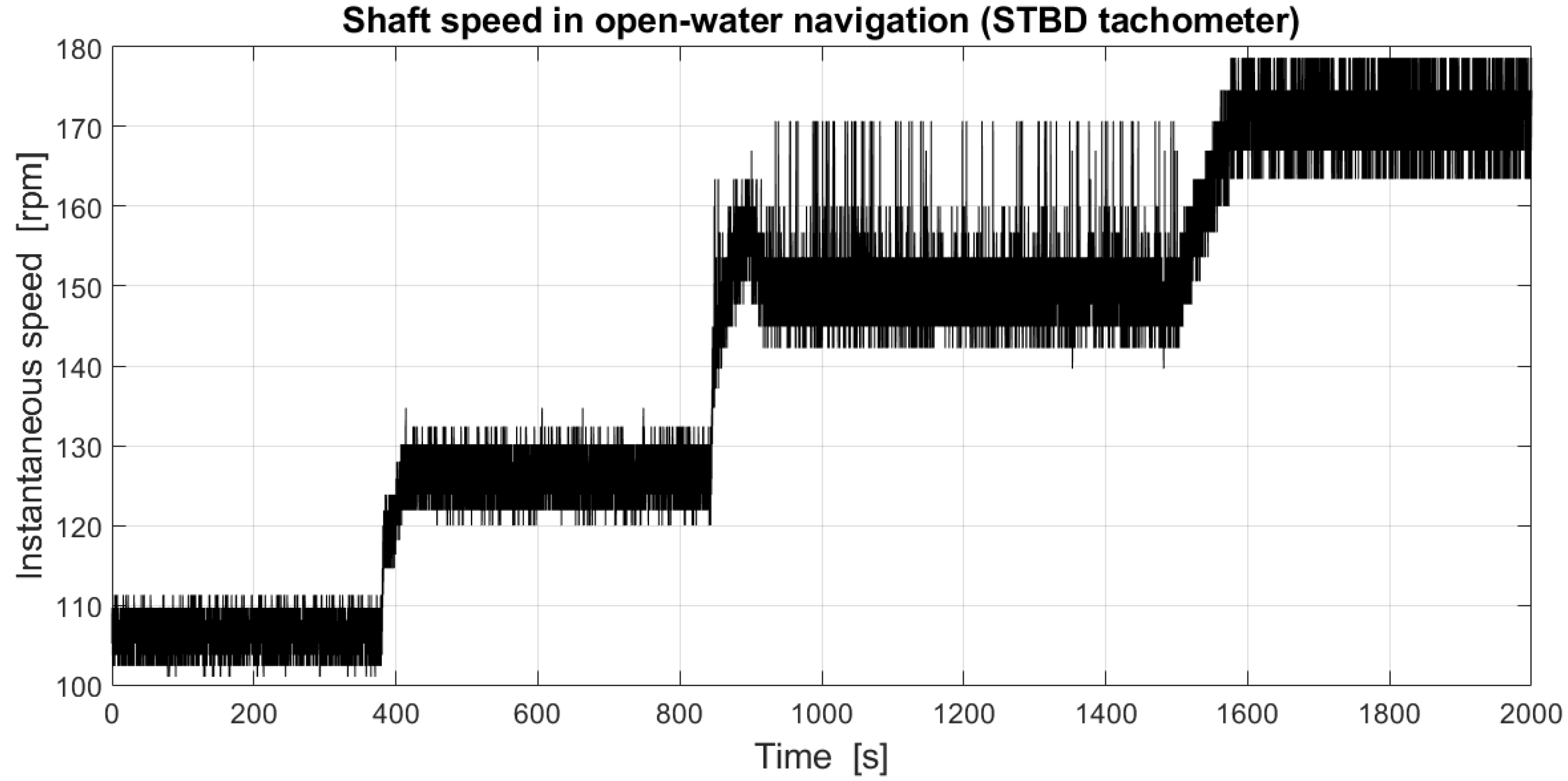
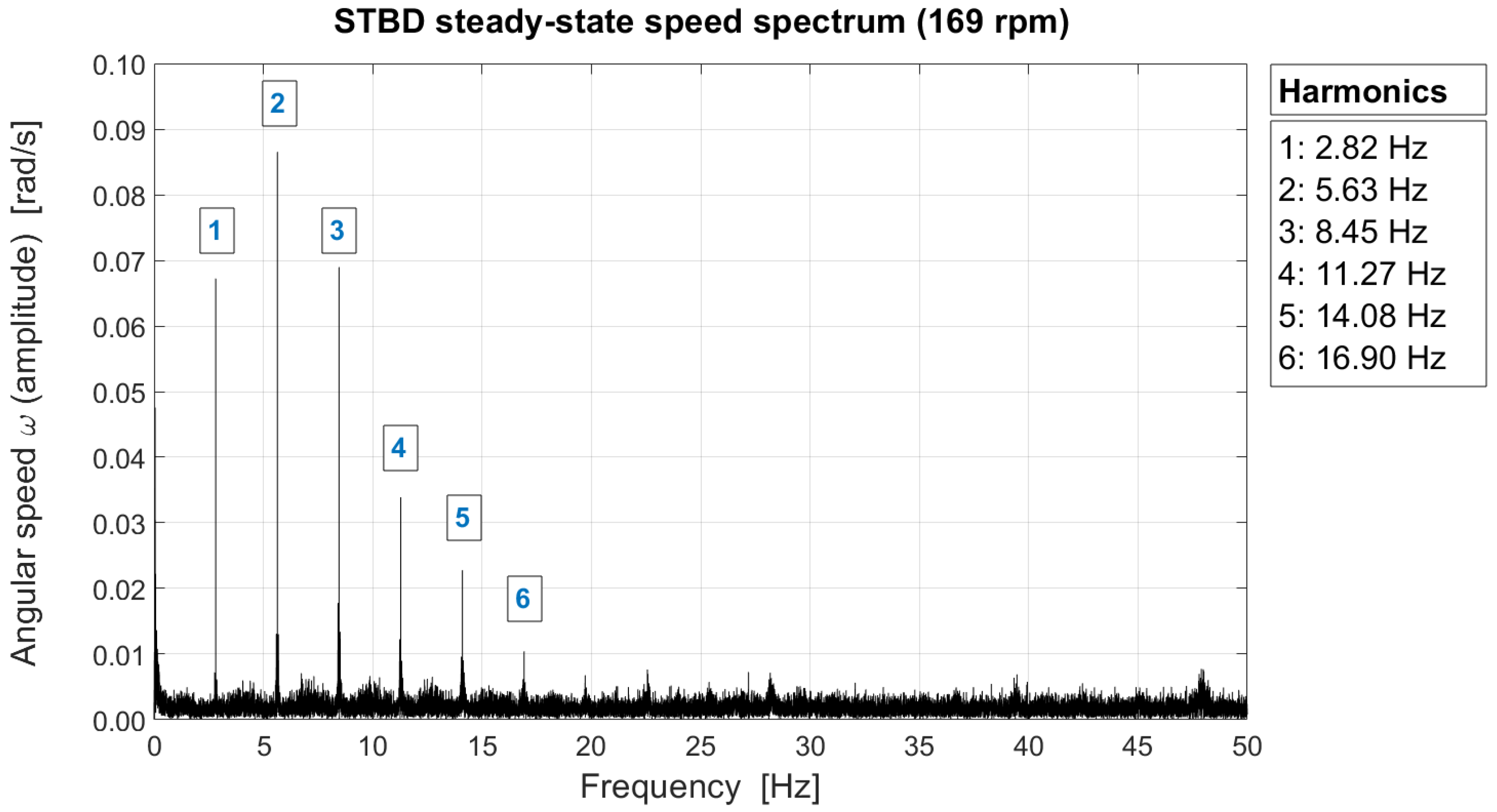
• Tachometer measurements. The dynamic rotational speed measured by the laser sensors allows us to study the torsional vibration response until 50 Hz, which is adequate to represent the major vibration modes of the shaft line and the external excitation spectra. Therefore, resonance events can be detected through these measurements. However, calculating the $\theta \left(f\right)$ spectrum (from $\omega \left(f\right)$) for a single shaft section is insufficient to determine the corresponding shaft torque, which can be obtained through two separate measurements at different sections.
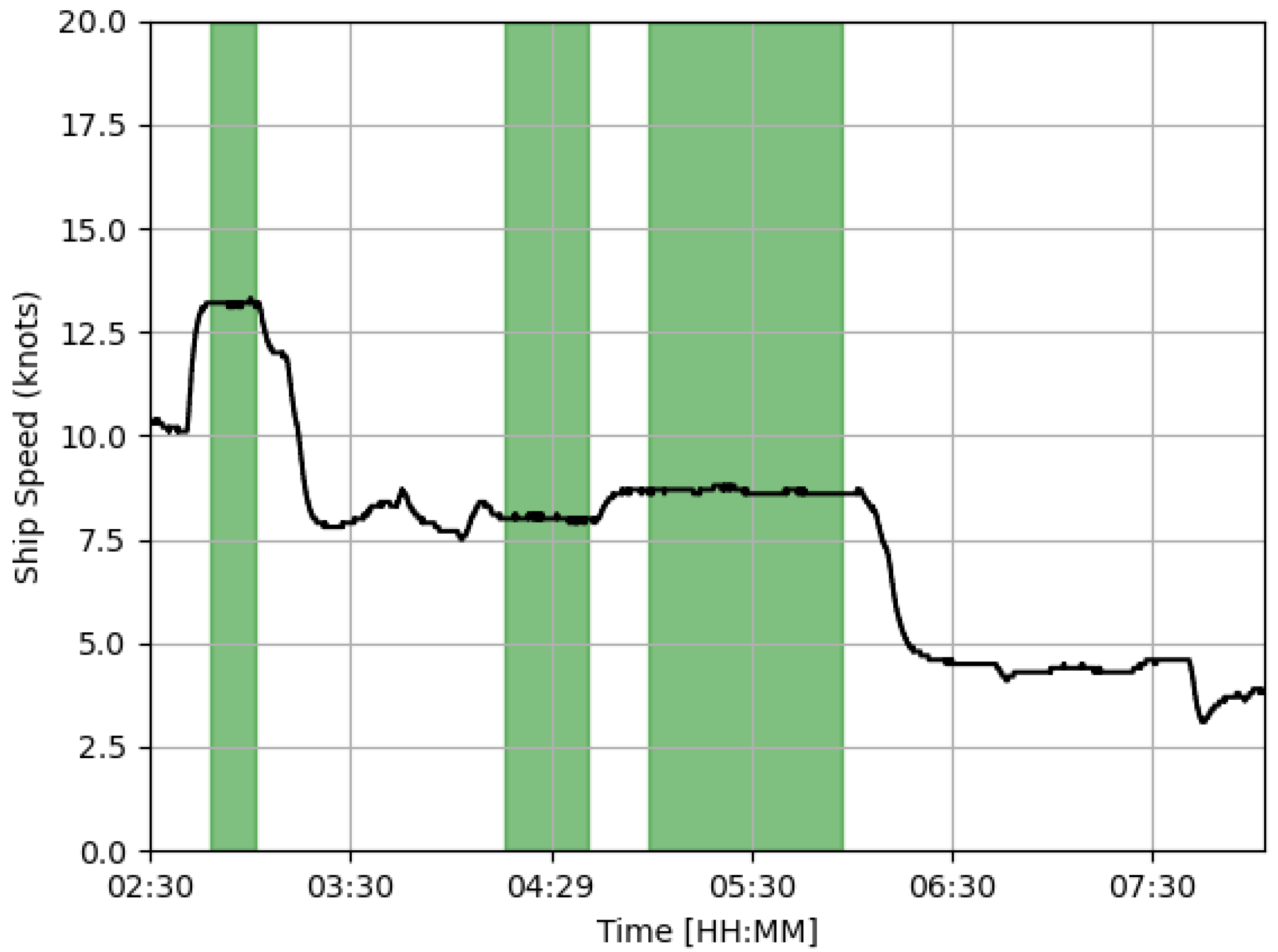
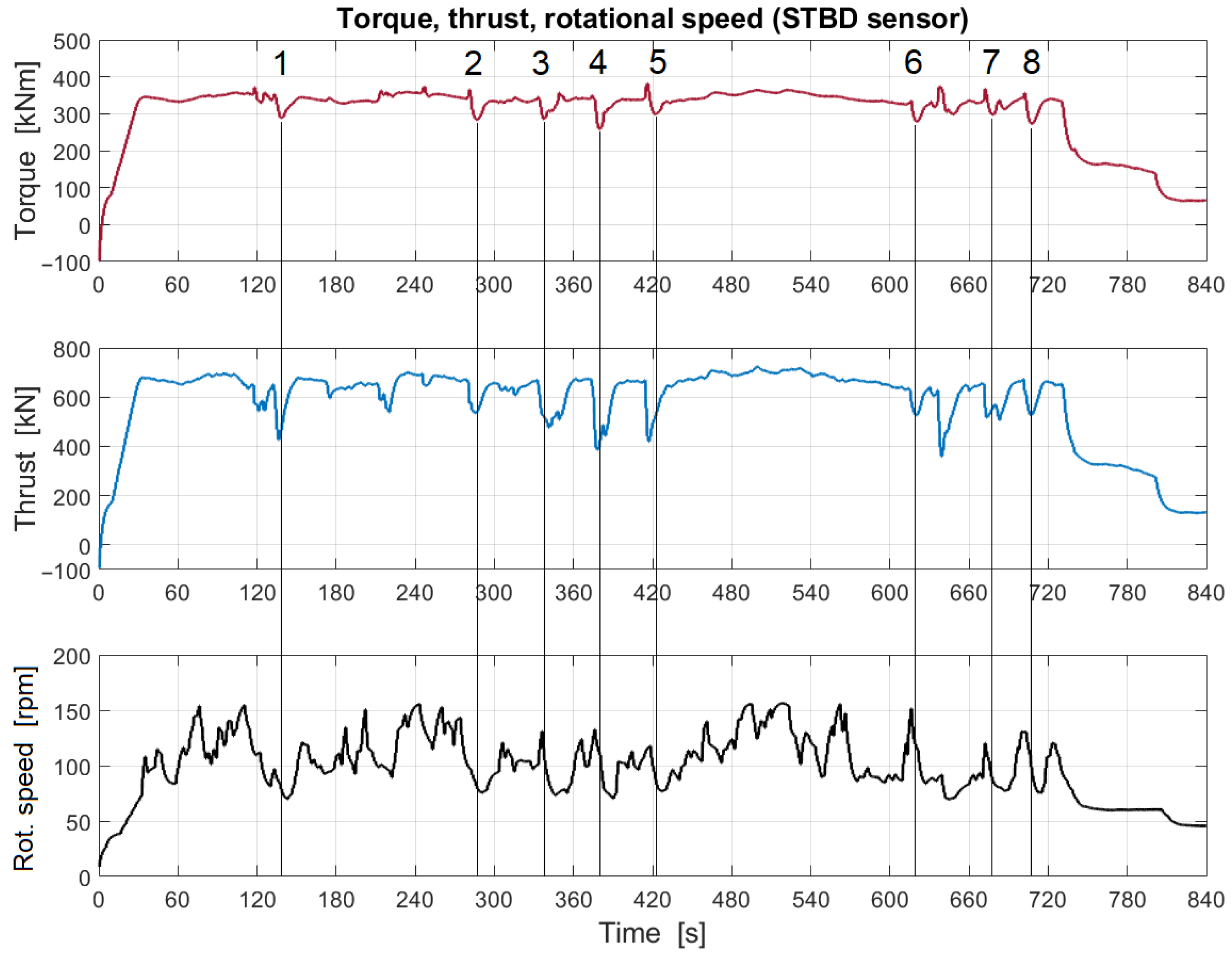
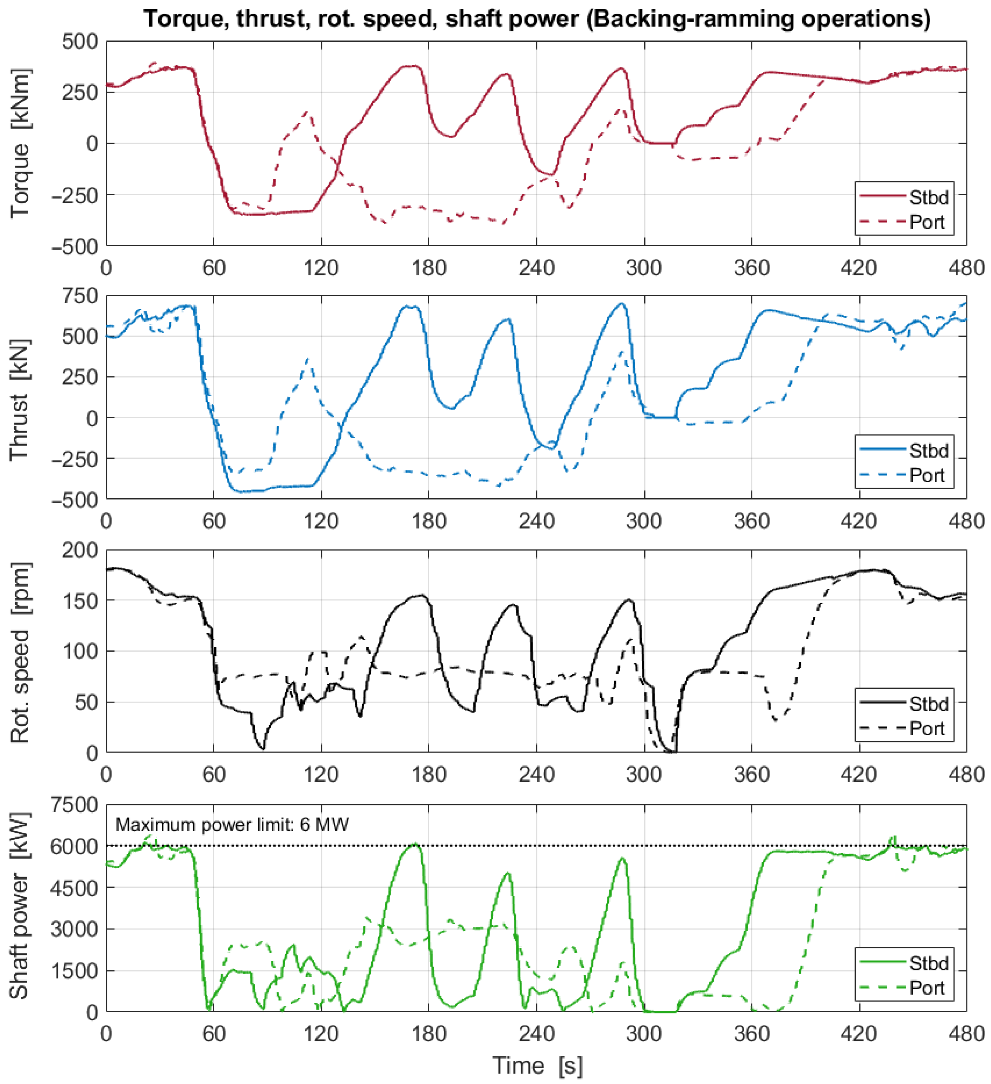
• TT-Sense data in sea ice navigation. The TT-Sense sensors deliver low-frequency shaft thrust and torque perturbations, along with the speed variation. As we can see in Figure 16, Figure 19 and Figure 21, the ice-induced torque amplitude can be evaluated in relation to the corresponding ice conditions. The sampling frequency of 5 Hz represents a limitation of the sensor, as it does not allow us to perform vibration analysis of the shaft’s response. On the other hand, the time tracking of T and Q over long time lapses provides comprehensive monitoring of the propulsion performance and efficiency. The dynamic shafts’ responses—as it can be noticed in Figure 16, Figure 19 and Figure 21—give clear indications on the operation type that the vessel undergoes.
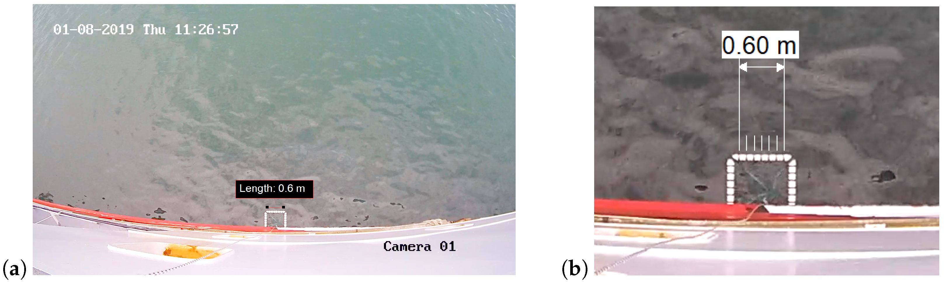
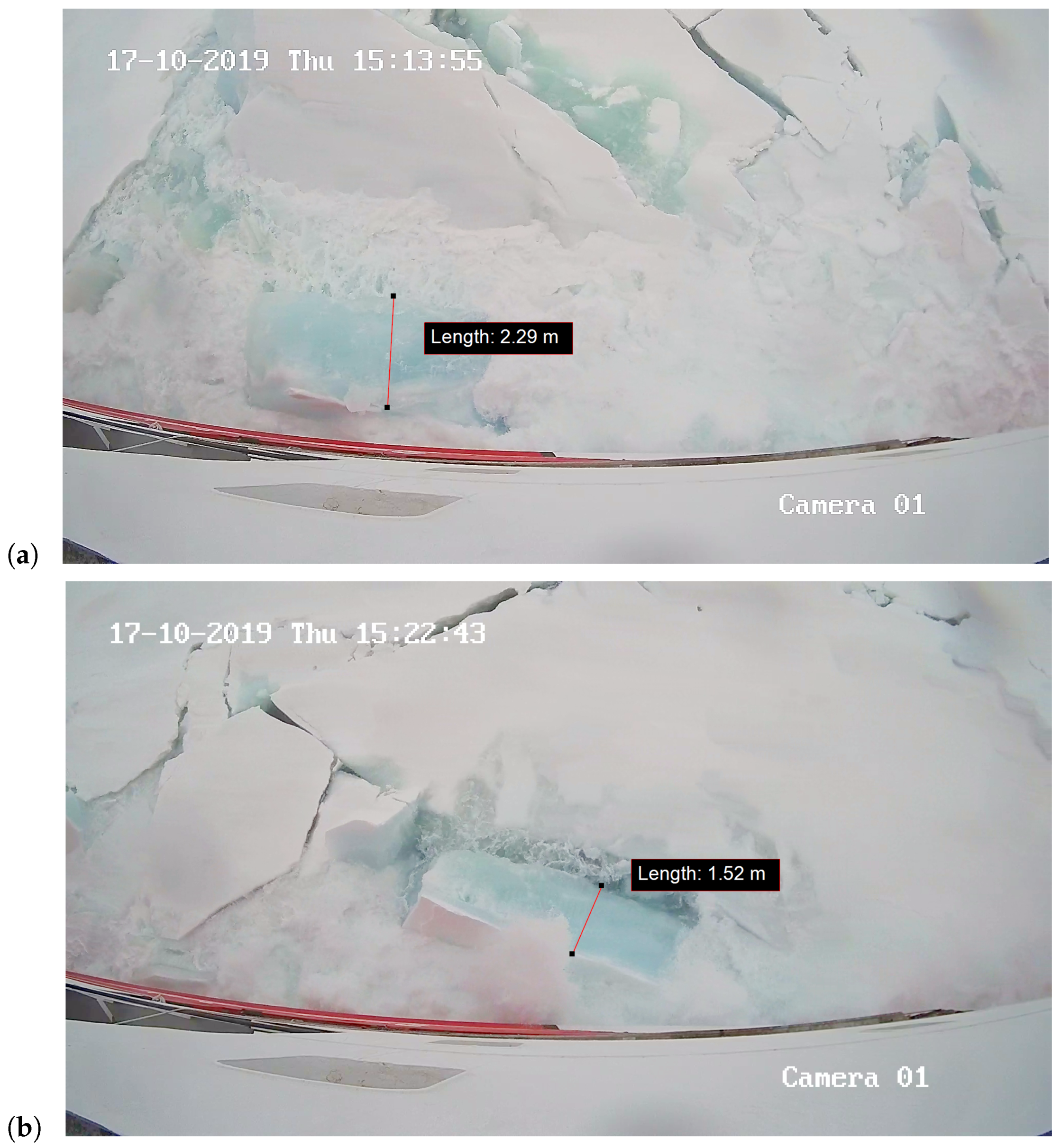
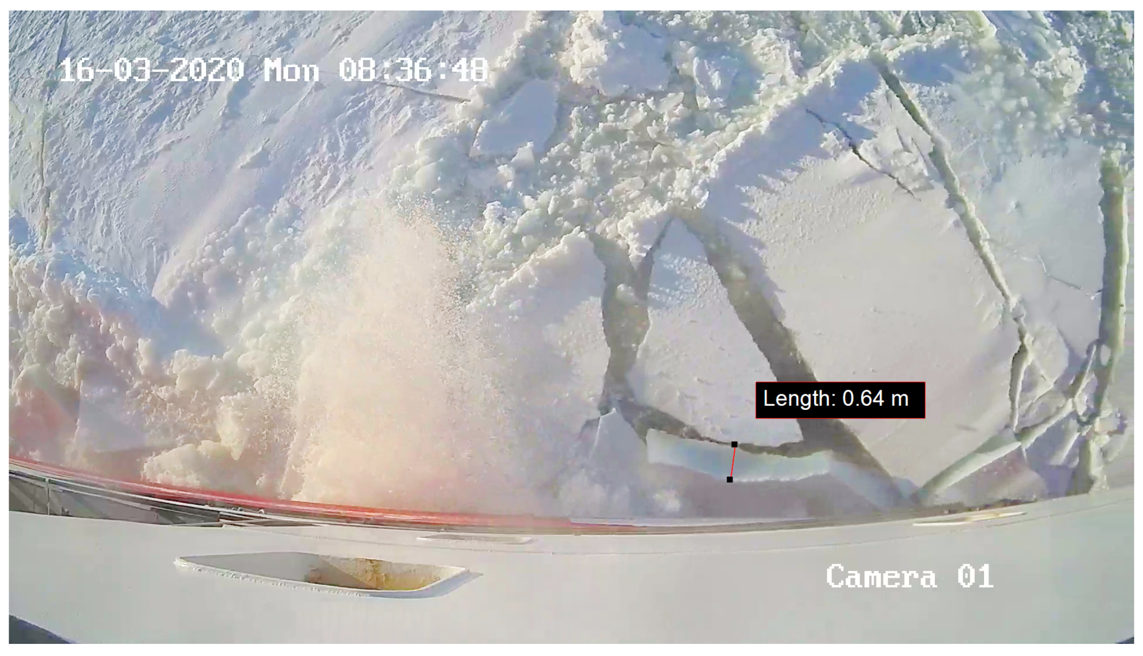
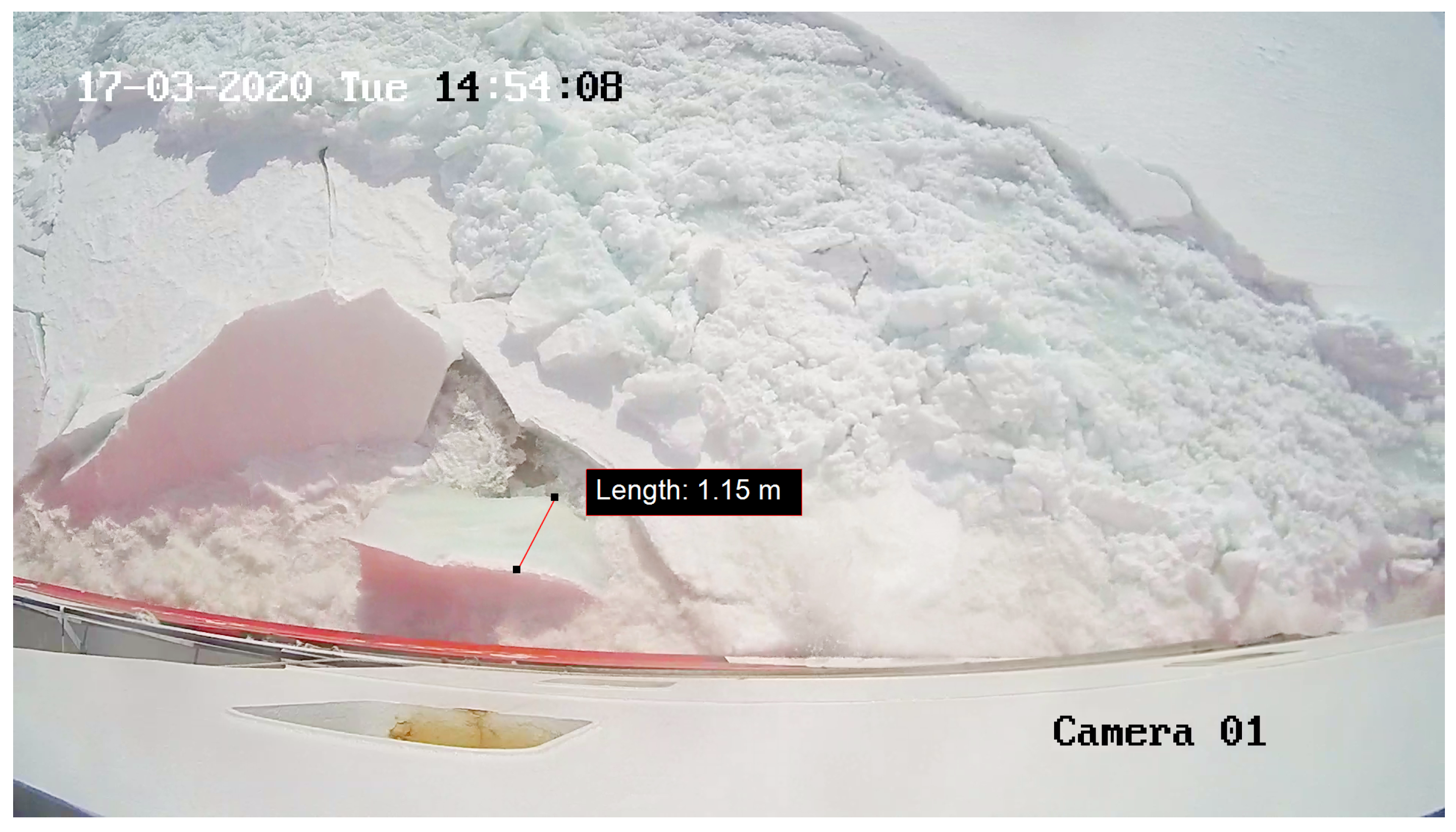
• Sea ice surface video recordings. The ultimate goal of the camera imaging data is to characterize the sea ice conditions in terms of ice pieces’ thickness, as this is the key parameter that determines the ice-propeller torque magnitude in the current Polar Rules [52]. In the time window data considered in Figure 16, the average thickness of the ice floes exceeds 1.5 m, which characterizes that specific ice type as thick first-year ice (Figure 17). Regarding the ice conditions in the March 2020 session (Figure 20 and Figure 22), milder sea ice was encountered. The thickness values of the ice layers determined from the video recordings have been calculated by means of a graphic manipulation software frame by frame (Section 2.4); this procedure may be significantly time-consuming when hundreds of pictures are concerned; therefore, an IA software could be employed to automatically recognize the ice blocks and contour their physical boundaries in the frames.

5. Conclusions

In this paper, we presented a combined measurement system devised to monitor the ship propulsion performance and study the transient torsional behaviour of the shaft lines during icebreaking operations. The system was installed on board the CCG icebreaker Henry Larsen. We showed a preliminary set of results from two expeditions of the vessel: first, open-water torque measurements to validate the optical torque sensor data were introduced; second, we presented a series of experimental data acquired during some icebreaking sessions. The results showed that datasets concerning: (i) shaft thrust; (ii) shaft torque; (iii) shaft speed; (iv) delivered power; (v) torsional vibration measures; and (vi) sea ice visual recordings could be integrated to provide a concurrent overview of the propulsion system status and the ongoing ice conditions. The instrumentation is going to be continuously employed during the future transit voyages and icebreaking operations of the ship. Large data clusters related to various operating scenarios will be obtained and later analyzed, with the long-term goal to establish how different output quantities are correlated to the sea ice conditions encountered during ice navigation.

The Polar Rules issued by the International Association of Classification Societies (IACS) classify ice-going vessels in levels—to assess ships’ operational capability in ice environments—which constitute the Polar Class (PC) framework. One of the sea-ice properties that is key in characterizing each PC level is the ice layer’s thickness [52]. Hence, the full-scale experimental data obtained through our measurement system is fundamental for two primary purposes: first, to provide ship designers with experimental datasets to be used in future Polar-Class vessel design; second, to validate and possibly update the ice thickness criteria defined in the PC notation system.

References

1. Zhang, Z.; Huisingh, D.; Song, M. Exploitation of trans-Arctic maritime transportation. J. Clean. Prod. 2019, 212, 960–973. [Google Scholar] [CrossRef]
2. Silber, G.K.; Adams, J.D. Vessel Operations in the Arctic, 2015–2017. Front. Mar. Sci. 2019, 6, 573–590. [Google Scholar] [CrossRef]
3. Gascard, J.C.; Riemann-Campe, K.; Gerdes, R.; Schyberg, H.; Randriamampianina, R.; Karcher, M.; Zhang, J.; Rafizadeh, M. Future sea ice conditions and weather forecasts in the Arctic: Implications for Arctic shipping. Ambio 2017, 46, 355–367. [Google Scholar] [CrossRef] [PubMed] [Green Version]
4. Perovich, D.K.; Richter-Menge, J.A. Regional variability in sea ice melt in a changing Arctic. Philos. Trans. R. Soc. A Math. Phys. Eng. Sci. 2015, 373, 20140165. [Google Scholar] [CrossRef] [PubMed]
5. Blaauw, R.J. Oil and gas development and opportunities in the Arctic Ocean. In Environmental Security in the Arctic Ocean; Springer: Berlin/Heidelberg, Germany, 2013; pp. 175–184. [Google Scholar]
6. Bogoyavlensky, V. The Arctic and World Ocean: Current State, Prospects and Challenges of Hydrocarbon Resources Development. In Proceedings of the 21st World Petroleum Congress, Moscow, Russia, 15–19 June 2014. [Google Scholar]
7. Gunnarsson, B. Recent ship traffic and developing shipping trends on the Northern Sea Route—Policy implications for future arctic shipping. Mar. Policy 2021, 124, 104369. [Google Scholar] [CrossRef]
8. Pierre, C.; Olivier, F. Relevance of the Northern Sea Route (NSR) for bulk shipping. Transp. Res. Part A Policy Pract. 2015, 78, 337–346. [Google Scholar] [CrossRef]
9. Zhang, Y.; Meng, Q.; Zhang, L. Is the Northern Sea Route attractive to shipping companies? Some insights from recent ship traffic data. Mar. Policy 2016, 73, 53–60. [Google Scholar] [CrossRef]
10. Melia, N.; Haines, K.; Hawkins, E.; Day, J.J. Towards seasonal Arctic shipping route predictions. Environ. Res. Lett. 2017, 12, 084005. [Google Scholar] [CrossRef]
11. Schröder, C.; Reimer, N.; Jochmann, P. Environmental impact of exhaust emissions by Arctic shipping. Ambio 2017, 46, 400–409. [Google Scholar] [CrossRef] [Green Version]
12. Granier, C.; Niemeier, U.; Jungclaus, J.H.; Emmons, L.; Hess, P.; Lamarque, J.F.; Walters, S.; Brasseur, G.P. Ozone pollution from future ship traffic in the Arctic northern passages. Geophys. Res. Lett. 2006, 33, L13807. [Google Scholar] [CrossRef] [Green Version]
13. Browse, J.; Carslaw, K.S.; Schmidt, A.; Corbett, J.J. Impact of future Arctic shipping on high-latitude black carbon deposition. Geophys. Res. Lett. 2013, 40, 4459–4463. [Google Scholar] [CrossRef] [Green Version]
14. Mjelde, A.; Martinsen, K.; Eide, M.; Endresen, Ø. Environmental accounting for Arctic shipping—A framework building on ship tracking data from satellites. Mar. Pollut. Bull. 2014, 87, 22–28. [Google Scholar] [CrossRef] [PubMed]
15. Gong, W.; Beagley, S.R.; Cousineau, S.; Sassi, M.; Munoz-Alpizar, R.; Ménard, S.; Racine, J.; Zhang, J.; Chen, J.; Morrison, H.; et al. Assessing the impact of shipping emissions on air pollution in the Canadian Arctic and northern regions: Current and future modelled scenarios. Atmos. Chem. Phys. 2018, 18, 16653–16687. [Google Scholar] [CrossRef] [Green Version]
16. Yumashev, D.; van Hussen, K.; Gille, J.; Whiteman, G. Towards a balanced view of Arctic shipping: Estimating economic impacts of emissions from increased traffic on the Northern Sea Route. Clim. Chang. 2017, 143, 143–155. [Google Scholar] [CrossRef] [Green Version]
17. Kitagawa, H. Safety and Regulations of Arctic Shipping. In Proceedings of the Twenty-First International Offshore and Polar Engineering Conference, International Society of Offshore and Polar Engineers, Maui, HI, USA, 19–24 June 2011. [Google Scholar]
18. Pietri, D.; Soule, A.B., IV; Kershner, J.; Soles, P.; Sullivan, M. The Arctic shipping and environmental management agreement: A regime for marine pollution. Coast. Manag. 2008, 36, 508–523. [Google Scholar] [CrossRef]
19. Hindley, R.J.; Tustin, R.D.; Upcraft, D.S. Environmental protection regulations and requirements for ships for Arctic sea areas. In Proceedings of the RINA International Conference—Design and Construction of Vessels Operating in Low Temperature Environments, Glasgow, UK, 29–30 November 2017; pp. 107–118. [Google Scholar]
20. Lee, S.K. Rational approach to integrate the design of propulsion power and propeller strength for ice ships. In Proceedings of the 2006 SNAME ICETECH Conference, Banff, AB, Canada, 16–19 July 2006. [Google Scholar]
21. Polić, D.; Ehlers, S.; Æsøy, V.; Pedersen, E. Propulsion Machinery Operating In Ice-A Modelling And Simulation Approach. In Proceedings of the 27th European Conference on Modelling and Simulation (ECMS 2013), Ålesund, Norway, 27–30 May 2013; pp. 191–197. [Google Scholar]
22. Yang, B.; Sun, Z.; Zhang, G.; Wang, Q.; Zong, Z.; Li, Z. Numerical estimation of ship resistance in broken ice and investigation on the effect of floe geometry. Mar. Struct. 2021, 75, 102867. [Google Scholar] [CrossRef]
23. Bose, N.; Veitch, B.; Doucet, J.M. A design approach for ice class propellers. SNAME Trans. 1998, 106, 185–211. [Google Scholar]
24. Vizentin, G.; Vukelic, G.; Murawski, L.; Recho, N.; Orovic, J. Marine propulsion system failures—A review. J. Mar. Sci. Eng. 2020, 8, 662. [Google Scholar] [CrossRef]
25. Norhamo, L.; Bakken, G.M.; Deinboll, O.; Iseskär, J.J. Challenges related to propulsor—Ice interaction in arctic waters. In Proceedings of the First International Symposium on Marine Propulsors (SMP09), Trondheim, Norway, 22–24 June 2009. [Google Scholar]
26. Brouwer, J.; Hagesteijn, G.; Bosman, R. Propeller-ice impacts measurements with a six-component blade load sensor. In Proceedings of the Third International Symposium on Marine Propulsors (SMP13), Launceston, Australia, 5–8 May 2013. [Google Scholar]
27. Khan, A.G.; Hisette, Q.; Streckwall, H.; Liu, P. Numerical investigation of propeller-ice interaction effects. Ocean Eng. 2020, 216, 107716. [Google Scholar] [CrossRef]
28. Xu, P.; Wang, C.; Ye, L.; Guo, C.; Xiong, W.; Wu, S. Cavitation and Induced Excitation Force of Ice-Class Propeller Blocked by Ice. J. Mar. Sci. Eng. 2021, 9, 674. [Google Scholar] [CrossRef]
29. Wang, J.; Akinturk, A.; Bose, N. Numerical prediction of model podded propeller-ice interaction loads. In Proceedings of the 25th International Conference on Offshore Mechanics and Arctic Engineering (OMAE2006), Hamburg, Germany, 4–9 June 2006; pp. 667–674. [Google Scholar]
30. Williams, F.M.; Spender, D.; Mathews, S.T.; Bayly, I. Full Scale Trials in Level Ice with Canadian R-Class Icebreaker. SNAME Trans. 1992, 100, 293–313. [Google Scholar]
31. Suominen, M.; Karhunen, J.; Bekker, A.; Kujala, P.; Elo, M.; Enlund, H.; Saarinen, S. Full-scale measurements on board PSRV SA Agulhas II in the Baltic Sea. In Proceedings of the International Conference on Port and Ocean Engineering Under Arctic Conditions, Espoo, Finland, 9–13 June 2013. [Google Scholar]
32. Suominen, M.; Li, F.; Lu, L.; Kujala, P.; Bekker, A.; Lehtiranta, J. Effect of maneuvering on ice-induced loading on ship hull: Dedicated full-scale tests in the Baltic Sea. J. Mar. Sci. Eng. 2020, 8, 759. [Google Scholar] [CrossRef]
33. Dahler, G.; Stubbs, J.T.; Norhamo, L. Propulsion in ice—Big ships. In Proceedings of the International Conference and Exhibition on Performance of Ship and Structure in Ice—ICETECH, Anchorage, AK, USA, 20–23 September 2010. [Google Scholar]
34. Jussila, M.; Koskinen, P. Ice loads on CP-propeller and propeller shaft of small ferry and their statistical distributions during winter ’87. In Proceedings of the 8th International Conference on Offshore Mechanics and Arctic Engineering, The Hague, The Netherlands, 19–23 March 1989; Volume IV. [Google Scholar]
35. Lensu, M.; Kujala, P.; Kulovesi, J.; Lehtiranta, J.; Suominen, M. Measurements of Antarctic sea ice thickness during the ice transit of SA Agulhas II. In Proceedings of the International Conference on Port and Ocean Engineering Under Arctic Conditions (POAC 2015), Trondheim, Norway, 14–18 June 2015. [Google Scholar]
36. Weissling, B.; Ackley, S.; Wagner, P.; Xie, H. EISCAM—Digital image acquisition and processing for sea ice parameters from ships. Cold Reg. Sci. Technol. 2009, 57, 49–60. [Google Scholar] [CrossRef]
37. Niioka, T.; Kohei, C. Sea ice thickness measurement from an ice breaker using a stereo imaging system consisted of a pairs of high definition video cameras. Int. Arch. Photogramm. Remote Sens. Spat. Inf. Sci. Kyoto Jpn. 2010, 38, 1053–1056. [Google Scholar]
38. Lu, W.; Zhang, Q.; Lubbad, R.; Løset, S.; Skjetne, R. A shipborne measurement system to acquire sea ice thickness and concentration at engineering scale. In Proceedings of the Arctic Technology Conference, St. John’s, NL, Canada, 24–26 October 2016. [Google Scholar]
39. De Waal, R.J.O.; Bekker, A.; Heyns, P.S. Indirect load case estimation for propeller-ice moments from shaft line torque measurements. Cold Reg. Sci. Technol. 2018, 151, 237–248. [Google Scholar] [CrossRef] [Green Version]
40. Suominen, M.; Bekker, A.; Kujala, P.; Soal, K.; Lensu, M. Visual Anctartic Sea Ice Condition Observations during Austral Summers 2012–2016. In Proceedings of the 24th International Conference on Port and Ocean Engineering under Arctic Conditions (POAC 2017), Busan, Korea, 11–16 June 2017. [Google Scholar]
41. de Waal, R.J.O.; Bekker, A.; Heyns, P.S. Bi-Polar Full Scale Measurements of Operational Loading on Polar Vessel Shaft-lines. In Proceedings of the 24th International Conference on Port and Ocean Engineering under Arctic Conditions (POAC 2017), Busan, Korea, 11–16 June 2017. [Google Scholar]
42. Ikonen, T.; Peltokorpi, O.; Karhunen, J. Inverse ice-induced moment determination on the propeller of an ice-going vessel. Cold Reg. Sci. Technol. 2015, 112, 1–13. [Google Scholar] [CrossRef]
43. Nickerson, B.M.; Bekker, A. Inverse model for the estimation of ice-induced propeller moments using modal superposition. Appl. Math. Model. 2022, 102, 640–660. [Google Scholar] [CrossRef]
44. Remond, D. Practical performances of high-speed measurement of gear transmission error or torsional vibrations with optical encoders. Meas. Sci. Technol. 1998, 9, 347. [Google Scholar] [CrossRef]
45. Burella, G.; Moro, L.; Oldford, D. Analysis and validation of a procedure for a lumped model of Polar Class ship shafting systems for transient torsional vibrations. J. Mar. Sci. Technol. 2018, 23, 633–646. [Google Scholar] [CrossRef]
46. Burella, G.; Moro, L. Transient torsional analysis of polar class vessel shafting systems using a lumped model and finite element analysis. In Proceedings of the 27th International Ocean and Polar Engineering Conference, San Francisco, CA, USA, 25–30 June 2017. [Google Scholar]
47. Zambon, A.; Moro, L. Torsional vibration analysis of diesel driven propulsion systems: The case of a polar-class vessel. Ocean Eng. 2022, 245, 110330. [Google Scholar] [CrossRef]
48. Hoffmann, K. Applying the Wheatstone Bridge Circuit; Version W1569en-1.0; Technical Report; Hottinger Baldwin Messtechnik (HBM) GmbH: Darmstadt, Germany, 2001. [Google Scholar]
49. MAN. Basic Principles of Ship Propulsion; MAN Diesel & Turbo: Frederikshavn, Denmark, 2011. [Google Scholar]
50. Carlton, J.S. Marine Propellers and Propulsion, 2nd ed.; Butterworth-Heinemann, Elsevier: Amsterdam, The Netherlands, 2007. [Google Scholar]
51. Wang, J. CCG’s Baseline Model Tests Using Henry Larsen Icebreaker [NRC-OCRE-2021-TR-004]; Technical Report; National Research Council of Canada–Ocean, Coastal and River Engineering (NRC-OCRE): St. John’s, NL, Canada, 2021. [Google Scholar]
52. International Association of Classification Societies (IACS). Requirements Concerning Polar Class—Polar Rules; International Association of Classification Societies (IACS): London, UK, 2006; Rev. 1 January 2007, Corr. 1 October 2007. [Google Scholar]
Figure 1. Layout map of the measurement system installed on board CCGS Henry Larsen.
Jmse 10 00522 g001
Figure 2. Shaft instrumentation installed on the Starboard shaftline of CCGS Henry Larsen.
Jmse 10 00522 g002
Figure 3. TT-Sense ® sensor: cross-section drawing (a); accommodation on the Starboard shaft (b).
Jmse 10 00522 g003
Figure 4. Brüel & Kjær Type 2981 laser tachometer (a); accommodation on the Starboard shaft (b).
Jmse 10 00522 g004
Figure 5. Railing support and positioning of the camera (a); view angle on the sea surface (b).
Jmse 10 00522 g005
Figure 6. Floating frame for the calibration procedure: camera frame (a); zoomed view (b).
Jmse 10 00522 g006
Figure 7. Arrangement of the shaft equipment (a); instrumentation attached to the shaft (b).
Jmse 10 00522 g007
Figure 8. Route on 17–18 October 2019: larger view (a) and zoomed view (b) (via Google Earth ® ).
Jmse 10 00522 g008
Figure 9. Route on 15–18 March 2020: larger view (a) and zoomed view (b) (via Google Earth ® ).
Jmse 10 00522 g009
Figure 10. Torsional vibration spectra at 66 rpm and 169 rpm.
Jmse 10 00522 g010
Figure 11. Shaft torque values ( Q shaft , Gauge and Q shaft , Panel ) and fit curve of Q shaft , Gauge ( n ) .
Jmse 10 00522 g011
Figure 12. Open-water longitudinal speed of CCGS Henry Larsen; 2 to 6 a.m., 30 October 2021.
Jmse 10 00522 g012
Figure 13. Comparison of the experimental model-scale [51] and full-scale effective power.
Jmse 10 00522 g013
Figure 14. Shaft speed determined from the tachometer pulse signal under-sampling at 100 Hz.
Jmse 10 00522 g014
Figure 15. Spectrum of ω ( f ) at n = 169 rpm, in steady-state conditions, at the Starboard-side shaftline.
Jmse 10 00522 g015
Figure 16. Time series of Q, T, and n during forward-direction ice navigation, on 17 October 2019.
Jmse 10 00522 g016
Figure 17. Ice thickness values: two frames corresponding to events 2 (a) and 6 (b) shown in Figure 16.
Jmse 10 00522 g017
Figure 18. Pitch, roll and heave accelerations experienced by the ship during heavy-ice operations on 17 October 2019, in the time window of Figure 16.
Jmse 10 00522 g018
Figure 19. Time series of Q, T, and n during forward-direction ice navigation, on 16 March 2020. The data series of both shafts’ sensors are plotted.
Jmse 10 00522 g019
Figure 20. Ice conditions characterizing the time interval of the dataset from Figure 19.
Jmse 10 00522 g020
Figure 21. Time series of Q, T, and n during baking-ramming icebreaking operations, on 17 March 2020. The data series of both shafts’ sensors are plotted.
Jmse 10 00522 g021
Figure 22. Ice conditions characterizing the time interval of the dataset from Figure 21.
Jmse 10 00522 g022
Figure 23. Pitch, roll and heave accelerations of the ship during the icebreaking operations on: (a) 16 March 2020, in the time window of Figure 19; (b) 17 March 2020, in the time window of Figure 21.
Jmse 10 00522 g023