
Performance Simulation of Marine Cycloidal Propellers: A Both Theoretical and Heuristic Approach


1
Department of Industrial Engineering (DII), University of Naples Federico II, 80138 Napoli, Italy
2
Department of Electrical, Electronics and Telecommunication Engineering and Naval Architecture (DITEN), University of Genoa, 16145 Genoa, Italy
3
Department of Mechanical, Energy, Management and Transport Engineering (DIME), University of Genoa, 16145 Genoa, Italy
*
Author to whom correspondence should be addressed.
†
These authors contributed equally to this work.
J. Mar. Sci. Eng. 2022, 10(4), 505; https://doi.org/10.3390/jmse10040505
Submission received: 15 February 2022
/
Revised: 25 March 2022
/
Accepted: 29 March 2022
/
Published: 6 April 2022
(This article belongs to the Special Issue Smart Control of Ship Propulsion System)
Abstract
:The importance of mathematical and numerical simulation in marine engineering is growing together with the complexity of the designed systems. In general, simulation a makes it possible to improve the engineering design, reducing working time and costs of production as well. In this respect, the implementation of a simulation model for cycloidal propellers is presented. Cycloidal thrusters are being increasingly used in marine applications. Their best performance concerns low-speed applications, due to their ability to steer thrust in any direction. The proposed simulator is able to assess the performance of cycloidal propellers in terms of the generated thrust and torque, without resorting to consuming and demanding computational tools, such as CFD methods. This feature makes the presented model particularly suitable for the simulation in the time domain of the maneuverability of surface units, equipped with cycloidal propellers. In this regard, after embodying the implemented model in an already existing simulation platform for maneuverability, we show the most significant outputs concerning some simulated maneuvers, performed at cruise speed.
1. Introduction
Until the past century, the only way that naval architects had to predict the behavior of the system (intended as the ship or a part of it, such as the propulsion plant, or the auxiliary systems) they were working on, was to build a prototype and test it. Nowadays, thanks to the development and the progress of computer science, it is possible to shape not prototypes but simulators, based on mathematical laws, that can predict in advance the behavior not only of a single subsystem, but also of the whole ship. Indeed, one of the main advantages of mathematical and numerical simulation is the possibility to compare different design choices, so improving the engineering design and reducing working time and costs as well.
For example, making use of mathematical models, the hull performance can be analyzed under any weather conditions [1,2,3], it is possible to assess whether the designed machinery can guarantee the needed power [4], the magnitude and the direction of propulsion and steering forces can be predicted [5,6], or any kind of failure conditions can be analyzed [7,8,9].
Among the several thruster types, cycloidal propellers (CPs) are widely used on water tractors, ferries and some naval vessels. CPs are made of a set of vertical blade protruding from the hull and performing two main rotations: one around the rotor axis and one around the axis passing through the blade pivoting centre. Depending on their eccentricity value e, namely the ratio between the distance of the steering centre from the propeller axis and the radius of the rotor, they can be classified into true cycloidal (), epicycloidal () and trochoidal propellers (). Being able to generate almost the same thrust in every direction and combine both thrust and steering in a singel unit, CPs are very suitable for low-speed applications, such as dynamic positioning operations for instance.
To date, some investigations have been performed in order to model the behavior of such devices. In [10,11,12,13], some performances of cycloidal rudders have been shown, while propeller–hull interactions have been presented in [14], mainly in connection with maneuverability aspects. In this paper, the main features of a time domain simulation model for CPs are presented. The model is developed on a Matlab©Simulink platform and is able to calculate the time histories of the provided thrust and torque. The implemented model relies on a mixture of theoretical and empirical considerations. In particular, the propeller thrust and torque evaluation is based on the kinematics of each single blade, taking into account suitable correction factors in order to properly consider “dissipative” phenomena (such as interference between blades, the shielding induced by the half of the rotor which receives the oncoming flow, and the slight reduction of back thrust). The calibration of the simulator is carried out by comparing simulation outputs with real data found in open source. The final result is a simulation platform able to predict the performance of a CP in terms of generated thrust and torque, avoiding consuming and demanding computations, such as CFD methods. This is one of the significant aspects of the developed simulator that makes its use really effective when integrated into a platform for the simulation of ship motions.
In this regard, a first application of the developed simulator has been the validation of different thrust allocation logics of a DP system for a surface vessel equipped with a bow thruster and two cycloidal propellers at stern [15,16]. After that, in order to assess the reliability of the obtained simulation model, some maneuvers at cruise speed have been performed, embodying the CP simulator into a more complex dynamic model for maneuverability. In the following, the simulation outputs for one of these maneuvers are presented.
2. The Simulation Platform
As mentioned above, the present work is based on the simulation model which has been presented in [17,18] and concerns a 80 m long patrol vessel from the Italian Coast Guard. Such a simulation platform has been developed modular in order to be able to dealt with and possibly replace separately different sub-systems.
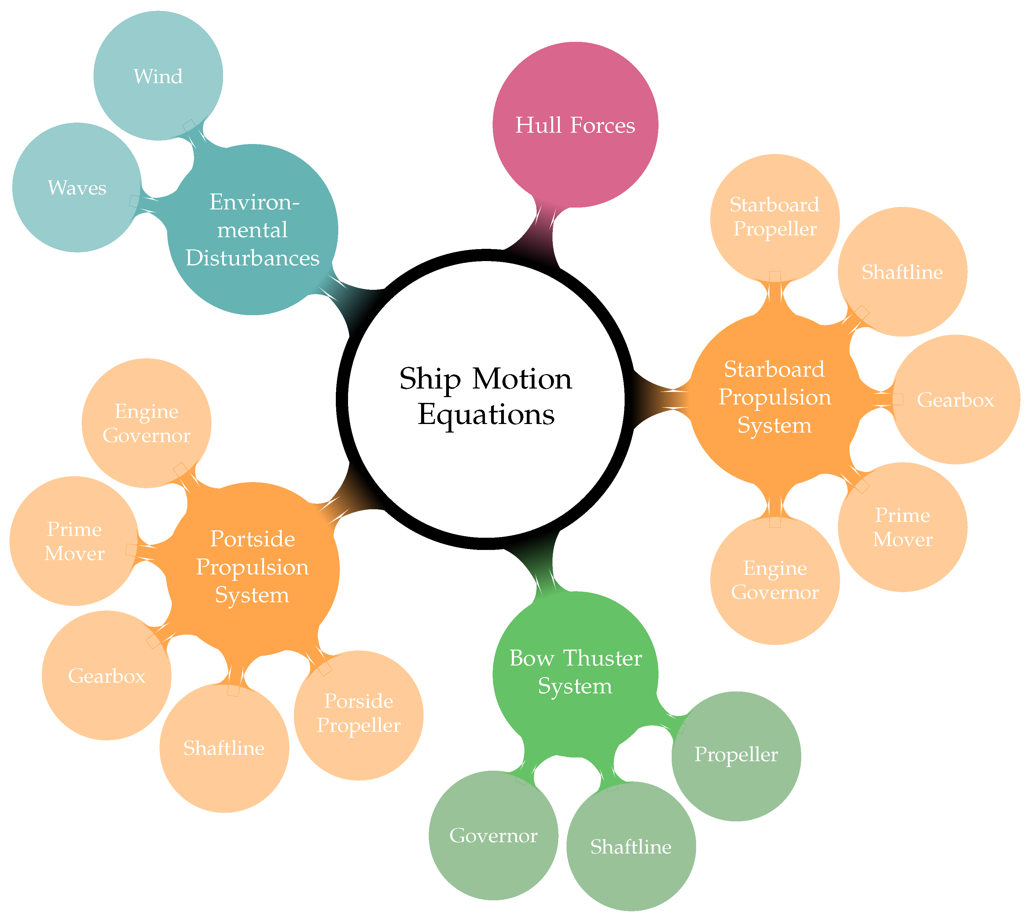
In modeling vessel dynamics, a crucial aspect is developing suitable mathematical models that reproduce the forces acting on the ship, as accurately as possible. In such a process, a complex system of coupled time-domain equations determines the evolution in time of each quantity which contributes to the ship dynamics. Usually, simulation platform are represented by means of flow–charts. In this work, the modular concept of the adopted platform is described by the mind map drawn in Figure 1, where the main part is represented by the motion equations of the ship (1) that mutually interact with the other sub-systems describing all the forces acting on the ship itself. Such forces mainly concern the interaction of the hull with the propulsion and steering systems as well as the environmental disturbs.
Whenever dealing with maneuvering problems, it is common to introduce two reference frames: the Earth-fixed reference frame and the body-fixed frame . Choosing the origin O as located on the mean water-free surface at midship, the main equations governing the ship motion are expressed as
where denotes the linear velocity of O expressed in the body-fixed basis and is the angular velocity, is the vessel displacement, is the longitudinal coordinate of gravity center w.r.t. , is the vessel mass, is the moment of inertia about -axis, and are the resultants of forces and the moments expressed in the -basis, respectively. In addition, , , , where subscripts H, P, and E refer to hull, propellers, and environmental forces and moments respectively.
3. Cycloidal Propeller Model
Cycloidal propellers allows precise and stepless thrust generation since propulsion and steering forces can be generated and varied simultaneously. As a result of the rotation around its vertical axis, the same amount of thrust can be provided almost over by blades with hydrodynamically shaped profiles that assure a high degree of efficiency. In this section, a detailed description of the mathematical model developed for the computation of the thrust T and the torque delivered by a CP is presented.
3.1. Blade Motion
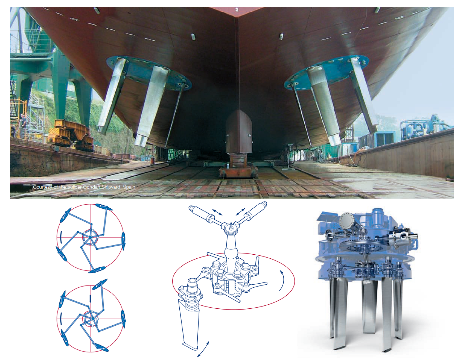
The rapid and precise thrust variation of CPs is based on the kinematics of the blades (usually from 4 to 6 and equally spaced from each other) that move along a circular path, centered at the rotor center, and at the same time perform a superimposed pivoting motion around a suitable vertical axis. When the steering center overlaps the center of the rotor casing, the blades are not angled with respect to the tangent to the blade circular trajectory and no thrust is originated in this circumstance. Instead, if the steering center is moved away from the center of the rotor casing, the blades are set at a variable angle with respect to the tangent of their circular path, and thrust is generated. From top to bottom, Figure 2 shows an example of the installation of two CPs on a ship, with some details of the machinery. During the revolution motion, the maximum angle reached by the blades increases with the eccentricity e, defined as:
where is the distance between the center of the rotor O and the steering center C, and is the radius of the rotor. The motion of the pivot point (assumed as the center of mass) of the blade, relative to a stationary observer, results from the superimposition of the rotational movement of the rotor casing along a straight line representing the forward motion of the vessel. The pivot point follows the curve of a cycloid. The rolling radius of the cycloid is and the advance coefficient is:
where is the advance velocity and n is the rotor speed. During one revolution, the propeller travels a distance in the direction of the vessel motion.
To generate thrust, the blades are angled with respect to the circular path described by their pivoting point. To achieve this, the steering center is moved from O to C. The resulting angle of attack leads to the generation of hydrodynamic lift and drag forces on each blade. The thrust provided by the propeller is the sum of such hydrodynamic forces, is always perpendicular to the line and its intensity increases with the distance . By shifting the steering center C, it is possible to produce thrust in any direction and of different intensities. Therefore, the thrust provided by an epicycloidal propeller can be represented as a function of two plane polar coordinates:
- the geometric or driving pitch (between 0 and for constructive limits): that is the distance (expressed as a percentage of the rotor radius ) between the steering center C and the center of the rotor O;
- the steering pitch (between and ): the angle between a fixed axis (with respect to the hull) and the line .
3.2. Thrust Generation
Changing the steering center, the blades acquire a certain attack angle, so generating corresponding lift and drag forces which give rise to the desired thrust. The hydrodynamic forces components acting transversely to the desired thrust direction cancel each other out. It is possible to produce thrust in any direction putting the steering center in the right position. The zero-thrust condition can be selected at any time, making the ship very safe to handle.
Each blade generates instantly a hydrodynamic force which is the sum of the lift (component of the hydrodynamic force, perpendicular to the oncoming flow) and the drag (parallel to the oncoming flow). The sum of all the hydrodynamic forces generated by all the blades gives rise to the corresponding total thrust. Also, each blade generates a corresponding torque which contributes to the total torque acting on the propeller. For each choice of driving and steering pitch, there are corresponding curves of thrust and torque coefficients and as functions of the advance coefficient . The coefficients and are defined in analogy with the corresponding screw-propeller coefficients, respectively and , by the formulae reported in Table 1.
3.3. Kinematics of the Blade
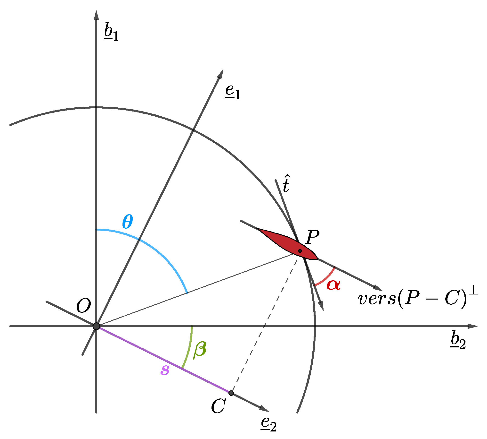
In this section, the kinematical model of a blade is presented. In particular, a dimensional plane model has been adopted, propellers have been modeled as counter-rotating and two distinguished coordinate systems have been introduced: the first one is the hull-fixed frame, while the second one is rotated clockwise, about the vertical axis passing through O and parallel to , by an angle (the steering pitch) which determines (the perpendicular of) the steering force direction. The angle is related to the rudder pitch of the cycloidal propeller. The steering center C lies on the straight line passing through O and parallel to . The relationship between the bases and , in accordance with Figure 3, is expressed as
During the rotation, the projection P of the blade shaft on the plane describes a circumference having center O e radius R coinciding with the rotor radius. Such a circumference is parameterized by
where denotes the angle (function of time) describing the revolution motion of the blade. The unit vector tangent to the circular path of P has components in the vector basis of the form
Introducing the vector
the vector joining the steering center C with the point P can be expressed as
The variable s is usually called driving pitch and controls the magnitude of the thrust. The unit vector orthogonal to and belonging to the plane identifies with the unit vector of the blade chord and it is given by
The pivoting motion of the blade around its own vertical axis can be described by the angle (function of time) between the unit vectors and . Due to the relation
where the dot denotes the usual scalar product between vectors, choosing anticlockwise the positive direction of rotation around the blade shaft, the pivoting angle can be defined as
The above outlined kinematical model can be summarized by the following figure.
Supposing now that the vessel is moving, let be the velocity of O (with respect to an Earth-fixed frame) expressed in the hull-fixed basis. Denoting by
the velocity of the point P with respect to the body-fixed frame, the velocity of P with respect to the Earth-fixed frame is given by
where is the angular velocity of the vessel. The velocity of the oncoming flow experienced at P by a blade-fixed observer is then ; its unit vector is expressed as
Making use of the unit vector it is possible to characterize the attack angle of the incident flow as
3.4. Hydrodynamic Forces
Making use of some simplifying assumptions, a suitable model for evaluating the hydrodynamic forces generated by each blade is presented. It is supposed that the velocity of the incident flow is the same on the entire surface of the blade and coincides with . Under such a condition, the lift and drag produced by each blade can be expressed as
where and are the lift and drag coefficients, respectively; is the sea water density; A is the blade lateral area; is the oncoming flow velocity; is the unit vector of the lift force (unit vector of the oncoming flow at P); and is the unit vector of the drag force (perpendicular to ).
The unit vector can be determined by the following procedure, in which two main scenarios are distinguished:
- the attack angle belongs to the interval , namely the oncoming flow hits the blade from the front. In such a circumstance, the unit vector is determined according to the requirements
- , the oncoming flow hits the blade from the back. In this case, is singled out by the requests:
As remaining particular cases, if or there is no lift while if then . The above described procedure allows us to determine the lift and drag provided by each single blade. The resultant hydrodynamic force generated by the epicycloidal propeller can be computed as the sum of all contributions given by each blade.
3.5. Torque Acting on the Rotor
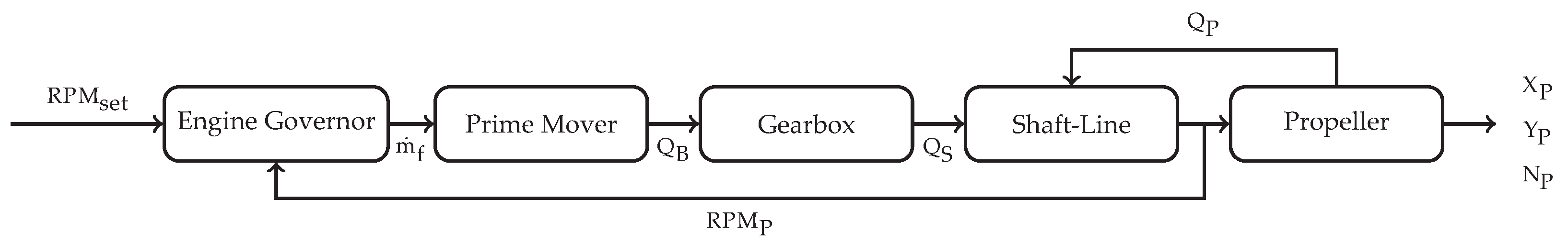
Figure 4 shows the implemented model for the propulsion system. Input data of the model are the desired engine speed , the desired propeller pitch s, and the desired thrust angle . The output is the array composed by the longitudinal and lateral propeller forces and the resulting moment.
The dynamics of the shaft line is described by the equation:
where n is the shaft speed; is the total axial inertia taking into account: (i) engine, (ii) gears, (iii) shaft and (iv) propeller contributions; is the engine torque; represents frictions; and is the propeller torque.
In order to compute the torque acting on the rotor, the Newton-Euler moments equations for each single blade and for the rotor are taken into account separately. Developed in the hull-fixed reference frame and with respect to the point O (center of the rotor), the Newton-Euler moments equation for each blade can be expressed as
where , , , and are the moments acting on the blade, respectively due to hydrodynamic, weight, reactive and inertial forces; is the inertia tensor of the blade w.r.t. its gravity center (which is assumed to coincide with the pivot point P); is the blade angular velocity w.r.t. the hull-fixed frame; is the acceleration of w.r.t. the hull-fixed frame; and is the blade mass. The moment of the hydrodynamic force is given by:
where the hydrodynamic force is described in terms of lift and drag. Expressing all vectors in the basis as and , one has:
The weight force moment is given by:
where is the gravity acceleration. In order to evaluate the inertial force moment , it is necessary to assess the dragging and Coriolis forces acting on the blade and their associated moments and . After that, the total inertial forces moment can be expressed as the sum:
The moments and are calculated by means of the well-known formulae:
where and are the moments, w.r.t. the pivot point P, of the Coriolis and the dragging forces acting on the blade, while and denote the resultants of the Coriolis and dragging forces. The Coriolis force acting on any single blade is given by:
where is the angular velocity of the vessel, (with ) is the velocity of a generic point Q of the blade w.r.t. the hull-fixed frame and k is the mass density of the blade. After implementing calculations, one gets the expression:
where denotes the velocity of the gravity center of the blade w.r.t. the hull-fixed frame. By definition, the moment of the Coriolis force with respect to the pivot point P is given by:
Making use of the results shown in [19], the moment can be expressed as:
where now denotes the inertia tensor of the blade w.r.t. the pivot point P. Expression (29) holds in general. In our case, since the considered mathematical model is two-dimensional and in view of the assumption , it is easily seen that all terms appearing in Equation (29) vanish, so having .
For what concerns the dragging force, by definition it reads as:
where is the acceleration of the rotor center O w.r.t. the Earth–fixed frame. The moment of the dragging force w.r.t. the pivot point P is given by:
Again, since the model is two-dimensional and , only the last term does not vanish, so yielding:
where is the moment of inertia of the blade w.r.t. the vertical axis passing for P. In order to implement Equation (25), the terms and need to be calculated:
Now, inserting all the obtained results into Equation (24), we end up with the final expression of the moment w.r.t. O of the inertial forces:
Inserting all the above calculated contributions into Equation (20), we obtain the explicit expression of the reactive moment:
Inserting the reactive moments (36) acting on each single blade into the moments equation for the rotor, the engine torque can be calculated as:
where is the inertial forces moment acting on the rotor, is the inertia tensor of the rotor w.r.t. its center O, is the angular velocity (w.r.t. the hull–fixed frame) of the rotor and n is the number of blades. The moment can be calculated as already made for the blades, namely as the sum . In this case, since the center of the rotor O is fixed w.r.t. the hull, the same arguments as in [20] can be applied so obtaining the general explicit expressions:
with the inertia tensor of the rotor w.r.t. its center O (which is assumed to coincide with the gravity center ) and is the mass of the rotor. Again, since the model is two-dimensional and , we have and .
Inserting now all the obtained results into Equation (37), we obtain the final expression for the engine torque:
In conclusion, a detailed model for the evaluation of forces and torques acting on the CP has been expound. The relevance of the presented approach concerns the possibility to easily change the propeller characteristics (number, length and shape of blades as well as rotor diameter) and evaluate the corresponding performance variations.
4. Numerical Modeling and Validation: Free Running Test
The mathematical model illustrated in Section 3 has been used to develop a Matlab©Simulink simulator for cycloidal propellers. In this section, the main features and the validation of such simulator are presented.
In order to simplify the simulation platform, some hypotheses have been assumed: the propeller has been considered in free-running conditions; the problem has been assumed stationary; the model has been implemented two dimensional; linear superposition of the contributions of each blade in terms of generated forces and moments has been adopted.
The propeller model input data are:
- the propeller geometry (length, chord and orbit diameter of the blade—see Table 2);
- the sea water characteristics (viscosity and density);
- the lift and drag coefficients of the blade;
- the rotor speed and maximum available pitch;
- the steering pitch angle ( in forward direction, in astern condition) and the driving pitch s (expressed as a percentage of the rotor radius).
In the present case study, data are:
The whole simulation model consists of a set of identical subsystems, each of them representing the behavior of a single blade. Making use of (16) and (40), the components of total thrust and torque are calculated in the basis .
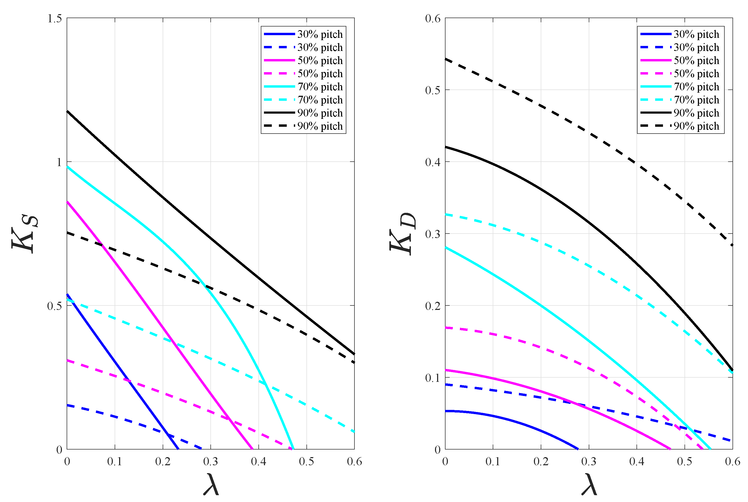
Free-running characteristics have been evaluated through a simulation campaign where and coefficients have been evaluated, in accordance with Table 1, for several and values. In particular, the evaluation of coefficients and has been performed in the pitch range from to , with steps of . Results are reported in Figure 5 that shows the comparison between propeller manufacturer data (dashed lines) and the coefficients and obtained through simulation (continuous lines). The available data concern an existing cycloidal propeller, with the same geometry of the simulated one.
The discrepancies between real and simulated data appearing in Figure 5 have been supposed to be due to the stated simplifying assumptions about the interactions among the blades. In order to overcome this issue, some correction factors have been introduced, based on physical considerations: a shielding effect that can affect the oncoming flow for some blades and the interference of each blade with the others.
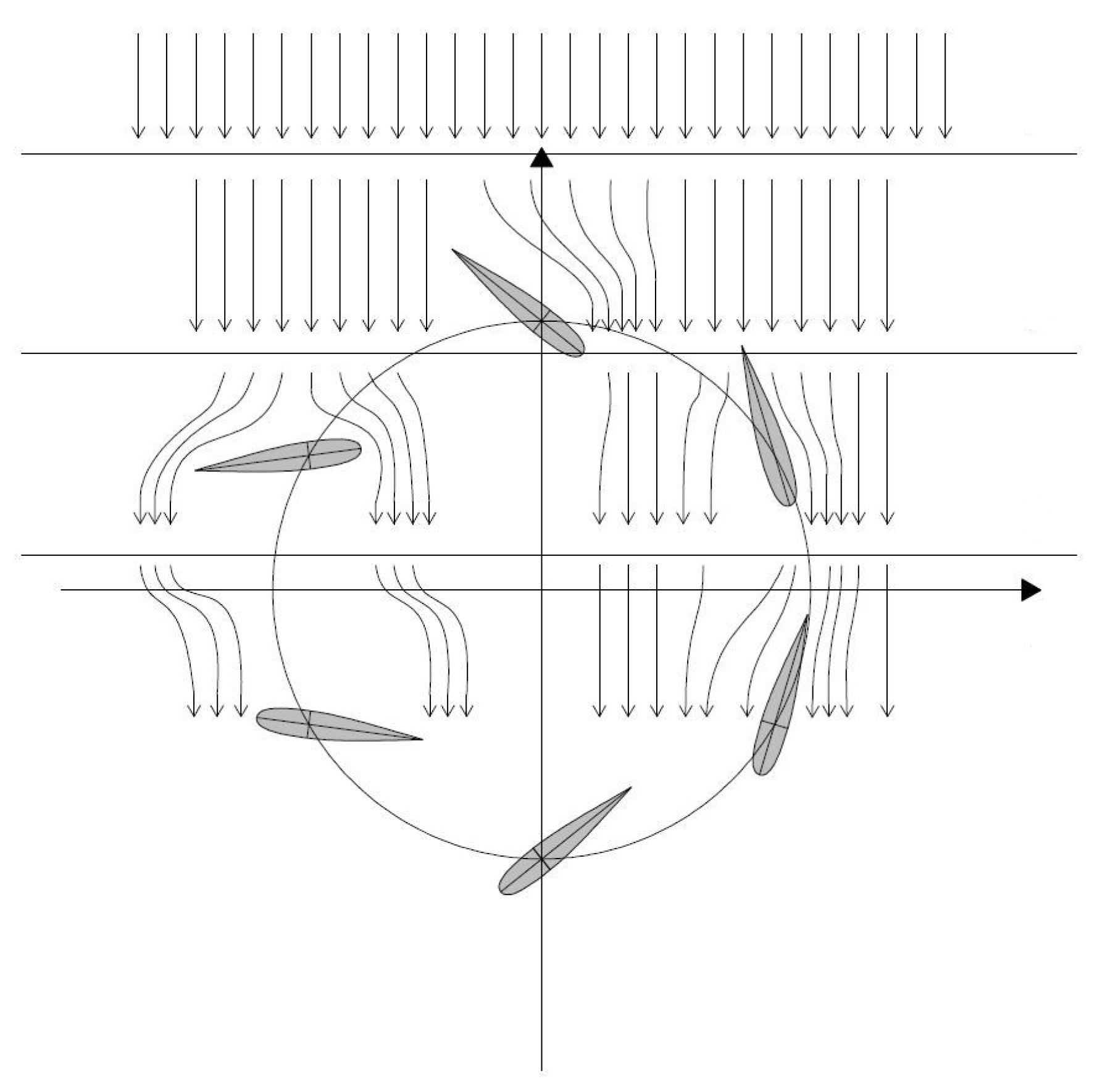
4.1. Shielding Correction
This correction concerns the shielding effect experienced by the blades that are in the half circumference not directly exposed to the oncoming water flow. Figure 6 gives a qualitative idea of how the flow is deviated by the blades. A corresponding correction factor, consisting in a matrix of corrective coefficients , has been introduced in order to reduce the velocity of the oncoming flow in the part of the rotor not directly invested by the flow itself. The corrective factors depend only on the driving pitch values and not on the advance coefficient and are implemented as it follows
where is the velocity component of the rotor center along .
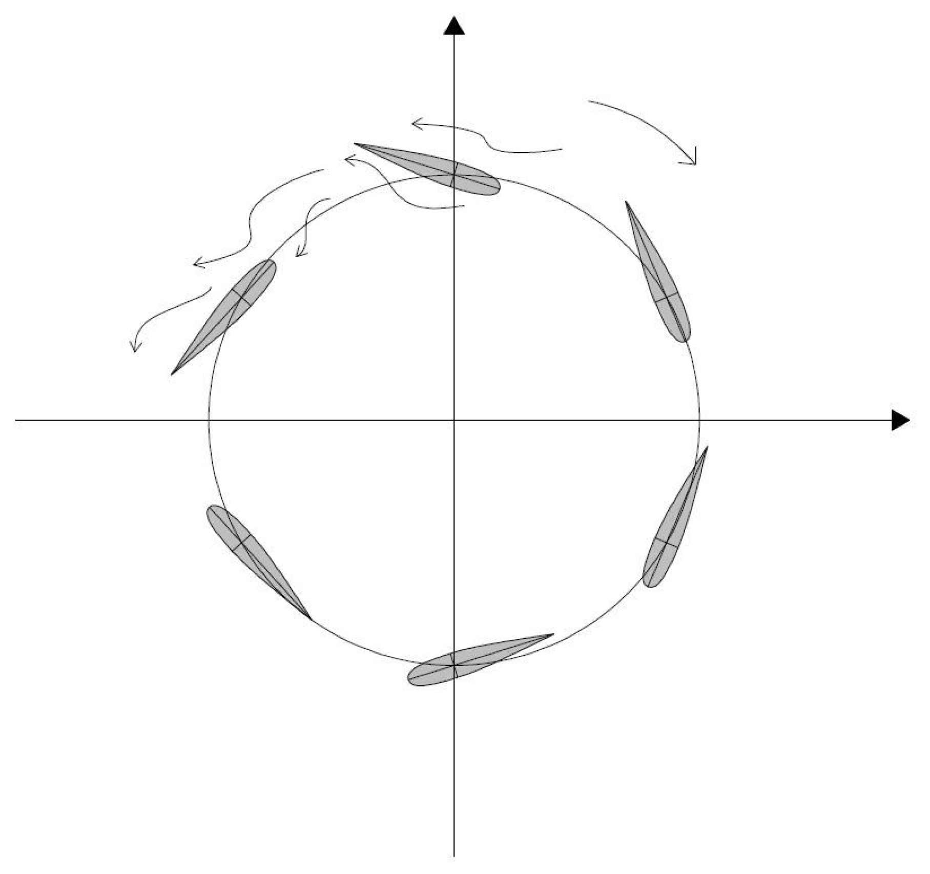
4.2. Interference Correction
As sketched in Figure 7, each blade influences the flow of the adjacent blade, so modifying the angle of attack of the incident flow itself. This interference among the blades has been modeled by reducing the attack angle of the incoming flow by a suitable quantity . This correction depends on the advance coefficient and the pitch values
where is the angle of attack defined in (15).
5. Simulation Results
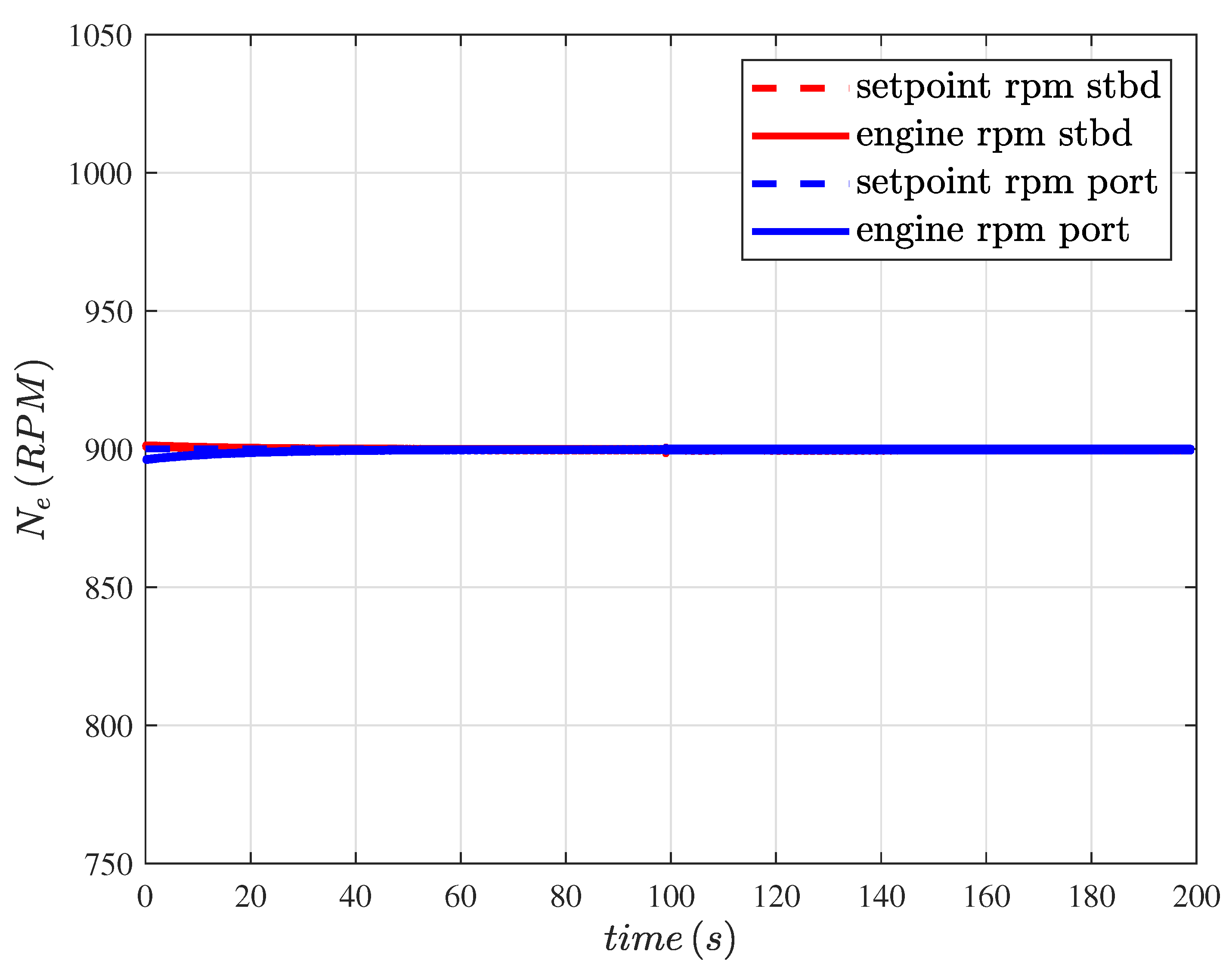
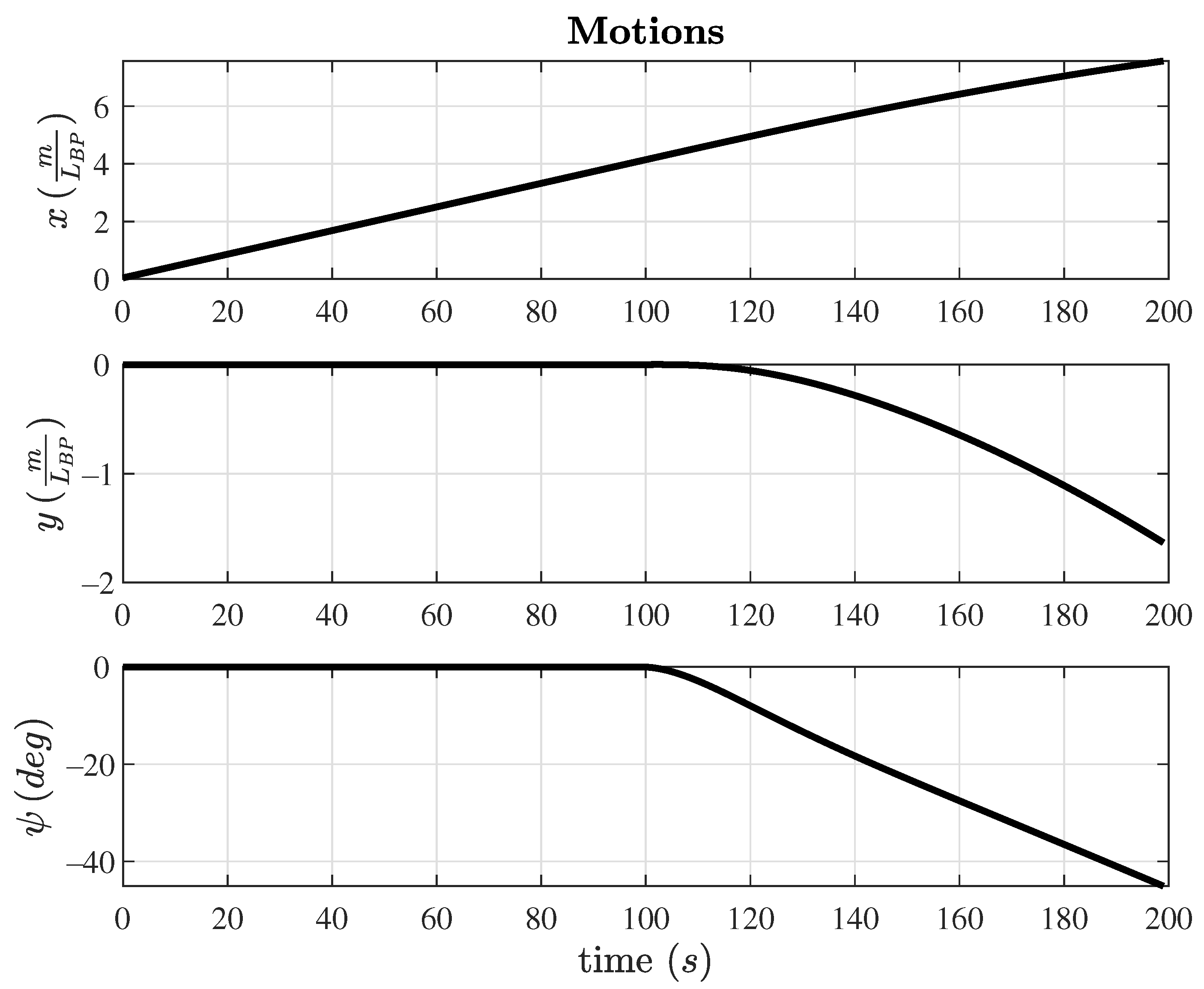
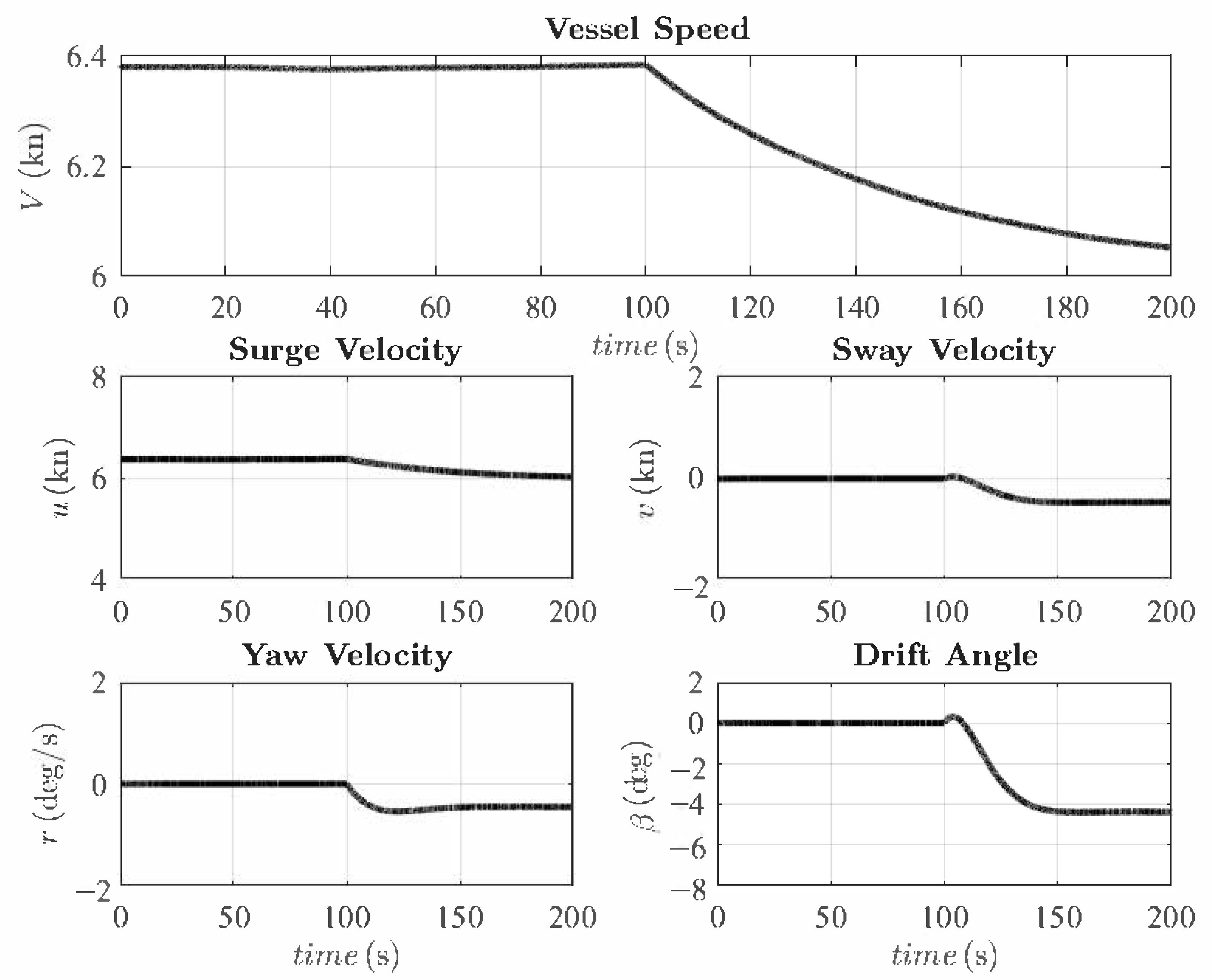
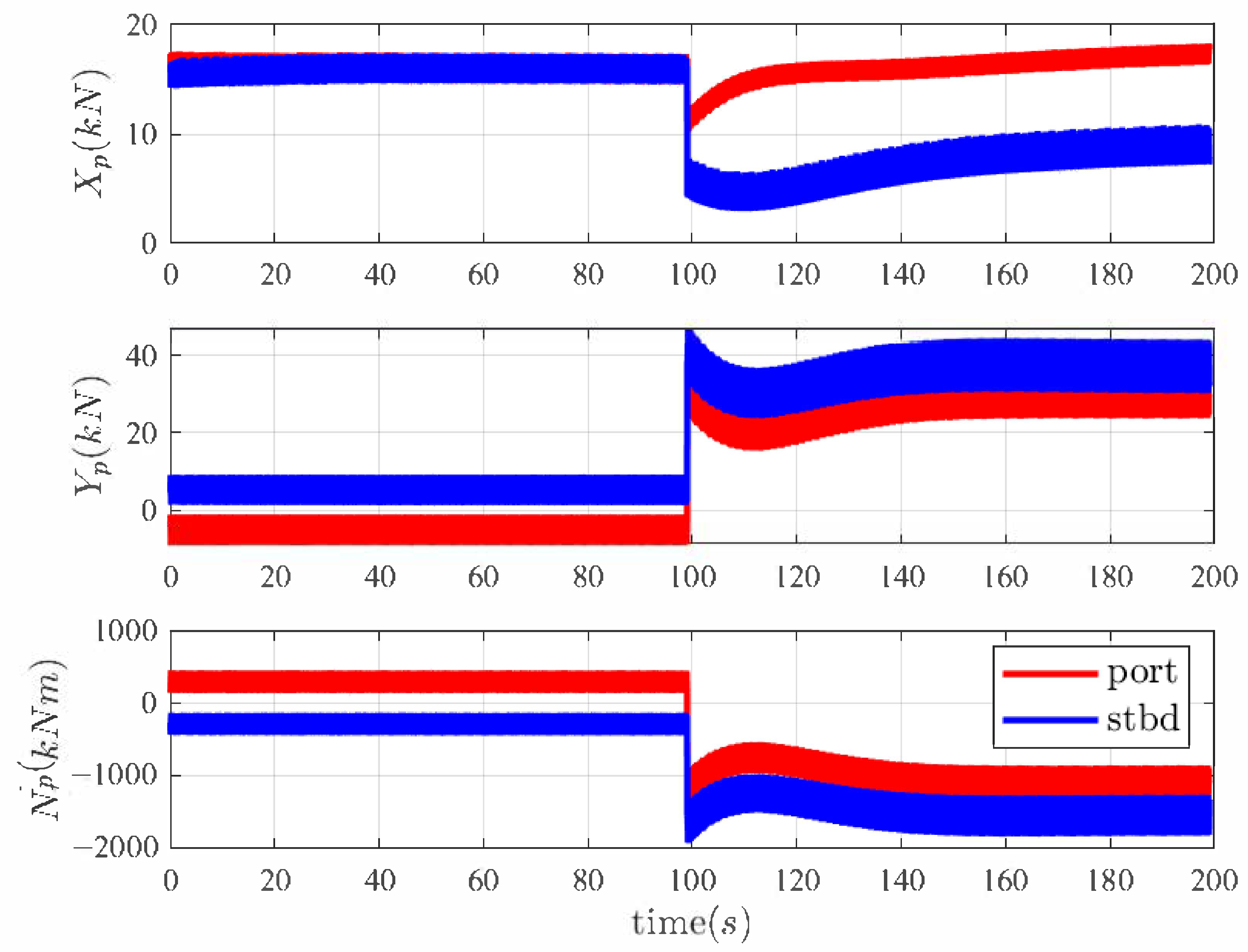
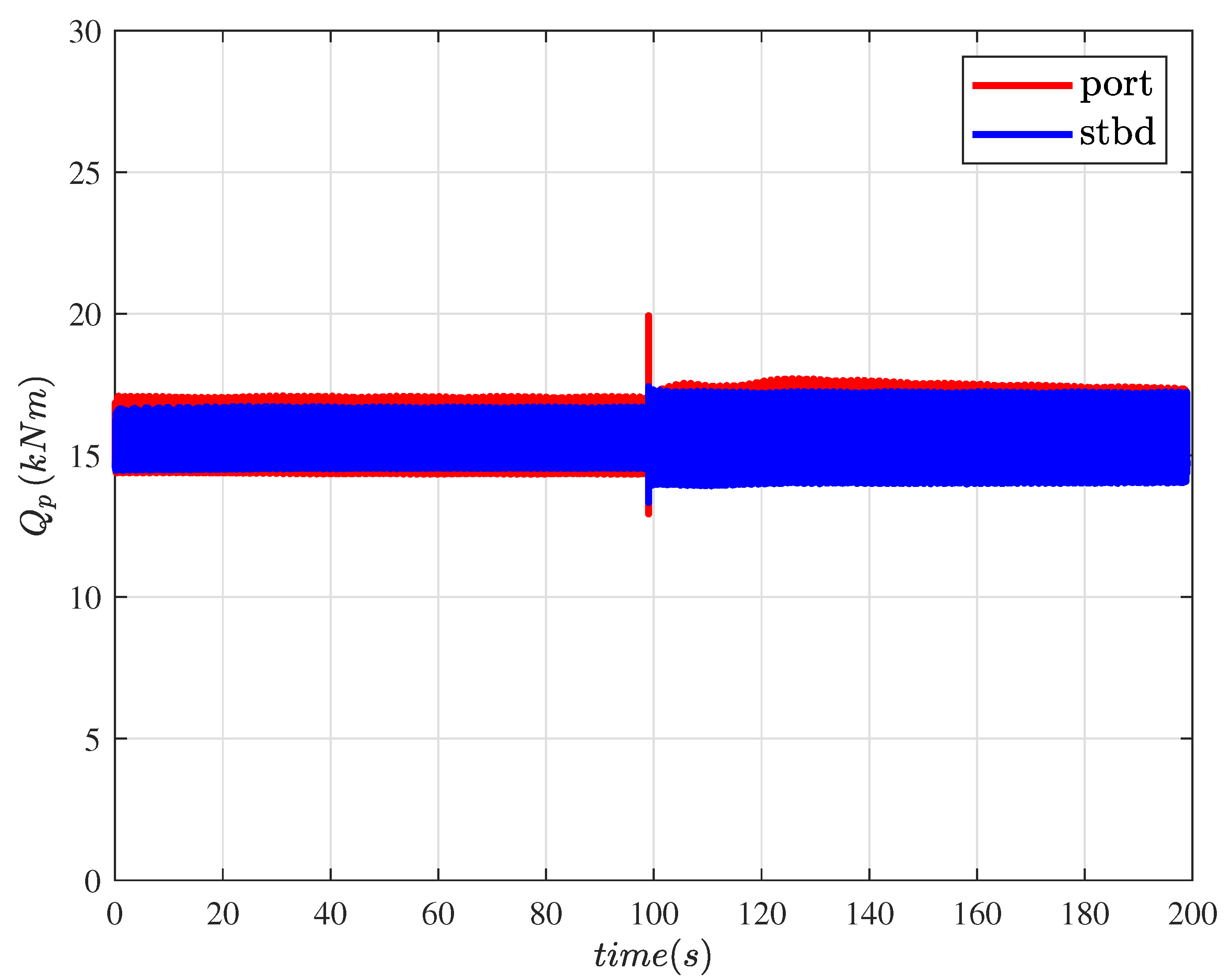
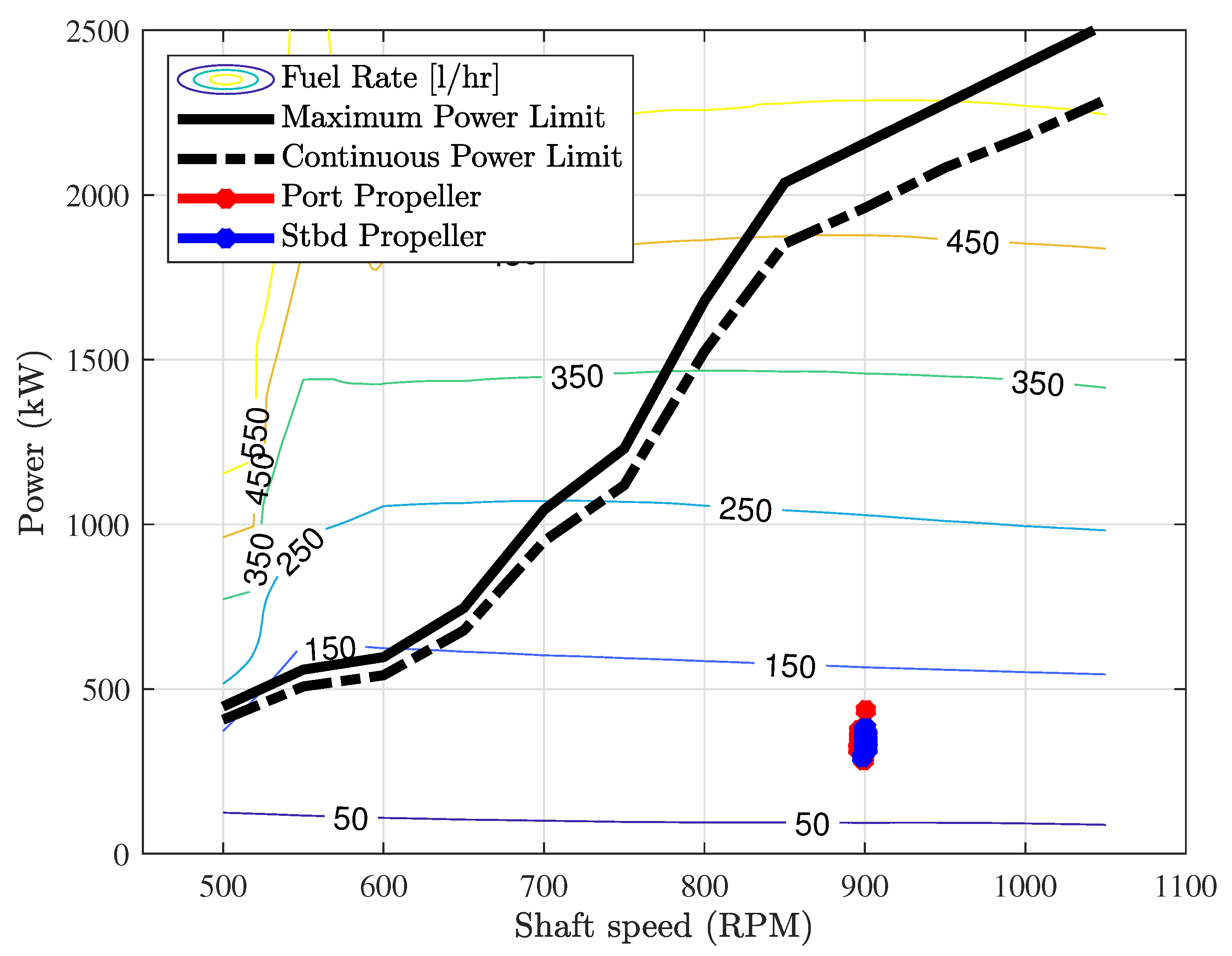
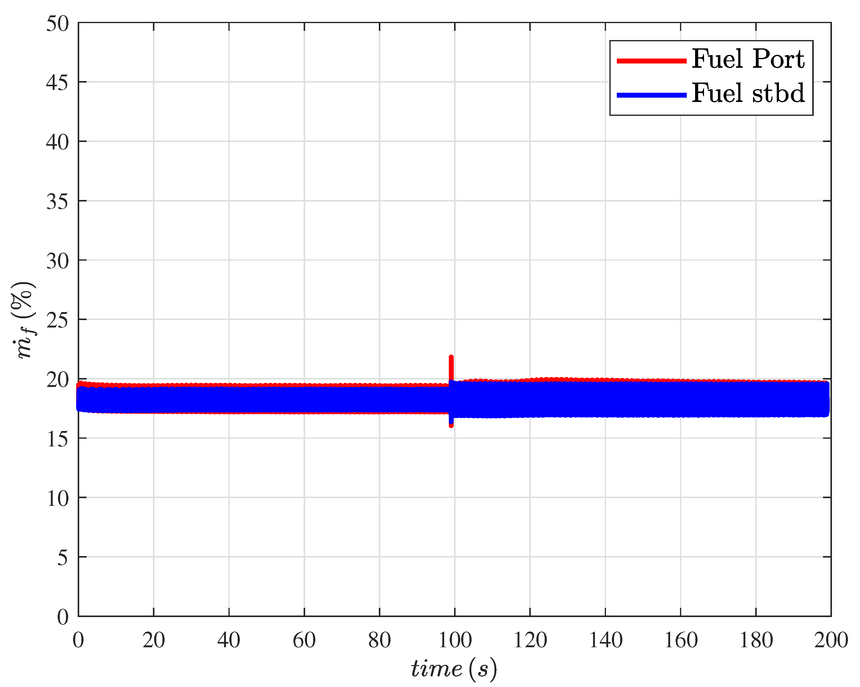
In this section results concerning a simulated maneuver are presented. In this contest, two counter rotating CPs have been fitted on a vessel, whose dynamics were known. In the proposed simulation, initially the vessel is moving forward, the propeller pitch is set at and the shaft speed is constant. At a certain instant the steering pitch is required to move from 0 to . Figure 9 shows the required and delivered shaft speed. Generally, this kind of propellers work at constant shaft speed and the thrust is controlled through the pitch value s, as for controllable pitch screw propellers. Figure 10 shows the ship motion, made dimensionless with respect to the vessel length. From top to bottom, advance motion, side drift and heading are respectively shown. Figure 11 shows the vessel speed, the components of the linear and angular vessel velocities in the body-fixed basis, and the vessel drift angle. As expected, at instant when a twenty-degree change in steeering is required and kept constant for the rest of the maneuver, the ship begins to rotate and drift, it slows down, while drift and rotation velocities increase until they stabilize to constant values. The delivered forces and moment are reported in Figure 12, where they are expressed in the basis. It is worth noticing that the model is able to evaluate the lateral forces (16) generated by each single propeller. Although two counter-rotating thrusters ensure the compensation of the lateral forces in the case of the forward navigation, this is no longer true during the maneuverings where the evaluation of such forces is an important aspect. Moreover, the implemented kinematic approach allows us to observe the asymmetry of , that is the force component along , during the evolution. This is due to the fact that the two drifting thrusters are actually undergoing two different inlet flows. Such effect is also reflected in the torque. Indeed, time histories of required torque by each propeller at the shaft are reported in Figure 13. In this case, some differences can be evaluated during the vessel rotation where load on the portside shaft is different from the starboard one. The integration of the propeller models together with the propulsion system, Figure 14, allows us to assess the matching between available power, represented by the underlying area of the black curve, and the power required by the propellers at every time–step. Portside and starboard required powers (red and blue lines respectively) are clustered in a small area of the motor load diagram. Finally, the required fuel flow rate time history is reported in Figure 15, in terms of percentage of its maximum value, allowing us to compute fuel consumption.
6. Conclusions
This work presents a simulation approach for both low and high speed manoeuvring of ships equipped with cycloidal propellers. The real strength comes from not having to calculate the propeller fluid dynamics, avoiding demanding computations that would make very difficult and complex an effective simulation of the whole ship propulsion plant behaviour (in the proposed approach, CFD method is just used for the evaluation of the lift and drag coefficients of the single blade). However, reliable results, concerning both the steady state and transient performance of the cycloidal propeller, are achieved. This is essentially due to the rigorous description of the motion of each blade and by introducing specific empirical correction factors that can be used for a preliminary performance estimation of several cycloidal propulsion units, characterized by different lengths and number of blades. In this sense, the propulsion simulator can be regarded as a parametric one. Indeed, open water diagrams can obtained for a wide range of cycloidal propellers only by changing the rotor diameter, number and length of blades. Through appropriate insights concerning the correction coefficients and therefore a dedicated hydrodynamic analysis, the simulator can reproduce the open water performance maps of other types of cycloidal thrusters, for which the literature and the industry provide very little information. Right because the lack of data, the proposed approach could be useful also to predict the behaviour of the ship during the design phase in terms of general performances, forces generation, response times and evaluation of energy/fuel consumptions. Moreover, a training platform for personnel could be implemented on this basis. Next developments should include the integration of the hydrodynamic interaction between the hull and the cycloidal propeller and vice versa, as well as the calculation of the hydrodynamic resistance of the cycloidal propellers intended as hull appendages, mainly by comparing empirical corrections with CFD results. Further improvements could include the study of different sizes of the main engine, represented by a thermodynamic model coupled to the cycloidal thruster model, in order to better analyse the engine-propeller dynamics (especially during transient conditions). Finally, the present research should be completed through a proper validation of the simulation approach, by means of experimental data of a cycloidal propulsion system installed on board a real ship.
Author Contributions
Conceptualization, M.A., S.V. and S.D.; methodology, M.A. and S.V.; software, V.S. and S.D.; validation, S.V. and S.D.; writing—original draft preparation, S.D.; writing—review and editing, M.A., S.V. and S.D. All authors have read and agreed to the published version of the manuscript.
Funding
This research received no external funding.
Institutional Review Board Statement
Not applicable.
Informed Consent Statement
Not applicable.
Data Availability Statement
Not applicable.
Conflicts of Interest
The authors declare no conflict of interest.
References
- Acanfora, M.; Montewka, J.; Hinz, T.; Matusiak, J. Towards realistic estimation of ship excessive motions in heavy weather. A case study of a containership in the Pacific Ocean. Ocean. Eng. 2017, 138, 140–150. [Google Scholar] [CrossRef]
- Acanfora, M.; Altosole, M.; Balsamo, F.; Micoli, L.; Campora, U. Simulation Modeling of a Ship Propulsion System in Waves for Control Purposes. J. Mar. Sci. Eng. 2022, 10, 36. [Google Scholar] [CrossRef]
- Altosole, M.; Boote, D.; Brizzolara, S.; Viviani, M. Integration of Numerical Modeling and Simulation Techniques for the Analysis of Towing Operations of Cargo Ships. Int. Rev. Mech. Eng. 2013, 7, 1236–1245. [Google Scholar]
- Altosole, M.; Figari, M.; Martelli, M.; Orrù, G. Propulsion control optimisation for emergency manoeuvres of naval vessels. In Proceedings of the INEC 2012-11th International Naval Engineering Conference and Exhibition, Edinburgh, UK, 15–17 May 2012. [Google Scholar]
- Ghaemi, M.; Zeraatgar, H. Analysis of hull, propeller and engine interactions in regular waves by a combination of experiment and simulation. J. Mar. Sci. Technol. 2021, 26, 257–272. [Google Scholar] [CrossRef]
- Saettone, S.; Tavakoli, S.; Taskar, B.; Jensen, M.V.; Pedersen, E.; Schramm, J.; Steen, S.; Andersen, P. The importance of the engine-propeller model accuracy on the performance prediction of a marine propulsion system in the presence of waves. Appl. Ocean. Res. 2020, 103, 102320. [Google Scholar] [CrossRef]
- Altosole, M.; Campora, U.; Martelli, M.; Figari, M. Performance decay analysis of a marine gas turbine propulsion system. J. Ship Res. 2014, 58, 117–129. [Google Scholar] [CrossRef]
- Zaccone, R.; Altosole, M.; Figari, M.; Campora, U. Diesel engine and propulsion diagnostics of a mini-cruise ship by using artificial neural networks. In Proceedings of the 16th International Congress of the International Maritime Association of the Mediterranean, Pula, Croatia, 21–24 September 2015; pp. 593–602. [Google Scholar] [CrossRef]
- Campora, U.; Capelli, M.; Cravero, C.; Zaccone, R. Metamodels of a gas turbine powered marine propulsion system for simulation and diagnostic purposes. J. Nav. Archit. Mar. Eng. 2015, 12, 1–14. [Google Scholar] [CrossRef] [Green Version]
- Halder, A.; Walther, C.; Benedict, M. Hydrodynamic modeling and experimental validation of a cycloidal propeller. Ocean. Eng. 2018, 154, 94–105. [Google Scholar] [CrossRef]
- Hu, J.; Li, T.; Guo, C. Two-dimensional simulation of the hydrodynamic performance of a cycloidal propeller. Ocean. Eng. 2020, 217, 107819. [Google Scholar] [CrossRef]
- Prabhu, J.; Nagarajan, V.; Sunny, M.; Sha, O. On the fluid structure interaction of a marine cycloidal propeller. Appl. Ocean. Res. 2017, 64, 105–127. [Google Scholar] [CrossRef]
- Bakhtiari, M.; Ghassemi, H. CFD data based neural network functions for predicting hydrodynamic performance of a low-pitch marine cycloidal propeller. Appl. Ocean. Res. 2020, 94, 101981. [Google Scholar] [CrossRef]
- Prabhu, J.; Dash, A.; Nagarajan, V.; Sha, O. On the hydrodynamic loading of marine cycloidal propeller during maneuvering. Appl. Ocean. Res. 2019, 86, 87–110. [Google Scholar] [CrossRef]
- Altosole, M.; Donnarumma, S.; Spagnolo, V.; Vignolo, S. Marine cycloidal propulsion modelling for DP applications. In Proceedings of the VI International Conference on Computational Methods in Marine Engineering, Rome, Italy, 15–17 June 2017; pp. 206–219. [Google Scholar]
- Altosole, M.; Donnarumma, S.; Spagnolo, V.; Vignolo, S. Simulation of a marine dynamic positioning system equipped with cycloidal propellers. In Progress in Maritime Technology and Engineering; CRC Press/Balkema: Boca Raton, FL, USA, 2018; pp. 257–264. [Google Scholar]
- Donnarumma, S.; Figari, M.; Martelli, M.; Vignolo, S.; Viviani, M. Design and Validation of Dynamic Positioning for Marine Systems: A Case Study. IEEE J. Ocean. Eng. 2018, 43, 677–688. [Google Scholar] [CrossRef] [Green Version]
- Donnarumma, S.; Figari, M.; Martelli, M.; Zaccone, R. Simulation of the Guidance and Control Systems for Underactuated Vessels. In Proceedings of the International Conference on Modelling and Simulation for Autonomous Systems, Palermo, Italy, 29–31 October 2019; Springer: Cham, Switzerland, 2020; Volume 11995, pp. 108–119. [Google Scholar] [CrossRef]
- Martelli, M.; Viviani, M.; Altosole, M.; Figari, M.; Vignolo, S. Numerical modelling of propulsion, control and ship motions in 6 degrees of freedom. Proc. Inst. Mech. Eng. 2014, 228, 373–397. [Google Scholar] [CrossRef]
- Martelli, M.; Figari, M.; Altosole, M.; Vignolo, S. Controllable pitch propeller actuating mechanism, modelling and simulation. Proc. Inst. Mech. Eng. Part J. Eng. Marit. Environ. 2014, 228, 29–43. [Google Scholar] [CrossRef]
- Battistoni, L. Numerical Simulation Approach for the Preliminary Design of a Cycloidal Propeller. Master’s Thesis, University of Genoa, Genoa, Italy, 2014. [Google Scholar]
Figure 1.
Vessel model layout.

Figure 2.
General overview of voith installation on a vessel on the top and some sketch of the machinery.
Figure 2.
General overview of voith installation on a vessel on the top and some sketch of the machinery.

Figure 3.
Kinematics of the blade.

Figure 4.
Layout of propulsion simulation platform.

Figure 5.
Thrust and torque propeller coefficients: model (solid lines) VS manufacturer data (dashed lines).
Figure 5.
Thrust and torque propeller coefficients: model (solid lines) VS manufacturer data (dashed lines).

Figure 6.
Shielding phenomena [21].
Figure 6.
Shielding phenomena [21].

Figure 7.
Interference phenomena [21].
Figure 7.
Interference phenomena [21].

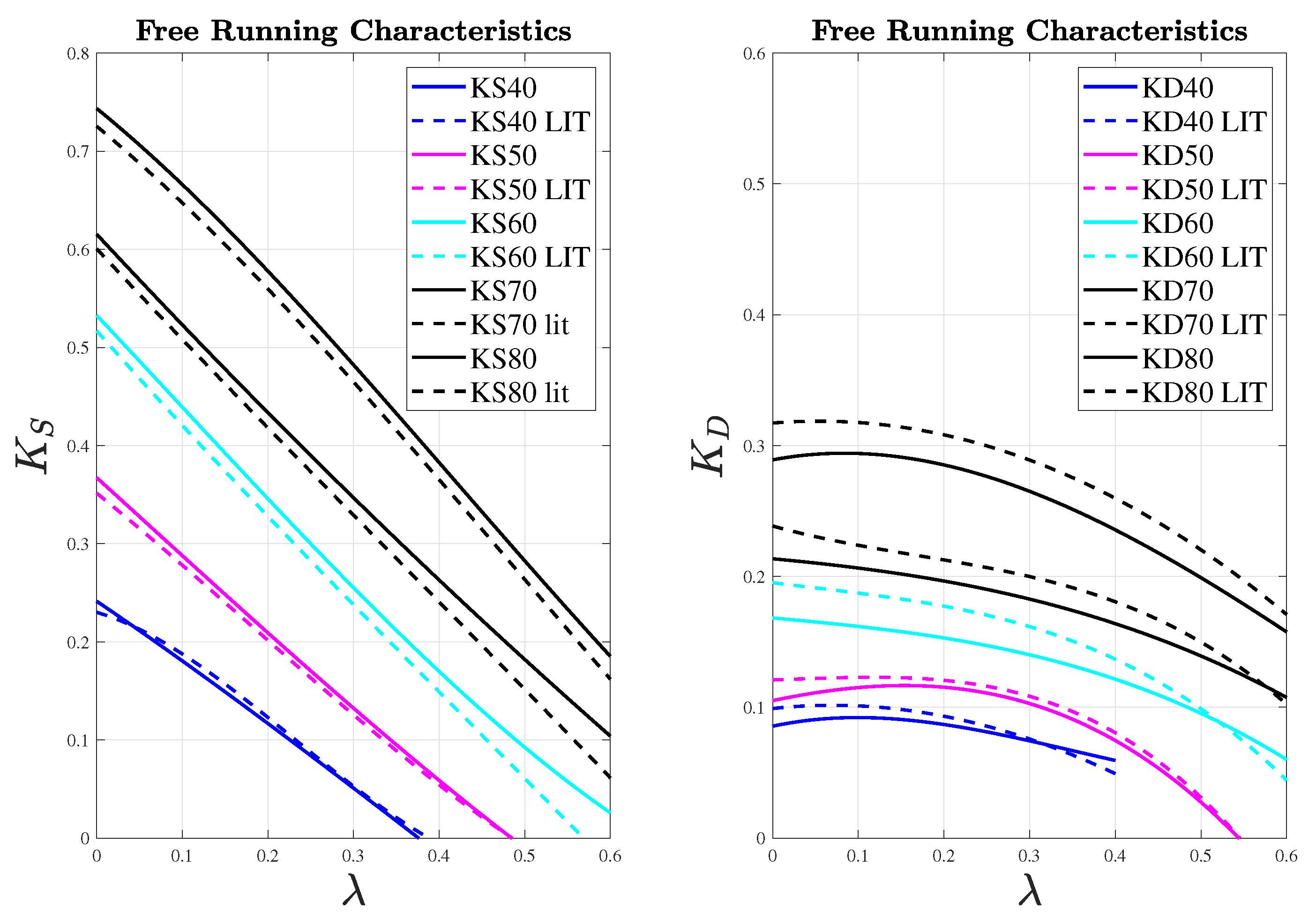
Figure 8.
Thrust and torque propeller coefficients: model (solid lines) VS manufacturer (dashed lines) data.
Figure 8.
Thrust and torque propeller coefficients: model (solid lines) VS manufacturer (dashed lines) data.

Figure 9.
Engine shaft speed setpoint and feedback.

Figure 10.
Vessel motions.

Figure 11.
Vessel speed and velocity components in the body-fixed basis.

Figure 12.
Propeller delivered forces and moment.

Figure 13.
Propeller torque.

Figure 14.
Propeller required power on the engine load diagram.

Figure 15.
Fuel flow time history.


Table 1.
Cycloidal and screw propeller non-dimensional coefficients.
| Coefficients | Cycloidal | Screw |
|---|---|---|
| advance coefficient | ||
| thrust coefficient | ||
| torque coefficient | ||
| efficiency |
where
is the advance velocity, T is the propeller thrust, M and are the CP and screw propeller torque
respectively, L is the blade length, D is the rotor diameter, is the sea water density, L is the blade length, u is
the tangential speed (u = nπD).
Table 2.
Geometric parameters of the propeller.
| Parameter | Value |
|---|---|
| Number of blades | 5 |
Publisher’s Note: MDPI stays neutral with regard to jurisdictional claims in published maps and institutional affiliations. |
© 2022 by the authors. Licensee MDPI, Basel, Switzerland. This article is an open access article distributed under the terms and conditions of the Creative Commons Attribution (CC BY) license (https://creativecommons.org/licenses/by/4.0/).
Share and Cite
MDPI and ACS Style
Altosole, M.; Donnarumma, S.; Spagnolo, V.; Vignolo, S. Performance Simulation of Marine Cycloidal Propellers: A Both Theoretical and Heuristic Approach. J. Mar. Sci. Eng. 2022, 10, 505. https://doi.org/10.3390/jmse10040505
AMA Style
Altosole M, Donnarumma S, Spagnolo V, Vignolo S. Performance Simulation of Marine Cycloidal Propellers: A Both Theoretical and Heuristic Approach. Journal of Marine Science and Engineering. 2022; 10(4):505. https://doi.org/10.3390/jmse10040505
Chicago/Turabian StyleAltosole, Marco, Silvia Donnarumma, Valentina Spagnolo, and Stefano Vignolo. 2022. "Performance Simulation of Marine Cycloidal Propellers: A Both Theoretical and Heuristic Approach" Journal of Marine Science and Engineering 10, no. 4: 505. https://doi.org/10.3390/jmse10040505
Note that from the first issue of 2016, this journal uses article numbers instead of page numbers. See further details here.