Machining Chatter Prediction Using a Data Learning Model

Abstract

Machining processes, including turning, are a critical capability for discrete part production. One limitation to high material removal rates and reduced cost in these processes is chatter, or unstable spindle speed-chip width combinations that exhibit a self-excited vibration. In this paper, an artificial neural network (ANN)—a data learning model—is applied to model turning stability. The novel approach is to use a physics-based process model—the analytical stability limit—to generate a (synthetic) data set that trains the ANN. This enables the process physics to be combined with data learning in a hybrid approach. As anticipated, it is observed that the number and distribution of training points influences the ability of the ANN model to capture the smaller, more closely spaced lobes that occur at lower spindle speeds. Overall, the ANN is successful (>90% accuracy) at predicting the stability behavior after appropriate training.

1. Introduction

Material removal processes, including turning and milling, are widely applied in industry. While significant advances have been achieved over the last decades, one limitation to high material removal rates is chatter, or unstable cutting conditions. The result is poor surface quality and potential damage to the tool, workpiece, and machine.

The control of stability in turning operations is crucial in industry and ongoing research efforts address chatter avoidance. Siddhpura and Paurobally [1] completed a literature review of chatter prediction in turning. They classified the techniques for chatter stability prediction as stability lobe diagrams, Nyquist plots, and finite element analyses. Their study also discussed the experimental techniques for chatter stability prediction and detection and separated them into three main groups: signal acquisition and processing techniques; chip analysis; and artificial intelligence techniques, including neural networks, hidden Markov models, and fuzzy logic. The authors noted that the number of publications featuring artificial intelligence techniques was low at the time of publication (only 11 from 1978 to 2012), although additional work has been done since then.

Chanda and Dwivedy [2] developed the governing nonlinear equations of motion for turning, considering both the workpiece and the tool to be flexible. The regenerative effect due to inherent time delay was considered. Copenhaver et al. [3] described a periodic sampling-based method for identifying the stability of modulated tool path turning (MTP). They compared a periodic sampling metric with the traditional frequency domain approach, where the frequency spectrum is analyzed to identify the turning stability.

Filippov et al. [4] studied the transition from the stable turning to chatter using acoustic emission signals. High frequency peaks appeared in transition to the chatter mode. A mathematical model of turning was presented by Gerasimenko et al. [5], where the stability limit for turning a thin-walled cylindrical part was defined. Gouskova et al. [6] determined the stability of a continuous cutting process for an arbitrary arrangement of two cutters. Gyebroszki et al. [7] created two models and combined them later, a surface regeneration model for turning operations and a chip formation model. They compared the results obtained and found that the time scale for the second model (chip formation) was smaller than the first one.

Hajdu et al. [8] incorporated noise and uncertainties in chatter predictions. In their approach, they did not apply filtering or parameter identification to the frequency response functions (FRFs) and presented a frequency domain method for the analysis of stability in machining. In the application of this method to a model for orthogonal cutting, the authors found that the robust stability boundaries are lower to those showed by the FRF alone. Huang et al. [9] also considered uncertainties in their analysis. They used a probabilistic method (Monte Carlo simulation) and found that, when compared with a deterministic solution, Monte Carlo simulation provided better results by considering the influence of random parameters.

Mousavi et al. [10] presented a numerical approach for the prediction of a manipulator behavior in machining tasks. They established theoretical stability limits taking into account the variability of the robot dynamics within its workspace. This made an auto-adaptation of cutting parameters and robot configurations along the trajectory possible. The authors generated a stability diagram for chatter in milling taking into account the kinematic redundancy variable. The theory was validated with experimental robotic machining trials. Liu et al. [11] investigated the probability of stability for turning. The authors defined and represented a reliability lobe diagram to identify stable and unstable zones, rather than the traditional stability lobe diagram (SLD). The reliability was calculated using the FOSM (first-order second moment) and Monte Carlo methods, and was compared to the traditional stability lobe diagram.

Khasawneh and Munch [12] proposed a new approach for determining the stability of stochastic dynamical systems by examining their time series using topological data analysis. Two statistical approaches (three sigma edit rule analysis and principal component analysis) were used by Jiménez et al. [13] to predict chatter, obtaining accuracy rates over 75%.

The receptance coupling method was used by Jasiewicz and Powalka [14] for determining the lathe workpiece dynamics and inverse receptance coupling was applied for the spindle dynamics. Lu et al. [15] focused on turning process and proposed a model for chatter prediction for turning a tailstock-supported flexible rod. They considered the tool position effect along the workpiece axis. The variation of theoretical and experimental tool locations was within 9%.

Tyler et al. [16] studied the process damping force in turning to propose a stability model. This was dependent on several variables, including the chip width and cutting speed. Experiments were completed to validate the time domain simulation, which provided accurate predictions.

Chatter prediction using machine learning techniques has also been studied, including neural networks, support vector machines, and others. Ahmad et al. [17] developed two different models of extreme learning techniques using random weights and hidden nodes. Lamraoui et al. [18] applied a neural network (NN) and the input data based on signal analysis was used to predict milling stability. Gupta et al. [19] based their research on the combination of several artificial techniques, such as support vector regression (SVR), genetic algorithms (GA) or artificial neural networks (ANN). They trained the model using the process parameters as input values. Power, tool wear and surface roughness were the output variables.

Jurkovic et al. [20] compared the performance of three machine learning methods for the prediction of operating parameters in high-speed turning. Observed parameters were the surface roughness (Ra), cutting force (F_c), and tool life (T). Polynomial (quadratic) regression, SVR, and ANN were used. Polynomial regression demonstrated the best performance in for F_c and Ra prediction, while the ANN showed the best performance for T prediction.

Khasawneh et al. [21] combined several deterministic and stochastic models to create persistence diagrams of turning stability. The approach was intended for chatter classification using signals produced by complicated and noisy manufacturing systems. Yao et al. [22] developed a vector for chatter prediction in machining. It was based on the wavelet packet energy ratio in the frequency band and the standard deviation of the wavelet transform. This vector was then used to generate a support vector machine (SVM) for pattern recognition, which was classified in three categories: stable, transition, and chatter. Zagorski et al. [23] employed two NNs for chatter detection in milling: radial basis function (RBF) and multi-layered perceptron (MLP). Kumar and Singh [24] used an ANN based on feed forward backpropagation to predict stability in turning, also focusing on the metal removing index. The authors applied a tangent sigmoid activation function for model training.

In this paper, an ANN is used to model stability behavior in turning, where the physics-based analytical stability limit is applied to generate a data set that trains the ANN. The motivation for this effort is that the ANN model inputs are the spindle speed and depth of cut, while the analytical stability limit model inputs are the structural dynamics and force model. When experimental stability data is collected at a selected spindle speed depth of cut pair, a model which can accept this data directly is preferred. The ANN enables this convenient model updating.

2. Background

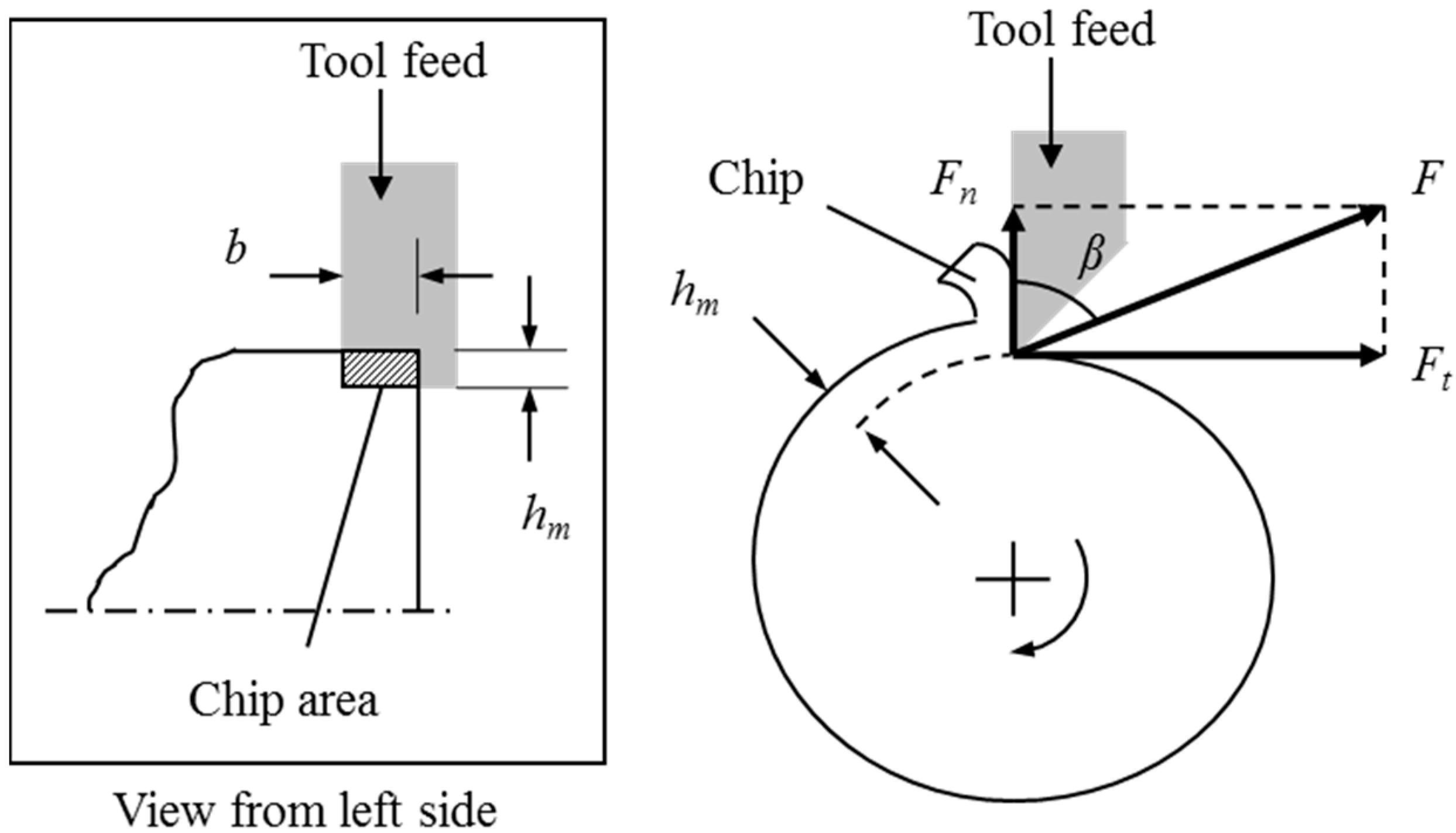
During turning, a sharp cutting edge is used to remove material in the form of a chip. Figure 1 shows an orthogonal cutting operation, where only the normal, F_n, and tangential, F_t, components of the resultant force, F, are considered [25]. In general, the cutting force vector includes the third component along the workpiece rotation axis, but the orthogonal (planar) treatment is sufficient to describe the process dynamics. The figure also identifies: (1) The mean chip thickness, h_m, or commanded feed per revolution for the facing operation pictured, and (2) the force angle, β, between F and F_n. The side view of this operation (inset in Figure 1) identifies the chip width, b. Together, the chip thickness and chip width define the area of material to be removed, A = bh_m.

The cutting force can be approximated as the product of the chip area and the process dependent specific (per unit area) force coefficient, K_s [26]. It depends on the workpiece material, tool geometry, and, to a lesser extent, the cutting speed (peripheral velocity of the rotating workpiece) and chip thickness.

$$F=K_{s}A=K_{s}b{h}_m$$

(1)

The normal and tangential components, F_n and F_t, can be expressed using F and the force angle:

$$F_n=\cos \beta F=\cos \beta K_{s}b{h}_m=k_{n}b{h}_m$$

(2)

and

$$F_t=\sin \beta F=\sin \beta K_{s}b{h}_m=k_{t}b{h}_m,$$

(3)

where the cutting force coefficients, k_n and k_t, are introduced which incorporate both K_s and β. A common approach used to characterize these process dependent values is to prescribe known cutting conditions and measure the force components directly [26]. As an alternative, the material behavior can be defined using a constitutive model (e.g., Johnson–Cook) and the cutting force predicted using finite element simulations.

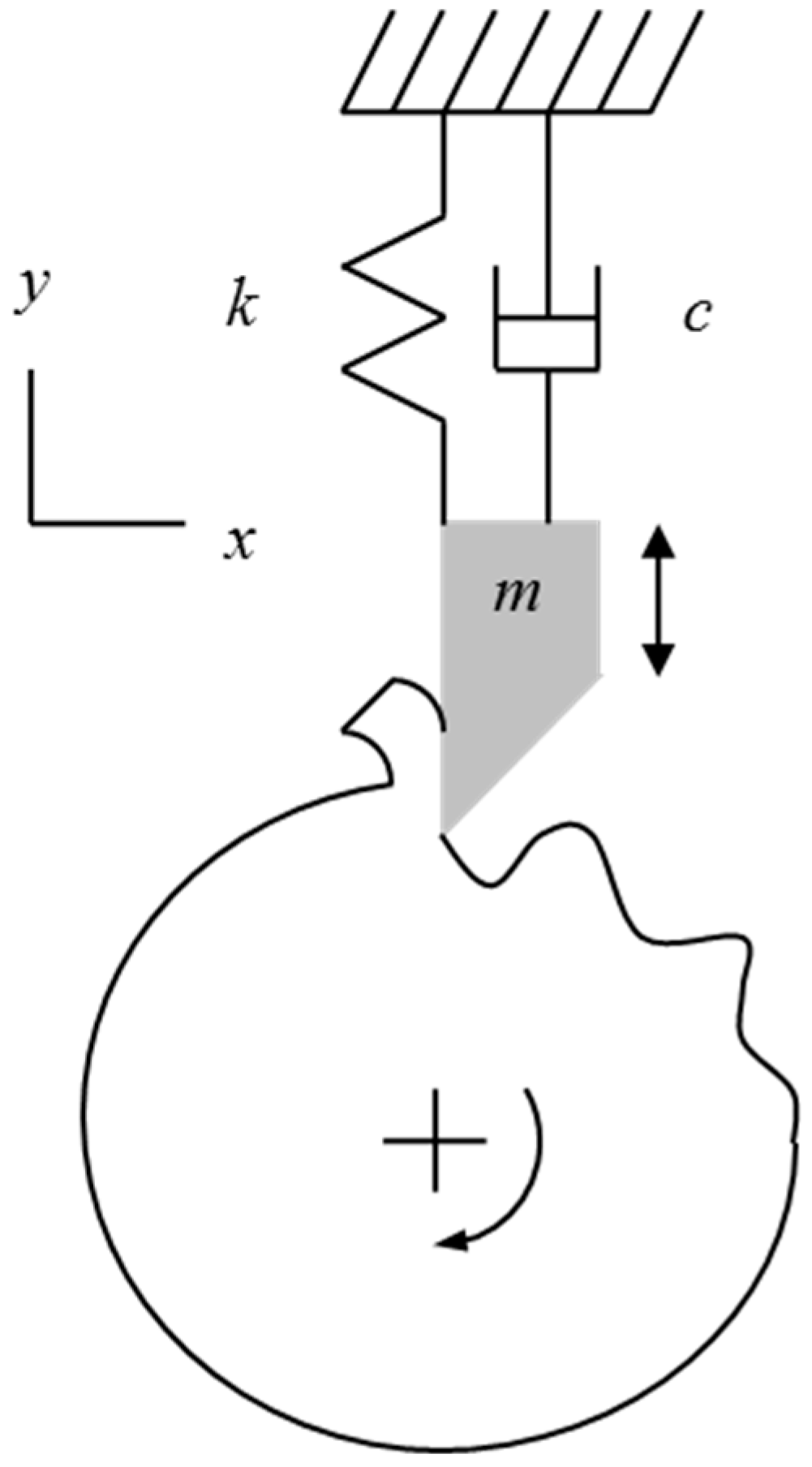
The cutting force causes deflections of the cutting tool. Because the tool has stiffness and mass, it can vibrate. If the tool is vibrating as it removes material, these vibrations are imprinted on the workpiece surface as a wavy profile. Figure 2 shows an exaggerated view, where the initial impact with the workpiece surface causes the tool to begin vibrating, and the oscillations in the normal direction to be copied onto the workpiece. When the workpiece begins its second revolution, the vibrating tool encounters the wavy surface produced during the first revolution. Therefore, the chip thickness at any instant depends both on the tool deflection at that time and the workpiece surface from the previous revolution(s). Vibration of the tool therefore leads to a variable chip thickness which, according to Equation (1), yields a variable cutting force since the force is proportional to the chip thickness. The cutting force governs the current tool deflection and, subsequently, the system exhibits feedback.

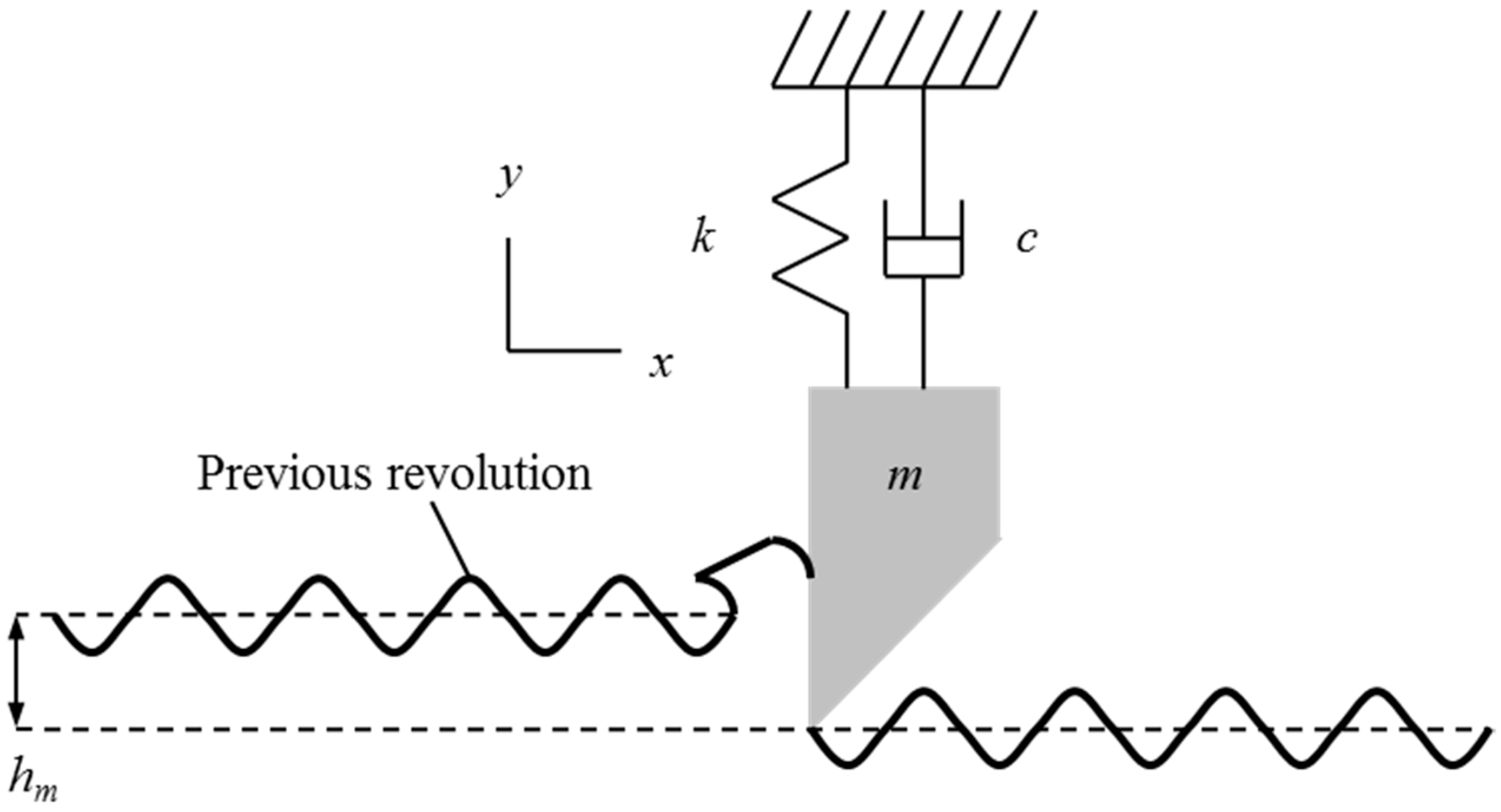
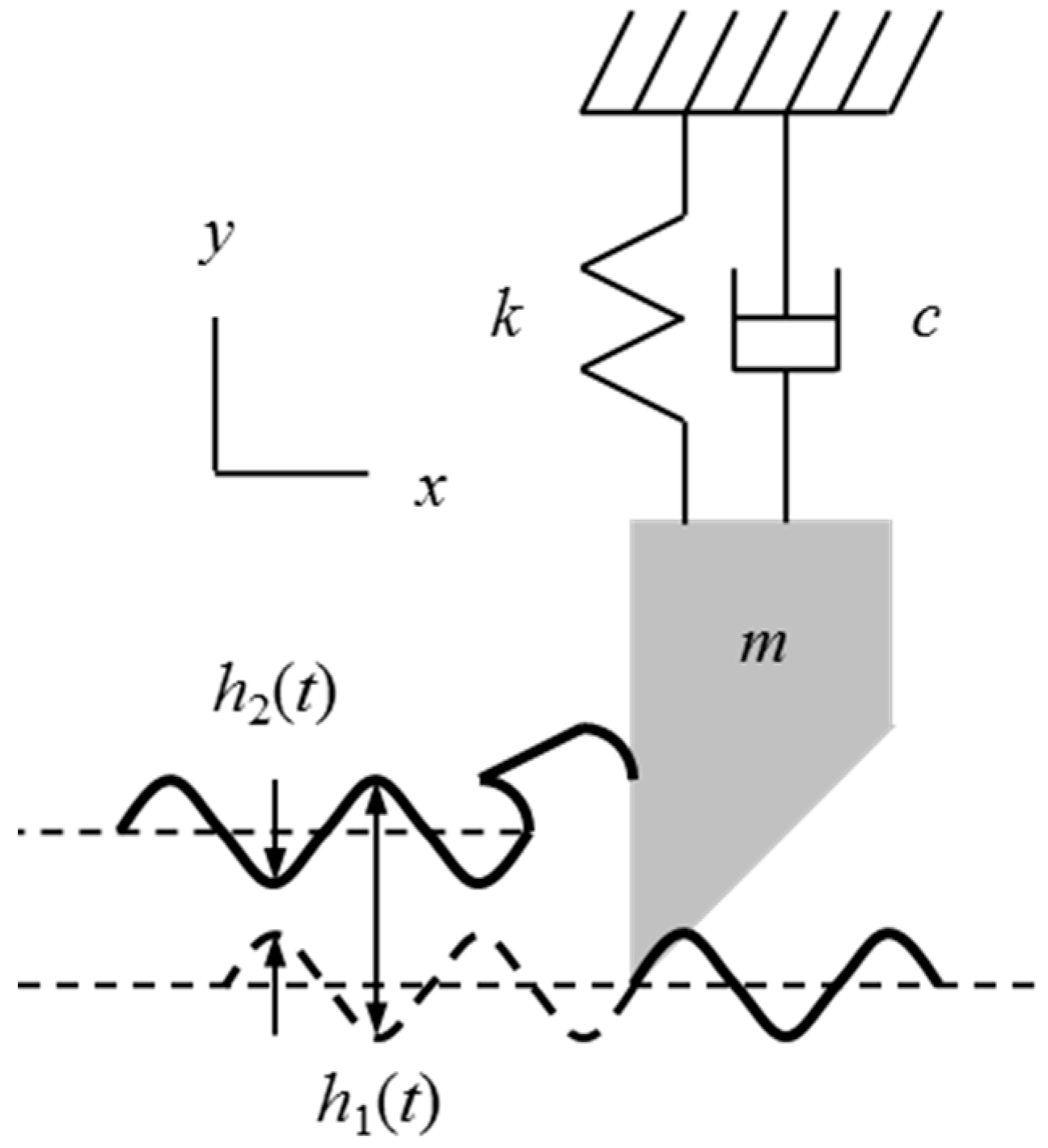
From a modeling standpoint, this “regeneration of waviness” appears as a time-delayed term in the chip thickness equation. Figure 3 shows an unwrapped view of the turning operation, where the surface on the left was produced in the previous revolution and the surface to the right of the tool (offset by the mean feed per revolution) was just cut away by the oscillating tool. Only the vibrations in the normal direction, y (positive direction out of the cut), are considered here because they have the most direct influence on the chip thickness.

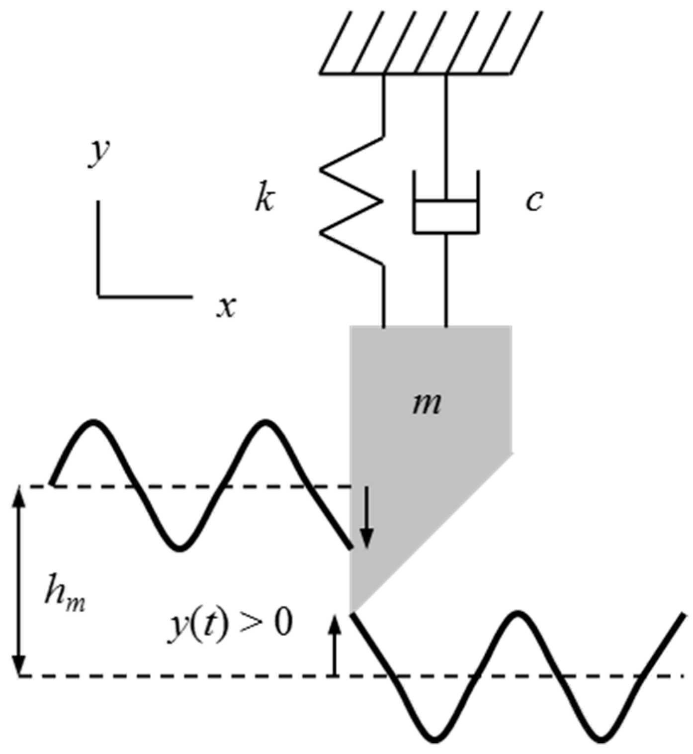
The time dependent, instantaneous chip thickness, h(t), is determined using Equation (4). It is seen that a larger positive vibration during the previous revolution, y(t − τ), where τ is the time for one rotation, gives an increased chip thickness (i.e., less material was removed so the current chip is thicker). A larger positive current vibration, y(t), on the other hand, yields a thinner chip, see Figure 4.

$$h\left(t\right)=h_m+y\left(t-\tau \right)-y\left(t\right)$$

(4)

The relative phasing between the surface waviness from one pass to the next determines the level of force variation and whether the operation is stable or unstable (chatter occurs). Figure 5 and Figure 6 show two possibilities. In Figure 5, the wavy surfaces between two revolutions are in phase. Therefore, even though vibration is present during material removal, the chip thickness variation (vertical distance between the two curves) is negligible and there is no appreciable force variation. This enables stable cutting at larger chip widths. Considering that the tool tends to vibrate at its natural frequency, it is intuitive that matching the workpiece rotating frequency (spindle speed) to the tool’s natural frequency will lead to this preferred “in phase” situation. However, this is counter-intuitive based on a traditional understanding of resonance, where driving the system at its natural frequency is typically avoided because the vibration amplitude is large. While it is understood that the vibration magnitude is larger, it has been demonstrated through both theory and experiment that increased material removal rate is beneficial. In milling, a phenomenon referred to as surface location error (SLE) has been studied, where the final location of the machined surface depends on the location of the tool in its vibration cycle when it is leaving the surface. It has been shown that SLE is large at resonance and sensitive to changes in the system dynamics (e.g., natural frequency) [25]. Figure 6 shows a less favorable phase relationship where there is significant variation in the chip thickness. This leads to unstable cutting at smaller chip widths than the previous case due to the force variations and subsequent tool deflections.

Depending on the feedback system “gain”, or chip width b, and spindle speed, Ω, the turning operation will either be stable or exhibit chatter, which causes large vibrations and forces and leads to poor surface finish and, potentially, tool/workpiece damage. In stable machining, the vibrations diminish from revolution to revolution. In unstable machining, the vibrations grow from revolution to revolution until limited in some way. Surprisingly, the vibrations may become large enough that the tool jumps out of the cut, losing contact with the workpiece. The vibrations in unstable cutting may be at least as large as the chip thickness and it is not surprising that these large vibrations may result in damage to the machine, tool, and workpiece. The governing relationships for this behavior are provided in Equations (5)–(7) [25]. In these equations, b_lim is the limiting chip width to avoid chatter, f_c is the chatter frequency (should it occur), FRF is the frequency response function that describes the tool’s dynamic response, N is the integer number of waves of vibration imprinted on the workpiece surface in one revolution, and $\frac{\epsilon }{2\pi }$ is any additional fraction of a wave, where ε is the phase (in rad) between current and previous tool vibrations.

$$b_{lim}=\frac{-1}{2K_s\cos \beta Re\left[FRF\right]}$$

(5)

$$\frac{f_c}{\Omega }=N+\frac{\epsilon }{2\pi }$$

(6)

$$\epsilon =2\pi -2{\tan }^{-1}\left(\frac{Re\left[FRF\right]}{Im\left[FRF\right]}\right)$$

(7)

The deterministic stability model described in the previous paragraphs inherently includes uncertainty [27,28,29,30]. For example, the actual turning tool clamping conditions may vary from one setup to the next. This results in uncertainty in the FRF which, in turn, leads to uncertainty in the stability limit. Propagation of input to output uncertainties may be completed using Monte Carlo simulation, for example [27]. This output uncertainty motivates the ANN approach presented in the next section. This model is defined in the desired test domain of spindle speed-chip width so that experimental stability results may be collected and the ANN stability model may be updated.

3. Artificial Neural Networks

The machine learning approach applied here for chatter prediction follows the supervised learning model, where the learning algorithm uses known input-output pairs for training. Once trained, the model can be used to predict outputs for new input data. When the output (typically discrete values) is used to create categories or classes, the problem is called a classification problem. When the output is a real, continuous value (or values), it is a regression problem. Since chatter prediction involves predicting whether a given set of input variables (spindle speed, Ω, and limiting chip width, b_lim) leads to chatter or not, a binary classification problem is to be solved. It is also supervised since the prediction is based on pairs of values (Ω, b_lim) for which the stability is known a priori. Furthermore, the model developed in this paper applies an ANN. An overview of ANNs is presented in the following paragraphs.

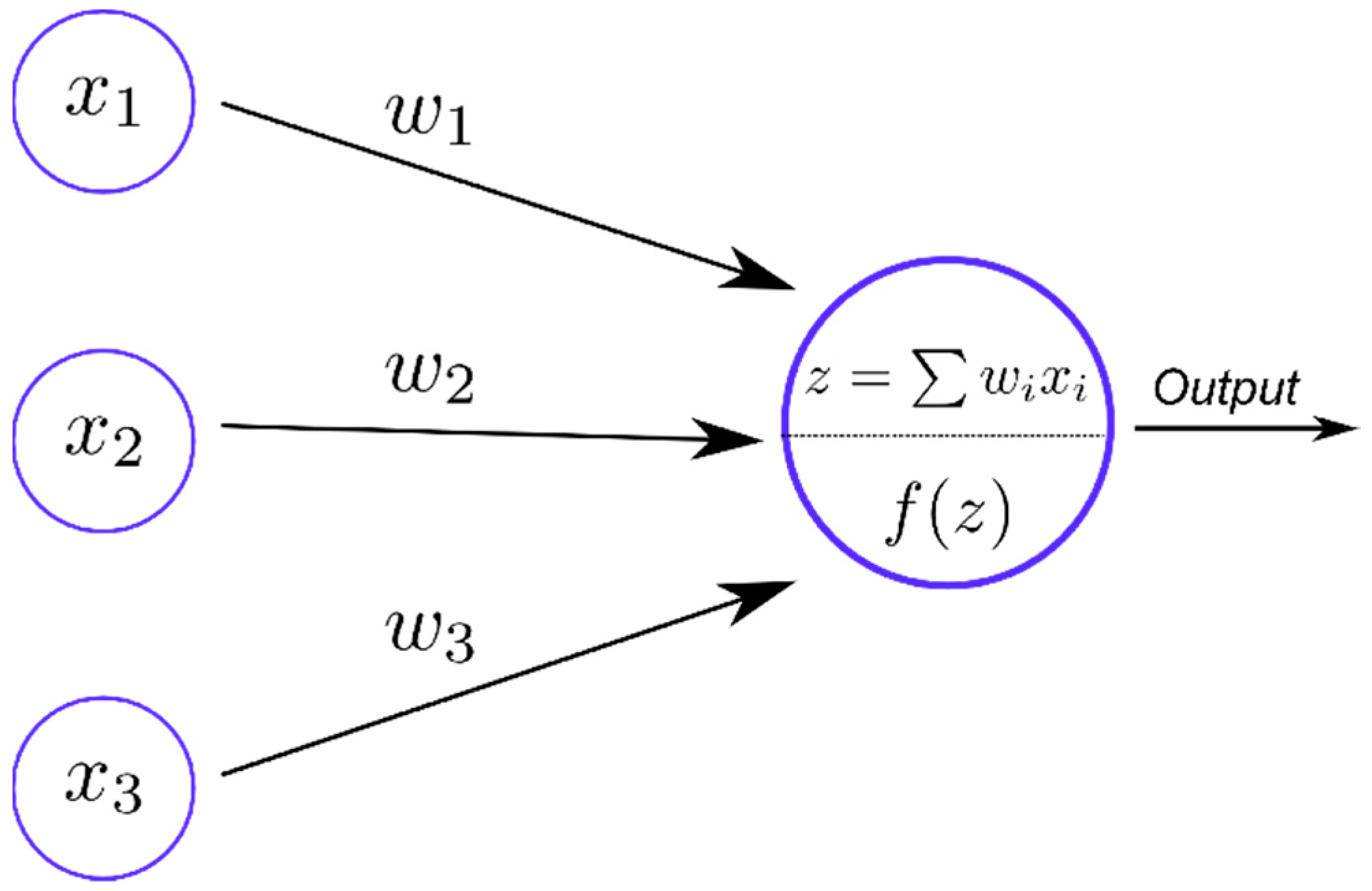
ANNs consist of a collection of basic units called neurons arranged in layers (Figure 7). The first (left) layer is the input layer and the last (right) layer is the output layer. The layers in between are hidden layers. A neural network can have zero or more hidden layers. In a feedforward neural network, the neurons in one layer are connected to the neurons in the next layer and the information flows forward from the input to the output through the hidden layers. When there are many hidden layers, the network is called a deep neural network (DNN). The connections between the neurons are called synapses. A neuron, the basic building block of ANNs, consists of a set of input values, $x_i,i=1,\dots ,n$, a set of weights, $w_i,i=1,\dots ,n$, and a transfer (or activation) function, f (see Figure 8). A linear transformation consisting of the weighted sum of all the inputs, ${\displaystyle \sum w_i}{x}_i$, and a bias, b, is calculated as:

$$z=b+{\displaystyle \sum _{i=1}^n{w}_i}{x}_i$$

(8)

for each neuron. The output, h, is calculated from this neuron through the (usually) nonlinear transfer function, f(z). Typically, each neuron in a given layer has the same transfer function and for each neuron, i, in that layer, the output is calculated as h_i = f(z_i), where is z_i calculated using Equation (8). The outputs serve as the inputs for each of the neurons in the next layer, which can use a different or the same transfer function. This process is continued until the output layer is reached where the neurons compute the output variables, $y_i,i=1,\dots ,p$ (p is the number of outputs). For a binary classifier, there is usually only one neuron in the output layer and therefore p is taken to be unity. However, two neurons can also be used for binary classification [23].

In supervised learning, the training data (input data and the corresponding output data) is used to train the ANN model. The training starts with an initial assumption on the weights w_i. The input data is processed by the ANN and output is predicted. The error between the predicted outputs and the known outputs is calculated using a cost (or loss) function which can be the sum of the squares of the errors between predicted and observed outputs, for example. Since the predicted values depend on the weights and biases, it is clear that the loss function, E, is also a function of the weights and biases for a given set of training data, i.e., $E=E(w_i,b)$. By absorbing the bias b into the weights as an additional parameter, E can be assumed to be a function of only the weights w_i. If the error is not acceptable, the weights are updated through various methods. One approach is the gradient descent method, where the weight updates are computed using the derivatives of the error function with respect to the weights:

$$w_i^{j+1}=w_i^j-\eta {\frac{\partial E}{\partial w_i}|}^j$$

(9)

In Equation (9), the superscript j indicates the jth iteration and η is the learning rate that is used to control the magnitudes of the corrections applied to w_i. Too large a value of η will lead to convergence issues and too small a value increases the computational time and cost. The updated weights are again used for predictions and calculating the error in predictions. This process is repeated until the error is less than a preselected value or a maximum number of iterations has been reached. Although Equation (9) captures the essence of weight updates, in a typical ANN with multiple hidden layers, the gradient calculation is quite complicated and involved. The backpropagation algorithm may be used to compute these gradients. In the standard backpropagation algorithm, the learning rate is kept constant. A modification of this algorithm, called the resilient backpropagation algorithm, uses separate learning rates for each weight and, in addition, these rates can be altered during the training process to accelerate the convergence. Furthermore, the adjustments to weights do not include the partial derivatives of the error function with respect to weights. Instead, only the signs of the derivatives are used in place of the derivatives [31]. In the present work, the resilient backpropagation algorithm was used for updating the weights.

When the training is complete, the performance of the model is evaluated using test data with known outputs. Additional cross-validation methods are also used to further evaluate the model performance. If the predictions from the test data and cross-validations are satisfactory, the ANN model is used for predictive purposes on new sets of input data.

4. ANN Model for Chatter Prediction

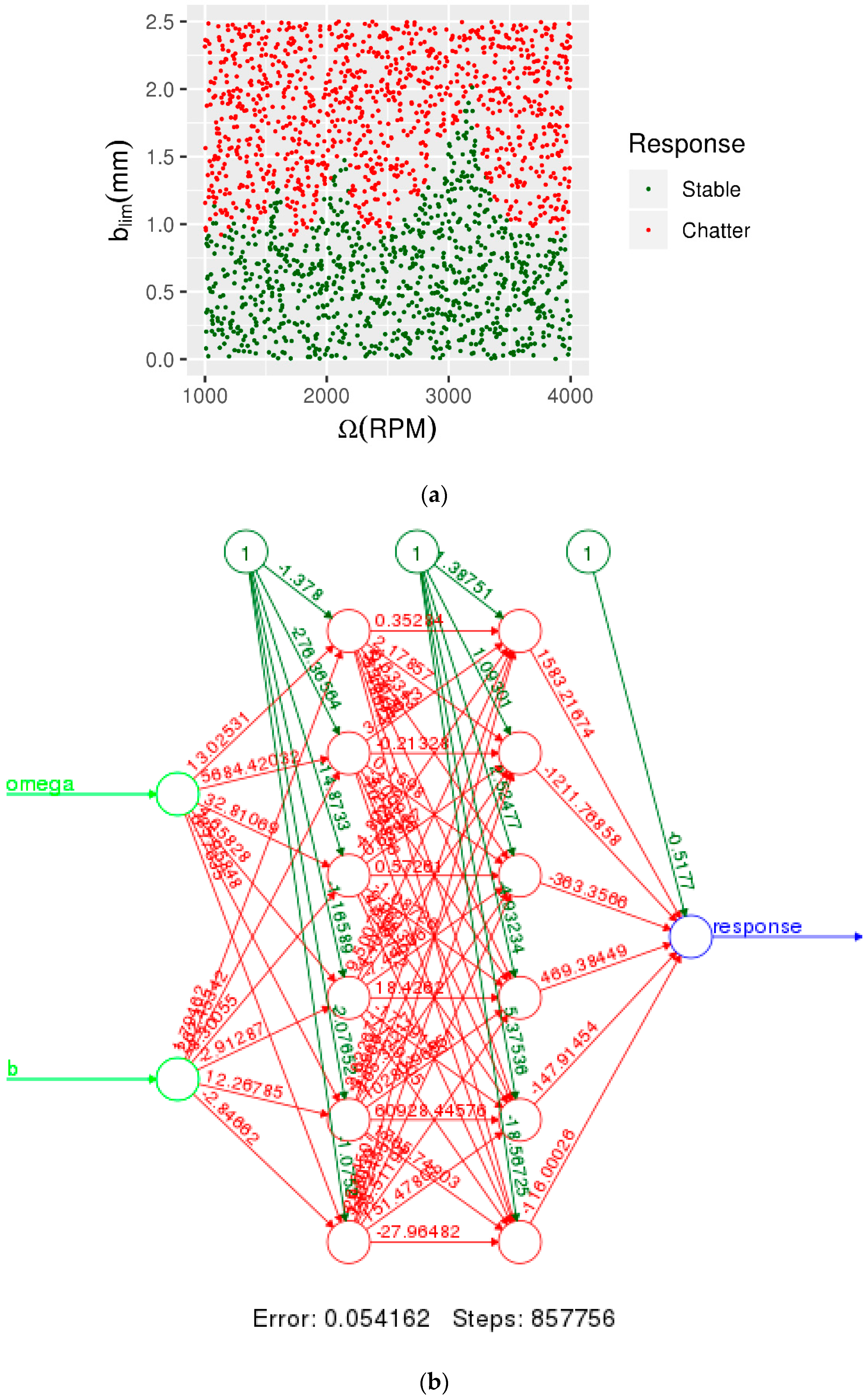
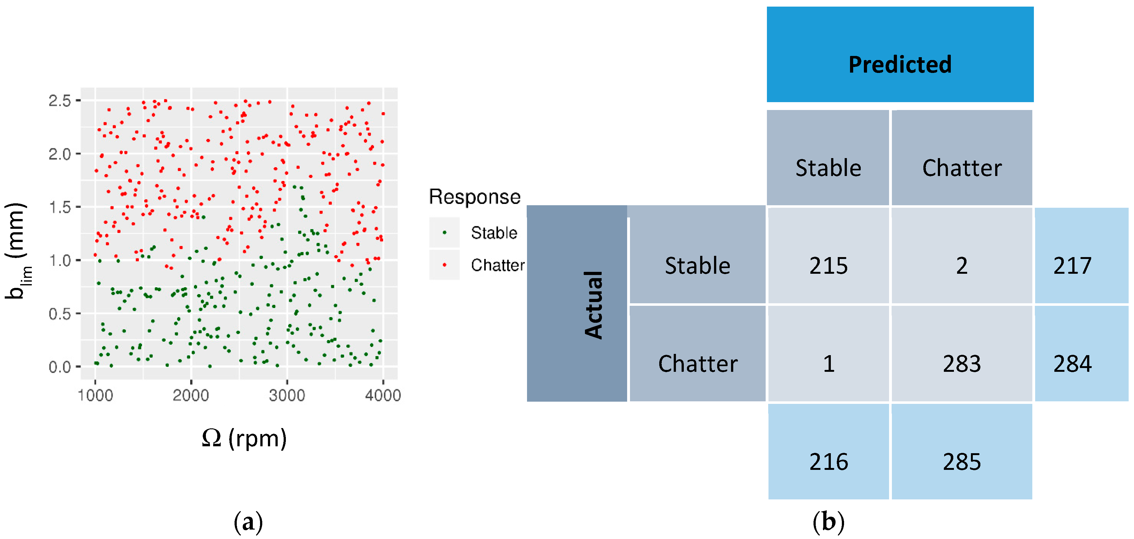
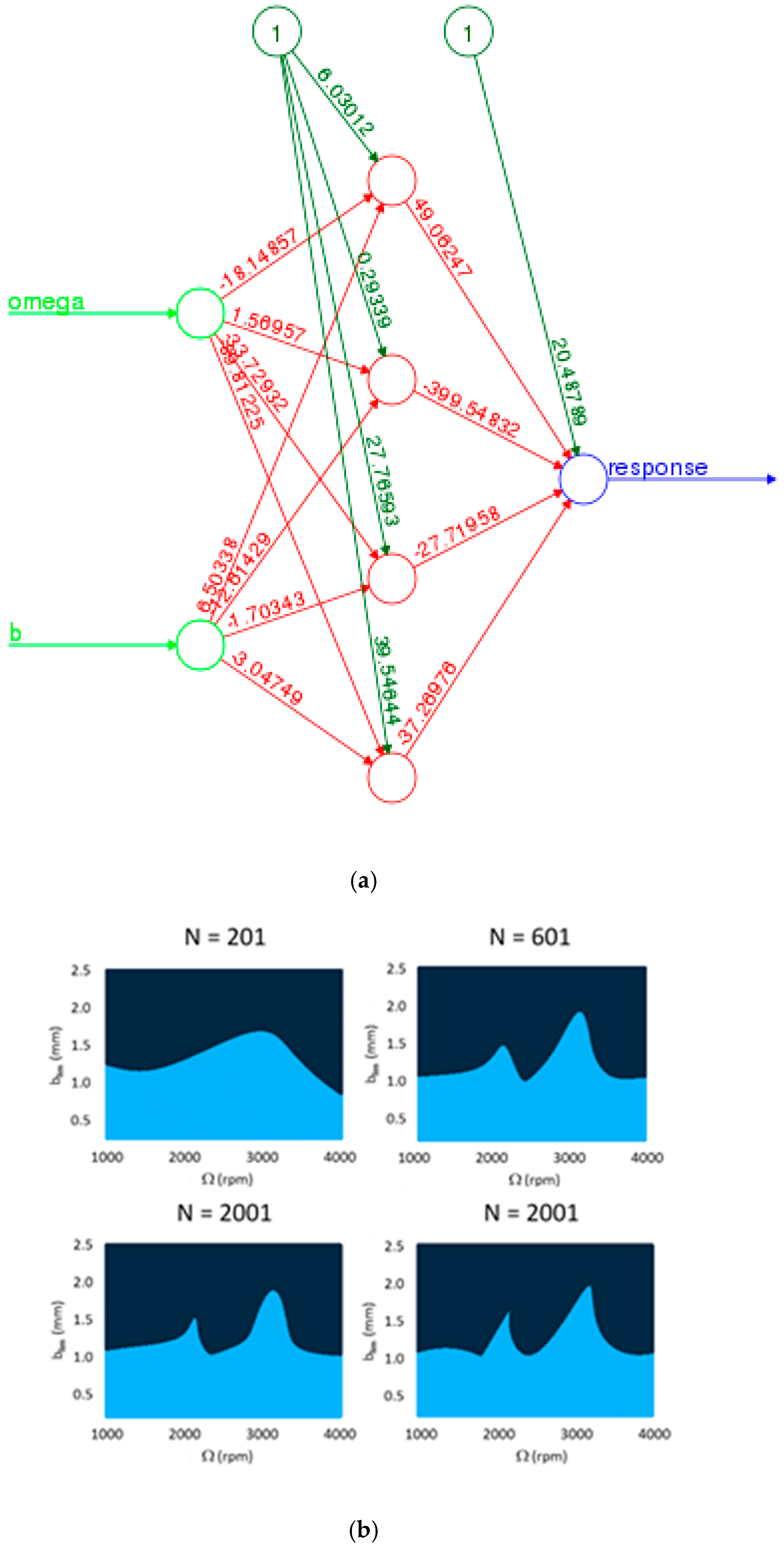
In this work the R neural net package, neuralnet [31], was used to build the ANN model. The input parameters for the neural network were the spindle speed and limiting chip width, see Figure 9. The data set for training and testing was obtained from the stability algorithm described in Section 2. The corresponding model parameters were: k = 1 × 10⁶ N/m, c = 315 N-s/m, m = 2.5 kg, K_s = 700 N/mm², and β = 70 deg. The data set was generated by considering uniformly distributed random values for the pairs (Ω, b_lim) in the range of 1000 rpm to 4000 rpm and 0 mm to 2.5 mm. For each set of values, the cut was labeled as stable or unstable (chatter) using the stability limit. The total number of points in the training set was varied to evaluate the predictive capability on the ANN model. The training and test sets were first rescaled using the max-min normalization method. The value, x, for each of the inputs was mapped to the range [0, 1] through the transformation $(x-x_{min})/(x_{max}-x_{min})$. Since there were no outliers in the input data, this rescaling method was acceptable. The normalized training data was used to train the ANN model. The non-normalized training set consisting of 2001 randomly generated points is shown in Figure 9a. The activation function for the neural network considered in the present work is taken to be the binary logistic function with output between 0 and 1. Output less than 0.5 is taken to be stable and greater than or equal to 0.5 is taken to indicate chatter. The cross entropy loss function is used for E [32]. Furthermore, two hidden layers were considered with six neurons in each layer. The trained neural network with the corresponding weights is shown in Figure 9b.

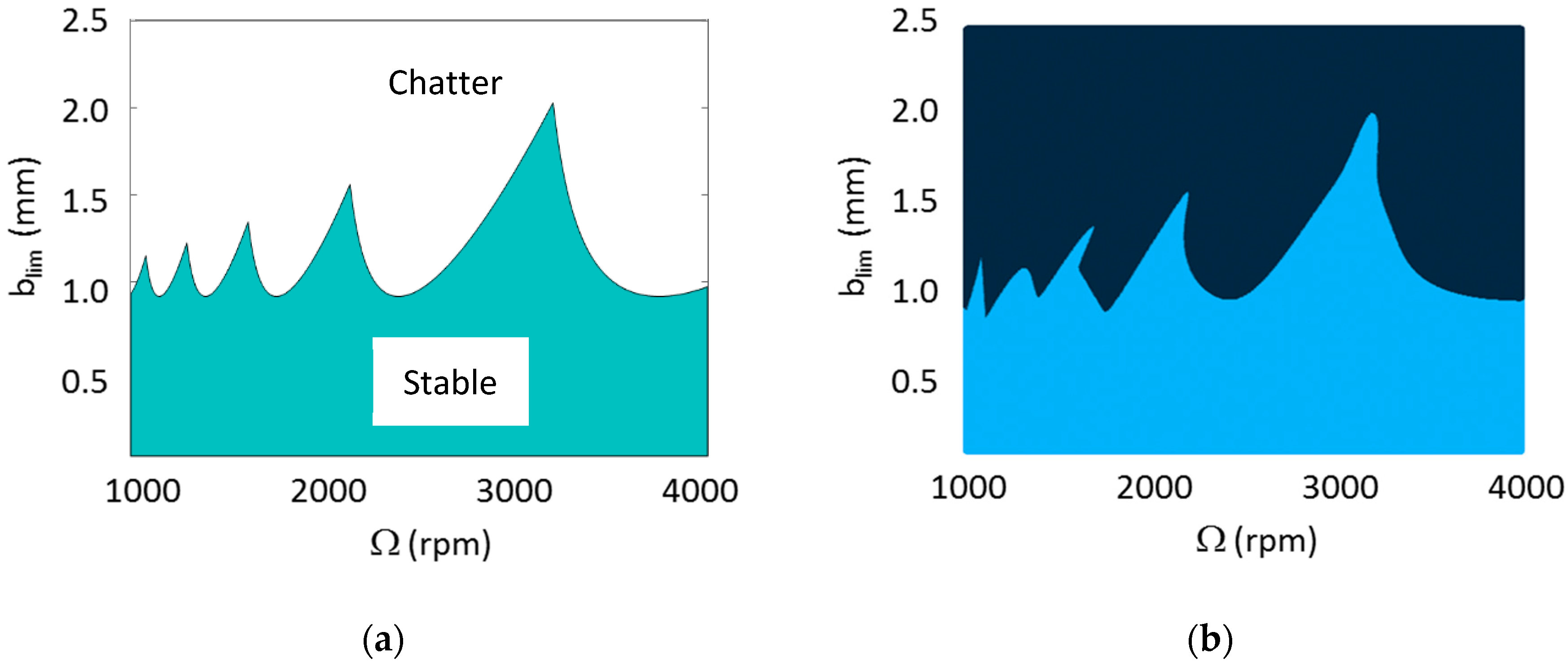
The actual decision boundary and the predicted decision boundaries are shown Figure 10. As the figures indicate, the decision boundary is reasonably reproduced by the ANN model. However, for the points near the lobe peaks and some troughs, the predicted boundary is not accurate. It is to be expected then, that when the model is used for predictive purposes, the predictions may not be accurate when the input data is near these peaks and troughs. However, away from these locations, the accuracy of the predictions can be expected to be high. This is confirmed by evaluating the ANN model using a test set. The predictions by the ANN model on the test set are shown in Figure 11. The test set consists of 501 points randomly distributed in the feature space, see Figure 11a. The ANN model predictions are shown as a confusion matrix in Figure 11b. Only three points out of 501 are misidentified with two false negatives and one false positive (with respect to chatter). The accuracy of the model is 498/501 = 99.4%.

ANN models trained with a fewer number of points or with a single hidden layer were found to be less accurate. In Figure 12a, a single hidden layer neural network with four neurons is shown. The decision boundaries predicted by this model for different numbers of total data points in the training set are shown in Figure 12b. Clearly, the predicted decision boundaries differ from the actual boundary with many of the lobes missing altogether. Therefore, predictions for input data near the actual decision boundary will be inaccurate.

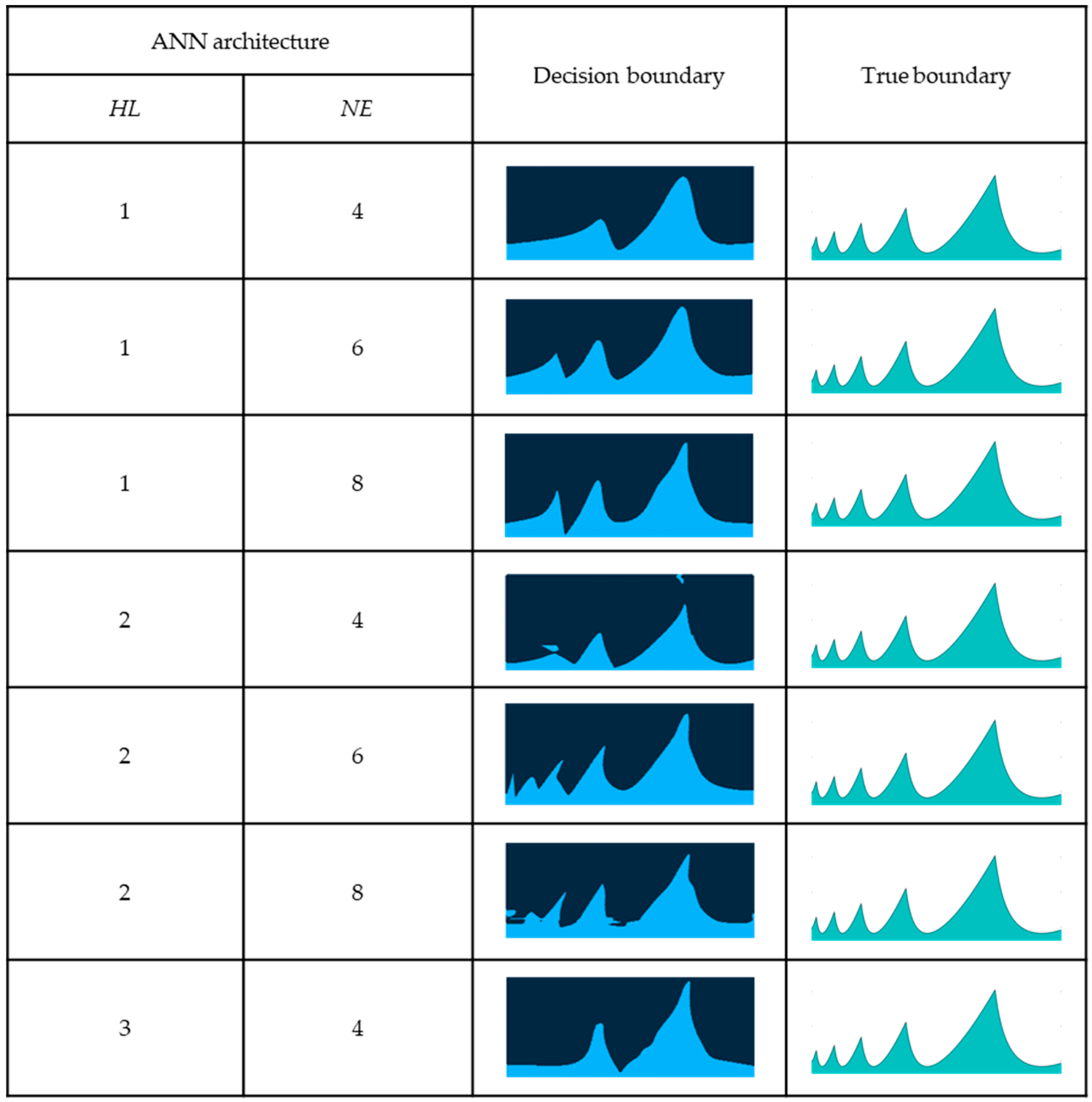
To further examine the sensitivity of the ANN performance to its architecture, seven ANNs were evaluated with different numbers of hidden layers, HL, and neurons, NE, where HL was varied from 1 to 3 and NE from 4 to 8. The decision boundary for each architecture was calculated by considering an evenly spaced grid in the (Ω, b_lim) domain. This domain was divided into a fine grid consisting of 1001 equispaced points in each direction for a total of 1,002,001 points. The results are presented in Figure 13 in the form of various decision boundaries obtained by the predictions of the trained ANN models on these points. Visual comparison to the true boundary demonstrates that the model architecture is closely related to the model accuracy. Of the seven architectures considered, the two hidden layer ANN with six neurons per layer best replicates the true stability boundary. Interestingly, the other two architectures with two hidden layers either did not converge in the specified number of epochs or required adjustments to the stopping criterion. As expected, the training time increased with increasing complexity of the ANN architecture. The two and three hidden layer models required one to three hours using a standard laptop with 8 GB RAM.

5. Conclusions

This paper provided an analysis of the application of artificial neural networks (ANN) to modeling stability behavior in turning. The physics-based, analytical stability limit was used to generate a data set that trained the ANN. It was observed that the number and distribution of training points influence the ability of the ANN model to capture the smaller, more closely spaced lobes that occur at lower spindle speeds. Overall, the ANN is successful (>90% accuracy) at predicting the stability behavior after appropriate training. Deep and narrow ANNs were found to be more accurate than shallow and wide ANNs. A sensitivity study showed that the ANN performance is closely linked to the selected number of hidden layers and neurons per layer. Future work will include incorporating experimental data into the ANN models to augment the data obtained from the physics-based models.

References

- Siddhpura, M.; Paurobally, R. A review of chatter vibration research in turning. Int. J. Mach. Tools Manuf. 2012, 61, 27–47. [Google Scholar] [CrossRef]
- Chanda, A.; Dwivedy, S.K. Nonlinear dynamic analysis of flexible workpiece and tool in turning operation with delay and internal resonance. J. Sound Vib. 2018, 434, 358–378. [Google Scholar] [CrossRef]
- Copenhaver, R.; Schmitz, T.; Smith, S. Stability analysis of modulated tool path turning. Cirp Ann. Manuf. Technol. 2018, 67, 49–52. [Google Scholar] [CrossRef]
- Filippov, A.V.; Rubtsov, V.E.; Tarasov, S.Y.; Podgornykh, O.A.; Shamarin, N.N. Detecting transition to chatter mode in peakless tool turning by monitoring vibration and acoustic emission signals. Int. J. Adv. Manuf. Technol. 2018, 95, 157–169. [Google Scholar] [CrossRef]
- Gerasimenko, A.; Guskov, M.; Gouskov, A.; Lorong, P.; Shokhin, A. Analytical modeling of a thin-walled cylindrical workpiece during the turning process. Stability analysis of a cutting process. J. Vibroengineering 2017, 19, 5825–5841. [Google Scholar] [CrossRef] [Green Version]
- Gouskov, A.M.; Guskov, M.A.; Tung, D.D.; Panovko, G.Y. Modeling and investigation of the stability of a multicutter turning process by a trace. J. Mach. Manuf. Reliab. 2018, 47, 317–323. [Google Scholar] [CrossRef]
- Gyebrószki, G.; Bachrathy, D.; Csernák, G.; Stepan, G. Stability of turning processes for periodic chip formation. Adv. Manuf. 2018, 6, 345–353. [Google Scholar] [CrossRef] [Green Version]
- Hajdu, D.; Insperger, T.; Stepan, G. Robust stability analysis of machining operations. Int. J. Adv. Manuf. Technol. 2017, 88, 45–54. [Google Scholar] [CrossRef]
- Huang, X.; Hu, M.; Zhang, Y.; Lv, C. Probabilistic analysis of chatter stability in turning. Int. J. Adv. Manuf. Technol. 2016, 87, 3225–3232. [Google Scholar] [CrossRef]
- Mousavi, S.; Gagnol, V.; Bouzgarrou, B.C.; Ray, P. Dynamic modeling and stability prediction in robotic machining. Int. J. Adv. Manuf. Technol. 2017, 88, 3053–3065. [Google Scholar] [CrossRef]
- Liu, Y.; Li, T.X.; Liu, K.; Zhang, Y.M. Chatter reliability prediction of turning process system with uncertainties. Mech. Syst. Signal Process. 2016, 66–67, 232–247. [Google Scholar] [CrossRef]
- Khasawneh, F.A.; Munch, E. Chatter detection in turning using persistent homology. Mech. Syst. Signal Process. 2016, 70–71, 527–541. [Google Scholar] [CrossRef]
- Jiménez Cortadi, A.; Irigoyen, I.; Boto, F.; Sierra, B.; Suárez, A.; Galar, D. A statistical data-based approach to instability detection and wear prediction in radial turning processes. Eksploat. I Niezawodn. Maint. Reliab. 2018, 20, 405–412. [Google Scholar] [CrossRef]
- Jasiewicz, M.; Powalka, B. Prediction of turning stability using receptance coupling. AIP Conf. Proc. 2018, 1922, 100005. [Google Scholar] [CrossRef]
- Lu, K.; Lian, Z.; Gu, F.; Liu, H. Model-based chatter stability prediction and detection for the turning of a flexible workpiece. Mech. Syst. Signal Process. 2018, 100, 814–826. [Google Scholar] [CrossRef]
- Tyler, C.; Troutman, J.R.; Schmitz, T. A coupled dynamics, multiple degree of freedom process damping model, Part 1: Turning. Precis. Eng. 2016, 46, 65–72. [Google Scholar] [CrossRef]
- Ahmad, N.; Janahiraman, T.V.; Tarlochan, F. Modeling of surface roughness in turning operation using extreme learning machine. Arab. J. Sci. Eng. 2015, 40, 595–602. [Google Scholar] [CrossRef]
- Lamraoui, M.; Barakat, M.; Thomas, M.; El Badaoui, M. Chatter detection in milling machines by neural network classification and feature selection. J. Vib. Control 2015, 21, 1251–1266. [Google Scholar] [CrossRef]
- Gupta, A.K.; Guntuku, S.C.; Desu, R.K.; Balu, A. Optimisation of turning parameters by integrating genetic algorithm with support vector regression and artificial neural networks. Int. J. Adv. Manuf. Technol. 2015, 77, 331–339. [Google Scholar] [CrossRef]
- Jurkovic, Z.; Cukor, G.; Brezocnik, M.; Brajkovic, T. A comparison of machine learning methods for cutting parameters prediction in high speed turning process. J. Intell. Manuf. 2018, 29, 1683–1693. [Google Scholar] [CrossRef]
- Khasawneh, F.A.; Munch, E.; Perea, J.A. Chatter classification in turning using machine learning and topological data analysis. IFAC Pap. 2018, 51, 195–200. [Google Scholar] [CrossRef]
- Yao, Z.; Mei, D.; Chen, Z. On-line chatter detection and identification based on wavelet and support vector machine. J. Mater. Process. Technol. 2010, 210, 713–719. [Google Scholar] [CrossRef]
- Zagórski, I.; Kulisz, M.; Semeniuk, A.; Malec, A. Artificial neural network modelling of vibration in the milling of AZ91D alloy. Adv. Sci. Technol. Res. J. 2017, 11, 261–269. [Google Scholar] [CrossRef]
- Kumar, S.; Singh, B. Ascertaining of chatter stability using wavelet denoising and artificial neural network. Proc. Inst. Mech. Eng. Part C 2018, 233, 39–62. [Google Scholar] [CrossRef]
- Schmitz, T.; Smith, K.S. Machining Dynamics: Frequency Response to Improved Productivity, 2nd ed.; Springer: New York, NY, USA, 2019. [Google Scholar]
- Tlusty, G. Manufacturing Equipment and Processes; Prentice-Hall: Upper Saddle River, NJ, USA, 2000. [Google Scholar]
- Karandikar, J.; Zapata, R.; Schmitz, T. Incorporating stability, surface location error, tool wear, and uncertainty in the milling super diagram. Trans. NAMRI/SME 2010, 38, 229–236. [Google Scholar]
- Schmitz, T.; Karandikar, J.; Kim, N.H.; Abbas, A. Uncertainty in machining: Workshop summary and contributions. J. Manuf. Sci. Eng. 2011, 133, 051009. [Google Scholar] [CrossRef]
- Schmitz, T.; Ziegert, J.; Canning, J.S.; Zapata, R. Case study: A comparison of error sources in milling. Precis. Eng. 2008, 32, 126–133. [Google Scholar] [CrossRef]
- Kim, H.S.; Schmitz, T. Bivariate uncertainty analysis for impact testing. Meas. Sci. Technol. 2007, 18, 3565–3571. [Google Scholar] [CrossRef]
- Fritsch, S.; Guenther, F.; Guenther, M.F. Package ‘neuralnet’. Training of Neural Networks. Available online: ftp://64.50.236.52/.1/cran/web/packages/neuralnet/neuralnet.pdf (accessed on 31 May 2019).
- Intrator, O.; Intrator, N. Interpreting neural-network results: A simulation study. Comput. Stat. Data Anal. 2001, 37, 373–393. [Google Scholar] [CrossRef]
Figure 1.
Orthogonal cutting operation showing the cutting force with its normal and tangential components [25]. Adapted with permission from Springer Nature, Machining Dynamics: Frequency Response to Improved Productivity by Schmitz, T.L. and Smith, K.S., 2019.
Figure 2.
Description of regenerative chatter in turning. Initial tool deflections are copied onto the workpiece surface and are encountered in subsequent revolutions. This varies the chip thickness and cutting force which, in turn, affects the resulting tool deflections [25]. Adapted with permission from Springer Nature, Machining Dynamics: Frequency Response to Improved Productivity by Schmitz, T.L. and Smith, K.S., 2019.
Figure 3.
Depiction of turning where the surface from the previous revolution, shown to the left of the tool, is removed by the vibrating cutter to produce a new wavy surface to the right of the tool [25]. Adapted with permission from Springer Nature, Machining Dynamics: Frequency Response to Improved Productivity by Schmitz, T.L. and Smith, K.S., 2019.
Figure 4.
The figure demonstrates the instantaneous chip thickness calculation. It depends on the mean feed per revolution, the current deflection, and the vibration during the previous revolution of the workpiece (to the left of the tool) [25]. Adapted with permission from Springer Nature, Machining Dynamics: Frequency Response to Improved Productivity by Schmitz, T.L. and Smith, K.S., 2019.
Figure 5.
The surface waviness between revolutions is in phase. Negligible chip thickness variation is obtained [25]. Adapted with permission from Springer Nature, Machining Dynamics: Frequency Response to Improved Productivity by Schmitz, T.L. and Smith, K.S., 2019.
Figure 6.
Less favorable phase relationship between revolutions yields significant chip thickness variation [25]. Adapted with permission from Springer Nature, Machining Dynamics: Frequency Response to Improved Productivity by Schmitz, T.L. and Smith, K.S., 2019.
Figure 7.
An example of an artificial neural network (ANN). This ANN has four inputs (features), one hidden layer with three neurons, and two outputs.
Figure 8.
A single neuron consists of the inputs xi, the weights wi, and the transfer function f(z), which produces the scalar value h. Note that z is defined with the bias b absorbed into the summation by setting x0 = 1 and w0 = b.
Figure 9.
(a) The training set consisting of 2001 points was used to train, (b) a two hidden layer artificial neural network.
Figure 10.
The decision boundary separates the stable region from the chatter region. (a) The actual boundary, and (b) the predicted decision boundary.
Figure 11.
(a) The test data set consisting of 501 points, and (b) the predictions by the trained neural network on this data (shown as a confusion matrix).
Figure 12.
(a) One hidden layer neural network with four neurons. (b) The decision boundaries predicted by the neural network. The decision boundaries in the top row correspond to 201 and 601 points in the training set. The bottom two correspond to 2001 points each, but with two different random distributions.
Figure 13.
Results for study of ANN sensitivity to architecture.
© 2019 by the authors. Licensee MDPI, Basel, Switzerland. This article is an open access article distributed under the terms and conditions of the Creative Commons Attribution (CC BY) license (http://creativecommons.org/licenses/by/4.0/).
Share and Cite
MDPI and ACS Style
Cherukuri, H.; Perez-Bernabeu, E.; Selles, M.; Schmitz, T. Machining Chatter Prediction Using a Data Learning Model. J. Manuf. Mater. Process. 2019, 3, 45. https://doi.org/10.3390/jmmp3020045
AMA Style
Cherukuri H, Perez-Bernabeu E, Selles M, Schmitz T. Machining Chatter Prediction Using a Data Learning Model. Journal of Manufacturing and Materials Processing. 2019; 3(2):45. https://doi.org/10.3390/jmmp3020045
Chicago/Turabian StyleCherukuri, Harish, Elena Perez-Bernabeu, Miguel Selles, and Tony Schmitz. 2019. "Machining Chatter Prediction Using a Data Learning Model" Journal of Manufacturing and Materials Processing 3, no. 2: 45. https://doi.org/10.3390/jmmp3020045