
Magnetoencephalography Atlas Viewer for Dipole Localization and Viewing
 , , and
Abstract
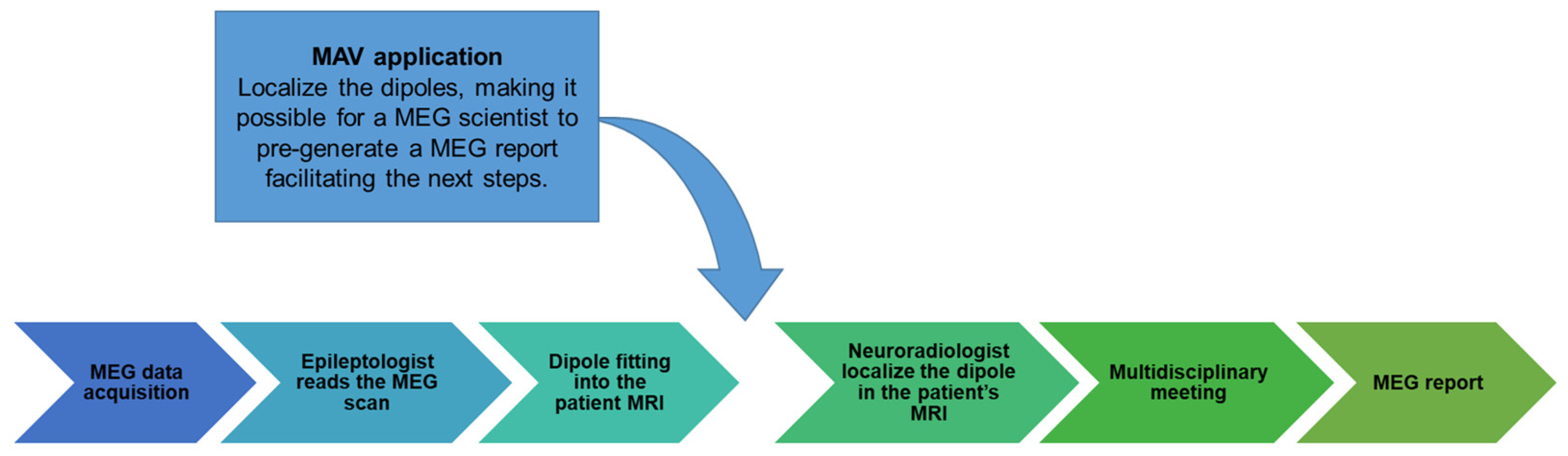
:1. Introduction
2. Materials and Methods
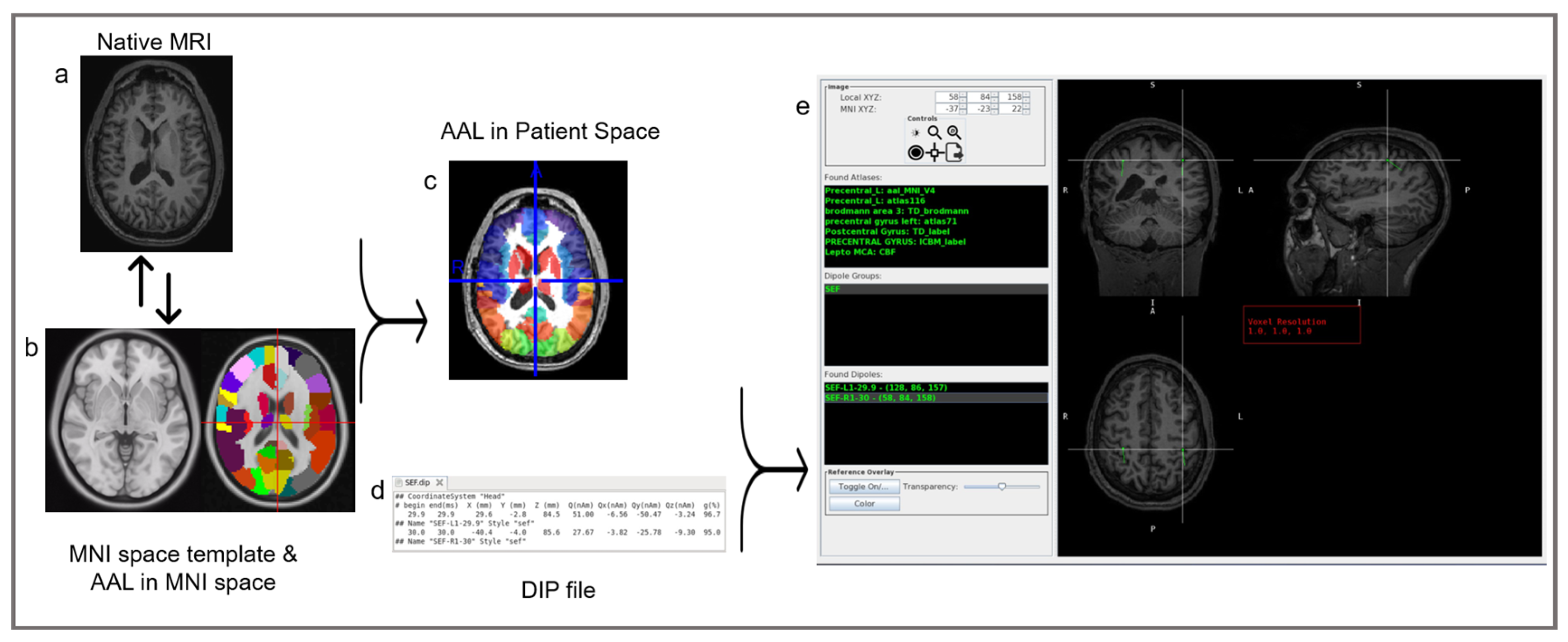
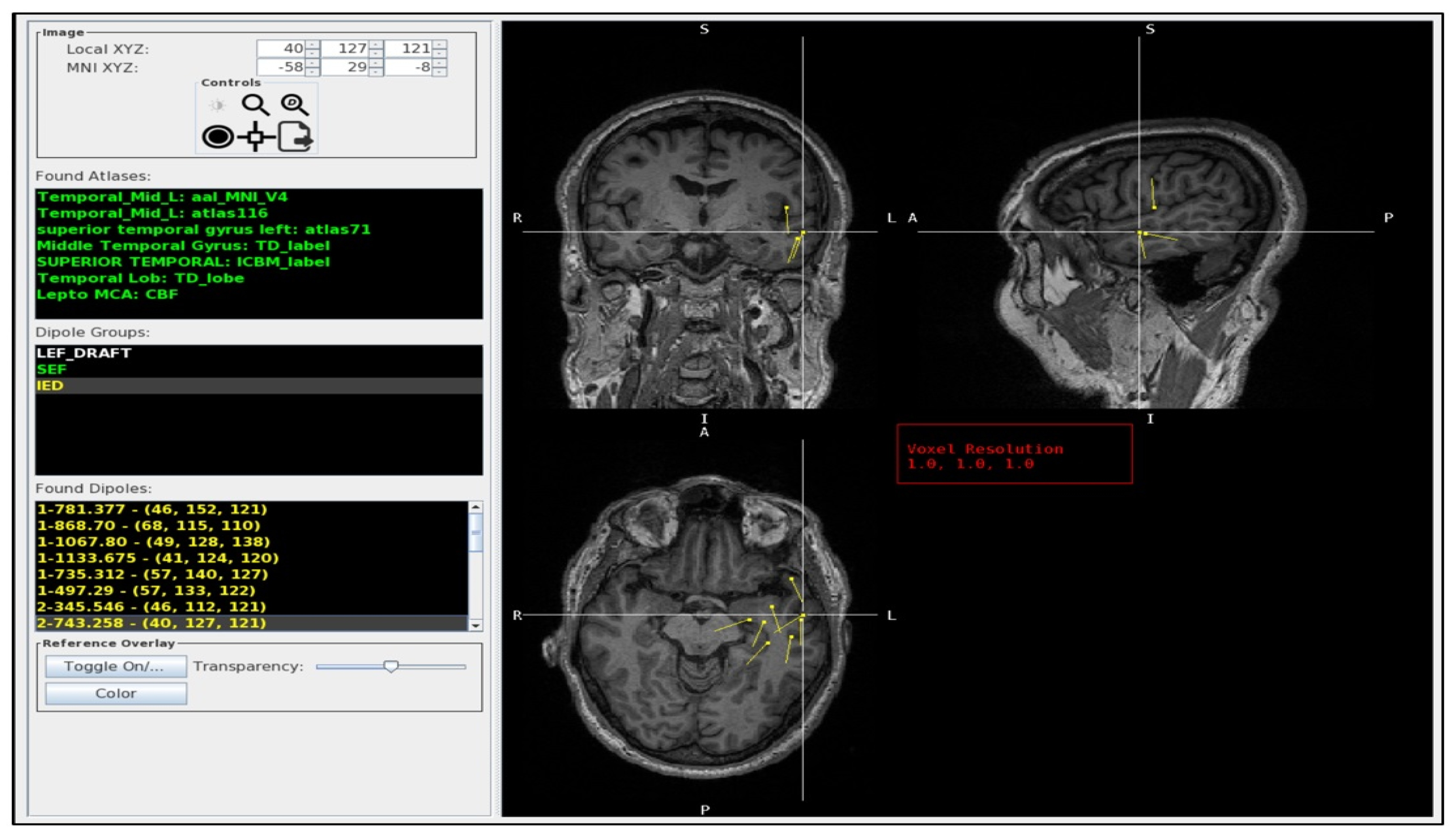
2.1. The MEG Atlas Viewer
2.2. Atlases
2.3. Normalization
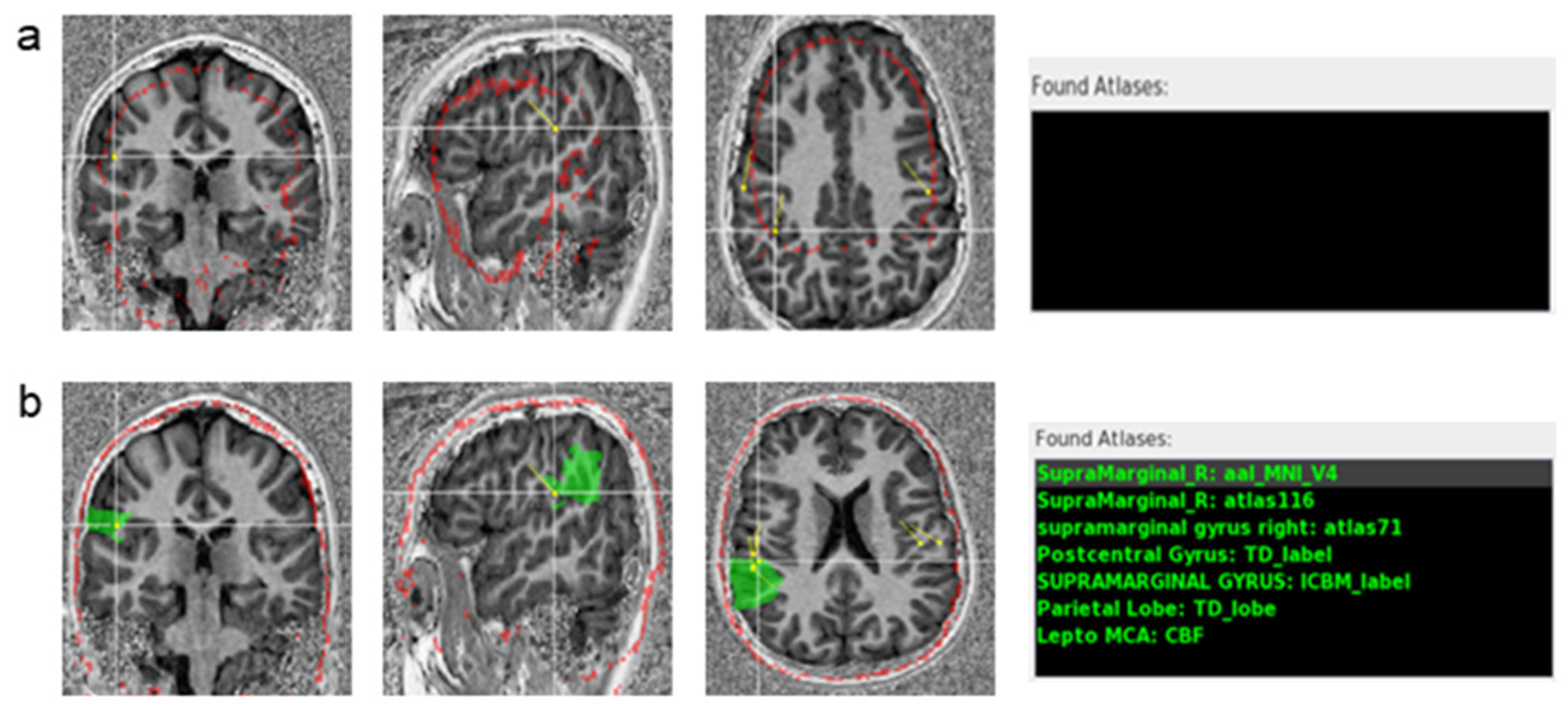
2.4. Atlas Normalization Validation
2.5. MEG Dipoles
2.6. Testing the Performance of the Viewer
3. Results
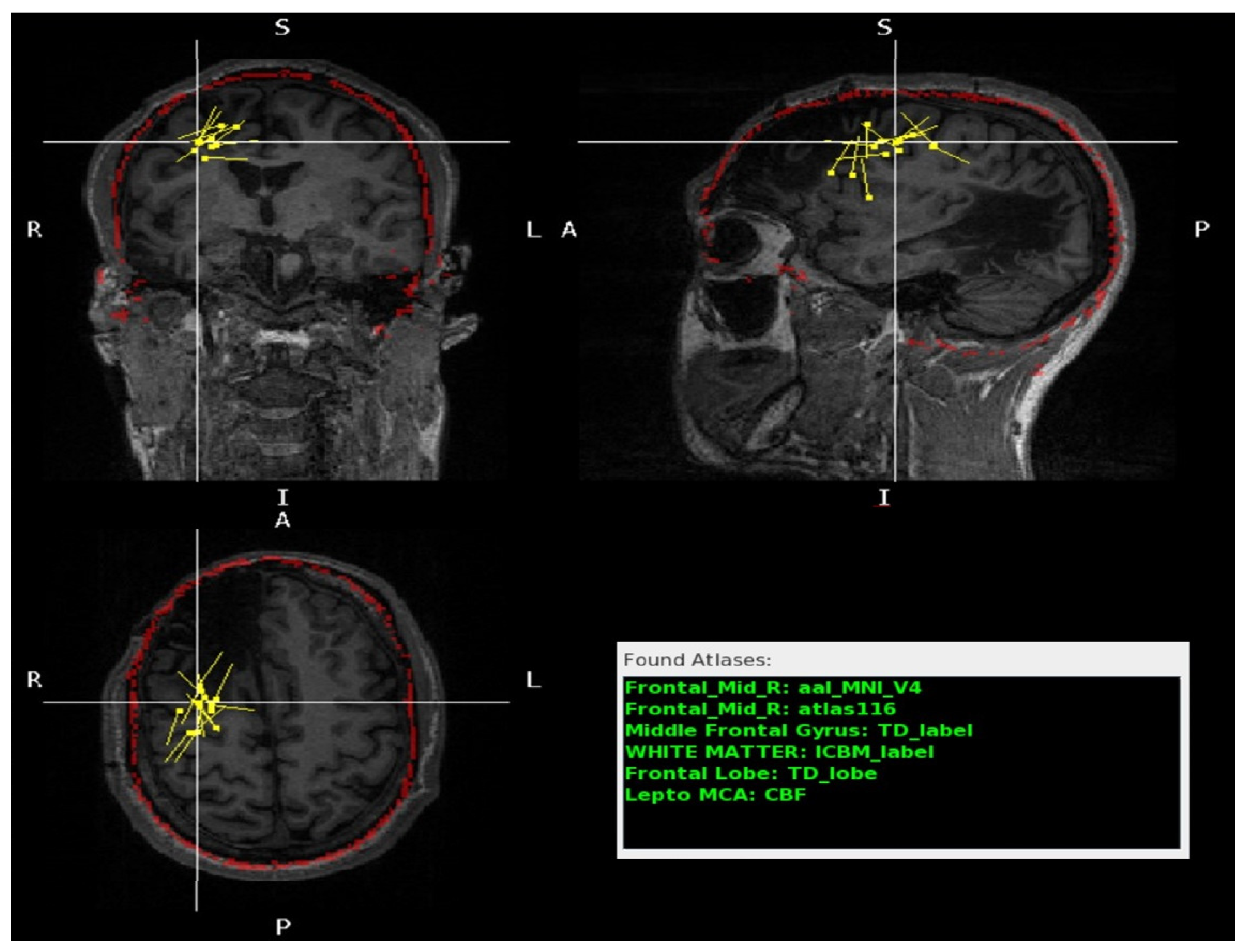
3.1. Usage of the Program Tools
3.2. Performance of the Program
4. Discussion
5. Conclusions
Supplementary Materials
Author Contributions
Funding
Institutional Review Board Statement
Informed Consent Statement
Data Availability Statement
Acknowledgments
Conflicts of Interest
Abbreviations
| AAL | Automated Anatomical Labeling |
| CAT12 | version 12 of the Computational Anatomy Toolbox |
| FLIRT | FMRIB’s Linear Image Registration Tool |
| MEG | Magnetoencephalography |
References
- Hämäläinen, M.; Hari, R.; Ilmoniemi, R.J.; Knuutila, J.; Lounasmaa, O.V. Magnetoencephalography—Theory, instrumentation, and applications to noninvasive studies of the working human brain. Rev. Mod. Phys. 1993, 65, 413. [Google Scholar] [CrossRef]
- Murakami, S.; Okada, Y. Contributions of principal neocortical neurons to magnetoencephalography and electroencephalography signals. J. Physiol. 2006, 575, 925–936. [Google Scholar] [CrossRef]
- Hari, R.; Baillet, S.; Barnes, G.; Burgess, R.; Forss, N.; Gross, J.; Hämäläinen, M.; Jensen, O.; Kakigi, R.; Mauguière, F.; et al. IFCN-endorsed practical guidelines for clinical magnetoencephalography (MEG). Clin. Neurophysiol. 2018, 129, 1720–1747. [Google Scholar] [CrossRef]
- Stufflebeam, S.M.; Tanaka, N.; Ahlfors, S.P. Clinical applications of magnetoencephalography. Hum. Brain Mapp. 2009, 30, 1813–1823. [Google Scholar] [CrossRef]
- Kim, J.A.; Davis, K.D. Magnetoencephalography: Physics, techniques, and applications in the basic and clinical neurosciences. J. Neurophysiol. 2021, 125, 938–956. [Google Scholar] [CrossRef]
- Burgess, R.C.; Funke, M.E.; Bowyer, S.M.; Lewine, J.D.; Kirsch, H.E.; Bagić, A.I.; ACMEGS Clinical Practice Guideline (CPG) Committee. American Clinical Magnetoencephalography Society Clinical Practice Guideline 2: Presurgical functional brain mapping using magnetic evoked fields. J. Clin. Neurophysiol. 2011, 28, 355. [Google Scholar] [CrossRef]
- Bowyer, S.M.; Pang, E.W.; Huang, M.; Papanicolaou, A.C.; Lee, R.R. Presurgical functional mapping with magnetoencephalography. Neuroimaging Clin. 2020, 30, 159–174. [Google Scholar] [CrossRef]
- Fred, A.L.; Kumar, S.N.; Kumar Haridhas, A.; Ghosh, S.; Purushothaman Bhuvana, H.; Sim, W.K.J.; Vimalan, V.; Givo, F.A.S.; Jousmäki, V.; Padmanabhan, P.; et al. A Brief Introduction to Magnetoencephalography (MEG) and Its Clinical Applications. Brain Sci. 2022, 12, 788. [Google Scholar] [CrossRef]
- Murakami, H.; Wang, Z.I.; Marashly, A.; Krishnan, B.; Prayson, R.A.; Kakisaka, Y.; Mosher, J.C.; Bulacio, J.; Gonzalez-Martinez, J.A.; Bingaman, W.E. Correlating magnetoencephalography to stereo-electroencephalography in patients undergoing epilepsy surgery. Brain 2016, 139, 2935–2947. [Google Scholar] [CrossRef]
- Vadera, S.; Jehi, L.; Burgess, R.C.; Shea, K.; Alexopoulos, A.V.; Mosher, J.; Gonzalez-Martinez, J.; Bingaman, W. Correlation between magnetoencephalography-based “clusterectomy” and postoperative seizure freedom. Neurosurg. Focus 2013, 34, E9. [Google Scholar] [CrossRef]
- Mohamed, I.S.; Toffa, D.H.; Robert, M.; Cossette, P.; Bérubé, A.-A.; Saint-Hilaire, J.-M.; Bouthillier, A.; Nguyen, D.K. Utility of magnetic source imaging in nonlesional focal epilepsy: A prospective study. Neurosurg. Focus 2020, 48, E16. [Google Scholar] [CrossRef]
- Hämäläinen, M.; Huang, M.; Bowyer, S.M. Magnetoencephalography signal processing, forward modeling, inverse source imaging, and coherence analysis. Neuroimaging Clin. 2020, 30, 125–143. [Google Scholar] [CrossRef]
- Ray, A.; Bowyer, S.M. Clinical applications of magnetoencephalography in epilepsy. Ann. Indian Acad. Neurol. 2010, 13, 14. [Google Scholar] [CrossRef]
- Burgess, R.C. MEG for greater sensitivity and more precise localization in epilepsy. Neuroimaging Clin. 2020, 30, 145–158. [Google Scholar] [CrossRef]
- Tenney, J.R.; Fujiwara, H.; Rose, D.F. The value of source localization for clinical magnetoencephalography: Beyond the equivalent current dipole. J. Clin. Neurophysiol. 2020, 37, 537–544. [Google Scholar] [CrossRef]
- Mosher, J.C.; Funke, M.E. Towards Best Practices in Clinical Magnetoencephalography: Patient Preparation and Data Acquisition. J. Clin. Neurophysiol. 2020, 37, 498–507. [Google Scholar] [CrossRef]
- Laohathai, C.; Ebersole, J.S.; Mosher, J.C.; Bagić, A.I.; Sumida, A.; Von Allmen, G.; Funke, M.E. Practical Fundamentals of Clinical MEG Interpretation in Epilepsy. Front. Neurol. 2021, 12, 722986. [Google Scholar] [CrossRef]
- Bagic, A.I.; Knowlton, R.C.; Rose, D.F.; Ebersole, J.S.; ACMEGS Clinical Practice Guideline (CPG) Committee. American clinical magnetoencephalography society clinical practice guideline 1: Recording and analysis of spontaneous cerebral activity. J. Clin. Neurophysiol. 2011, 28, 348–354. [Google Scholar]
- Widjaja, E.; Otsubo, H.; Raybaud, C.; Ochi, A.; Chan, D.; Rutka, J.T.; Snead, O.C.; Halliday, W.; Sakuta, R.; Galicia, E.; et al. Characteristics of MEG and MRI between Taylor’s focal cortical dysplasia (type II) and other cortical dysplasia: Surgical outcome after complete resection of MEG spike source and MR lesion in pediatric cortical dysplasia. Epilepsy Res. 2008, 82, 147–155. [Google Scholar] [CrossRef] [PubMed]
- Burgess, R.C. MEG Reporting. J. Clin. Neurophysiol. 2020, 37, 545–553. [Google Scholar] [CrossRef] [PubMed]
- Bock, E.; Baillet, S. MEG-Clinic: A Comprehensive Software Solution for Routine MEG Analysis. In Proceedings of the 17th International Conference on Biomagnetism Advances in Biomagnetism–Biomag2010, Dubrovnik, Croatia, 28 March–1 April 2010; pp. 128–131. [Google Scholar]
- Capilla, A.; Arana, L.; García-Huéscar, M.; Melcón, M.; Gross, J.; Campo, P. The natural frequencies of the resting human brain: An MEG-based atlas. NeuroImage 2022, 258, 119373. [Google Scholar] [CrossRef]
- Tait, L.; Özkan, A.; Szul, M.J.; Zhang, J. A systematic evaluation of source reconstruction of resting MEG of the human brain with a new high-resolution atlas: Performance, precision, and parcellation. Hum. Brain Mapp. 2021, 42, 4685–4707. [Google Scholar] [CrossRef]
- Hirano, R.; Emura, T.; Nakata, O.; Nakashima, T.; Asai, M.; Kagitani-Shimono, K.; Kishima, H.; Hirata, M. Fully-Automated Spike Detection and Dipole Analysis of Epileptic MEG Using Deep Learning. IEEE Trans. Med. Imaging 2022, 41, 2879–2890. [Google Scholar] [CrossRef]
- Maldjian, J.A.; Laurienti, P.J.; Kraft, R.A.; Burdette, J.H. An automated method for neuroanatomic and cytoarchitectonic atlas-based interrogation of fMRI data sets. Neuroimage 2003, 19, 1233–1239. [Google Scholar] [CrossRef]
- Taylor, K.N.; Joshi, A.A.; Hirfanoglu, T.; Grinenko, O.; Liu, P.; Wang, X.; Gonzalez-Martinez, J.A.; Leahy, R.M.; Mosher, J.C.; Nair, D.R. Validation of semi-automated anatomically labeled SEEG contacts in a brain atlas for mapping connectivity in focal epilepsy. Epilepsia Open 2021, 6, 493–503. [Google Scholar] [CrossRef]
- Antonopoulos, G.; More, S.; Raimondo, F.; Eickhoff, S.B.; Hoffstaedter, F.; Patil, K.R. A systematic comparison of VBM pipelines and their application to age prediction. Neuroimage 2023, 279, 120292. [Google Scholar] [CrossRef]
- Valdés-Hernández, P.A.; von Ellenrieder, N.; Ojeda-Gonzalez, A.; Kochen, S.; Alemán-Gómez, Y.; Muravchik, C.; Valdés-Sosa, P.A. Approximate average head models for EEG source imaging. J. Neurosci. Methods 2009, 185, 125–132. [Google Scholar] [CrossRef]
- Vinding, M.C.; Oostenveld, R. Sharing individualised template MRI data for MEG source reconstruction: A solution for open data while keeping subject confidentiality. NeuroImage 2022, 254, 119165. [Google Scholar] [CrossRef]
- Klein, A.; Andersson, J.; Ardekani, B.A.; Ashburner, J.; Avants, B.; Chiang, M.-C.; Christensen, G.E.; Collins, D.L.; Gee, J.; Hellier, P.; et al. Evaluation of 14 nonlinear deformation algorithms applied to human brain MRI registration. NeuroImage 2009, 46, 786–802. [Google Scholar] [CrossRef] [PubMed]
- Ashburner, J.; Friston, K.J. Nonlinear spatial normalization using basis functions. Hum. Brain Mapp. 1999, 7, 254–266. [Google Scholar] [CrossRef]
- Crinion, J.; Ashburner, J.; Leff, A.; Brett, M.; Price, C.; Friston, K. Spatial normalization of lesioned brains: Performance evaluation and impact on fMRI analyses. NeuroImage 2007, 37, 866–875. [Google Scholar] [CrossRef] [PubMed]
- Jenkinson, M.; Bannister, P.; Brady, M.; Smith, S. Improved Optimization for the Robust and Accurate Linear Registration and Motion Correction of Brain Images. NeuroImage 2002, 17, 825–841. [Google Scholar] [CrossRef] [PubMed]
- Jenkinson, M.; Smith, S. A global optimisation method for robust affine registration of brain images. Med. Image Anal. 2001, 5, 143–156. [Google Scholar] [CrossRef] [PubMed]
- Greve, D.N.; Fischl, B. Accurate and robust brain image alignment using boundary-based registration. NeuroImage 2009, 48, 63–72. [Google Scholar] [CrossRef] [PubMed]
- Woolrich, M.W.; Jbabdi, S.; Patenaude, B.; Chappell, M.; Makni, S.; Behrens, T.; Beckmann, C.; Jenkinson, M.; Smith, S.M. Bayesian analysis of neuroimaging data in FSL. Neuroimage 2009, 45, S173–S186. [Google Scholar] [CrossRef] [PubMed]
- Smith, S.M.; Jenkinson, M.; Woolrich, M.W.; Beckmann, C.F.; Behrens, T.E.; Johansen-Berg, H.; Bannister, P.R.; De Luca, M.; Drobnjak, I.; Flitney, D.E. Advances in functional and structural MR image analysis and implementation as FSL. Neuroimage 2004, 23, S208–S219. [Google Scholar] [CrossRef] [PubMed]
- Jenkinson, M.; Beckmann, C.F.; Behrens, T.E.J.; Woolrich, M.W.; Smith, S.M. FSL. NeuroImage 2012, 62, 782–790. [Google Scholar] [CrossRef] [PubMed]
- Gaser, C.; Dahnke, R.; Thompson, P.M.; Kurth, F.; Luders, E.; Alzheimer’s Disease Neuroimaging Initiative. CAT—A Computational Anatomy Toolbox for the Analysis of Structural MRI Data. Neuroscience, 2022. [Google Scholar] [CrossRef]
- Friston, K.J. Statistical parametric mapping. In Functional Neuroimaging: Technical Foundations; Academic Press: San Diego, CA, USA, 1994; pp. 79–93. [Google Scholar]
- Talairach, J.; Tournoux, P.; Rayport, M. Co-Planar Stereotaxic Atlas of the Human Brain: 3-Dimensional Proportional System: An Approach to Cerebral Imaging; Cambridge University Press: Cambridge, UK, 1988. [Google Scholar]
- Evans, A.C.; Collins, D.L.; Mills, S.R.; Brown, E.D.; Kelly, R.L.; Peters, T.M. 3D statistical neuroanatomical models from 305 MRI volumes. In Proceedings of the 1993 IEEE Conference Record Nuclear Science Symposium and Medical Imaging Conference, San Francisco, CA, USA, 31 October–6 November 1993; pp. 1813–1817. [Google Scholar]
- Brett, M.; Johnsrude, I.S.; Owen, A.M. The problem of functional localization in the human brain. Nat. Rev. Neurosci. 2002, 3, 243–249. [Google Scholar] [CrossRef] [PubMed]
- Evans, A.C.; Marrett, S.; Neelin, P.; Collins, L.; Worsley, K.; Dai, W.; Milot, S.; Meyer, E.; Bub, D. Anatomical mapping of functional activation in stereotactic coordinate space. NeuroImage 1992, 1, 43–53. [Google Scholar] [CrossRef]
- Chau, W.; McIntosh, A.R. The Talairach coordinate of a point in the MNI space: How to interpret it. NeuroImage 2005, 25, 408–416. [Google Scholar] [CrossRef]
- Mazziotta, J.; Toga, A.; Evans, A.; Fox, P.; Lancaster, J.; Zilles, K.; Woods, R.; Paus, T.; Simpson, G.; Pike, B.; et al. A probabilistic atlas and reference system for the human brain: International Consortium for Brain Mapping (ICBM). Philos. Trans. R. Soc. London. Ser. B Biol. Sci. 2001, 356, 1293–1322. [Google Scholar] [CrossRef]
- Mazziotta, J.C.; Toga, A.W.; Evans, A.; Fox, P.; Lancaster, J. A Probabilistic Atlas of the Human Brain: Theory and Rationale for Its Development. NeuroImage 1995, 2, 89–101. [Google Scholar] [CrossRef] [PubMed]
- Lancaster, J.L.; Woldorff, M.G.; Parsons, L.M.; Liotti, M.; Freitas, C.S.; Rainey, L.; Kochunov, P.V.; Nickerson, D.; Mikiten, S.A.; Fox, P.T. Automated Talairach Atlas labels for functional brain mapping. Hum. Brain Mapp. 2000, 10, 120–131. [Google Scholar] [CrossRef]
- Lancaster, J.L.; Rainey, L.H.; Summerlin, J.L.; Freitas, C.S.; Fox, P.T.; Evans, A.C.; Toga, A.W.; Mazziotta, J.C. Automated labeling of the human brain: A preliminary report on the development and evaluation of a forward-transform method. Hum. Brain Mapp. 1997, 5, 238–242. [Google Scholar] [CrossRef]
- Judaš, M.; Cepanec, M.; Sedmak, G. Brodmann’s map of the human cerebral cortex—Or Brodmann’s maps? Transl. Neurosci. 2012, 3, 67–74. [Google Scholar] [CrossRef]
- Tzourio-Mazoyer, N.; Landeau, B.; Papathanassiou, D.; Crivello, F.; Etard, O.; Delcroix, N.; Mazoyer, B.; Joliot, M. Automated Anatomical Labeling of Activations in SPM Using a Macroscopic Anatomical Parcellation of the MNI MRI Single-Subject Brain. NeuroImage 2002, 15, 273–289. [Google Scholar] [CrossRef] [PubMed]
- Tzourio, N.; Petit, L.; Mellet, E.; Orssaud, C.; Crivello, F.; Benali, K.; Salamon, G.; Mazoyer, B. Use of anatomical parcellation to catalog and study structure-function relationships in the human brain. Hum. Brain Mapp. 1997, 5, 228–232. [Google Scholar] [CrossRef]
- Oishi, K.; Zilles, K.; Amunts, K.; Faria, A.; Jiang, H.; Li, X.; Akhter, K.; Hua, K.; Woods, R.; Toga, A.W.; et al. Human brain white matter atlas: Identification and assignment of common anatomical structures in superficial white matter. Neuroimage 2008, 43, 447–457. [Google Scholar] [CrossRef]
- Figley, T.D.; Mortazavi Moghadam, B.; Bhullar, N.; Kornelsen, J.; Courtney, S.M.; Figley, C.R. Probabilistic White Matter Atlases of Human Auditory, Basal Ganglia, Language, Precuneus, Sensorimotor, Visual and Visuospatial Networks. Front. Hum. Neurosci. 2017, 11, 306. [Google Scholar] [CrossRef]
- Figley, T.D.; Bhullar, N.; Courtney, S.M.; Figley, C.R. Probabilistic atlases of default mode, executive control and salience network white matter tracts: An fMRI-guided diffusion tensor imaging and tractography study. Front. Hum. Neurosci. 2015, 9, 585. [Google Scholar] [CrossRef]
- Dunas, T.; Wahlin, A.; Ambarki, K.; Zarrinkoob, L.; Malm, J.; Eklund, A. A Stereotactic Probabilistic Atlas for the Major Cerebral Arteries. Neuroinformatics 2017, 15, 101–110. [Google Scholar] [CrossRef] [PubMed]
- Alemán-Gómez, Y. IBASPM: Toolbox for automatic parcellation of brain structures. In Proceedings of the 12th Annual Meeting of the Organization for Human Brain Mapping, Florence, Italy, 11–15 June 2006. [Google Scholar]
- Tudorascu, D.L.; Karim, H.T.; Maronge, J.M.; Alhilali, L.; Fakhran, S.; Aizenstein, H.J.; Muschelli, J.; Crainiceanu, C.M. Reproducibility and Bias in Healthy Brain Segmentation: Comparison of Two Popular Neuroimaging Platforms. Front. Neurosci. 2016, 10, 503. [Google Scholar] [CrossRef] [PubMed]
- Kazemi, K.; Noorizadeh, N. Quantitative Comparison of SPM, FSL, and Brainsuite for Brain MR Image Segmentation. J. Biomed. Phys. Eng. 2014, 4, 13–26. [Google Scholar] [PubMed]
- Mugler III, J.P.; Brookeman, J.R. Three-dimensional magnetization-prepared rapid gradient-echo imaging (3D MP RAGE). Magn. Reson. Med. 1990, 15, 152–157. [Google Scholar] [CrossRef] [PubMed]
- Mugler III, J.P.; Brookeman, J.R. Rapid three-dimensional T1-weighted MR imaging with the MP-RAGE sequence. J. Magn. Reson. Imaging 1991, 1, 561–567. [Google Scholar] [CrossRef] [PubMed]
- Van de Moortele, P.-F.; Auerbach, E.J.; Olman, C.; Yacoub, E.; Uğurbil, K.; Moeller, S. T1 weighted brain images at 7 Tesla unbiased for Proton Density, T2⁎ contrast and RF coil receive B1 sensitivity with simultaneous vessel visualization. Neuroimage 2009, 46, 432–446. [Google Scholar] [CrossRef] [PubMed]
- Marques, J.P.; Kober, T.; Krueger, G.; van der Zwaag, W.; Van de Moortele, P.-F.; Gruetter, R. MP2RAGE, a self bias-field corrected sequence for improved segmentation and T1-mapping at high field. Neuroimage 2010, 49, 1271–1281. [Google Scholar] [CrossRef]
- Marques, J.P.; Gruetter, R. New developments and applications of the MP2RAGE sequence-focusing the contrast and high spatial resolution R1 mapping. PLoS ONE 2013, 8, e69294. [Google Scholar] [CrossRef] [PubMed]
- O’Brien, K.R.; Kober, T.; Hagmann, P.; Maeder, P.; Marques, J.; Lazeyras, F.; Krueger, G.; Roche, A. Robust T1-weighted structural brain imaging and morphometry at 7T using MP2RAGE. PLoS ONE 2014, 9, e99676. [Google Scholar] [CrossRef] [PubMed]
- Choi, U.S.; Kawaguchi, H.; Matsuoka, Y.; Kober, T.; Kida, I. Brain tissue segmentation based on MP2RAGE multi-contrast images in 7 T MRI. PLoS ONE 2019, 14, e0210803. [Google Scholar] [CrossRef]
- Fonov, V.; Evans, A.C.; Botteron, K.; Almli, C.R.; McKinstry, R.C.; Collins, D.L.; Brain Development Cooperative, G. Unbiased average age-appropriate atlases for pediatric studies. Neuroimage 2011, 54, 313–327. [Google Scholar] [CrossRef] [PubMed]


| All MRIs | MRIs with Minimal or No Structural Abnormalities | |||
|---|---|---|---|---|
| Concordant Dipoles | Unlabeled Dipoles | Concordant Dipoles | Unlabeled Dipoles | |
| FLIRT | 83% | 18% | 90% | 11% |
| (125/150) | (33/185) | (65/72) | (9/82) | |
| CAT12 | 78% | 11% | 80% | 5% |
| (187/241) | (31/273) | (129/161) | (9/170) | |
Disclaimer/Publisher’s Note: The statements, opinions and data contained in all publications are solely those of the individual author(s) and contributor(s) and not of MDPI and/or the editor(s). MDPI and/or the editor(s) disclaim responsibility for any injury to people or property resulting from any ideas, methods, instructions or products referred to in the content. |
© 2024 by the authors. Licensee MDPI, Basel, Switzerland. This article is an open access article distributed under the terms and conditions of the Creative Commons Attribution (CC BY) license (https://creativecommons.org/licenses/by/4.0/).
Share and Cite
Fonseca, N.C.d.; Bowerman, J.; Askari, P.; Proskovec, A.L.; Feltrin, F.S.; Veltkamp, D.; Early, H.; Wagner, B.C.; Davenport, E.M.; Maldjian, J.A. Magnetoencephalography Atlas Viewer for Dipole Localization and Viewing. J. Imaging 2024, 10, 80. https://doi.org/10.3390/jimaging10040080
Fonseca NCd, Bowerman J, Askari P, Proskovec AL, Feltrin FS, Veltkamp D, Early H, Wagner BC, Davenport EM, Maldjian JA. Magnetoencephalography Atlas Viewer for Dipole Localization and Viewing. Journal of Imaging. 2024; 10(4):80. https://doi.org/10.3390/jimaging10040080
Chicago/Turabian StyleFonseca, N.C.d., Jason Bowerman, Pegah Askari, Amy L. Proskovec, Fabricio Stewan Feltrin, Daniel Veltkamp, Heather Early, Ben C. Wagner, Elizabeth M. Davenport, and Joseph A. Maldjian. 2024. "Magnetoencephalography Atlas Viewer for Dipole Localization and Viewing" Journal of Imaging 10, no. 4: 80. https://doi.org/10.3390/jimaging10040080