
The Formulation of the Quadratic Failure Criterion for Transversely Isotropic Materials: Mathematical and Logical Considerations


Faculty of Engineering, University of Nottingham, Nottingham NG8 1BB, UK
*
Author to whom correspondence should be addressed.
J. Compos. Sci. 2022, 6(3), 82; https://doi.org/10.3390/jcs6030082
Submission received: 8 February 2022
/
Revised: 27 February 2022
/
Accepted: 1 March 2022
/
Published: 7 March 2022
(This article belongs to the Special Issue Characterization and Modelling of Composites, Volume II)
Abstract
:The quadratic function of the original Tsai–Wu failure criterion for transversely isotropic materials is re-examined in this paper. According to analytic geometry, two of the troublesome coefficients associated with the interactive terms—one between in-plane direct stresses and one between transverse direct stresses—can be determined based on mathematical and logical considerations. The analysis of the nature of the quadratic failure function in the context of analytic geometry enhances the consistency of the failure criterion based on it. It also reveals useful physical relationships as intrinsic properties of the quadratic failure function. Two clear statements can be drawn as the outcomes of the present investigation. Firstly, to maintain its basic consistency, a failure criterion based on a single quadratic failure function can only accommodate five independent strength properties, viz. the tensile and compressive strengths in the directions along fibres and transverse to fibres, and the in-plane shear strength. Secondly, amongst the three transverse strengths—tensile, compressive and shear—only two are independent.
1. Background
Ever since Tsai and Wu proposed their failure criterion [1] based on a quadratic failure function, the polynomials employed to construct failure criteria have been mostly kept to the second order. Whilst one could legitimately argue for higher orders of polynomials along the line, as was suggested in [2], or to partition the failure function according to the failure modes, as was attempted in [3], many are on the verge of abandoning all such theories developed on a phenomenological basis, having been discouraged by their unsatisfactory performance. However, a sensible question does not seem to have ever been asked: ‘Has the quadratic failure function been understood well enough before increasing or abandoning any further efforts along this line of development?’ It is true that quadratic functions are well understood in analytic geometry as a branch of mathematics, and yet it will be revealed in the present paper that the established mathematics has not been properly utilised in the important subject of composite failure. The well-established conclusions of analytic geometry have simply not been appropriately recognised in the formulations of failure criteria for composites based on quadratic functions. Therefore, before this aspect has been appropriately examined and evaluated, it would surely be a premature decision to propose more complicated arrangements for the failure function or to ditch every account of phenomenological criteria based on macroscopic stresses or strains completely.
A thorough re-examination of popular existing failure criteria for modern composites [4] by two of the authors of this paper suggested that whilst the predictions of these theories fell short of the expectation of the users, none of them had been formulated consistently enough at a basic level. Phenomenological approaches based on macroscopic stresses or strains are bound to have their limitations. However, blaming the phenomenological nature alone for the deficiencies in the existing criteria is a far too quick and easy escape. Once one moves into the micromechanics of composites, there will be many more complications involved due to the consideration of both mechanics and materials, let alone the necessary mathematics and logic. As an example, representative volume elements and unit cells as basic and also necessary means of micromechanical investigations were subjected to a serious and systematic examination in [5]. It was revealed that their formulation and implementation are full of pitfalls and any oversight leads to an erroneous interpretation of genuine material behaviours. If the mathematics and logic cannot be sorted out at a macroscopic level, where there are only six macroscopic stresses to deal with, it is hard to imagine that the study of composites failure can be accomplished at a microscopic scale, where one can easily be swamped with new parameters, sometimes of little physical meaning. Whilst researchers should not be discouraged from undertaking explorations into micromechanics, it is worthwhile to re-examine the aspect of the rationality of conventional and phenomenological failure criteria, not aiming to generate any new criterion, but to tidy up the basic mathematics and logic underlying existing theories and to eliminate any irrational elements before presenting them on a footing of a basic level of consistency. By then, one could make an objective decision on how applicable such rationally formulated failure criteria are and how far such a phenomenological theory can be used reliably. This may even lay a firm basis for more sophisticated developments, as mentioned above.
2. A Critical Review of the Tsai–Wu Criterion
A reasonably comprehensive literature review on the subject of the Tsai–Wu failure criterion is given in a recent publication [6] and will be waived in this paper. The criterion was originally proposed as [1]:
in the context of generally orthotropic materials. The left-hand side is a quadratic failure function. A careful examination of (1) suggests that many terms, such as linear and bilinear expressions of shear stresses, are missing from the failure function for it to be a complete quadratic polynomial of six stress components. These terms have been dropped because the failure function must be even for each shear stress as a basic requirement of objectivity. Therefore, the failure function in the form of a quadratic function as given in (1) is complete as far as homogeneous orthotropic materials are concerned.
The coefficients F1, F11, F44, etc., in (1) should be determined by the strengths of the material obtained through standard or special experiments. In fact, most of them have been explicitly expressed in terms of conventional strengths. For instance, those coefficients that are of particular relevance to the present discussion are listed below as:
where are the tensile and compressive strengths of the material in the direction along the fibres, respectively; are the tensile and compressive strengths of the material in the direction transverse to the fibres, respectively; and and are the shear strength transverse and parallel to the fibres, respectively. These conventional strength properties of the composite should be obtained when appropriate specimens are loaded under uniaxial stress states or pure shear stress states in their material’s principal axis according to available standards [7,8]. However, the coefficients of the interactive terms F23, F13 and F12 have been left somewhat loose. Restrictions were introduced in [1] on the ranges of their values as:
Given the inequality form of (3), these restrictions are insufficient to fully quantify F23, F13 and F12. However, at this point, certain mathematically inaccurate statements were made in [1], and they need to be corrected, since the clarification of this matter will eventually lead to the development that will be presented in this paper.
In general, the failure envelope is defined in a six-dimensional stress space. If (1) is re-written as:
it can be considered that the presence of any non-vanishing shear stress can be equivalently considered as a reduction in the value of the constant term in (1) from 1 to a smaller value, denoted as K, which could be negative under some stress states (K = 0 implies that failure is due to shear stresses alone). The nature of the failure function can be sufficiently comprehensively discussed within the three-dimensional subspace of direct stresses.
It was claimed in [1] that the conditions of (3) were to keep the failure envelope closed on the basis that materials should exhibit finite strengths. This was misleading on two accounts. Firstly, the conditions of (3) do not ensure the closeness of the failure envelope. According to analytic geometry [9], each of the three conditions ensures that the intersection of the failure envelope with the respective coordinate plane as a locus is an ellipse. Take coordinate plane 1–2 for example. In this case, the locus is obtained when as:
The condition ensures that (5) is an ellipse in the 1–2 plane [9]. The same argument can be made for the remaining two conditions in (3). The precise physical interpretation of (3) is that strength is finite under any plane stress condition in each of the principal planes of the material, which is a reasonable observation amongst all available experimental data, as was also argued in [6]. However, the conditions of (3) do not exclude the possibility of the failure envelope being open in the 3D space. Consider a real composite, for example, T300/PR-319, which was one of the composites involved in WWFE-II [10] and was also employed in [6] as one of the cases studied. With F12 given as:
which is the same as that introduced in [11], and the measured transverse shear strength as , the failure envelope (4) can be proven to be an ellipsoid in the subspace of direct stresses. It is well known that no strength properties can be practically obtained without experimental error, although clear indications of such errors are not usually provided in the published data. A rare example of published raw data for strength properties can be found in [12], where the variability was as high as 30%, although the authors used a different type of composite (AS4/8552). Suppose that there was a 10% experimental error in and its value dropped to 40.5 MPa whilst satisfying (3) perfectly well. Then, the failure envelope would turn into an hourglass-like hyperboloid. As will become clear later in this paper, logically, the conditions in (3) serve as a set of necessary conditions for the failure envelope to be closed, whilst the sufficient conditions provided later in this paper are more restrictive [9].
The second issue is that the claim made in [1] prohibited the openness of the failure envelope or any infinite strength. On one hand, a claim of an infinite strength under some specific conditions can be equally as scientifically unfounded as a claim of a finite strength under any condition; on the other hand, either claim could be a reasonable assumption under the appropriate considerations. If a material under a specific stress state could sustain a stress level much higher than its strength under any uniaxial stress state, it would not be unreasonable to assume the strength under that special condition was practically infinite. Realistically, the available means for testing materials under multiaxial stress states only allow for stress within a limited range. Without loading the material to failure, one cannot be certain whether the strength is infinite. In view of this, a more meaningful question to ask is not whether a claim of finite or infinite strength is correct, but whether a claim has been made consistently within the theoretical framework.
In [11], Tsai and Hahn introduced (6), and their justification was that the Tsai–Wu criterion should reproduce the von Mises criterion for isotropic materials of equal tensile and compressive strengths. If so, the claim of a finite strength under all conditions would lead to a logical contradiction, because the failure envelope for the von Mises criterion is in fact open [13], since it is a cylinder in the space of three principal stresses intersecting a coordinate plane in closed ellipses. Its axis corresponds to the hydrostatic stress state under which the material is assumed to have infinite strength.
An attempt to reconcile the contradictive issues described above was made in [6]. Without violating the conditions in (3), it was concluded that an elliptic paraboloidal envelope offers a reasonable compromise for logical consistency. Mathematically, there exists a unique elliptic paraboloid sitting on the borderline between the ellipsoids and the elliptic hyperboloids. Employing an elliptic paraboloid as the failure envelope, given its open appearance, allows infinite strength, but only under a unique stress ratio [6] in triaxial compression. There appears to be two ways to lock the failure envelope in an elliptic paraboloid. One method is to abandon (6) and to employ the expression of F12 as was obtained in [6]:
where
This leads to a method of determining F12 in terms of known strength properties, eliminating the need for an additional strength measured under combined stress states. However, a critical drawback of this approach is that δ as defined in (8) can be negative for some materials, as shown in [6]; based on this, it was concluded that the Tsai–Wu criterion was inapplicable to these materials, which remained an unsatisfactory aspect of this development.
Alternatively, an elliptic paraboloidal failure envelope can also be achieved by the slight modification of transverse strengths, given the wide variability in experimental data. This consideration results in the development that will be presented in this paper, leading to the determination of the transverse shear strength whilst delivering the necessary logical consistency. There have been a number of other approaches proposed to determine the transverse shear strength from the transverse tensile and/or compressive strengths, e.g., in [14,15,16], which will be discussed later in this paper, as well as those summarised in [6].
It is now clear that the conditions in (3) should be satisfied; however, the satisfaction of (3) is not enough. It should also be noted that the three conditions in (3) are equally critical in term of necessity, because violating any of them will allow an open locus in the respective coordinate plane, implying an infinite strength under a plane stress condition. The conditions in (3) are also equally restrictive for F23, F13, and F12 in specifying their ranges.
3. The Quadratic Failure Function for Transversely Isotropic Materials
Similar to [6], as well as in [1,3,14,15,16], the present paper will be confined only to transversely isotropic materials, which cover a large class of unidirectionally fibre-reinforced composites. In this case, the transverse isotropy offers the following relationships:
The Tsai–Wu criterion reduces to [1,6,11]:
and there are seven seemingly independent coefficients to be determined from experimental data.
The relationships in (9) are a natural consequence of the transverse isotropy. However, a follow-up question would have a far-reaching effect. The third relationship in (9) suggests that F13 and F12 make equal contributions to the failure function as material properties, regardless of the stress state. The justification for this is, of course, the identical strength characteristics of the material in directions 2 and 3. In general, given the anisotropy of the material, and are not expected to be the same. However, should the difference between and be quantitatively associated with the degree of anisotropy? This is a question that has never been asked properly in the literature to the best of our knowledge, let alone has it been addressed. An attempt will be made and justified in this paper.
Having achieved what was presented in [6], the objective of the present paper is to address some intrinsic relationships in the quadratic failure function that will have profound implications for the understanding of the strength of transversely isotropic materials in general. The consequence is that a quadratic failure function can only accommodate five independent strength properties, and two out of the seven coefficients as involved in (10) can be expressed in terms of the remaining five in general, provided that the material is homogeneous and transversely isotropic, and the failure function is a single quadratic function.
4. Characteristics of the Quadratic Failure Function for Transversely Isotropic Materials
4.1. Necessary and Sufficient Conditions for an Elliptic Paraboloid
As was argued in Section 2, as well as in [6], the failure envelope should be allowed to be an elliptic paraboloid to maintain a basic level of consistency in the logic behind the Tsai–Wu criterion. The failure envelope for transversely isotropic materials in the three-dimensional subspace of direct stresses is given as:
This defines a quadric surface in the space in general, of which the following invariants can be introduced [9].
where
In general, quadric surfaces can be a range of different shapes, and for complete categorisation a few more invariants [9] are required. The above conditions are sufficient to determine if the surface is an elliptic paraboloid. Most quadric surfaces, such as paraboloidal cylinders and various hyperboloids, lead to physically impermissible behaviours, e.g., possible infinite strength under a plane stress condition, or infinite strengths at an infinite number of different stress conditions, some involving tensile stresses, etc., as elaborated in [6]. For instance, the elliptic cylinder defines the failure envelope for a class of materials that show infinite strength under a triaxial stress state at a certain stress ratio both in tension and compression—a typical ductile behaviour. It is inapplicable to modern composites, which are mostly brittle, i.e., the material failure characteristics show significant differences under tension and compression. The permissible quadric surfaces are limited to an ellipsoid and an elliptic paraboloid. As argued earlier and will be further elaborated later, an ellipsoid as a failure envelope for (11) cannot be the right choice.
The elliptic paraboloid, which is open at only one end and allows infinite strength only at one specific triaxial compressive stress ratio, remains the only viable choice. The conditions that are both necessary and sufficient for a quadratic function to be an elliptic paraboloid are [9]:
Whilst the inequalities are discriminants, the satisfaction of which will be shown later, the equation, i.e., D = 0, offers an additional relationship purely from a mathematical point of view, which will be exploited below. Given (14), the first condition in (3) rules out the possibility of ; therefore, D = 0 is equivalent to Δ = 0, i.e.,
which agrees with what was obtained in [6]. This means that F23 and F12 are not both independent.
Given the relationship between F23 and F12 shown in (17), one could be tempted to shed the remaining responsibility of the full determination of F23 and F12 to experiments, i.e., to have one of these values measured experimentally. Unfortunately, there are no reliable experimental means to directly determine either of them. The best one can do is to determine the transverse shear strength, from which F44 can be evaluated, and then obtain F23 using the fourth relationship in (9). Then, F12 can be determined using (17), which is in line with [6]; however, as discussed in Section 2, this approach is inefficient.
On the other hand, the available resources in terms of mathematics and logic have not been exhausted. The consideration of mathematical and logical consistency will offer another much-desired condition, and will be pursued in the next subsection.
4.2. Determination of F12 and F23
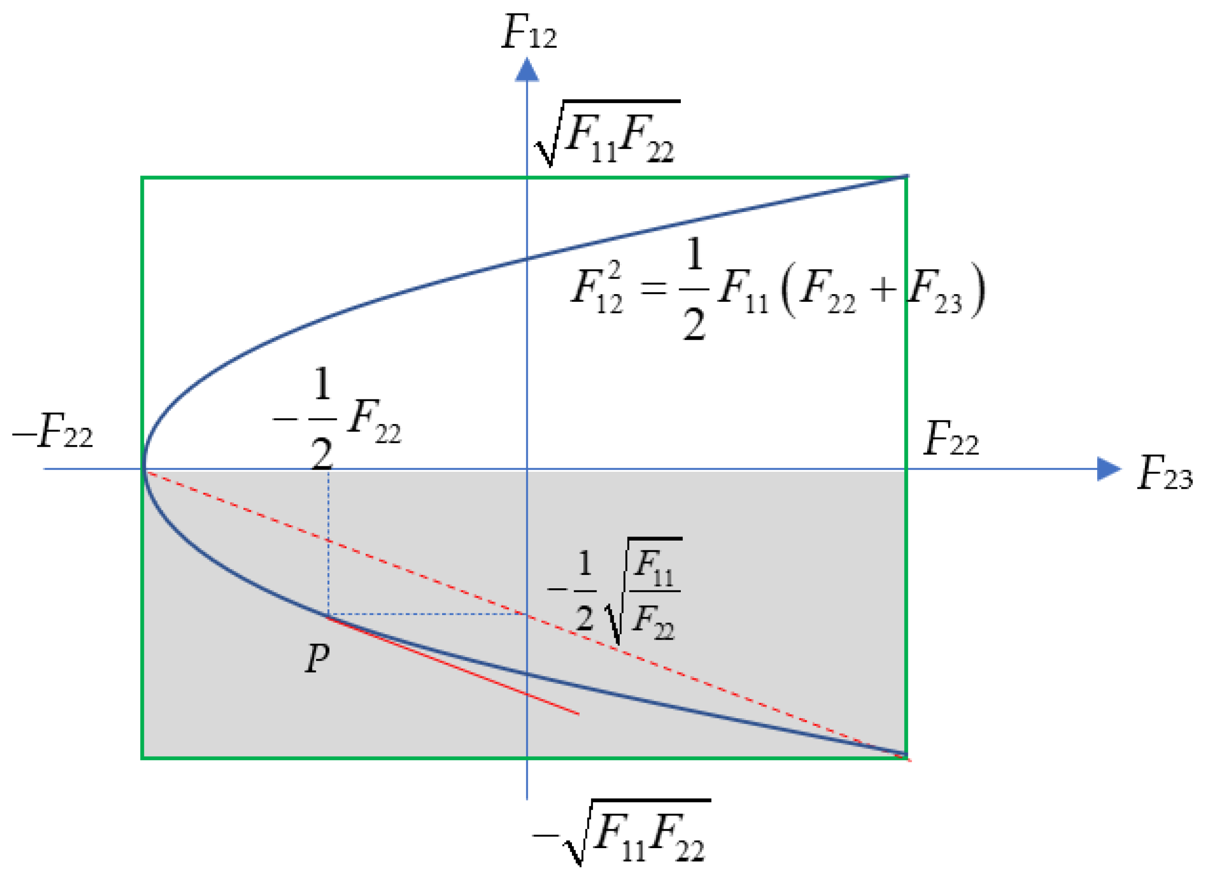
Equation (17) shows F12 as a function of F23, which is a parabola on the F23-F12 plane, as sketched in Figure 1. The domain of the function can be obtained from the first condition in (3). For transversely isotropic materials, it becomes:
In regard to the domain, the range of the function happens to coincide with the third condition in (3), i.e., , given that F11 and F22 are both positive and, hence, . The permissible values of F23 and F12 can only be within the green rectangle shown in Figure 1, with the parabola passing its two corners on the right and touching its side on the left.
Any point on the parabola in Figure 1 satisfies (17). To determine F12 and F23 completely means to fix a point on the parabola, referred to as point P. This requires one additional consideration that can be obtained by examining (17) in the context of its physical implications. The coefficients F12 and F23 are expressed one way or another in terms of strength properties, which are obtained experimentally; hence, errors are inevitable. Any perturbation due to an experimental error in one of the coefficients will have to be met by a variation in the other in order to keep (17) satisfied. If P is selected close to the tip of the parabola, where dF12/dF23 approaches infinity, it would require a large variation in F12 to correct a small perturbation in F23, making the failure criterion extremely sensitive to small errors in the evaluation of F23. Similarly, if P is placed close to the open end of the parabola, although the derivative is neither infinite nor zero, the failure criterion is bound to be more sensitive to F12 than to F23. Between these two extremes, according to the mean-value theorem [9], there exists an unbiased point where the failure criterion will be equally sensitive to the perturbations in F12 and F23. The question now is how to determine it logically.
The parabola shown in Figure 1 will be subject to further examination, as its intricacy has yet to be decoded. F12 as a function of F23 is apparently not single valued. The top and bottom halves of the parabola both provide a single valued branch. Following the relevant discussion in [6] on the sense of F12, for the quadratic form (11) to be an elliptic paraboloid with an opening on the triaxial compression side, the value of F12 must be negative; therefore, it is the lower half of the parabola in Figure 1 that should be considered as the permissible branch for p to fall upon. For this branch, the legitimate range of F12 is (0, ) as F23 varies within its range of (−F22, F22), covering the zone shaded in Figure 1. Both F12 and F23 can now be normalised with respect to the breadths of their single valued ranges as follows:
varies from 0 to –1 over a non-dimensional unit distance, while takes its value from −1/2 to 1/2, also covering a non-dimensional unit distance. Thus, both F12 and F23 are normalised in a consistent and unbiased manner. Accordingly, the expression of Δ as given in (15) can also be normalised as:
For to be equally sensitive to and in their unnormalized form, it is reasonable to expect that:
From (20), one obtains:
Thus, (21) leads to:
Since Δ = 0, its nondimensionalised form as defined in (20) should also vanish. Given (23), the relationship in (17) leads to:
Thus, both F12 and F23 are determined as shown above. Whilst the relationship in (17) represents a rigorous consideration from analytic geometry, the relationship in (21) results from the logical consideration of the unbiased sensitivity of the failure criterion to F12 and F23. The normalisations made to F12 and F23 in (19) ensure that they can be compared as like with like.
From (24), given the fourth condition of (9) and the expressions of F44 and F22 in (2), a natural consequence is:
This suggests that amongst the three transverse strengths—tensile, compressive and shear—of a transversely isotropic material, only two are independent as long as the failure criterion is based on a single quadratic function. Therefore, based on the elaboration presented above, the fully rationalised Tsai–Wu criterion can be delivered as follows:
where the coefficients are determined by conventional strength properties, as given in (2). It is clear that under triaxial compression at the following stress ratio:
whilst all shear stresses vanish, criterion (26) will never be satisfied, i.e., failure will never take place, implying an infinite strength under this special and unique stress state. In fact, the position holds even in presence of shear stresses. The triaxial compression at the ratio given in (27) has a reinforcing effect on the shear strengths. This can be seen clearly if (26) is re-written under this particular stress state as:
where σ is the magnitude of the transverse stresses (i.e., non-negative) of the triaxial compressive stress state.
For 2D stress states in the 1–2 plane, (26) is simplified to:
An important observation to make is that to predict the failure of a material under a 3D stress state from (26), the same set of strength properties is required as that for a 2D stress state from (29). It should be emphasised here that the rationalisation above has to be carried out on the criterion in its 3D form before it is reduced to 2D. Although (29) is a well-known form [11], its rational justification can be obtained only through the route of manipulating 3D stress states, as presented above.
4.3. Verification and Discussion
The point on the parabola given by (23) and (24) is special in multiple ways. It was argued above that it renders failure criterion (10) to be equally sensitive to F12 and F23 under the condition that the failure envelope is an elliptic paraboloid. The slope to the parabola at this point happens to be equal to the slope of the secant between the two extremes of the single valued branch concerned, i.e., the tip of the parabola and the bottom right end. The tangent and secant are marked in Figure 1 by solid and dashed red lines, respectively. Therefore, this is the point whose existence has been asserted by the mean-value theorem [9].
In order to interpret the results above and to verify the normalisations introduced in (19), all the terms in the failure criterion (10) are normalised as follows, which is similar to procedure used in [11].
where
The values of and as obtained in (23) and (24) are also incorporated above. All terms of the similar nature tend to contribute to F in the same way, whilst the differences due to the anisotropy of the material in all second order terms are absorbed in the normalisation scheme. The contributions of F12 and F23 obtained in (23) and (24) have indeed been equalised in their normalised form.
The outcomes presented in (23) and (24) rest heavily on the normalisations in (19). If one is prepared to accept (19) as the correct normalisations, which equalise the contributions of and to the failure function as the major premise for the deductive reasoning as presented above, conclusions (23) and (24) will be the logical consequence.
The existence of a relationship amongst transverse strengths, as shown in (24), can also be argued as follows. There are only two independent strength properties for isotropic materials of different tensile and compressive strengths for 3D stresses in general, as well as for any plane stress conditions as special cases, according to the established Raghava–Caddell–Yeh criterion [17], which has been more rationally formulated in [18]. When a transversely isotropic material is under a plane stress condition in its transverse plane, i.e., the 2–3 plane, the material is effectively isotropic; therefore, the Raghava–Caddell–Yeh criterion in its 2D form should be applicable. If so, it will only require two strength properties. For the Tsai–Wu criterion to reproduce the Raghava–Caddell–Yeh criterion under this condition, the third strength property cannot be independent.
With F12 and F23 as determined in (23) and (24), one can verify conditions in (16) as follows:
Hence, (11) defines an elliptic paraboloid. The inequality of (32) is met by most composites of practical importance and the only alternative is A = 0, which arises only under special conditions, as will be discussed later.
As a further verification, reducing the materials to isotropic materials of unequal tensile and compressive strengths, whilst (33) and (34) still hold:
In this case, Equation (10) leads to:
where and are the tensile and compressive strengths of the isotropic material, respectively. This reproduces the Raghava–Caddell–Yeh criterion [17], for which the failure envelope is a circular paraboloid demonstrating infinite strength against hydrostatic compression, but not hydrostatic tension.
As a case of further specialisation for isotropic materials of equal tensile and compressive strengths, i.e., , (36) further reduces to the von Mises criterion [13]:
where is the strength of the material, which the same for both tension and compression. This corresponds to the case when the condition for A > 0 does not hold. Given the expression of A in (32), the only alternative is A = 0. In this case, (10) turns into a cylindrical surface according to [9]. It can be seen that a cylindrical surface can be mathematically considered as an extreme case of an elliptic paraboloidal surface, allowing the von Mises criterion to be seen as a special case of the Tsai–Wu criterion.
As a further point of discussion, (24) shows that according to (8). Equation (7), as obtained in [6], naturally leads to (23), reproducing (6) as Tsai and Hahn suggested in [11]. However, the only justification given in [11] was that it allowed the Tsai–Wu criterion to reproduce the von Mises criterion for isotropic materials of equal tensile and compressive strengths, whereas in this paper, (23) and (24) were obtained simultaneously from systematic and logical deduction. In [6], it was suggested that δ was a material constant that could vary from between materials. Relationship (24) asserts further that δ is a universal constant, i.e., , for all transversely isotropic materials, brittle or ductile, including completely isotropic materials as a special case. This is apparently observed in isotropic materials obeying the Raghava–Caddell–Yeh criterion [17] and the von Mises criterion [13], as special cases. Any variation in δ, similar to those shown in [6], should be attributed to the variability of the experimentally measured transverse strength properties. This resembles a universal relationship amongst Young’s moduli and Poisson’s ratios, , although the underlying considerations are rather different. Raw experimental data would show significant variability as well if they were all independently measured.
4.4. Comparisons of Predicted Transverse Shear Strengths with Measured Values and Those from Other Theories
In the Puck failure criterion [14,15], the transverse shear strength is a derived quantity that is equal to the transverse tensile strength. In comparison to (25), it corresponds to the special case of . The transverse shear strengths obtained according to the Puck criterion and the present derivation are compared in Table 1 over a range of composites from [10,19,20] where experimental data are available. Relative to the measured values of in the third row of Table 1, those obtained from (25) outperform those from the Puck criterion, except for S-2 glass/Epoxy 2 and G40-800/5026, as highlighted in Table 1. For these two cases, one is only marginally worse than that predicted by the Puck criterion, whilst the other is identical to that predicted from the Puck criterion, because holds, although the experimental shear strength of 57 MPa is nearly 20% below for this particular material.
Given that is the strength of the material under pure transverse shear, as predicted from failure criterion (26), the degree of its agreement with the experimentally obtained transverse shear strength—i.e., the comparison between the measured values in the third row of Table 1—and that predicted from (25), as shown in the fourth rows of Table 1, can serve as a basic level of validation for the criterion (26). When applying (26) to problems involving general stress states, one should be prepared for discrepancies of a magnitude comparable with those between the figures in the third and fourth rows in Table 1, as an indication of the level of accuracy that criterion (26) is capable of offering.
Another relationship amongst transverse strengths can be found in [16], and is given as follows:
It is apparently a more complicated expression than that given in (25). The derivation in [16] was based on the following failure criterion stemming from Hashin’s matrix failure criterion [3] under a plane stress state in the transverse plane before it was split into tensile and compressive modes.
This is an incomplete quadratic form. The contributions from fibre direction as well as the interactive term associated with F12 have been excluded a priori.
The interaction between the stresses represented by F12 resembles the role of Poisson’s ratios in the generalised Hooke’s law in the theory of elasticity. It might be true that in the solutions to many elastic problems, the contributions from Poisson’s ratios are limited in terms of magnitude. Whilst ignoring such contributions would not lead to excessive error, the absence of Poisson’s ratios would prevent the appropriate understanding of many important mechanical behaviours of materials, such as the anticlastic behaviour, free edge effects, etc.
Similarly, to reveal the special relationships elaborated in this paper, it is important to incorporate the interactive terms in the failure criterion. The approach to treating the interactive terms can also be viewed as a meaningful indicator of the consistency of the formulation. For instance, in the well-known Hashin criterion [3], the interactive term F12 was ignored based on the assumption that failure is determined by stresses on the failure plane, which was inherited from the Mohr criterion [21] for isotropic materials; however, this particular assumption is inapplicable to anisotropic composites, as was argued in [22]. Whilst the numerical errors could be insignificant in many cases, as Hashin also stated in [3], the exclusion of such interactions would not allow the intricate relationships obtained in this paper to be revealed. From another perspective, including one interactive coefficient (F23) in the failure function, whilst excluding another (F12), as in [3], can at least be viewed as a degree of inconsistency. The numerical closeness of the results from a theory to experimental data in one aspect or another is important; however, we believe that the mathematical and logical consistency of the theory is even more important.
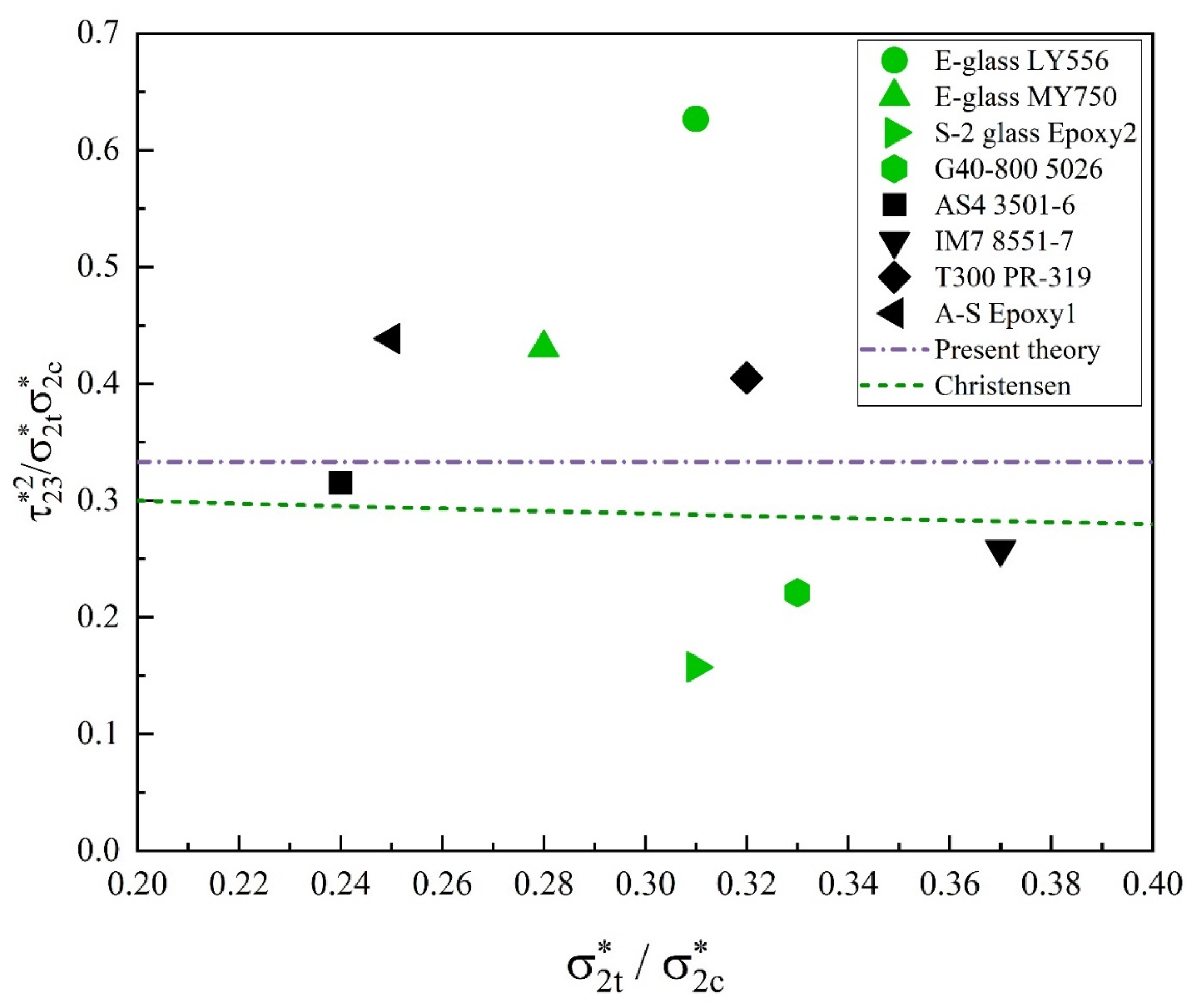
The numerical values obtained from (38) [16] over the same range of materials as above are also shown in the fifth row of Table 1. Relative to the experimental data in the third row of Table 1, the predictions from (25) listed in the fourth row of Table 1 outperform those from (38) for five out of eight materials. The trend is further shown graphically in Figure 2, where the ratio is plotted as a function of the ratio . The curve corresponding to (38) does not seem to be more representative than the straight line obtained according to (25), understanding the variability in measured transverse strengths as argued in [16]. The predictions are not more relevant to carbon composites (black symbols) than to glass composites (green symbols) either, as was claimed in [16].
Logically, the major premise underlying (38) is failure criterion (39), which is at its best a special form of the criterion based on the full quadratic failure function from which (26) is obtained. There is no reason to expect (39) to be more representative than (26). In [16], efforts were made to eliminate an independent strength property from (39) whilst keeping the manipulations all within the transverse plane.
5. Retrospection and Prospection
According to analytic geometry [9], the sufficient conditions for the failure envelope of transversely isotropic materials to be closed, i.e., to be an ellipsoidal surface, are:
where A, J and D are given in (12)–(14), respectively, and the following is another invariant of quadratic form (11):
Since I is always positive, given the expression of D in (14), and is always positive according to the fourth equation in (9) (because is always positive), conditions and can be re-written as:
With F12 as given in (23), if the transverse shear strength (and hence F44) was left as an independent property, (42) could not be satisfied in general. An ellipsoid could be guaranteed provided that was sufficiently large. In the case of isotropic materials obeying the von Mises criterion, as a special case of transversely isotropic materials, D = Δ = 0, which satisfies (24) or (25) under the condition of (23), but violates (42). In other words, (42) would prohibit (11) to degenerate to the von Mises criterion as a special case for isotropic materials of equal tensile and compressive strengths, because D = 0 as a necessary condition is shared by cylinders and elliptic paraboloids, but not by ellipsoids, according to analytic geometry. It is clear now that having a closed failure envelope and having the von Mises criterion as a special case are two mutually exclusive propositions. Sometimes, it only requires a very small experimental or data processing error to nudge D from positive to negative; then, the nature of the failure envelope would change dramatically from an ellipsoid to an elliptic paraboloid or a hyperboloid. Whilst the imposition of (17) alone eliminates the possibility of the failure envelope being an ellipsoid or hyperboloid, errors in measured transverse strengths could still make the elliptic paraboloid imaginary according to analytic geometry. Relationship (25), in addition to (23), not only ensures that the failure envelope is a real and unique elliptic paraboloid, but also offers a way to mitigate experimental errors amongst measured transverse strengths. This illustrates a perfect example of how mathematical consistency brings insight into physical problems.
The conventional Tsai–Wu criterion could degenerate to the von Mises criterion for isotropic materials of equal tensile and compressive strengths [11] because the failure envelope in the original Tsai–Wu criterion was not limited to an ellipsoid, no matter how much it was desired; it could be ellipsoid, elliptic paraboloid and different hyperboloids depending on the value of the transverse shear strength , whilst satisfying the inequalities in (3). The necessary conditions of (3) were far too loose to impose such a restriction. The controlling factor of the shape of the failure envelope rests on the transverse shear strength , which affects the values of various invariants, in particular D. Narrowing the failure envelope down to an elliptic paraboloid, as proposed in this paper, can help to filter out many physically prohibitive scenarios whilst restoring the mathematical and logical consistency of the Tsai–Wu criterion. This is the spirit of rationalisation.
The fully rationalised Tsai–Wu criterion for general 3D stress states is presented in (26). For this criterion, the transverse shear strength is not a required strength property, but it can be predicted from the criterion. There will inevitably be a discrepancy between the predicted value and the measured value. The available independently measured transverse shear strength should be used to correct the experimental errors in other transverse strength properties, instead of being employed as an independent strength property for the failure criterion based on a quadratic failure function. It should be employed to correct the transverse tensile and compressive strengths in order to minimise systematic errors in these measured strengths in the same way that the experimentally measured should be employed to correct , and , rather than being incorporated in the generalised Hooke’s law. A practical method of such corrections will be addressed in a subsequent publication.
The 2D version of the fully rationalised Tsai–Wu criterion is given in (29). Although it looks identical to its familiar form, as presented in [11], the transverse tensile and compressive strengths required to evaluate F22 should be understood as their corrected values using the transverse shear strength, whenever available. The rationalisation still makes a difference to the 2D Tsai–Wu criterion but in an implicit way.
The failure criterion for transversely isotropic materials based on a single quadratic failure function can now be considered fully established, with a complete understanding of the nature of a quadratic failure function having been achieved mathematically. It can be fully and logically defined with five independent strength properties, namely tensile and compressive strengths in the directions along fibres and transverse to fibres, and the in-plane shear strength. All coefficients involved in the failure function can be expressed with mathematical rigour and logical consistency. Any additional strength property employed as an independent one will compromise the consistency of the theoretical framework, even if they were experimentally measured.
Having established the failure criterion (26) as the fully rationalised Tsai–Wu criterion, any significant deficiency or genuine discrepancy with experimental observations can now be confidently attributed to the lack of representativeness of the basic assumptions underlying the criterion:
- (1)
- The transverse isotropy and homogeneity of the material;
- (2)
- Failure function being a single quadratic function.
Any deviation from these ideal positions will inevitably have an effect on the outcomes and should be anticipated in assessing the accuracy of the predictions. The use of these assumptions brings convenience but also restrictions. The obtained criterion can only be as accurate as its underlying assumptions allow. The consistent use of a quadratic function for a failure criterion helps to eliminate undue errors and anomalies due to mathematical and logical oversights, but not the generic deficiency due to these assumptions themselves.
The limitations of using a single quadratic function as the failure function could be improved whilst remaining within the framework of a phenomenological approach in one of two ways:
- (1)
- To use a higher order polynomial for the failure function;
- (2)
- To partition the stress space into subspaces and to use a quadratic function in each subspace.
Either way, the number of independent strength properties will inevitably increase. One should always bear in mind how the newly introduced properties are to be determined, experimentally or otherwise. Abandoning phenomenological approaches completely or discontinuing their improvement before alternatives are established is partially responsible for the confused state of the art on the subject of composite failure criteria. With consistency established, one would be in a position to explore meaningful ways of determining strength properties as required for alternatives to experimental measurements, for instance, molecular dynamics as investigated in [23], although the material used in [23] was not transversely isotropic.
The first option above seems to pose formidable difficulties, as the understanding of the analytic geometry of polynomial functions higher than the second order in multidimensional spaces has been very limited and is certainly far less than that of quadratic functions. This is not an attractive direction forward practically.
The second option is likely to offer a practical way forward. The Hashin criterion [3] can be seen as an attempt in this direction, followed by a wide range of different attempts, including those in [15,24]. However, it is the authors’ view that an appropriate rationalisation is necessary for the Hashin criterion before a fundamental breakthrough can be expected. This will be the objective of another one of our subsequent publications.
In the literature, there is lack of failure criteria for genuinely orthotropic materials, apart from the maximum stress/strain criteria. The Tsai–Wu criterion was nominally proposed for orthotropic materials. However, without the appropriate means to determine the coefficients to the interactive terms, it has never been applied seriously beyond transversely isotropic materials. This is a problem we will address in another subsequent publication.
6. Conclusions
Using a complete quadratic failure function, there is only one rational choice for the failure envelope—an elliptic paraboloid, as a single-sided open surface that allows infinite strength under a unique stress ratio in triaxial compression. Any alternative would lead to contradictions one way or another. This quadratic failure function can only accommodate five independent strength properties. Seven were initially introduced in the original Tsai–Wu criterion [1] after considerations of transverse isotropy. A relationship was established between the two interactive coefficients F12 and F23 based purely on analytic geometry. It ensures that the failure envelope is an elliptic paraboloid. A further relationship between these coefficients can be obtained from a logical consideration that the sensitivity of the failure criterion to these two coefficients should be unbiased. Thus, they can both be uniquely determined analytically as and . Although the former is well known, it can only be fully justified in presence of the latter, which can be re-written as , given the transverse isotropy of the material. This introduces a relationship amongst transverse strengths as a natural consequence of the rationalisation; the relationship is an intrinsic property of the quadratic failure function for transversely isotropic materials. Failing to comply with this relationship compromises the consistency of the criterion based on a single quadratic failure function.
Due to the high variability in the measured transverse strengths, the obtained relationship amongst transverse strengths may not be perfectly represented in the available experimental data. In presence of all three transverse strengths independently obtained experimentally, the transverse shear strength can be employed to validate the relationship in (25), i.e., . The failure criterion can only be as accurate as the agreement between and .
The fully rationalised Tsai–Wu criterion is given in (26) for 3D stress states. Its 2D version in (29) looks identical to its familiar form. Although no changes were made to (29), the rationalisation offers a firm basis for (29), and the determination of no longer relies on experimental data fitting or other empiricism, but on a rigorous deduction from the mathematical and logical consequences of the basic assumptions introduced instead.
The required five independent strength properties are limited to conventional and widely available tensile and compressive strengths in the directions along and transverse to fibres and the in-plane shear strength for the failure predictions of both 2D and 3D stress states.
The most significant outcome of the present paper is the achievement of a thorough understanding of the nature of the quadratic failure function, with its intrinsic relationships having been revealed. Obeying these relationships ensures the self-consistency of the failure criterion. This should conclude a phase of investigations on the subject of failure criteria involved in recent publications [6,16,25] based on a quadratic failure function, as far as transversely isotropic materials are concerned. The failure criterion given in (26) can be employed in design and analysis with confidence within its applicability defined by its assumptions, viz. the transverse isotropy and homogeneity of the material, and the failure function being a single quadratic function.
Author Contributions
Conceptualization, S.L.; methodology, S.L. and E.S.; validation, S.L., M.X. and E.S; formal analysis, S.L.; investigation, S.L.; writing—original draft preparation, S.L.; writing—S.L. and E.S.; visualization, S.L. All authors have read and agreed to the published version of the manuscript.
Funding
This research received no external funding.
Institutional Review Board Statement
Not applicable.
Informed Consent Statement
Not applicable.
Data Availability Statement
There is no additional data.
Acknowledgments
The second author wishes to acknowledge the financial support from CSC, China and the scholarship from the Faculty of Engineering, the University of Nottingham.
Conflicts of Interest
The authors declare no conflict of interest.
References
- Tsai, S.W.; Wu, E.M. A general theory of strength for anisotropic materials. J. Compos. Mater. 1971, 5, 58–80. [Google Scholar] [CrossRef]
- Gol’denblat, I.I.; Kopnov, V.A. Strength of glass-reinforced plastics in the complex stress state. Mekhanika Polim. 1965, 7, 70. [Google Scholar] [CrossRef]
- Hashin, Z. Failure criteria for unidirectional fiber composites. J. Appl. Mech. 1980, 47, 329–334. [Google Scholar] [CrossRef]
- Li, S.; Sitnikova, E. A critical review on the rationality of popular failure criteria for composites. Compos. Commun. 2018, 8, 7–13. [Google Scholar] [CrossRef]
- Li, S.; Sitnikova, E. Representative Volume Elements and Unit Cells—Concepts. Theory, Applications and Implementation; Woodhead Publishing Series in Composites Science and Engineering; Elsevier: Duxford, UK, 2019. [Google Scholar]
- Li, S.; Sitnikova, E.; Liang, Y.; Kaddour, A.-S. The Tsai-Wu failure criterion rationalised in the context of UD composites. Compos. Part A Appl. Sci. Manuf. 2017, 102, 207–217. [Google Scholar] [CrossRef]
- BS EN ISO 527; Plastics—Determination of Tensile Properties—Part 4: Test Conditions for Isotropic and Orthotropic Fibre-Reinforced Plastic Composites. The British Standards Institution: London, UK, 1997.
- ASTM D3039/D3039M-14; Standard Test Method for Tensile Properties of Polymer Matrix Composite Materials. ASTM International: West Conshohocken, PA, USA, 2014.
- Korn, G.A.; Korn, T.M. Mathematical Handbook for Scientists and Engineers; Sections 2.4, 3.5 & 4.7; McGraw-Hill: New York, NY, USA, 1968. [Google Scholar]
- Kaddour, A.S.; Hinton, M.J. Input data for test cases used in benchmarking triaxial failure theories of composites. J. Compos. Mater. 2012, 46, 2295–2312. [Google Scholar] [CrossRef]
- Tsai, S.W.; Hahn, H.T. Introduction to Composite Materials; Technomic Publishing Company: Westport, CT, USA, 1980. [Google Scholar]
- Clarkson, E. Hexcel 8552 AS4 Unidirectional Prepreg Qualification Statistical Analysis Report; FAA Special Project no SP4614WI-Q, Report No NCP-RP-2010-008 Rev D; Wichita State University: Wichita, KS, USA, 2011. [Google Scholar]
- Von Mises, R. Mechanik der Festen Körper im Plastisch-Deformablen Zustand; Nachrichten von der Gesellschaft der Wissenschaften zu Göttingen, Mathematisch-Physikalische Klasse; Gesellschaft der Wissenschaften zu Göttingen: Göttingen, Germany, 1913; pp. 582–592. [Google Scholar]
- Puck, A.; Schurmann, H. Failure analysis of FRP laminates by means of physically based phenomenological models. Compos. Sci. Tech. 1998, 58, 1045–1067. [Google Scholar] [CrossRef]
- Knops, M. Analysis of Failure in Fiber Polymer Laminates. The Theory of Alfred Puck; Springer: Berlin/Heidelberg, Germany, 2008. [Google Scholar]
- Christensen, R.M. Completion and closure on failure criteria for unidirectional fiber composite materials. ASME J. Appl. Mech. 2013, 81, 011011. [Google Scholar] [CrossRef]
- Raghava, R.; Caddell, R.M.; Yeh, G.S.Y. The macroscopic yield behaviour of polymers. J. Mater. Sci. 1973, 8, 225–232. [Google Scholar] [CrossRef] [Green Version]
- Christensen, R.M. The Theory of Materials Failure; Oxford University Press: Oxford, UK, 2013. [Google Scholar]
- Soden, P.D.; Hinton, M.J.; Kaddour, A.S. Lamina properties, lay-up configurations and loading conditions for a range of fibre-reinforced composite laminates. Compos. Sci. Technol. 1998, 58, 1011–1022. [Google Scholar] [CrossRef]
- Kaddour, A.S.; Hinton, M.J.; Smith, P.A.; Li, S. Mechanical properties and details of composite laminates for the test cases used in the third world-wide failure exercise. J. Compos. Mater. 2013, 47, 2427–2442. [Google Scholar] [CrossRef]
- Mohr, O. Welche Umstände bedingen die Elastizitätsgrenze und den Bruch eines Materials? Civilingenieur 1900, 44, 1572–1577. [Google Scholar]
- Li, S. A reflection on the Mohr failure criterion. Mech. Mater. 2020, 148, 103442. [Google Scholar] [CrossRef]
- Zho, Y.; Hu, M. Mechanical behaviors of nanocrystalline Cu/SiC composites: An atomistic investigation. Comput. Mater. Sci. 2017, 129, 129–136. [Google Scholar] [CrossRef] [Green Version]
- Pinho, S.T.; Dávila, C.G.; Iannucci, L.; Robinson, P. Failure Models and Criteria for FRP under in-Plane or Three-Dimensional Stress States including Shear Non-Linearity; NASA/TM-2005-213530; NASA Langley Research Center: Hampton, VA, USA, 2005. [Google Scholar]
- Christensen, R.M. Failure criteria for fiber composite materials, the astonishing sixty year search, definitive usable results. Compos. Sci. Tech. 2019, 182, 107718. [Google Scholar] [CrossRef]
Figure 1.
The relationship between F12 and F23 and their permissible ranges.

Figure 2.
Graph of versus .


Table 1.
Experimentally measured strengths and predicted transverse strengths according to different theories, all in MPa.
Table 1.
Experimentally measured strengths and predicted transverse strengths according to different theories, all in MPa.
| Category | Row No. | Strength | Type of Composite Considered | ||||||||
|---|---|---|---|---|---|---|---|---|---|---|---|
| AS4 3501-6 | T300 BSL914C | E-Glass LY556 | E-Glass MY750 | IM7 8551-7 | T300 PR-319 | A-SE poxy 1 | S-2 Glass Epoxy 2 | G40-800 5026 | |||
| Experimentally measured strengths | 1 | 48 | 27 | 35 | 40 | 68 | 40 | 38 | 56.5 | 70 | |
| 2 | 200 | 200 | 114 | 145 | 185 | 125 | 150 | 180 | 210 | ||
| 3 | 55 | N/A | 50 | 50 | 57 | 45 | 50 | 40 | 57 | ||
| 4 | Present from Equation (25). | 56.57 | 42.43 | 36.47 | 43.97 | 64.76 | 40.82 | 43.59 | 58.22 | 70.00 | |
| 5 | Puck [14,15], . | 48 | 27 | 35 | 40 | 68 | 40 | 38 | 56.5 | 70 | |
| 6 | Christenson, as shown in Equation (39) [16]. | 50.93 | 43.82 | 33.50 | 42.56 | 58.59 | 36.91 | 41.90 | 54.48 | 56.12 | |
Publisher’s Note: MDPI stays neutral with regard to jurisdictional claims in published maps and institutional affiliations. |
© 2022 by the authors. Licensee MDPI, Basel, Switzerland. This article is an open access article distributed under the terms and conditions of the Creative Commons Attribution (CC BY) license (https://creativecommons.org/licenses/by/4.0/).
Share and Cite
MDPI and ACS Style
Li, S.; Xu, M.; Sitnikova, E. The Formulation of the Quadratic Failure Criterion for Transversely Isotropic Materials: Mathematical and Logical Considerations. J. Compos. Sci. 2022, 6, 82. https://doi.org/10.3390/jcs6030082
AMA Style
Li S, Xu M, Sitnikova E. The Formulation of the Quadratic Failure Criterion for Transversely Isotropic Materials: Mathematical and Logical Considerations. Journal of Composites Science. 2022; 6(3):82. https://doi.org/10.3390/jcs6030082
Chicago/Turabian StyleLi, Shuguang, Mingming Xu, and Elena Sitnikova. 2022. "The Formulation of the Quadratic Failure Criterion for Transversely Isotropic Materials: Mathematical and Logical Considerations" Journal of Composites Science 6, no. 3: 82. https://doi.org/10.3390/jcs6030082